Strongly Local Hypergraph Diffusions for Clustering and Semi-supervised Learning

Abstract.

Hypergraph-based machine learning methods are now widely recognized as important for modeling and using higher-order and multiway relationships between data objects. Local hypergraph clustering and semi-supervised learning specifically involve finding a well-connected set of nodes near a given set of labeled vertices. Although many methods for local clustering exist for graphs, there are relatively few for localized clustering in hypergraphs. Moreover, those that exist often lack flexibility to model a general class of hypergraph cut functions or cannot scale to large problems. To tackle these issues, this paper proposes a new diffusion-based hypergraph clustering algorithm that solves a quadratic hypergraph cut based objective akin to a hypergraph analog of Andersen-Chung-Lang personalized PageRank clustering for graphs. We prove that, for graphs with fixed maximum hyperedge size, this method is strongly local, meaning that its runtime only depends on the size of the output instead of the size of the hypergraph and is highly scalable. Moreover, our method enables us to compute with a wide variety of cardinality-based hypergraph cut functions. We also prove that the clusters found by solving the new objective function satisfy a Cheeger-like quality guarantee. We demonstrate that on large real-world hypergraphs our new method finds better clusters and runs much faster than existing approaches. Specifically, it runs in a few seconds for hypergraphs with a few million hyperedges compared with minutes for a flow-based technique. We furthermore show that our framework is general enough that can also be used to solve other p-norm based cut objectives on hypergraphs.

1. Introduction

Two common scenarios in graph-based data analysis are: (i) What are the clusters, groups, modules, or communities in a graph? and (ii) Given some limited label information on the nodes of the graph, what can be inferred about missing labels? These statements correspond to the clustering and semi-supervised learning problems respectively, and while there exists a strong state of the art in algorithms for these problems on graphs (Zhou et al., 2003; Andersen et al., 2006; Gleich and Mahoney, 2015; Yang et al., 2020; Veldt et al., 2016, 2019; Joachims, 2003; Mahoney et al., 2012), research on these problems is currently highly active for hypergraphs (Yoshida, 2019; Li and Milenkovic, 2018; Veldt et al., 2020b; Ibrahim and Gleich, 2020; Yin et al., 2017; Chitra and Raphael, 2019; Zhang et al., 2017) building on new types of results (Hein et al., 2013; Li and Milenkovic, 2017; Veldt et al., 2020a) compared to prior approaches (Karypis et al., 1999; Zhou et al., 2006; Agarwal et al., 2006). The lack of flexible, diverse, and scalable hypergraph algorithms for these problems limits the opportunities to investigate rich structure in data. For example, clusters can be relevant treatment groups for statistical testing on networks (Eckles et al., 2017) or identify common structure across many types of sparse networks (Leskovec et al., 2009). Likewise, semi-supervised learning helps to characterize subtle structure in the emissions spectra of galaxies in astronomy data through characterizations in terms of biased eigenvectors (Lawlor et al., 2016). The current set of hypergraph algorithms are insufficient for such advanced scenarios.

Hypergraphs, indeed, enable a flexible and rich data model that has the potential to capture subtle insights that are difficult or impossible to find with traditional graph-based analysis (Benson et al., 2016; Yin et al., 2017; Li and Milenkovic, 2018; Veldt et al., 2020b; Yoshida, 2019). But, hypergraph generalizations of graph-based algorithms often struggle with scalability and interpretation (Agarwal et al., 2006; Hein et al., 2013) with ongoing questions of whether particular models capture the higher-order information in hypergraphs. Regarding scalablility, an important special case for that is a strongly local algorithm. Strongly local algorithms are those whose runtime depends on the size of the output rather than the size of the graph. This was only recently addressed for various hypergraph clustering and semi-supervised learning frameworks (Veldt et al., 2020b; Ibrahim and Gleich, 2020). This property enables fast (seconds to minutes) evaluation even for massive graphs with hundreds of millions of nodes and edges (Andersen et al., 2006) (compared with hours). For graphs, perhaps the best known strongly local algorithm is the Andersen-Chung-Lang (henceforth, ACL) approximation for personalized PageRank (Andersen et al., 2006) with applications to local community detection and semi-supervised learning (Zhou et al., 2003). The specific problem we address is a mincut-inspired hypergraph generalization of personalized PageRank along with a strongly local algorithm to rapidly approximate solutions. Our formulation differs in a number of important ways from existing Laplacian (Zhou et al., 2006) and quadratic function-based hypergraph PageRank generalizations (Li and Milenkovic, 2018; Li et al., 2020; Takai et al., 2020).

Although our localized hypergraph PageRank is reasonably simple to state formally (§3.2), there are a variety of subtle aspects to both the problem statement and the algorithmic solution. First, we wish to have a formulation that enables the richness of possible hypergraph cut functions. These hypergraph cut functions are an essential component to rich hypergraph models because they determine when a group of nodes ought to belong to the same cluster or obtain a potential new label for semi-supervised learning. Existing techniques based on star expansions (akin to treating the hypergraph as a bipartite graph) or a clique expansion (creating a weighted graph by adding edges from a clique to the graph for each hyperedge) only model a limited set of cut functions (Agarwal et al., 2005; Veldt et al., 2020a). More general techniques based on Lovász extensions (Li and Milenkovic, 2018; Li et al., 2020; Yoshida, 2019) pose substantial computational difficulties. Second, we need a problem framework that gives sparse solutions such that they can be computed in a strongly local fashion and then we need an algorithm that is actually able to compute these—the mere existence of solutions is insufficient for deploying these ideas in practice as we wish to do. Finally, we need an understanding of the relationship between the results of this algorithm and various graph quantities, such as minimal conductance sets as in the original ACL method.

To address these challenges, we extend and employ a number of recently proposed hypergraph frameworks. First, we show a new result on a class of hypergraph to graph transformations (Veldt et al., 2020a). These transformations employ carefully constructed directed graph gadgets, along with a set of auxiliary nodes, to encode the properties of a general class of cardinality based hypergraph cut functions. Our simple new result highlights how these transformations not only preserve cut values, but preserve the hypergraph conductance values as well (§3.1). Then we localize the computation in the reduced graph using a general strategy to build strongly local computations. This involves a particular modification often called a “localized cut” graph or hypergraph (Liu and Gleich, 2020; Veldt et al., 2020b; Andersen and Lang, 2008; Fountoulakis et al., 2020). We then use a squared $2$-norm (i.e. a quadratic function) instead of a $1$-norm that arises in the mincut-graph to produce the hypergraph analogue to strongly local personalized PageRank. Put another way, applying all of these steps on a graph (instead of a hypergraph) is equivalent to a characterization of personalized PageRank vector (Gleich and Mahoney, 2014).

Once we have the framework in place (§3.1,§3.2), we are able to show that an adaptation of the push method for personalized PageRank (§3.3) will compute an approximate solution in time that depends only on the localization parameters and is independent of the size of a hypergraph with fixed maximum hyperedge size (Theorem 3.5). Consequently, the algorithms are strongly local.

The final algorithm we produce is extremely efficient. It is a small factor (2-5x) slower than running the ACL algorithm for graphs on the star expansion of the hypergraph. It is also a small factor (2-5x) faster than running an optimized implementation of the ACL algorithm on the clique expansion of the hypergraph. Nevertheless, for many instances of semi-supervised learning problems, it produces results with much larger F1 scores than alternative methods. In particular, it is much faster and performs much better with extremely limited label information than a recently proposed flow-based method (Veldt et al., 2020b).

Summary of additional contributions. In addition to providing a strongly local algorithm for the squared $2$-norm (i.e. a quadratic function) in §3.2, which gives better and faster empirical performance (§7), we also discuss how to use a $p$-norm (§6) instead. Finally, we also show a Cheeger inequality that relates our results to the hypergraph conductance of a nearby set (§4).

Our method is the first algorithm for hypergraph clustering that includes all of the following features: it is (1) strongly-local, (2) can grow a cluster from a small seed set, (3) models flexible hyperedge cut penalties, and (4) comes with a conductance guarantee.

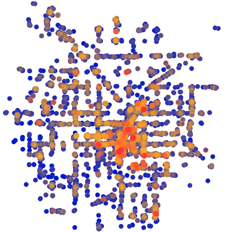
ACL-Clique
P=0.80, R=0.99, F1=0.876

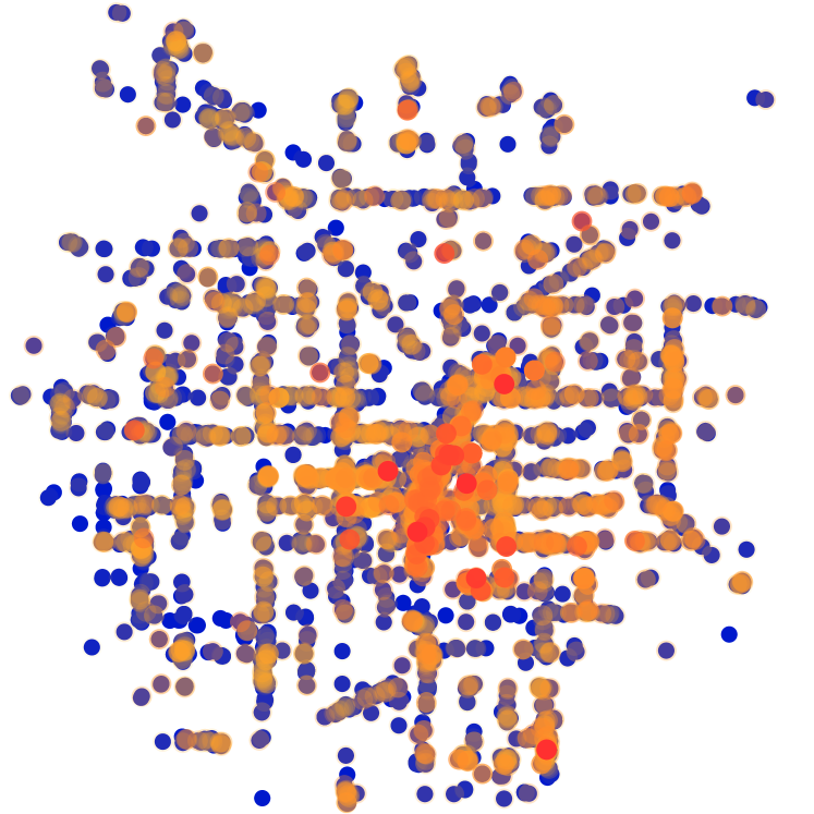
ACL-Star
P=0.76, R=0.98, F1=0.85

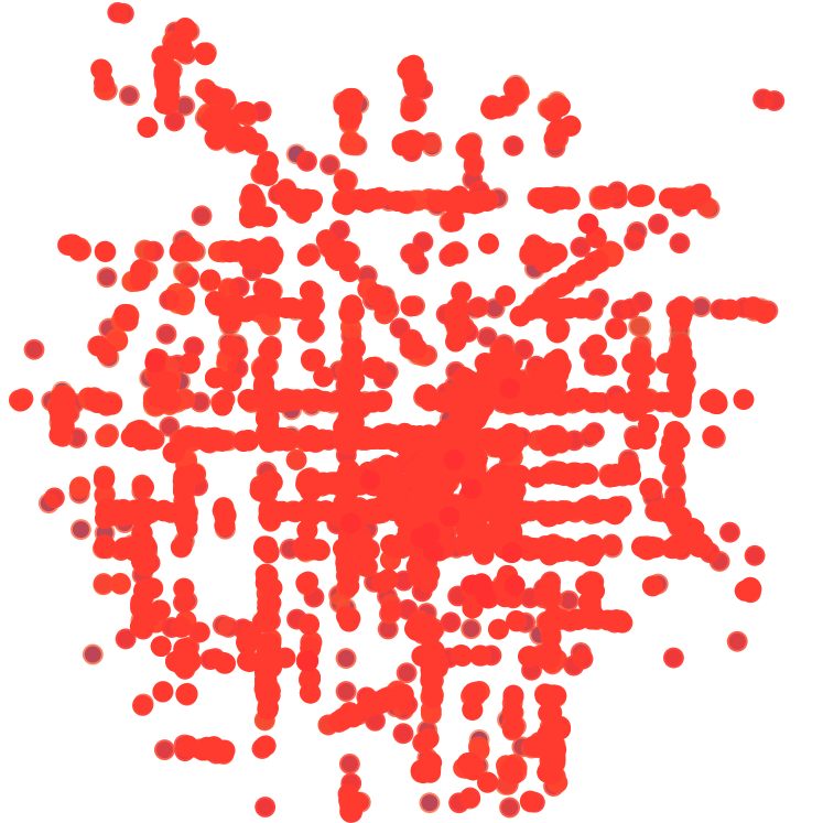
HyperLocal (Veldt et al., 2020b)
P=0.92, R=0.05, F1=0.10

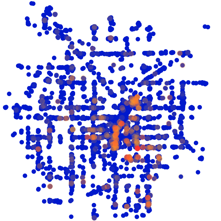
QHPR (Takai et al., 2020; Li et al., 2020)
P=0.83, R=0.95, F1=0.886

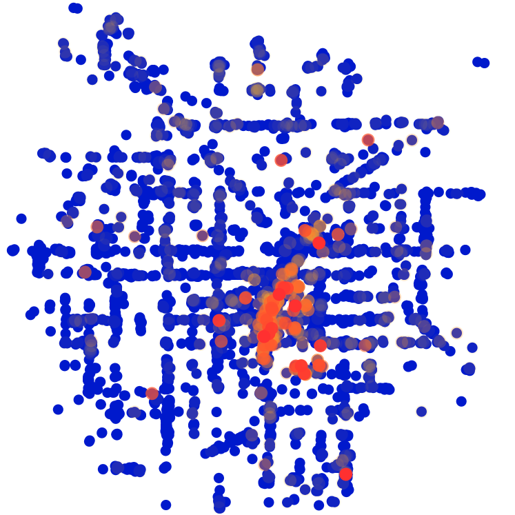
LHPR (Ours)
P=0.83, R=0.98, F1=0.900

Figure 1. This figure shows locations of the $\sim$7,300 restaurants of Las Vegas that are reviewed on Yelp and how often algorithms recover them from a set of 10 random seeds; our hypergraph PageRank (LHPR) methods has the highest accuracy and finds the result by exploring only 10000 vertices total compared with a fully dense vector for QHPR giving a boost to scalability on larger graphs. The colors show the regions that are missed (red or orange) or found (blue) by each algorithm over 15 trials. HyperLocal is a flow-based method that is known to have trouble growing small seed sets as in this experiment. (The parameters for HyperLocal were chosen in consultation its authors; other parameters were hand tuned for best case performance.)

A motivating case study with Yelp reviews. We begin by illustrating the need and utility for the methods instead with a simple example of the benefit to these spectral or PageRank-style hypergraph approaches. For this purpose we consider a hypothetical use case with an answer that is easy to understand in order to compare our algorithm to a variety of other approaches. We build a hypergraph from the Yelp review dataset (https://www.yelp.com/dataset). Each restaurant is a vertex and each user is a hyperedge. This model enables users, i.e. hyperedges, to capture subtle socioeconomic status information as well as culinary preferences in terms of which types of restaurants they visit and review. The task we seek to understand is either an instance of local clustering or semi-supervised learning. Simply put, given a random sample of 10 restaurants in Las Vegas Nevada, we seek to find other restaurants in Las Vegas. The overall hypergraph has around 64k vertices and 616k hyperedges with a maximum hyperedge size of 2566. Las Vegas, with around 7.3k restaurants, constitutes a small localized cluster.

We investigate a series of different algorithms that will identify a cluster nearby a seed node in a hypergraph: (1) Andersen-Chung-Lang PageRank on the star and clique expansion of the hypergraph (ACL-Star, ACL-Clique, respectively), these algorithms are closely related to ideas proposed in (Zhou et al., 2006; Agarwal et al., 2006); (2) HyperLocal, a recent maximum flow-based hypergraph clustering algorithm (Veldt et al., 2020b); (3) quadratic hypergraph PageRank (Li et al., 2020; Takai et al., 2020) (which is also closely related to (Hein et al., 2013)), and (4) our Local Hypergraph-PageRank (LHPR). These are all strongly local except for (3), which we include because our algorithm LHPR is essentially the strongly local analogue of (3).

The results are shown in Figure 1. The flow-based HyperLocal method has difficulty finding the entire cluster. Flow-based methods are known to have trouble expanding small seed sets (Veldt et al., 2016; Fountoulakis et al., 2020; Liu and Gleich, 2020) and this experiment shows that same behavior. Our strongly local hypergraph PageRank (LHPR) slightly improves on the performance of a quadratic hypergraph PageRank (QHPR) that is not strongly local. In particular, it has 10k non-zero entries (of 64k) in its solution.

This experiment shows the opportunities with our approach for large hypergraphs. We are able to model a flexible family of hypergraph cut functions beyond those that use clique and star expansions and we equal or outperform all the other methods. For instance, another more complicated method (Ibrahim and Gleich, 2020) designed for small hyperedge sizes showed similar performance to ACL-Clique (F1 around 0.85) and took much longer.

2. Notation and Preliminaries

Let $G=(V,E,w)$ be a directed graph with $|V|=n$ and $|E|=m$. For simplicity, we require weights $w_{ij}\geq 1$ for each directed edge $(i,j)\in E$. We interpret an undirected graph as having two directed edges $(i,j)$ and $(j,i)$. For simplicity, we assume the vertices are labeled with indices $1$ to $n$, so that we may use these labels to index matrices and vectors. For instance, we define $\boldsymbol{\mathrm{d}}$ as the length-$n$ out-degree vector where its $i$th component $d_{i}=\sum_{j\in V}w_{ij}$. The incidence matrix $\boldsymbol{\mathrm{B}}\in\{0,-1,1\}^{m\times n}$ measures the difference of adjacent nodes. The $k$th row of $\boldsymbol{\mathrm{B}}$ corresponds to an edge, say $(i,j)$, and has exactly two nonzero values, 1 for the node $i$ and -1 for the node $j$. (Recall that we have directed edges, so the origin of the edge is always $1$ and the destination is always -1.)

Let $\mathcal{H}=(V,\mathcal{E})$ be a hypergraph where each hyperedge $e\in\mathcal{E}$ is a subset of $V$. Let $\zeta=\max_{e\in\mathcal{E}}|e|$ be the maximum hyperedge size. With each hyperedge, we associate a splitting function $f_{e}$ that we use to assess an appropriate penalty for splitting the hyperedge among two labels or splitting the hyperedge between two clusters. Formally, let $S$ be a cluster and let $A=e\cap S$ be the hyperedge’s nodes inside $S$, then $f_{e}(A)$ penalizes splitting $e$. A common choice in early hypergraph literature was the all-or-nothing split, which assigns a fixed value if a hyperedge is split or zero if all nodes in the hyperedge lie in the same cluster (Hadley, 1995; Ihler et al., 1993; Lawler, 1973): $f_{e}(A)=0$ if $A=e$ or $A=\emptyset$ and $f_{e}(A)=1$ otherwise (or an alternative constant). More recently, there have been a variety of alternative splitting functions proposed (Li and Milenkovic, 2018, 2017; Veldt et al., 2020a) that provide more flexibility. We discuss more choices in the next section (§3.1). With a splitting function identified, the cut value of any given set $S$ can be written as $\text{cut}_{\mathcal{H}}(S)=\sum_{e\in E}f_{e}(e\cap S)$. The node degree in this case can be defined as $d_{i}=\sum_{e:i\in e}f_{e}(\{i\})$ (Li and Milenkovic, 2017; Veldt et al., 2020b), though other types of degree vectors can also be used in both the graph and hypergraph case. This gives rise to a definition of conductance on a hypergraph

(1) $$\phi_{\mathcal{H}}(S)=\frac{\textbf{cut}_{\mathcal{H}}(S)}{\text{min}(\textbf{vol}(S),\textbf{vol}(\bar{S}))}$$

where $\textbf{vol}(S)=\sum_{i\in S}d_{i}$. This reduces to the standard definition of graph conductance when each edge has only two nodes ($\zeta=2$) and we use the all-or-nothing penality.

Diffusion algorithms for semi-supervised learning and local clustering. Given a set of seeds, or what we commonly think of as a reference, set $R$, a diffusion is any method that produces a real-valued vector $\boldsymbol{\mathrm{x}}$ over all the other vertices. For instance, the personalized PageRank method uses $R$ to define the personalization vector or restart vector underlying the process (Andersen et al., 2006). The PageRank solution or the sparse Andersen-Chung-Lang approximation (Andersen et al., 2006) are then the diffusion $\boldsymbol{\mathrm{x}}$. Given a diffusion vector $\boldsymbol{\mathrm{x}}$, we round it back to a set $S$ by performing a procedure called a sweepcut. This involves sorting $\boldsymbol{\mathrm{x}}$ from largest to smallest and then evaluating the hypergraph conductance of each prefix set $S_{j}=\{[1],[2],\ldots,[k]\}$, where $[i]$ is the id of the $i$th largest vertex. The set returned by sweepcut picks the minimum conductance set $S_{j}$. Since the sweepcut procedures are general and standardized, we focus on the computation of $\boldsymbol{\mathrm{x}}$. When these algorithms are used for semi-supervised learning, the returned set $S$ is presumed to share the label as the reference (seed) set $R$; alternatively, its value or rank information may be used to disambiguate multiple labels (Zhou et al., 2003; Gleich and Mahoney, 2015).

3. Method

Our overall goal is to compute a hypergraph diffusion that will help us perform a sweepcut to identify a set with reasonably small conductance nearby a reference set of vertices in the graph. We explain our method: localized hypergraph quadratic diffusions (LHQD) or also localized hypergraph PageRank (LHPR) through two transformations before we formally state the problem and algorithm. We adopted this strategy so that the final proposal is well justified because some of the transformations require additional context to appreciate. Computing the final sweepcut is straightforward for hypergraph conductance, and so we do not focus on that step.

3.1. Hypergraph-to-graph reductions

Minimizing conductance is NP-hard even in the case of simple graphs, though numerous techniques have been designed to approximate the objective in theory and practice (Andersen and Lang, 2008; Andersen et al., 2006; Chung, 1992). A common strategy for searching for low-conductance sets in hypergraphs is to first reduce a hypergraph to a graph, and then apply existing graph-based techniques. This sounds “hacky” or least “ad-hoc” but this idea is both principled and rigorous. The most common approach is to apply a clique expansion (Benson et al., 2016; Li and Milenkovic, 2017; Zien et al., 1999; Zhou et al., 2006; Agarwal et al., 2006), which explicitly models splitting functions of the form $f_{e}(A)\propto|A||e\backslash A|$. For instance Benson et al. (Benson et al., 2016) showed that clique expansion can be used to convert a 3-uniform hypergraph into a graph that preserves the all-or-nothing conductance values. For larger hyperedge sizes, all-or-nothing conductance is preserved to within a distortion factor depending on the size of the hyperedge. Later, Li et al. (Li and Milenkovic, 2017) were the first to introduce more generalized notions of hyperedge splitting functions, focusing specifically on submodular functions.

Definition 3.1.

A splitting function $f_{e}$ is submodular if

(2) $$f_{e}(A)+f_{e}(B)\geq f_{e}(A\cup B)+f_{e}(A\cap B)\quad\text{$\forall A,B\subseteq e$}.$$

These authors showed that for this submodular case, clique expansion could be used to define a graph preserving conductance to within a factor $O(\zeta)$ ($\zeta$ is the largest hyperedge size).

More recently, Veldt et al. (Veldt et al., 2020a) introduced graph reduction techniques that exactly preserve submodular hypergraph cut functions which are cardinality-based.

Definition 3.2.

A splitting function $f_{e}$ is cardinality-based if

(3) $$f_{e}(A)=f_{e}(B)\quad\text{whenever $|A|=|B|$}.$$

Cardinality-based splitting functions are a natural choice for many applications, since node identification is typically irrelevant in practice, and the cardinality-based model produces a cut function that is invariant to node permutation. Furthermore, most previous research on applying generalized hypergraph cut penalties implicitly focused on cut functions are that are naturally cardinality-based (Li and Milenkovic, 2018; Li et al., 2020; Hein et al., 2013; Benson et al., 2016; Zien et al., 1999; Karypis et al., 1999). Because of their ubiquity and flexibility, in this work we also focus on hypergraph cut functions that are submodular and cardinality-based. We briefly review the associated graph transformation and then we build on previous work by showing that these hypergraph reductions can be used to preserve the hypergraph conductance objective, and not just hypergraph cuts.

Reduction for Cardinality-Based Cuts. Veldt et al. (Veldt et al., 2020a) gave results that show the cut properties of a submodular, cardinality-based hypergraph could be preserved by replacing each hyperedge with a set of directed graph gadgets. Each gadget for a hyperedge $e$ is constructed by introducing a pair of auxiliary nodes $a$ and $b$, along with a directed edge $(a,b)$ with weight $\delta_{e}>0$. For each $v\in e$, two unit-weight directed edges are introduced: $(v,a)$ and $(b,v)$. The entire gadget is then scaled by a weight $c_{e}\geq 0$. The resulting gadget represents a simplified splitting function of the following form:

(4) $$f_{e}(A)=c_{e}\cdot\min\{|A|,|e\backslash A|,\delta_{e}\}.$$

Figure 2(b) illustrates the process of replacing a hyperedge with a gadget. The cut properties of any submodular cardinality-based splitting function can be exactly modeled by introducing a set of $O(|e|)$ or fewer such splitting functions (Veldt et al., 2020a). If an approximation suffices, only $O(\log|e|)$ gadgets are required (Benson et al., 2020).

(a) original hypergraph

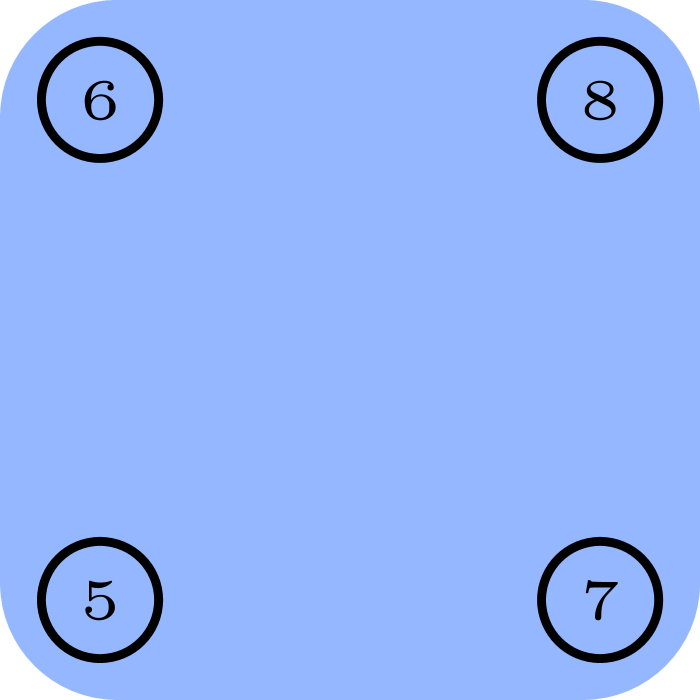
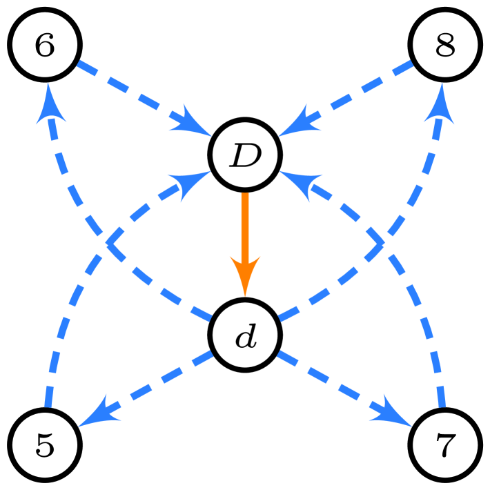
(b) single hyperedge reduction gadget

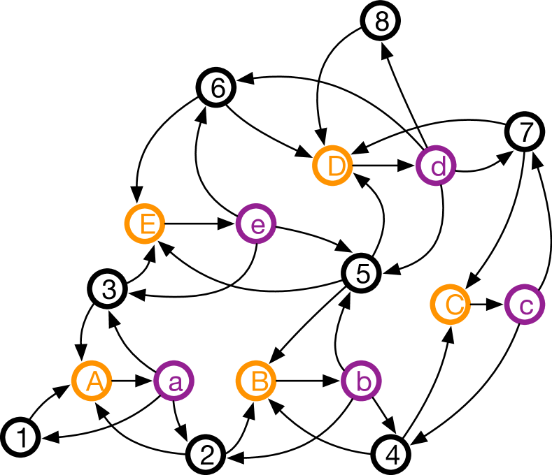
(c) expanded graph

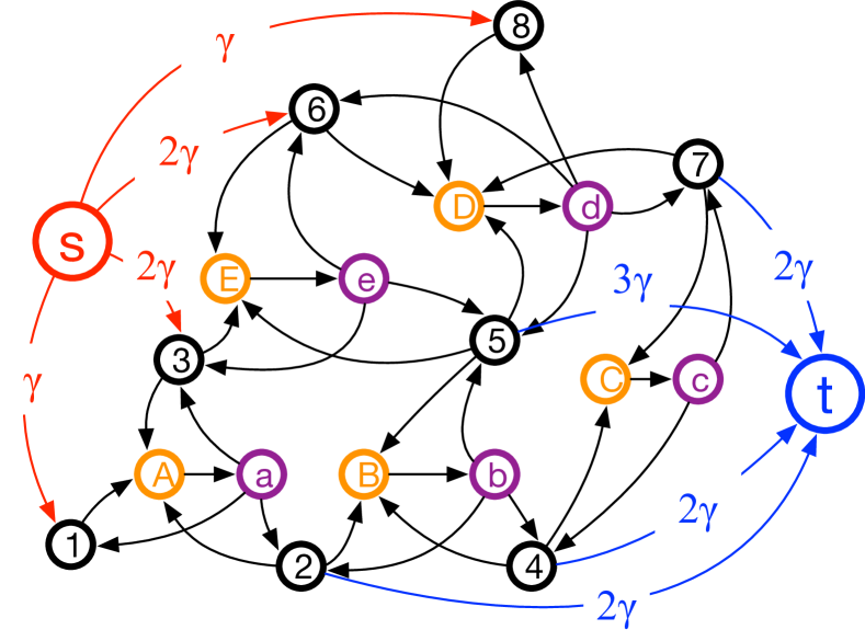
(d) localized directed cut graph

Figure 2. A simple illustration of hypergraph reduction (Section 3.1) and localization (Section 3.2). (a) A hypergraph with 8 nodes and 5 hyperedges. (b) An illustration of the hyperedge transformation gadget for $\delta$-linear splitting function. (c) The hypergraph is reduced to a directed graph by adding a pair of auxiliary nodes for each hyperedge and this preserves hypergraph conductance computations (Theorem 3.3). (d) The localized directed cut graph is created by adding a source node $s$, a sink node $t$ and edges from $s$ to hypergraph nodes or from hypergraph nodes to $t$ to localize a solution.

An important consequence of these reduction results is that in order to develop reduction techniques for any submodular cardinality-based splitting functions, it suffices to consider hyperedges with splitting functions of the simplified form given in (4). In the remainder of the text, we focus on splitting functions of this form, with the understanding that all other cardinality-based submodular splitting functions can be modeled by introducing multiple hyperedges on the same set of nodes with different edge weights.

In Figure 2, we illustrate the procedure of reducing a small hypergraph to a directed graph, where we introduce a single gadget per hyperedge. Formally, for a hypergraph $\mathcal{H}=(V,E)$, this procedure produces a directed graph $G=(\hat{V},\hat{E})$, with directed edge set $\hat{E}$, and node set $\hat{V}=V\cup V_{a}\cup V_{b}$, where $V$ is the set of original hypergraph nodes. Sets $V_{a},V_{b}$ store auxiliary nodes, in such a way that for each pair of auxiliary nodes $a,b$ where $(a,b)$ is a directed edge, we have $a\in V_{a}$ and $b\in V_{b}$. This reduction technique was previously developed as a way of preserving minimum cuts and minimum $s$-$t$ cuts for the original hypergraph. Here, we extend this result to show that for a certain choice for node degree, this reduction also preserves hypergraph conductance.

Theorem 3.3.

Define a degree vector $\boldsymbol{\mathrm{d}}$ for the reduced graph $G=(\hat{V},\hat{E})$ such that $\boldsymbol{\mathrm{d}}(v)=d_{v}$ is the out-degree for each node $v\in V$, and $\boldsymbol{\mathrm{d}}(u)=d_{u}=0$ for every auxiliary node $u\in V_{a}\cup V_{b}$. If $T^{*}$ is the minimum conductance set in $G$ for this degree vector, then $S^{*}=T^{*}\cap V$ is the minimum hypergraph conductance set in $\mathcal{H}=(V,E)$.

Proof.

From previous work on these reduction techniques (Benson et al., 2020; Veldt et al., 2020a), we know that the cut penalty for a set $S\subseteq V$ in $\mathcal{H}$ equals the cut penalty in the directed graph, as long as auxiliary nodes are arranged in a way that produces the smallest cut penalty subject to the choice of node set $S\subseteq V$. Formally, for $S\subseteq V$,

(5) $$\textbf{cut}_{\mathcal{H}}(S)=\operatorname*{minimize}_{T\subset\hat{V}\colon S=T\cap V}\textbf{cut}_{G}(T),$$

where $\textbf{cut}_{G}$ denotes the weight of directed out-edges originating inside $S$ that are cut in $G$. By our choice of degree vector, the volume of nodes in $G$ equals the volume of the non-auxiliary nodes in $\mathcal{H}$. That is, for all $T\subseteq\hat{V}$, $\textbf{vol}_{G}(T)=\sum_{v\in V}d_{v}+\sum_{u\in V_{a}\cup V_{b}}d_{u}=\textbf{vol}_{G}(T\cap V)=\textbf{vol}_{\mathcal{H}}(T\cap V)$. Let $T^{*}\subseteq\hat{V}$ be the minimum conductance set in $G$, and $S^{*}=T^{*}\cap V$. Without loss of generality we can assume that $\textbf{vol}_{G}(T^{*})\leq\textbf{vol}_{G}(\bar{T}^{*})$. Since $T^{*}$ minimizes conductance, and auxiliary nodes have no effect on the volume of this set, $\textbf{cut}_{G}(T^{*})=\operatorname*{minimize}_{T\subset\hat{V}\colon T\cap S^{*}}\textbf{cut}_{G}(T)=\textbf{cut}_{\mathcal{H}}(S^{*})$, and so ${\textbf{cut}_{G}(T^{*})}/{\textbf{vol}_{G}(T^{*})}={\textbf{cut}_{\mathcal{H}}(S^{*})}/{\textbf{vol}_{\mathcal{H}}(S^{*})}$. Thus, minimizing conductance in $G$ minimizes conductance in $\mathcal{H}$. ∎

3.2. Localized Quadratic Hypergraph Diffusions

Having established a conductance-preserving reduction from a hypergraph to a directed graph, we now present a framework for detecting localized clusters in the reduced graph $G$. To accomplish this, we first define a localized directed cut graph, involving a source and sink nodes and new weighted edges. This approach is closely related to previously defined localized cut graphs for local graph clustering and semi-supervised learning (Andersen and Lang, 2008; Gleich and Mahoney, 2014; Veldt et al., 2016; Liu and Gleich, 2020; Zhu et al., 2003; Blum and Chawla, 2001), and a similar localized cut hypergraph used for flow-based hypergraph clustering (Veldt et al., 2020b). The key conceptual difference is that we apply this construction directly to the reduced graph $G$, which by Theorem 3.3 preserves conductance of the original hypergraph $\mathcal{H}$. Formally, we assume we are given a set of nodes $R\subseteq V$ around which we wish to find low-conductance clusters, and a parameter $\gamma>0$. The localized directed cut graph is defined by applying the following steps to $G$:

• Introduce a source node $s$, and for each $r\in R$ define a directed edge $(s,r)$ of weight $\gamma d_{r}$

• Introduce a sink node $t$, and for each $v\in\bar{R}$ define a directed edge $(v,t)$ with weight $\gamma d_{v}$.

We do not connect auxiliary nodes to the source or sink, which is consistent with the fact that their degree is defined to be zero in order for Theorem 3.3 to hold. We illustrate the construction of the localized directed cut graph in Figure 2(d). It is important to note that in practice we do not in fact form this graph and store it in memory. Rather, this provides a conceptual framework for finding localized low-conductance sets in $G$, which in turn correspond to good clusters in $\mathcal{H}$.

Definition: Local hypergraph quadratic diffusions. Let $\boldsymbol{\mathrm{B}}$ and $\boldsymbol{\mathrm{w}}$ be the incidence matrix and edge weight vector of the localized directed cut graph with $\gamma$. The objective function for our hypergraph clustering diffusion, which we call local hypergraph quadratic diffusion or simply local hypergraph PageRank, is

(6) $$\begin{array}[]{ll}\displaystyle\operatorname*{minimize}_{\boldsymbol{\mathrm{x}}}&{\frac{1}{2}\boldsymbol{\mathrm{w}}^{T}(\boldsymbol{\mathrm{B}}\boldsymbol{\mathrm{x}})^{2}_{+}+\kappa\gamma\sum_{i\in V}x_{i}d_{i}}\\ \text{subject to}&{x_{s}=1,x_{t}=0,\boldsymbol{\mathrm{x}}\geq 0.}\end{array}$$

We use the function $(x)_{+}=\max\{x,0\}$, applied element-wise to $\boldsymbol{\mathrm{B}}\boldsymbol{\mathrm{x}}$, to indicate we only keep the positive elements of this product. This is analogous to the fact that we only view a directed edge as being cut if it crosses from the source to the sink side; this is similar to previous directed cut minorants on graphs and hypergraphs (Yoshida, 2016). The first term in the objective corresponds to a 2-norm minorant of the minimum $s$-$t$ cut objective on the localized directed cut graph. (In an undirected regular graph, the term $\boldsymbol{\mathrm{w}}^{T}(\boldsymbol{\mathrm{B}}\boldsymbol{\mathrm{x}})_{+}$ turns into an expression with the Laplacian, which can in turn be formally related to PageRank (Gleich and Mahoney, 2014)). If instead, we replace exponent 2 with a 1 and ignore the second term, this would amount to finding a minimum $s$-$t$ cut (which can be solved via a maximum flow). The second term in the objective is included to encourage sparsity in the solution, where $\kappa\geq 0$ controls the desired level of sparsity. With $\kappa>0$ we are able to show in the next section that we can compute solutions in time that depends only on $\kappa,\gamma,$ and $\textbf{vol}(R)$, which allows us to evaluate solutions to (6) in a strongly local fashion.

3.3. A strongly local solver for LHQD (6)

In this section, we will provide a strongly local algorithm to approximately satisfy the optimality conditions of (6). We first state the optimality conditions in Theorem 3.4, and then present the algorithm to solve them. The simplest way to understand this algorithm is as a generalization of the Andersen-Chung-Lang push procedure for PageRank (Andersen et al., 2006), which we will call ACL as well as the more recent nonlinear push procedure (Liu and Gleich, 2020). Two new challenges about this new algorithm are: (1) the new algorithm operates on a directed graph, which means unlike ACL there is no single closed form update at each iteration and (2) there is no sparsity regularization for auxiliary nodes, which will break the strongly local guarantees for existing analyses of the push procedure.

We begin with the optimality conditions for (6).

Theorem 3.4.

Fix a seed set $R$, $\gamma>0$, $\kappa>0$, define a residual function $\boldsymbol{\mathrm{r}}(\boldsymbol{\mathrm{x}})=-\frac{1}{\gamma}\boldsymbol{\mathrm{B}}^{T}\text{diag}((\boldsymbol{\mathrm{B}}\boldsymbol{\mathrm{x}})_{+})\boldsymbol{\mathrm{w}}$. A necessary and sufficient condition to satisfy the KKT conditions of (6) is to find $\boldsymbol{\mathrm{x}}^{*}$ where $\boldsymbol{\mathrm{x}}^{*}\geq 0$, $\boldsymbol{\mathrm{r}}(\boldsymbol{\mathrm{x}}^{*})=[r_{s},\boldsymbol{\mathrm{g}}^{T},r_{t}]^{T}$ with $g_{i}\leq\kappa d_{i}$ (where $\boldsymbol{\mathrm{d}}$ reflects the graph before adding $s$ and $t$ but does include the $0$ degree nodes), $(\kappa d_{i}-g_{i})^{T}x^{*}_{i}=0$ for $i\in V$ and $g_{i}=0$ for all auxilary nodes added.

The proof of this would be included in a longer version of this material; however, we omit the details in the interest of space as it is a straightforward application of determining optimality conditions for convex programs. We further note that solutions $\boldsymbol{\mathrm{x}}^{*}$ are unique because the problem is strongly convex due to the quadratic.

In §3.1, we have shown that the reduction technique of any cardinality submodular-based splitting function suffices to introduce multiple directed graph gadgets with different $\delta_{e}$ and $c_{e}$. In order to simplify our exposition, we assume that each hyperedge has a $\delta$-linear threshold splitting function (Veldt et al., 2020b) $f_{e}=\text{min}\{|A|,|e\backslash A|,\delta\}$ with $\delta\geq 1$ to be a tunable parameter. This splitting function can be exactly modeled by replacing each hyperedge with one directed graph gadget with $c_{e}=1$ and $\delta_{e}=\delta$. (This is what is illustrated in Figure 2.) Also when $\delta=1$, it models the standard unweighted all-or-nothing cut (Hadley, 1995; Ihler et al., 1993; Lawler, 1973) and when $\delta$ goes to infinity, it models star expansion (Zien et al., 1999). Thus this splitting function can interpolate these two common cut objectives on hypergraphs by varying $\delta$.

By assuming that we have a $\delta$-linear threshold splitting function, this means we can associate exactly two auxiliary nodes with each hyperedge. We call these $a$ and $b$ for simplicity. We also let $V_{a}$ be the set of all $a$ auxilary nodes and $V_{b}$ be the set of all $b$ nodes.

At a high level, the algorithm to solve this proceeds as follows: whenever there exists a graph node $i\in V$ that violates optimality, i.e. $r_{i}>\kappa d_{i}$, we first perform a hyperpush at $i$ to increase $x_{i}$ so that the optimality condition is approximately satisfied, i.e., $r_{i}=\rho\kappa d_{i}$ where $0<\rho<1$ is a given parameter that influences the approximation. This changes the solution $\boldsymbol{\mathrm{x}}$ only at the current node $i$ and residuals at adjacent auxiliary nodes. Then we immediately push on adjacent auxiliary nodes, which means we increase their value so that the residuals remain zero. After pushing each pair $(a,b)$ of associated auxiliary nodes, we then update residuals for adjacent nodes in $V$. Then we search for another optimality violation. (See Algorithm 1 for a formalization of this strategy.) When $\rho<1$, we only approximately satisfy the optimality conditions; and this approximation strategy has been repeatedly and successfully used in existing local graph clustering algorithms (Andersen et al., 2006; Gleich and Mahoney, 2014; Liu and Gleich, 2020).

Algorithm 1 $\texttt{LHQD}(\gamma,\kappa,\rho)$ for set $R$ and hypergraph $H$ with $\delta$-linear penalty where $0<\rho<1$ determines accuracy

1:  Let $\boldsymbol{\mathrm{x}}\!=\!0$ except for $x_{s}\!=\!1$ and set $\boldsymbol{\mathrm{r}}\!=\!-\gamma^{-1}\boldsymbol{\mathrm{B}}^{T}\text{diag}((\boldsymbol{\mathrm{B}}\boldsymbol{\mathrm{x}})_{+})\boldsymbol{\mathrm{w}}(\!\delta,\gamma\!)$.

2:  While there is any vertex $i\in V$ where $r_{i}>\kappa d_{i}$, or stop if none exists (find an optimality violation)

3:  

3:   Perform LHQD-hyperpush at vertex $i$ so that $r_{i}=\rho\kappa d_{i}$, updating $\boldsymbol{\mathrm{x}}$ and $\boldsymbol{\mathrm{r}}$. (satisfy optimality at i)

4:  

4:   For each pair of adjacent auxiliary nodes $a$, $b$ where $a\in V_{a}$, $b\in V_{b}$ and $a\rightarrow b$, perform LHQD-auxpush at $a$ and $b$ so that $r_{a}=r_{b}=0$, then update $\boldsymbol{\mathrm{x}}$ and $\boldsymbol{\mathrm{r}}$ after each auxpush.

5:  Return $\boldsymbol{\mathrm{x}}$

Notes on optimizing the procedure. Algorithm 1 formalizes a general strategy to approximately solve these diffusions. We now note a number of optimizations that we have found to greatly accelerate this strategy. First, note that $\boldsymbol{\mathrm{x}}$ and $\boldsymbol{\mathrm{r}}$ can be kept as sparse vectors with only a small set of entries stored. Second, note that we can maintain a list of optimality violations because each update to $\boldsymbol{\mathrm{x}}$ only causes $\boldsymbol{\mathrm{r}}$ to increase, so we can simply check if each coordinate increase creates a new violation and add it to a queue. Third, to find the value that needs to be “pushed” to each node, a general strategy is to use a binary search procedure as we will use for the $p$-norm generalization in §6. However, if the tolerance of the binary search is too small, it will slow down each iteration. If the tolerance is too large, the solution will be too far away from the true solution to be useful. In the remaining of this section, we will show that in the case of quadratic objective (6), we can (i) often avoid binary search and (ii) when it is still required, make the binary search procedure unrelated to the choice of tolerance in those iterations where we do need it. These detailed techniques will not change the time complexity of the overall algorithm, but make a large difference in practice.

We will start by looking at the expanded formulations of the residual vector. When $i\in V$, $r_{i}$ expands as:

(7) $$r_{i}=\frac{1}{\gamma}\sum_{b\in V_{b}}w_{bi}(x_{b}-x_{i})_{+}-\frac{1}{\gamma}\sum_{a\in V_{a}}w_{ia}(x_{i}-x_{a})_{+}+d_{i}[\text{Ind}(i\in R)-x_{i}].$$

Similarly, for each $a\in V_{a}$, $b\in V_{b}$ where $a\rightarrow b$, they will share the same set of original nodes and their residuals can be expanded as:

(8) $$\textstyle r_{a}=-w_{ab}(x_{a}-x_{b})+\sum_{i\in V}w_{ia}(x_{i}-x_{a})_{+}$$

$$\textstyle r_{b}=w_{ab}(x_{a}-x_{b})-\sum_{i\in V}w_{bi}(x_{b}-x_{i})_{+}$$

Note here we use a result that $x_{a}\geq x_{b}$ (Lemma A.1).

The goal in each hyperpush is to first find $\Delta x_{i}$ such that $r^{\prime}_{i}=\rho\kappa d_{i}$ and then in auxpush, for each pair of adjacent auxiliary nodes $(a,b)$, find $\Delta x_{a}$ and $\Delta x_{b}$ such that $r^{\prime}_{a}$ and $r^{\prime}_{b}$ remain zero. ($\Delta x_{i}$, $\Delta x_{a}$ and $\Delta x_{b}$ are unique because the quadratic is strongly convex.) Observe that $r_{i}$, $r_{a}$ and $r_{b}$ are all piecewise linear functions, which means we can derive a closed form solution once the relative ordering of adjacent nodes is determined. Also, in most cases, the relative ordering won’t change after a few initial iterations. So we can first reuse the ordering information from last iteration to directly solve $\Delta x_{i}$, $\Delta x_{a}$ and $\Delta x_{b}$ and then check if the ordering is changed.

Given these observations, we will record and update the following information for each pushed node. Again, this information can be recorded in a sparse fashion. When the pushed node $i$ is a original node, for its adjacent $a\in V_{a}$ and $b\in V_{b}$, we record:

• $s_{a}^{(i)}$: the sum of edge weights $w_{ia}$ where $x_{a}<x_{i}$

• $s_{b}^{(i)}$: the sum of edge weights $w_{bi}$ where $x_{b}>x_{i}$

• $a_{min}^{(i)}$: the minimum $x_{a}$ where $x_{a}\geq x_{i}$

• $b_{min}^{(i)}$: the minimum $x_{b}$ where $x_{b}>x_{i}$

Now assume the ordering is the same, $r^{\prime}_{i}$ can be written as $r^{\prime}_{i}=r_{i}-\frac{1}{\gamma}(s_{a}^{(i)}+s_{b}^{(i)})\Delta x_{i}=\rho\kappa d_{i}$, so

(9) $$\Delta x_{i}=\gamma(r_{i}-\rho\kappa d_{i})/(s_{a}^{(i)}+s_{b}^{(i)}).$$

Then we need to check whether the assumption holds by checking

(10) $$x_{i}+\Delta x_{i}\leq\text{min}\left(a_{min}^{(i)},b_{min}^{(i)}\right)$$

If not, we need to use binary search to find the new location of $x_{i}+\Delta x_{i}$ (Note $\Delta x_{i}$ here is the true value that is still unknown), update $s_{a}^{(i)}$, $s_{b}^{(i)}$, $a_{min}^{(i)}$ and $b_{min}^{(i)}$ and recompute $\Delta x_{i}$. This process is summarized in LQHD-hyperpush.

Algorithm 2 $\texttt{LQHD-hyperpush}(i,\gamma,\kappa,\boldsymbol{\mathrm{x}},\boldsymbol{\mathrm{r}},\rho)$

1:  Solve $\Delta x_{i}$ with $s_{a}^{(i)}$, $s_{b}^{(i)}$, $a_{min}^{(i)}$ and $b_{min}^{(i)}$ using (9). (assume the order of i doesn’t change among its adjacent nodes)

2:  if (10) doesn’t hold (adding $\Delta x_{i}$ changed the order of i) then

3:     Binary search on $\Delta x_{i}$ until we find the smallest interval among all adjacent nodes of $i$ that will include $x_{i}+\Delta x_{i}$, update $s_{a}^{(i)}$, $s_{b}^{(i)}$, $a_{min}^{(i)}$ and $b_{min}^{(i)}$.

4:     Solve $\Delta x_{i}$ with the found interval by setting $r_{i}=\rho\kappa d_{i}$ in (7).

5:  end if

6:  Update $\boldsymbol{\mathrm{x}}$ and $\boldsymbol{\mathrm{r}}$, $x_{i}\leftarrow x_{i}+\Delta x_{i}$, $r_{i}\leftarrow\rho\kappa d_{i}$

Similarly, when the pushed nodes $a\in V_{a}$, $b\in V_{b}$ where $a\rightarrow b$, are a pair of auxiliary nodes, for its adjacent nodes $i\in V$, we record:

• $z_{a}$: the sum of edge weights $w_{ia}$ where $x_{a}<x_{i}$

• $z_{b}$: the sum of edge weights $w_{bi}$ where $x_{b}>x_{i}$

• $x_{min}^{(a)}$: the minimum $x_{i}$ where $x_{a}<x_{i}$

• $x_{min}^{(b)}$: the minimum $x_{i}$ where $x_{b}<x_{i}$

Then we solve $\Delta x_{a}$, $\Delta x_{b}$ by solving the following linear system (here we assume $x_{b}\geq x_{i}$)

(11) $$\left\{\begin{aligned} -w_{ab}(\Delta x_{a}-\Delta x_{b})+\frac{w_{ia}}{\gamma}((x^{\prime}_{i}-x_{a})_{+}-(x_{i}-x_{a})_{+})-z_{a}\Delta x_{a}=0\\ w_{ab}(\Delta x_{a}-\Delta x_{b})-\frac{w_{bi}}{\gamma}((x_{b}-x_{i}^{\prime})_{+}-(x_{b}-x_{i})_{+})+z_{b}\Delta x_{b}=0\end{aligned}\right.$$

where $x_{i}^{\prime}$ refers to the updated $x_{i}$ after applying LQHD-hyperpush at node $i$. And the assumption will hold if and only if the following inequalities are all satisfied:

(12) $$x^{\prime}_{i}\leq x_{b},\qquad x_{a}+\Delta x_{a}\leq x_{min}^{(a)},\qquad x_{b}+\Delta x_{b}\leq x_{min}^{(b)}$$

If not, we also need to use binary search to update the locations of $x_{a}+\Delta x_{a}$ and $x_{b}+\Delta x_{b}$, update $z_{a}$, $z_{b}$, $x_{min}^{(a)}$, $x_{min}^{(b)}$ and recompute $\Delta x_{a}$ and $\Delta x_{b}$.

Algorithm 3 $\texttt{LQHD-auxpush}(i,a,b,\gamma,\boldsymbol{\mathrm{x}},\boldsymbol{\mathrm{r}},\Delta x_{i})$

1:  Solve $\Delta x_{a}$, $\Delta x_{b}$ with $z_{a}$, $z_{b}$, $x_{min}^{(a)}$ and $x_{min}^{(b)}$ using (11).

2:  if (12) doesn’t hold. (adding $\Delta x_{a},\Delta x_{b}$ altered the order) then

3:     Binary search on $\Delta x_{a}$ until we find the smallest interval among all adjacent original nodes of $a$ that will include $x_{a}+\Delta x_{a}$, update $z_{a}$, $x_{min}^{(a)}$, similarly for $z_{b}$, $x_{min}^{(b)}$.

4:     Solve $\Delta x_{a},\Delta x_{b}$ with the found intervals by setting $r_{a}=r_{b}=0$ in (8).

5:  end if

6:  Change the following entries in $\boldsymbol{\mathrm{x}}$ and $\boldsymbol{\mathrm{r}}$ to update the solution and the residual

7:  (a) $x_{a}\leftarrow x_{a}\!+\Delta x_{a}$ and $x_{b}\leftarrow x_{b}\!+\Delta x_{b}$

8:  (b) For each neighboring node $i\rightarrow a$ where $i\in V$, $r_{i}\leftarrow r_{i}\!+\!\frac{1}{\gamma}w_{ia}(x_{i}\!-\!x_{a})_{+}\!-\!\frac{1}{\gamma}w_{ia}(x_{i}\!-x_{a}\!-\!\Delta x_{a})_{+}-\!\frac{1}{\gamma}w_{bi}(x_{b}\!-x_{i})_{+}\!+\!\frac{1}{\gamma}w_{bi}(x_{b}\!+\!\Delta x_{b}\!-x_{i})_{+}$

Establishing a runtime bound. The key to understand the strong locality of the algorithm is that after each LQHD-hyperpush, the decrease of $\|vg\|_{1}$ can be lower bounded by a value that is independent of the total size of the hypergraph, while LHQD-auxpush doesn’t change $\|\boldsymbol{\mathrm{g}}\|_{1}$. Formally, we have the following theorem:

Theorem 3.5.

Given $\gamma>0$, $\kappa>0$, $\delta>0$ and $0<\rho<1$. Suppose the splitting function $f_{e}$ is submodular, cardinality-based and satisfies $1\leq f_{e}(\{i\})\leq\delta$ for any $i\in e$. Then calling LQHD-auxpush doesn’t change $\|\boldsymbol{\mathrm{g}}\|_{1}$ while calling LQHD-hyperpush on node $i\in V$ will decrease $\|\boldsymbol{\mathrm{g}}\|_{1}$ by at least $\gamma\kappa(1-\rho)d_{i}/(\gamma\kappa+\delta)$.

Suppose LHQD stops after $T$ iterations and $d_{i}$ is the degree of the original node updated at the $i$-th iteration, then $T$ must satisfy:

$$\textstyle\sum_{i=1}^{T}d_{i}\leq(\gamma\kappa+\delta)\text{vol}(R)/\gamma\kappa(1-\rho)=O(\text{vol}(R)).$$

The proof is in the appendix. Note that this theorem only upper bounds the number of iterations Algorithm 1 requires. Each iteration of Algorithm 1 will also take $O(\sum_{e\in\mathcal{E},i\in e}|e|)$ amount of work. This ignores the binary search, which only scales it by $\text{log}(\text{max}\{d_{i},\text{max}_{e\in\mathcal{E},i\in e}\{|e|\}\})$ factor in the worst case. Putting these pieces together shows that if we have a hypergraph with independently bounded maximum hyperedge size, then we can treat this additional work as a constant. Consequently, our solver is strongly local for graphs with bounded maximum hyperedge size; this matches the interpretation in (Veldt et al., 2020b).

4. Local conductance approximation

We give a local conductance guarantee that results from solving (6). Because of space, we focus on the case $\kappa=0$. We prove that a sweepcut on the solution $\boldsymbol{\mathrm{x}}$ of (6) leads to a Cheeger-type guarantee for conductance of the hypergraph $\mathcal{H}$ even when the seed-set size $|R|$ is $1$. It is extremely difficult to guarantee a good approximation property with an arbitrary seed node, and so we first introduce a seed sampling strategy $\mathbb{P}$ with respect to a set $S^{*}$ that we wish to find. Informally, the seed selection strategy says that the expected solution mass outside $S^{*}$ is not too large, and more specifically, not too much larger than if you had seeded on the entire target set $S^{*}$.

Definition 4.1.

Denote $\boldsymbol{\mathrm{x}}(\gamma,R)$ as the solution to (6) with $\kappa=0$. A good sampling strategy $\mathbb{P}$ for a target set $S^{*}$ is

$$\mathbb{E}_{v\in\mathbb{P}}\left[\frac{1}{d_{v}}\sum_{u\in V\backslash S^{*}}d_{u}x_{u}(\gamma,\{v\})\right]\leq\frac{c}{\textbf{vol}(S^{*})}\sum_{u\in V\backslash S^{*}}d_{u}x_{u}(\gamma,S^{*})$$

for some positive constant $c$.

Note that $\textbf{vol}(S^{*})$ is just to normalize the effect of using different numbers of seeds. For an arbitrary $S^{*}$, a good sampling strategy $\mathbb{P}$ for the standard graph case with $c=1$ is to sample nodes from $S^{*}$ proportional to their degree. Now, we provide our main theorem and show its proof in Appendix B .

Theorem 4.2.

Given a set $S^{*}$ of vertices s.t. $\textbf{vol}(S^{*})\leq\frac{\textbf{vol}(\mathcal{H})}{2}$ and $\phi_{\mathcal{H}}(S^{*})\leq\frac{\gamma}{8c}$ for some positive constant $\gamma,c.$ If we have a seed sampling strategy $\mathbb{P}$ that satisfies Def. 4.1, then with probability at least $\frac{1}{2},$ sweepcut on (6) with find $S_{\boldsymbol{\mathrm{x}}}$ with

$$\phi(S_{\boldsymbol{\mathrm{x}}})\leq\sqrt{32\gamma\bar{\delta}\ln\left(100{\textbf{vol}(S^{*})}/{d_{v}}\right)},$$

where $\bar{\delta}=\max_{e\in\partial S_{\boldsymbol{\mathrm{x}}}}\min\{\delta_{e},|e|/2\}$ where $\partial S_{\boldsymbol{\mathrm{x}}}=\{e\in\mathcal{E}|e\cap S_{\boldsymbol{\mathrm{x}}}\neq\emptyset,e\cap\bar{S}_{\boldsymbol{\mathrm{x}}}\neq\emptyset\}$ and $v$ is the seeded node.

The proof is in the appendix. This implies that for any set $S^{*}$, if we have a sampling strategy that matches $S^{*}$ and tune $\gamma$, our method can find a node set with conductance $O(\sqrt{\phi_{\mathcal{H}}(S^{*})\bar{\delta}\log(\textbf{vol}(S^{*}))})$. The term $\bar{\delta}$ is the additional cost that we pay for performing graph reduction. The dependence on $\bar{\delta}$ essentially generalizes the previous works that analyzed the conductance with only all-or-nothing penalty (Li et al., 2020; Takai et al., 2020), as our result matches these when $\bar{\delta}=1$. But our method gives the flexibility to choose other values $\delta_{e}$ and while $\bar{\delta}$ in the worst case could be as large as $|e|/2$, in practice, $\bar{\delta}$ can be chosen much smaller (See §7). Also, although we reduce $\mathcal{H}$ into a directed graph $G$, the previous conductance analysis for directed graphs (Yoshida, 2016; Li et al., 2020) is not applicable as we have degree zero nodes in $G$. Those degree zero nodes introduce challenges.

5. Directly Related work

We have discussed most related work in-situ throughout the paper. Here, we address a few related hypergraph PageRank vectors directly. First, Li et al. (2020) defined a quadratic hypergraph PageRank by directly using Lovász extension of the splitting function $f_{e}$ to control the diffusion instead of a reduction. Both Li et al. (2020) and Takai et al. (2020) simultaneously proved that this PageRank can be used to partition hypergraphs with an all-or-nothing penalty and a Cheeger-type guarantee. Neither approach gives a strongly local algorithm and they have complexity $O(|\mathcal{E}||V|\min\{|\mathcal{E}|,|V|\}\text{poly}(\zeta))$ or in terms of Euler integration or subgradient descent.

6. Generalization to p-norms

In the context of the local graph clustering, the quadratic cut objective can sometimes “over-expand” or “bleed out” over natural boundaries in the data. (This is the opposite problem to the maxflow-based clustering.) To solve this issue, (Liu and Gleich, 2020) proposed a more general $p$-norm based cut objective, where $1<p\leq 2$. The corresponding p-norm diffusion algorithm can not only grow from small seed set, but also capture the boundary better than 2-norm cut objective. Moreover, (Yang et al., 2020) proposed a related p-norm flow objective that shares similar characteristics. Our hypergraph diffusion framework easily adapts to such a generalization.

Definition: p-norm local hypergraph diffusions. Given a hypergraph $\mathcal{H}=(V,\mathcal{E})$, seeds $R$, and values $\gamma,\kappa$. Let $\boldsymbol{\mathrm{B}},\boldsymbol{\mathrm{w}}$ again be the incidence matrix and weight vector of the localized reduced directed cut graph. A $p$-norm local hypergraph diffusion is:

(13) $$\begin{array}[]{ll}\displaystyle\operatorname*{minimize}_{\boldsymbol{\mathrm{x}}}&{\boldsymbol{\mathrm{w}}^{T}\ell((\boldsymbol{\mathrm{B}}\boldsymbol{\mathrm{x}})_{+})+\kappa\gamma\sum_{i\in V}x_{i}d_{i}}\\ \text{subject to}&{x_{s}=1,x_{t}=0,\boldsymbol{\mathrm{x}}\geq 0.}\end{array}$$

Here $\ell(x)=\frac{1}{p}x^{p}$, $1<p\leq 2$. And the corresponding residual function is $\boldsymbol{\mathrm{r}}(\boldsymbol{\mathrm{x}})=-\frac{1}{\gamma}\boldsymbol{\mathrm{B}}^{T}\text{diag}(\ell^{\prime}((\boldsymbol{\mathrm{B}}\boldsymbol{\mathrm{x}})_{+}))\boldsymbol{\mathrm{w}}$.

The idea of solving (13) is similar to the quadratic case, where the goal is to iteratively push values to $x_{i}$ as long as node $i$ violates the optimality condition, i.e. $r_{i}>\kappa d_{i}$. The challenge of solving a more general p-norm cut objective is that we no longer have a closed form solution even if the ordering of adjacent nodes is known. Thus, we need to use binary search to find $\Delta x_{i}$, $\Delta x_{a}$ and $\Delta x_{b}$ up to $\varepsilon$ accuracy at every iteration. This means that in the worst case, the general push process can be slower than 2-norm based push process by a factor of $O(\text{log}(1/\varepsilon))$. We defer the details of the algorithm to a longer version of the paper, but we note that a similar analysis shows that this algorithm is strongly local.

7. Experiments

In the experiments, we will investigate both the LHQD (2-norm) and 1.4-norm cut objectives with the $\delta$-linear threshold as the splitting function (more details about this function in §3.3). Our focus in this experimental investigation is on the use of the methods for semi-supervised learning. Consequently, we consider how well the algorithms identify “ground truth” clusters that represent various known labels in the datasets when given a small set of seeds. (We leave detailed comparisons of the conductances to a longer version.)

In the plots and tables, we use LH-2.0 to represent our LHQD or LHPR method and LH-1.4 to represent the 1.4 norm version from §6. The other four methods we compare are:
(i) ACL (Andersen et al., 2006), which is initially designed to compute approximated PageRank on graphs. Here we transform each hypergraph to a graph using three different techniques, which are star expansion (star+ACL), unweighted clique expansion (UCE+ACL) and weighted clique expansion (WCE+ACL) where a hyperedge $e$ is replaced by a clique where each edge has weight $1/|e|$ (Zhou et al., 2006). ACL is known as one of the fastest and most successful local graph clustering algorithm in several benchmarks (Veldt et al., 2016; Liu and Gleich, 2020) and has a similar quadratic guarantee on local graph clustering (Andersen et al., 2006; Zhu et al., 2013).
(ii) flow (Veldt et al., 2020b), which is the maxflow-mincut based local method designed for hypergraphs. Since the flow method has difficulty growing from small seed set as illustrated in the yelp experiment in §1, we will first use the one hop neighborhood to grow the seed set. (OneHop+flow) To limit the number of neighbors included, we will order the neighbors using the BestNeighbors as introduced in (Veldt et al., 2020b) and only keep at most 1000 neighbors. (Given a seedset $R$, BestNeighbors orders nodes based on the fraction of hyperedges incident to $v$ that are also incident to at least one node from $R$.)
(iii) LH-2.0+flow, this is a combination of LH-2.0 and flow where we use the output of LH-2.0 as the input to the flow method to refine.
(iv) HGCRD (Ibrahim and Gleich, 2020), this is a hypergraph generalization of CRD (Wang et al., 2017), which is a hybrid diffusion and flow.

In order to select an appropriate $\delta$ for different datasets, Veldt et al. found that the optimal $\delta$ is usually consistent among different clusters in the same dataset (Veldt et al., 2020b). Thus, the optimal $\delta$ can be visually approximated by varying $\delta$ for a handful of clusters if one has access to a subset of ground truth clusters in a hypergraph. We adapt the same procedure in our experiments and report the results in App. C. Other parameters are in the reproduction details footnote.

7.1. Detecting Amazon Product Categories

In this experiment, we use different methods to detect Amazon product categories (Ni et al., 2019). The hypergraph is constructed from Amazon product review data where each node represents a product and each hyperedge is set of products reviewed by the same person. It has 2,268,264 nodes and 4,285,363 hyperedges. The average size of hyperedges is around 17. We select 6 different categories with size between 100 and 10000 as ground truth clusters used in (Veldt et al., 2020b). We set $\delta=1$ for this dataset (more details about this choice in §C). We select 1% nodes (at least 5) as seed set for each cluster and report median F1 scores and median runtime over 30 trials in Table 1 and 2. Overall, LH-1.4 has the best F1 scores and LH-2.0 has the second best F1. The two fastest methods are LH-2.0 and star+ACL. While achieving better F1 scores, LH-2.0 is 20x faster than HyperLocal (flow) and 2-5x faster than clique expansion based methods.

Table 1. Median F1 scores on detecting Amazon product categories over 30 trials, the small violin plots show variance.

Alg	12	18	17	25	15	24
	F1 & Med.	F1 & Med.	F1 & Med.	F1 & Med.	F1 & Med.	F1 & Med.
LH-2.0	0.77	0.65	0.25	0.19	0.22	0.62
LH-1.4	0.9	0.79	0.32	0.22	0.27	0.77
LH-2.0+flow	0.95	0.82	0.15	0.16	0.16	0.87
star+ACL	0.64	0.51	0.19	0.15	0.2	0.49
WCE+ACL	0.64	0.51	0.2	0.14	0.21	0.51
UCE+ACL	0.27	0.09	0.06	0.05	0.11	0.14
OneHop+flow	0.52	0.6	0.16	0.12	0.09	0.22
HGCRD	0.56	0.4	0.05	0.06	0.07	0.17

Table 2. Median runtime in seconds on detecting Amazon product categories

Alg	12	18	17	25	15	24
LH-2.0	0.9	0.7	2.8	1.0	5.6	13.3
LH-1.4	8.0	6.3	32.3	9.8	53.8	127.3
LH-2.0+flow	3.5	5.1	421.1	17.8	34.9	151.5
star+ACL	0.2	0.2	0.3	0.2	0.5	0.8
WCE+ACL	18.6	17.2	19.0	16.5	21.5	20.1
UCE+ACL	9.8	10.9	11.2	10.7	13.3	15.5
OneHop+flow	308.8	141.7	359.2	224.9	81.5	82.4
HGCRD	120.3	56.4	78.1	21.2	239.4	541.3

7.2. Detecting Stack Overflow Question Topics

In the Stack Overflow dataset, we have a hypergraph with each node representing a question on “stackoverflow.com” and each hyperedge representing questions answered by the same user (Veldt et al., 2020b). Each question is associated with a set of tags. The goal is to find questions having the same tag when seeding on some nodes with a given target tag. This hypergraph is much larger with 15,211,989 nodes and 1,103,243 edges. The average hyperedge size is around 24. We select 40 clusters with 2,000 to 10,000 nodes and a conductance score below 0.2 using the all-or-nothing penalty. (There are 45 clusters satisfying these conditions, 5 of them are used to select $\delta$.) In this dataset, a large $\delta$ can give better results. For diffusion based methods, we set the $\delta$-linear threshold to be $1000$ (more details about this choice in App. §C), while for flow based method, we set $\delta=5000$ based on Figure 3 of (Veldt et al., 2020b). In Table 3, we summarize some recovery statistics of different methods on this dataset. In Figure 3, we report the performance of different methods on each cluster. Overall, LH-2.0 achieves the best balance between speed and accuracy, although all the diffusion based methods (LH, ACL) have extremely similar F1 scores (which is different from the last experiment). The flow based method still has difficulty growing from small seed set as we can see from the low recall in Table 3.

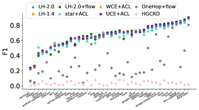
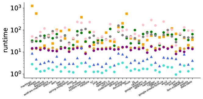
Figure 3. The upper plot shows median F1 scores of different methods over 40 clusters from the Stack Overflow dataset. The lower plot shows median running time. LH-2.0 achieves the best balance between speed and accuracy; LH-1.4 can sometimes be slower than the flow method when the target cluster contains many large hyperedges.

Table 3. This table summarizes the median of median runtimes in seconds for the Stack Overflow experiments as well as median Precision, Recall and F1 over the 40 clusters.

Alg.	LH2	LH1.4	LH2	ACL	ACL	ACL	Flow	HG-
			+flow	+star	+WCE	+UCE	+1Hop	CRD
Time	3.69	39.89	43.84	1.54	15.25	13.71	48.28	72.31
Pr	0.65	0.66	0.74	0.66	0.65	0.66	0.83	0.46
Rc	0.67	0.67	0.59	0.6	0.66	0.65	0.11	0.01
F1	0.66	0.66	0.66	0.63	0.65	0.65	0.19	0.02

7.3. Varying Number of Seeds

Comparing to the flow-based method, an advantage of our diffusion method is that it expands from a small seed set into a good enough cluster that detects many labels correctly. Now, we use the Amazon dataset to elaborate on this point. We vary the ratio of seed set from 0.1% to 10%. At each seed ratio, denoted as $r$, we set $\kappa=0.025r$. And for each of the 6 clusters, we take the median F1 score over 10 trials. To have a global idea of how different methods perform on this dataset, we take another median over the 6 median F1 scores. For the flow-based method, we also consider removing the OneHop growing procedure. The results are summarized in Figure 4. We can see our hypergraph diffusion based method (LH-1.4, LH-2.0) performs better than alternatives for all seed sizes, although flow dramatically improves for large seed sizes.

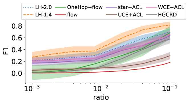
Figure 4. This plot shows the median of median F1 scores on detecting those 6 clusters in the Amazon data when varying the seed size. The envelope represents 1 standard error over the 6 median F1 scores. Without OneHop, the flow based method is not able to grow from seed set even for the largest seeds. Our hypergraph diffusion (LH) methods outperforms others, especially for small seeds.

8. DISCUSSION

This paper studies the opportunities for strongly local quadratic and $p$-norm diffusions in the context of local clustering and semi-supervised learning.

One of the distinct challenges we encountered in preparing this manuscript was comparing against the ideas of others. Clique expansions are often problematic because they can involve quadratic memory for each hyperedge if used simplistically. For running the baseline ACL PageRank diffusion on the clique expansion, we were able to use the linear nature of this algorithm to implicitly model the clique expansion without realizing the actual graph in memory. (We lack space to describe this though.) For others the results were less encouraging. We, for instance, were unable to set integration parameters for the Euler scheme employed by QHPR (Takai et al., 2020) to produce meaningful results in §7.

Consequently, we wish to discuss the parameters of our method and why they are reasonably easy to set. The values $\gamma$ and $\kappa$ both control the size of the result. Roughly, $\gamma$ corresponds to how much the diffusion is allowed to spread from the seed vertices and $\kappa$ controls how aggressively we sparsify the diffusion. To get a bigger result, then, set $\gamma$ or $\kappa$ a little bit smaller. The value of $\rho$ corresponds only to how much one of our solutions can differ from the unique solution of (6). Fixing $\rho=0.5$ is fine for empirical studies unless the goal is to compare against other strategies to solve that same equation. The final parameter is $\delta$, which interpolates between the all-or-nothing penalty and the cardinality penalty as discussed in §3.2. This can be chosen based on an experiment as we did here, or by exploring a few small choices between $1$ and half the largest hyperedge size.

In closing, flow-based algorithms have often been explained or used as refinement operations to the clusters produced by spectral methods (Lang, 2005) as in LH-2.0+flow. As a final demonstration of this usage on the Yelp experiment from §1, we have precision, recall, and F1 result of $0.87,0.998,0.93$, respectively, which demonstrates how these techniques may be easily combined to even more accurately find target clusters.

Appendix A Proof of Theorem 3.5

First we have the following observations on $\boldsymbol{\mathrm{r}}$ and $\boldsymbol{\mathrm{x}}$.

Lemma A.1.

At any iteration of Algorithm 1, for each pair of auxiliary nodes, $a\in V_{a}$, $b\in V_{b}$ and $a\rightarrow b$, $x_{a}\geq x_{b}$.

Proof.

If $x_{a}<x_{b}$, from equation (8), $r_{b}=0$ means $x_{b}\leq x_{i}$ for any $b\rightarrow i$. But this means $r_{a}>0$, which is a contradiction. ∎

Lemma A.2.

At any iteration of Algorithm 1, for any $i\in V\cup V_{a}\cup V_{b}$, $g_{i}$ will stay nonnegative and $0\leq x_{i}\leq 1$.

Proof.

The nonnegativity of $g_{i}$ is obvious. At any iteration of Algorithm 1, we either change $g_{i}$ to $\rho\kappa d_{i}$ or add some nonnegative values to the residual of adjacent nodes or keep $g_{i}$ as zero. For each original node $i\in V$, to prove $0\leq x_{i}\leq 1$, recall $r_{i}=g_{i}$ expands to (7). Suppose $x_{i}$ is the largest element and $x_{i}>1$, then $\text{Ind}(i\in R)-x_{i}<0$. Since $g_{i}\geq 0$, this means there exists $b\in V_{b}$ such that $x_{b}>x_{i}>1$. Assume $a\in V_{a}$ is adjacent to $b$, then from equation (8), $g_{a}=g_{b}=0$. Since $x_{i}$ is the largest among all nodes $i\in V$, the only way to satisfy both equations is $x_{a}=x_{b}=x_{i}$. Thus, we have $x_{i}=x_{b}>x_{i}$, which is a contradiction. To prove $x_{i}\leq 1$ for $i\in V_{a}\cup V_{b}$, from Lemma A.1, we only need to show $x_{i}\leq 1$ for $i\in V_{a}$. If there exists $a\in V_{a}$, $x_{a}>1$, since $x_{i}\leq 1$ for any $i\in V$, then $g_{a}=0$ means $x_{a}=x_{b}>1$ where $a\rightarrow b$. This means $g_{b}<0$, which is a contradiction. ∎

Proof of Theorem 3.5. By using Lemma A.2, $\|\boldsymbol{\mathrm{g}}\|_{1}$ becomes

$$\textstyle\|\boldsymbol{\mathrm{g}}\|_{1}=\sum_{i\in V\cup V_{a}\cup V_{b}}g_{i}=\sum_{i\in R}d_{i}(1-x_{i})-\sum_{i\in\bar{R}}d_{i}x_{i}$$

This implies that any change to the auxiliary nodes will not affect $||\boldsymbol{\mathrm{g}}||_{1}$. Thus calling LHQD-auxpush doesn’t change $||\boldsymbol{\mathrm{g}}||_{1}$. When there exists $i\in V$ such that $g_{i}>\kappa d_{i}$, then hyper-push will find $\Delta x_{i}$ such that $g^{\prime}_{i}=\rho\kappa d_{i}$. Then the new $g^{\prime}_{i}$ can be written as

(14) $$g_{i}^{\prime}=\frac{1}{\gamma}\sum_{b\in V_{b}}w_{bi}(x_{b}-x_{i}-\Delta x_{i})_{+}-\frac{1}{\gamma}\sum_{a\in V_{a}}w_{ia}(x_{i}+\Delta x_{i}-x_{a})_{+}+\\ \kappa d_{i}(\text{Ind}[i\in R]-x_{i}-\Delta x_{i})$$

Note $g_{i}^{\prime}$ is a decreasing function of $\Delta x_{i}$ and $g_{i}^{\prime}>0$ when $\Delta x_{i}=0$, $g_{i}^{\prime}<0$ when $\Delta x_{i}=1$ by using Lemma A.2. This suggests that there exists a unique $\Delta x_{i}$ that satisfies $g_{i}^{\prime}=\rho\kappa d_{i}$. Moreover, $(x_{b}-x_{i}-\Delta x_{i})_{+}\geq(x_{b}-x_{i})_{+}-\Delta x_{i}$ and $(x_{i}+\Delta x_{i}-x_{a})_{+}\leq(x_{i}-x_{a})_{+}+\Delta x_{i}$, thus we have

$$\textstyle\rho\kappa d_{i}=g_{i}^{\prime}\geq g_{i}-\frac{1}{\gamma}(\sum_{b\in V_{b}}w_{bi}+\sum_{a\in V_{a}}w_{ia})\Delta x_{i}-\kappa d_{i}\Delta x_{i}$$

From equation (4.9) of (Veldt et al., 2020a),

$$\textstyle\sum_{b\in V_{b}}w_{bi}=\sum_{a\in V_{a}}w_{ai}=\sum_{e\in\mathcal{E},i\in e}f_{e}(\{i\})\leq\delta d_{i}$$

Thus, we have $\textstyle d_{i}\Delta x_{i}\geq\frac{g_{i}-g_{i}^{\prime}}{\kappa+\delta/\gamma}>\frac{\gamma\kappa(1-\rho)}{\gamma\kappa+\delta}d_{i}$ So the decrease of $||\boldsymbol{\mathrm{g}}||_{1}$ will be at least $\gamma\kappa(1-\rho)d_{i}/(\gamma\kappa+\delta)$. Since $||\boldsymbol{\mathrm{g}}||_{1}=\text{vol}(R)$ initially, we have $\textstyle\sum_{i=1}^{T}d_{i}\leq(\gamma\kappa+\delta)\text{vol}(R)/\gamma\kappa(1-\rho)=O(\text{vol}(R))$.

Appendix B Proof of Theorem 4.2

We first introduce some simplifying notation. We use $1_{v}$ to denote the canonical basis with $v$th component as 1 and others as 0 and $1_{S}=\sum_{v\in S}1_{v}$. Without loss of generality, we assume each gadget reduced from a hyperedge has weight $c_{e}=1$. Otherwise one can simply add $c_{e}$ as the coefficients and nothing needs to change. We omit the degree regularization term in (6). Furthermore, we normalize the seeds to guarantee $\sum_{v\in V}d_{v}x_{v}=1$ and group terms in (6) to remove the source $x_{s}=1$ and sink $x_{t}=0$

(15) $$\operatorname*{minimize}_{\boldsymbol{\mathrm{x}}}\quad Q(\boldsymbol{\mathrm{x}})\triangleq\gamma\sum_{v\in V}d_{v}\left(x_{v}-\frac{1}{\textbf{vol}(S)}1_{S}\right)^{2}+\sum_{e\in\mathcal{E}}Q_{e}(\boldsymbol{\mathrm{x}})$$

where

(16) $$\footnotesize Q_{e}(\boldsymbol{\mathrm{x}})\triangleq\underset{x_{a}^{(e)},x_{b}^{(e)}}{\min}\sum_{v\in e}\left[(x_{v}-x_{a}^{(e)})_{+}^{2}+(x_{b}^{(e)}-x_{v})_{+}^{2}\right]+\delta_{e}(x_{a}^{(e)}-x_{b}^{(e)})_{+}^{2}.$$

We denote $M=\textbf{vol}(\mathcal{H})=\sum_{v\in V}d_{v}$. We denote the solution $\boldsymbol{\mathrm{x}}$ with the parameter $\gamma$ and the seed set $S$ of the optimization (15) as $\boldsymbol{\mathrm{x}}(\gamma,S)$ and its component for node $v$ as $x_{v}(\gamma,S)$. We also define another degree weighted vector $p=D\boldsymbol{\mathrm{x}}$, where $D$ is the diagonal degree matrix. For a vector $p$ and a node set $S^{\prime}$, we use $p(S^{\prime})$ to denote $p(S^{\prime})=\sum_{v\in S^{\prime}}p_{v}$. It is easy to check that $p(\gamma,S)(V)=1$ for any $S$. For a node set $S$, define $\partial S=\{e\in\mathcal{E}|e\cap S\neq\emptyset,e\cap V\backslash S\neq\emptyset\}$.

We now define our main tool: the Lovász-Simonovits Curve.

Definition B.1 (Lovász-Simonovits Curve (LSC)).

Given an $\boldsymbol{\mathrm{x}}$, we order its components from large to small by breaking equality arbitrarily, say $x_{1},x_{2},....,x_{n}$ w.l.o.g, and define $S_{j}^{\boldsymbol{\mathrm{x}}}=\{x_{1},...,x_{j}\}$. LSC defines a corresponding piece-wise function $I_{\boldsymbol{\mathrm{x}}}:[0,M]\rightarrow R$ s.t $I_{\boldsymbol{\mathrm{x}}}(0)=0$, $I_{\boldsymbol{\mathrm{x}}}(\textbf{vol}(G))=1$ and $I(\textbf{vol}(S_{j}^{\boldsymbol{\mathrm{x}}}))=p(S_{j}^{\boldsymbol{\mathrm{x}}}).$ And for any $k\in[\textbf{vol}(S_{j}^{\boldsymbol{\mathrm{x}}}),\textbf{vol}(S_{j+1}^{\boldsymbol{\mathrm{x}}})]$,

$$I_{\boldsymbol{\mathrm{x}}}(k)=I_{\boldsymbol{\mathrm{x}}}(\textbf{vol}(S_{j}^{\boldsymbol{\mathrm{x}}}))+(k-\textbf{vol}(S_{j}^{\boldsymbol{\mathrm{x}}}))x_{j}.$$

Our proof depends on the following two Lemma B.2 and B.3 that will characterize the upper and lower bound of $I_{\boldsymbol{\mathrm{x}}}$, which finally leads to the main theorem.

Lemma B.2.

For a set $S$, given an $\boldsymbol{\mathrm{x}}=\boldsymbol{\mathrm{x}}(\gamma,S)$, let $\phi_{\boldsymbol{\mathrm{x}}}$ and $S_{\boldsymbol{\mathrm{x}}}$ be the minimal conductance and the node set obtained through a sweep-cut over $\boldsymbol{\mathrm{x}}$. For any integer $t>0$ and $k\in[0,M]$, the following bound holds

$$I_{\boldsymbol{\mathrm{x}}}(k)\leq\frac{k}{M}+\frac{\gamma t}{2+\gamma}+\sqrt{\frac{\min(k,M-k)}{\min_{i\in S}d_{i}}}(1-\frac{\sigma_{\boldsymbol{\mathrm{x}}}^{2}\phi_{\boldsymbol{\mathrm{x}}}^{2}}{8})^{t}$$

where $\sigma_{\boldsymbol{\mathrm{x}}}=(2\max_{e\in\partial S_{\boldsymbol{\mathrm{x}}}}\min\{\delta_{e},|e|/2\}+1)^{-1}$.

Lemma B.3.

For a set $S$, if a node $v\in S$ is sampled according to a distribution $\mathbb{P}$ s.t

(17) $$\mathbb{E}_{v\sim\mathbb{P}}[p(\gamma,\{v\})(\bar{S})]\leq cp(\gamma,S)(\bar{S}),$$

where $c$ is a constant, then with probability at least $\frac{1}{2},$ one has

$$p(\gamma,\{v\})(S)\geq 1-{2c\phi(S)}/{\gamma}.$$

Lemma B.3 gives the lower bound $I_{\boldsymbol{\mathrm{x}}(\gamma,\{v\})}(\textbf{vol}(S))$ as this value is no less than $p(\gamma,\{v\})(S)$. Note that the sampling assumption of Lemma B.3 is natural in the standard graph case, when $\mathbb{P}$ samples each node proportionally to its degree, we have an equality with $c=1$ in (17). Combining Lemma B.2 and B.3, we arrive at

Theorem B.4.

Given a set $S^{*}$ of vertices s.t. $\textbf{vol}(S^{*})\leq\frac{M}{2}$ and $\phi(S^{*})\leq\frac{\gamma}{8c}$ for some positive constants $\gamma,\,c.$ If there exists a distribution $\mathbb{P}$ s.t. $\mathbb{E}_{v\sim\mathbb{P}}[p(\gamma,\{v\})](\bar{S}^{*})\leq cp(\gamma,S^{*})(\bar{S}^{*}),$ then with probability at least $\frac{1}{2},$ the obtained conductance satisfies

$$\phi_{\boldsymbol{\mathrm{x}}}\leq\sqrt{32\gamma\max_{e\in\partial S_{\boldsymbol{\mathrm{x}}}}\min\left\{\delta_{e},\frac{|e|}{2}\right\}ln\left(100\frac{\textbf{vol}(S^{*})}{d_{v}}\right)},$$

where $\boldsymbol{\mathrm{x}}=\boldsymbol{\mathrm{x}}(\gamma,\{v\})$ and $v$ is sampled from $\mathbb{P}$. $S_{\boldsymbol{\mathrm{x}}}$ is the node set obtained via the sweep-cut over $\boldsymbol{\mathrm{x}}$.

Proof.

We combine Lemma B.3 and B.2 and use the same technique as Thm. 17 in (Li et al., 2020) (Sec. 7.7.3). ∎

By removing the normalizing on the number of seeded nodes, Thm. B.4 becomes Thm. 4.2.

B.1. Proof of Lemma B.2

Define $L_{e}(\boldsymbol{\mathrm{x}})\triangleq\nabla_{\boldsymbol{\mathrm{x}}}\frac{1}{2}Q_{e}(\boldsymbol{\mathrm{x}})$ (16) and with some algebra, we have

$$L_{e}(\boldsymbol{\mathrm{x}})=\sum_{v\in e}\left[(x_{v}-x_{a}^{(e)*})_{+}-(x_{b}^{(e)*}-x_{v})_{+}\right]1_{v},$$

where $x_{a}^{(e)*}$ and $x_{b}^{(e)*}$ are the optimal values in (16). In the following, we will first prove Lemma B.5 and further use it to prove Lemma B.6. The same proof in Thm. 16 in (Li et al., 2020) (Sec. 7.7.2) can be used to leverage Lemma B.6 to prove Lemma B.2.

Lemma B.5.

Given an $\boldsymbol{\mathrm{x}}$, we order its components from large to small, say $x_{1},x_{2},....,x_{n}$ w.l.o.g., and define $S_{j}^{\boldsymbol{\mathrm{x}}}=\{x_{1},...,x_{j}\}$. Define $\sigma_{j}^{\boldsymbol{\mathrm{x}}}=(1+2\max_{e\in\partial S_{j}^{\boldsymbol{\mathrm{x}}}}\min\left\{\delta_{e},|e|/2\right\})^{-1},$ and we have

$$2I_{\boldsymbol{\mathrm{x}}}(\textbf{vol}(S_{j}^{\boldsymbol{\mathrm{x}}}))-\langle\sum_{e\in E}L_{e}(x),1_{S_{j}^{\boldsymbol{\mathrm{x}}}}\rangle \leq$$

$$I_{\boldsymbol{\mathrm{x}}}(\textbf{vol}(S_{j}^{\boldsymbol{\mathrm{x}}})-\sigma_{j}^{\boldsymbol{\mathrm{x}}}cut(S_{j}^{\boldsymbol{\mathrm{x}}})) +I_{\boldsymbol{\mathrm{x}}}(\textbf{vol}(S_{j}^{\boldsymbol{\mathrm{x}}})+\sigma_{j}^{\boldsymbol{\mathrm{x}}}cut(S_{j}^{\boldsymbol{\mathrm{x}}})).$$

Lemma B.6.

Suppose $\boldsymbol{\mathrm{x}}=\boldsymbol{\mathrm{x}}(\gamma,S)$, $\boldsymbol{\mathrm{x}}_{0}=1_{S}/\textbf{vol}(S)$ and $\sigma_{j}^{\boldsymbol{\mathrm{x}}}=(1+2\max_{e\in\partial S_{j}^{\boldsymbol{\mathrm{x}}}}\min\{\delta_{e},|e|/2\})^{-1}$. We have

(18) $$I_{\boldsymbol{\mathrm{x}}}(\textbf{vol}(S_{j}^{\boldsymbol{\mathrm{x}}}))\leq\frac{\gamma}{2+\gamma}I_{\boldsymbol{\mathrm{x}}_{0}}(S_{j}^{\boldsymbol{\mathrm{x}}_{0}})+\frac{1}{2+\gamma}(I_{\boldsymbol{\mathrm{x}}}(\textbf{vol}(S_{j}^{\boldsymbol{\mathrm{x}}})-\sigma_{j}^{\boldsymbol{\mathrm{x}}}cut(S_{j}^{\boldsymbol{\mathrm{x}}}))+\\ I_{\boldsymbol{\mathrm{x}}}(\textbf{vol}(S_{j}^{\boldsymbol{\mathrm{x}}})+\sigma_{j}^{\boldsymbol{\mathrm{x}}}cut(S_{j}^{\boldsymbol{\mathrm{x}}}))).$$

Furthermore, for $k\in[0,M],$ $I_{\boldsymbol{\mathrm{x}}}(k)\leq I_{\boldsymbol{\mathrm{x}}_{0}}(k).$

Proof of Lemma B.5. Given a hyperedge $e$, we order $\{x_{v}\mid v\in e\}$ from large to small by breaking equality arbitrarily and obtain $x_{1}^{(e)},x_{2}^{(e)},...,x_{e}^{(e)}$. Suppose $x_{k}^{(e)}\in S_{j}^{\boldsymbol{\mathrm{x}}}$ and $x_{k+1}^{(e)}\notin S_{j}^{\boldsymbol{\mathrm{x}}}$. Then,

(19) $$\textstyle\langle L_{e}(x),1_{S_{j}^{\boldsymbol{\mathrm{x}}}}\rangle=\sum\limits_{i=1}^{k}\bigl{[}(x_{i}^{(e)}-x_{a}^{(e)*})_{+}-(x_{b}^{(e)*}-x_{i}^{(e)})_{+}\bigr{]}$$

Next, we will bound (19) by analyzing three cases. We only focus on $x_{a}^{(e)*}>x_{b}^{(e)*}$ and otherwise $x_{v}$’s are constant for all $v\in e$. Also denote $k_{+}=\max\{i\mid x_{i}^{(e)}>x_{a}^{(e)*}\}$, $k_{-}=\min\{e+1-i\mid x_{i}^{(e)}<x_{b}^{(e)*}\}$, and $k^{-}=|e|+1-k_{-}$. By the optimality of $x_{a}^{(e)*},\,x_{b}^{(e)*}$, we have

$$x_{a}^{(e)*}=(k_{-}+\delta_{e})X_{1}^{k_{+}}+\delta_{e}X_{k^{-}}^{|e|},\quad x_{b}^{(e)*}=\delta_{e}X_{1}^{k_{+}}+(k_{+}+\delta_{e})X_{k^{-}}^{|e|},$$

where $X_{i_{1}}^{i_{2}}=(k_{+}k_{-}+\delta_{e}(k_{+}+k_{-}))^{-1}\textstyle\sum_{i=i_{1}}^{i_{2}}x_{i}^{(e)}.$

Thus, we have

(20) $$\langle L_{e}(x),1_{S_{j}^{\boldsymbol{\mathrm{x}}}}\rangle\!=\!\footnotesize\left\{\begin{array}[]{@{}l@{\;\;}l@{}}[(k_{+}-k)(k_{-}+\delta_{e})+k_{-}\delta_{e}]X_{1}^{k}&\text{if}\,k\leq k_{+}\\ \quad-k(k_{-}+\delta_{e})X_{k+1}^{k_{+}}-k\delta_{e}X_{k^{-}}^{|e|},&\\ k_{-}\delta_{e}X_{1}^{k_{+}}-k_{+}\delta_{e}X_{k^{-}}^{|e|},&\text{if}\,k_{+}\leq k\leq k^{-}\\ (|e|-k)\delta_{e}X_{1}^{k_{+}}+(|e|-k)(k_{+}+\delta_{e})X_{k^{-}}^{k}&\text{if}\,k\geq k^{-}.\\ \quad-[k_{+}\delta_{e}+(k-k^{-})(k_{+}+\delta_{e})]X_{k}^{|e|}\end{array}\right.$$

By using the definition of $X_{i_{1}}^{i_{2}}$, noticing that all coefficients on $x_{i}^{(e)}\leq 1$ in the left hand side of (20), and a good deal of algebra, we can further show

$$\small\left\{\begin{array}[]{@{}ll@{}}\frac{k(k_{+}-k)(k_{-}+\delta_{e})+k_{-}\delta_{e}}{k_{+}k_{-}+\delta_{e}(k_{+}+k_{-})}\geq\frac{2}{\delta_{e}^{\prime}+2}\min\{k,|e|-k,\delta_{e}\}&\text{if}\,k\leq k_{+}\\ \frac{k_{+}k_{-}\delta_{e}}{k_{+}k_{-}+\delta_{e}(k_{+}+k_{-})}\geq\frac{1}{2\delta_{e}^{\prime}+1}\min\{k,|e|-k,\delta_{e}\},&\text{if}\,k_{+}\leq k\leq k^{-}\\ \frac{k_{-}[k_{+}\delta_{e}+(k-k^{-})(k_{+}+\delta_{e})]}{k_{+}k_{-}+\delta_{e}(k_{+}+k_{-})}\geq\frac{2}{\delta_{e}^{\prime}+2}\min\{k,|e|-k,\delta_{e}\},&\text{if}\,k\geq k^{-}.\end{array}\right.$$

where $\delta_{e}^{\prime}=\min\{\delta_{e},|e|/2\}$. In each case of (20), the sum of positive coefficient before each $x_{i}^{(e)}$ equals to the sum of negative coefficients, which are both lower bounded by $\frac{1}{2\delta_{e}^{\prime}+1}$ times the splitting cost of $e$. Therefore,

$$2I_{\boldsymbol{\mathrm{x}}}(\textbf{vol}(S_{j}^{\boldsymbol{\mathrm{x}}}))-\sum_{e\in E}\langle L_{e}(x),1_{S_{j}^{\boldsymbol{\mathrm{x}}}}\rangle \leq$$

$$I_{\boldsymbol{\mathrm{x}}}(\textbf{vol}(S_{j}^{\boldsymbol{\mathrm{x}}})-\sigma_{j}^{\boldsymbol{\mathrm{x}}}cut(S_{j}^{\boldsymbol{\mathrm{x}}})) +I_{\boldsymbol{\mathrm{x}}}(\textbf{vol}(S_{j}^{\boldsymbol{\mathrm{x}}})+\sigma_{j}^{\boldsymbol{\mathrm{x}}}cut(S_{j}^{\boldsymbol{\mathrm{x}}})),$$

where $\sigma_{j}^{\boldsymbol{\mathrm{x}}}=1/(2\max_{e\in\partial S_{j}^{\boldsymbol{\mathrm{x}}}}\delta_{e}^{\prime}+1)$, which concludes the proof.

Proof of Lemma B.6. Compute the derivative of $Q(\boldsymbol{\mathrm{x}})$ (15) w.r.t. $\boldsymbol{\mathrm{x}}$ and use the optimality of $\boldsymbol{\mathrm{x}}=\boldsymbol{\mathrm{x}}(\gamma,S)$ to get $0=\gamma D(\boldsymbol{\mathrm{x}}-\boldsymbol{\mathrm{x}}_{0})+L_{e}(\boldsymbol{\mathrm{x}})$. Therefore,the inner product with $1_{S_{j}^{\boldsymbol{\mathrm{x}}}}$

$$0=\gamma(I_{\boldsymbol{\mathrm{x}}}(\textbf{vol}(S_{j}^{\boldsymbol{\mathrm{x}}}))-I_{\boldsymbol{\mathrm{x}}_{0}}(\textbf{vol}(S_{j}^{\boldsymbol{\mathrm{x}}_{0}})))+\langle L_{e}(\boldsymbol{\mathrm{x}}),1_{S_{j}^{\boldsymbol{\mathrm{x}}}}\rangle.$$

Plug in Lemma B.5 and we achieve (18). By using the concavity of $I_{\boldsymbol{\mathrm{x}}}$, we obtain $I_{\boldsymbol{\mathrm{x}}}(\textbf{vol}(S_{j}^{\boldsymbol{\mathrm{x}}}))\leq I_{\boldsymbol{\mathrm{x}}_{0}}(\textbf{vol}(S_{j}^{\boldsymbol{\mathrm{x}}_{0}}))$ and therefore $I_{\boldsymbol{\mathrm{x}}}(k)\leq I_{\boldsymbol{\mathrm{x}}_{0}}(k)$ for any $k\in[0,M]$.

B.2. Proof of Lemma B.3

If the following Lemma B.7 is true, then we have $\mathbb{E}_{v\sim\mathbb{P}}[p(\gamma,\{v\})(\bar{S})]\leq cp(\gamma,S)(\bar{S})=c(1-p(\gamma,S)(S))\leq{c\phi(S)}/{\gamma}$. By using Markov’s inequality, with probability $\frac{1}{2}$, we will sample a node $v$ such that $p(\gamma,\{v\})(\bar{S})\leq{2c\phi(S)}/{\gamma}$, which concludes the proof.

Lemma B.7.

For any $S\subset V$, $p(\gamma,S)(S)\geq 1-{\phi(S)}/{\gamma}$.

Proof. This mass from the nodes in $S$ to the nodes in $\bar{S}$ naturally diffuses from the auxiliary nodes $v_{a}^{(e)}$ to $v_{b}^{(e)}$ for $e\in\partial S$. As need to lower bound $p(\gamma,S)(S)$, we may consider fixing $x_{v}=0,\forall v\in\bar{S}$ of $Q(\boldsymbol{\mathrm{x}})$ and the obtained solution $\tilde{\boldsymbol{\mathrm{x}}}$ naturally satisfies

$$p(\gamma,S)(S)\geq\sum\nolimits_{v\in S}d_{v}\tilde{x}_{v},\;\text{where}\;\tilde{\boldsymbol{\mathrm{x}}}\triangleq\arg\min_{\boldsymbol{\mathrm{x}}}Q(\boldsymbol{\mathrm{x}})|_{x_{v}=0,\forall v\in\bar{S}}.$$

The optimality of $\tilde{x}_{a}^{(e)},\tilde{x}_{b}^{(e)}$ for $e\in\partial S$ in this case implies

$$\textstyle-\sum_{v\in e}(\tilde{x}_{v}-\tilde{x}_{a}^{(e)})_{+}+\delta_{e}(\tilde{x}_{a}^{(e)}-\tilde{x}_{b}^{(e)})_{+}=0,$$

$$\textstyle\sum_{v\in e}(-\tilde{x}_{v}+\tilde{x}_{b}^{(e)})_{+}-\delta_{e}(\tilde{x}_{a}^{(e)}-\tilde{x}_{b}^{(e)})_{+}=0$$

As $\tilde{x}_{v}=0$ for $v\in e\backslash S$ and $\tilde{x}_{v}\leq\frac{1}{\textbf{vol}(S)}$ for $v\in e\cap S$, we have

$$\tilde{x}_{b}^{(e)}\geq\frac{\delta_{e}}{\delta_{e}+|e\backslash S|}\tilde{x}_{a}^{(e)},\;\tilde{x}_{a}^{(e)} \leq\frac{|e\cap S|}{\delta_{e}+|e\cap S|}\frac{1}{\textbf{vol}(S)},$$

and further, $\forall e\in\partial S$,

(21) $$\textstyle\sum_{v\in e\cap S}(\tilde{x}_{v}-\tilde{x}_{a}^{(e)})_{+}=\delta_{e}(\tilde{x}_{a}^{(e)}-\tilde{x}_{b}^{(e)})_{+}$$

$$\leq\frac{|e\cap S||e\backslash S|\delta_{e}}{(\delta_{e}+|e\cap S|)(\delta_{e}+|e\backslash S|)}\frac{1}{\textbf{vol}(S)}\leq\frac{\min\{|e\cap S|,|e\backslash S|,\delta_{e}\}}{\textbf{vol}(S)}.$$

The optimality of $\tilde{\boldsymbol{\mathrm{x}}}$ implies

(22) $$\sum_{v\in S}\gamma d_{v}\left(\tilde{x}_{v}-\frac{1}{\textbf{vol}(S)}\right)+\sum_{e\in\partial S}\sum_{v\in e\cap S}(\tilde{x}_{v}-\tilde{x}_{a}^{(e)})_{+}=0.$$

Here we use that $\sum_{e\subset S}\sum_{v\in e}[(\tilde{x}_{v}-\tilde{x}_{a}^{(e)})_{+}+(\tilde{x}_{b}^{(e)}-\tilde{x}_{v})_{+}]=0$. Plug (21) into (22) and we have

$$0\!\leq\!\gamma\left(\sum_{v\in S}d_{v}\tilde{x}_{v}-1\right)+\cancelto{\phi(S)}{\sum_{e\in\partial S}\frac{\min\{|e\cap S|,|e\backslash S|,\delta_{e}\}}{\textbf{vol}(S)}},$$

which concludes the proof.

Appendix C Selecting $\delta$.

To select $\delta$ for each dataset, we run LH-2.0 on a handful of alternative clusters as we vary $\delta$. Below, we show F1 scores on those clusters and pick $\delta=1$ for Amazon and $\delta=1000$ for Stack Overflow.

References

- (1)
- Agarwal et al. (2006) Sameer Agarwal, Kristin Branson, and Serge Belongie. 2006. Higher Order Learning with Graphs. In ICML. 17–24.
- Agarwal et al. (2005) Sameer Agarwal, Jongwoo Lim, Lihi Zelnik-Manor, Pietro Perona, David Kriegman, and Serge Belongie. 2005. Beyond Pairwise Clustering. In CVPR. 838–845.
- Andersen et al. (2006) Reid Andersen, Fan Chung, and Kevin Lang. 2006. Local graph partitioning using pagerank vectors. In FOCS. 475–486.
- Andersen and Lang (2008) Reid Andersen and Kevin J. Lang. 2008. An Algorithm for Improving Graph Partitions. In SODA. 651–660.
- Benson et al. (2016) Austin Benson, David F. Gleich, and Jure Leskovec. 2016. Higher-order organization of complex networks. Science 353 (2016), 163–166.
- Benson et al. (2020) Austin R Benson, Jon Kleinberg, and Nate Veldt. 2020. Augmented Sparsifiers for Generalized Hypergraph Cuts. arXiv preprint arXiv:2007.08075 (2020).
- Blum and Chawla (2001) Avrim Blum and Shuchi Chawla. 2001. Learning from Labeled and Unlabeled Data Using Graph Mincuts. In ICML. 19–26.
- Chitra and Raphael (2019) Uthsav Chitra and Benjamin J. Raphael. 2019. Random Walks on Hypergraphs with Edge-Dependent Vertex Weights. In ICML. 1172–1181.
- Chung (1992) Fan R. L. Chung. 1992. Spectral Graph Theory. American Mathematical Society.
- Eckles et al. (2017) D. Eckles, B. Karrer, and J. Ugander. 2017. Design and Analysis of Experiments in Networks: Reducing Bias from Interference. J. Causal Inference 5 (2017).
- Fountoulakis et al. (2020) K. Fountoulakis, M. Liu, D. F. Gleich, and M. W. Mahoney. 2020. Flow-based Algorithms for Improving Clusters: A Unifying Framework, Software, and Performance. arXiv cs.LG (2020), 2004.09608.
- Gleich and Mahoney (2014) David Gleich and Michael Mahoney. 2014. Anti-differentiating approximation algorithms: A case study with min-cuts, spectral, and flow. In ICML. 1018–1025.
- Gleich and Mahoney (2015) David F. Gleich and Michael W. Mahoney. 2015. Using Local Spectral Methods to Robustify Graph-Based Learning Algorithms. In SIGKDD. 359–368.
- Hadley (1995) Scott W. Hadley. 1995. Approximation techniques for hypergraph partitioning problems. Discrete Applied Mathematics 59, 2 (1995), 115 – 127.
- Hein et al. (2013) M. Hein, S. Setzer, L. Jost, and S. S. Rangapuram. 2013. The Total Variation on Hypergraphs - Learning on Hypergraphs Revisited. In NeurIPS. 2427–2435.
- Ibrahim and Gleich (2019) Rania Ibrahim and David F. Gleich. 2019. Nonlinear Diffusion for Community Detection and Semi-Supervised Learning. In The World Wide Web Conference (San Francisco, CA, USA) (WWW ’19). ACM, New York, NY, USA, 739–750.
- Ibrahim and Gleich (2020) Rania Ibrahim and David F. Gleich. 2020. Local Hypergraph Clustering using Capacity Releasing Diffusion. arXiv cs.SI (2020), 2003.04213.
- Ihler et al. (1993) E. Ihler, D. Wagner, and F. Wagner. 1993. Modeling hypergraphs by graphs with the same mincut properties. Inform. Process. Lett. 45 (1993), 171–175.
- Joachims (2003) T. Joachims. 2003. Transductive learning via spectral graph partitioning. In ICML. 290–297.
- Karypis et al. (1999) G. Karypis, R. Aggarwal, V. Kumar, and S. Shekhar. 1999. Multilevel hypergraph partitioning: applications in VLSI domain. VLSI 7, 1 (March 1999), 69–79.
- Lang (2005) K. Lang. 2005. Fixing two weaknesses of the spectral method. In NeurIPS. 715–722.
- Lawler (1973) E. L. Lawler. 1973. Cutsets and partitions of hypergraphs. Networks 3, 3 (1973), 275–285.
- Lawlor et al. (2016) D. Lawlor, T. Budavári, and M. W Mahoney. 2016. Mapping the Similarities of Spectra: Global and Locally-biased Approaches to SDSS Galaxies. Astrophys. J. 833, 1 (2016), 26.
- Leskovec et al. (2009) J. Leskovec, K. J. Lang, A. Dasgupta, and M. W. Mahoney. 2009. Community Structure in Large Networks: Natural Cluster Sizes and the Absence of Large Well-Defined Clusters. Internet Math. 6, 1 (2009), 29–123.
- Li et al. (2020) Pan Li, Niao He, and Olgica Milenkovic. 2020. Quadratic Decomposable Submodular Function Minimization: Theory and Practice. JMLR 21 (2020), 1–49.
- Li and Milenkovic (2017) Pan Li and Olgica Milenkovic. 2017. Inhomogeneous Hypergraph Clustering with Applications. In NeurIPS. 2308–2318.
- Li and Milenkovic (2018) Pan Li and Olgica Milenkovic. 2018. Submodular Hypergraphs: p-Laplacians, Cheeger Inequalities and Spectral Clustering. In ICML, Vol. 80. 3014–3023.
- Liu and Gleich (2020) Meng Liu and David F. Gleich. 2020. Strongly local p-norm-cut algorithms for semi-supervised learning and local graph clustering. arXiv:2006.08569 [cs.SI]
- Mahoney et al. (2012) M. W. Mahoney, L. Orecchia, and N. K. Vishnoi. 2012. A Local Spectral Method for Graphs: With Applications to Improving Graph Partitions and Exploring Data Graphs Locally. JMLR 13 (2012), 2339–2365.
- Ni et al. (2019) Jianmo Ni, Jiacheng Li, and Julian McAuley. 2019. Justifying Recommendations using Distantly-Labeled Reviews and Fine-Grained Aspects. In EMNLP-IJCNLP.
- Takai et al. (2020) Yuuki Takai, Atsushi Miyauchi, Masahiro Ikeda, and Yuichi Yoshida. 2020. Hypergraph Clustering Based on PageRank. In KDD. 1970–1978.
- Veldt et al. (2020a) Nate Veldt, Austin R. Benson, and Jon Kleinberg. 2020a. Hypergraph Cuts with General Splitting Functions. arXiv:2001.02817 [cs.DS]
- Veldt et al. (2020b) Nate Veldt, Austin R Benson, and Jon Kleinberg. 2020b. Minimizing Localized Ratio Cut Objectives in Hypergraphs. In KDD. 1708–1718.
- Veldt et al. (2016) Nate Veldt, David F. Gleich, and Michael W. Mahoney. 2016. A Simple and Strongly-Local Flow-Based Method for Cut Improvement. In ICML. 1938–1947.
- Veldt et al. (2019) Nate Veldt, Christine Klymko, and David F. Gleich. 2019. Flow-Based Local Graph Clustering with Better Seed Set Inclusion. In SDM. 378–386.
- Wang et al. (2017) D. Wang, K. Fountoulakis, M. Henzinger, M. W. Mahoney, and S. Rao. 2017. Capacity releasing diffusion for speed and locality. In ICML. 3598–3607.
- Yang et al. (2020) Shenghao Yang, Di Wang, and Kimon Fountoulakis. 2020. -Norm Flow Diffusion for Local Graph Clustering. arXiv preprint arXiv:2005.09810 (2020).
- Yin et al. (2017) Hao Yin, Austin R. Benson, Jure Leskovec, and David F. Gleich. 2017. Local Higher-Order Graph Clustering. In KDD. 555–564.
- Yoshida (2016) Yuichi Yoshida. 2016. Nonlinear Laplacian for digraphs and its applications to network analysis. In WSDM. 483–492.
- Yoshida (2019) Yuichi Yoshida. 2019. Cheeger Inequalities for Submodular Transformations. In SODA. 2582–2601.
- Zhang et al. (2017) Chenzi Zhang, Shuguang Hu, Zhihao Gavin Tang, and T-H. Hubert Chan. 2017. Re-Revisiting Learning on Hypergraphs: Confidence Interval and Subgradient Method. In ICML. 4026–4034.
- Zhou et al. (2003) Dengyong Zhou, Olivier Bousquet, Thomas Navin Lal, Jason Weston, and Bernhard Schölkopf. 2003. Learning with Local and Global Consistency. In NIPS.
- Zhou et al. (2006) Dengyong Zhou, Jiayuan Huang, and Bernhard Schölkopf. 2006. Learning with Hypergraphs: Clustering, Classification, and Embedding. In NeurIPS. 1601–1608.
- Zhu et al. (2003) Xiaojin Zhu, Zoubin Ghahramani, and John Lafferty. 2003. Semi-Supervised Learning Using Gaussian Fields and Harmonic Functions. In ICML. 912–919.
- Zhu et al. (2013) Zeyuan Allen Zhu, Silvio Lattanzi, and Vahab S Mirrokni. 2013. A Local Algorithm for Finding Well-Connected Clusters.. In ICML (3). 396–404.
- Zien et al. (1999) J. Y. Zien, M. D. F. Schlag, and P. K. Chan. 1999. Multilevel spectral hypergraph partitioning with arbitrary vertex sizes. IEEE TCAD 18, 9 (1999), 1389–1399.