Cryogenic spin Seebeck effect

Abstract

We present a theory of the non-linearities of the spin Seebeck effect (SSE) in a ferromagnetic nanowire at cryogenic temperatures. We adopt a microscopic quantum noise model based on a collection of two-level systems. At certain positions of Pt detectors to the wire, the transverse SSE changes sign as a function of temperature and/or temperature gradient. On the other hand, the longitudinal SSE does not show significant non-linearities even far outside the regime of validity of linear response theory.

We address the spin Seebeck effect (SSE) in electrically insulating magnets, i.e. the spin current caused by a temperature gradient as detected by the inverse spin Hall effect voltage in heavy metal contacts [2, 4, 5, 6, 7, 8, 9]. The longitudinal SSE (LSSE) is observed in a planar configuration in which the heat and spin currents flow in parallel and normal to the interfaces [10]. The transverse or non-local [11] SSE (TSSE) refers to more complicated configurations, usually two contacts on the surface of a magnetic slab or film. The spin current is injected into the metal contact by spin pumping [4] but the signal is usually dominated by the currents that are generated by temperature gradients in the bulk of the magnet [12]. The reported signals are in general proportional to the applied temperature differences $\triangle T.$ However, several recent studies of the SSE at low temperatures [13, 14, 16, 15, 17, 18, 19, 20] do not address a fundamental issue of thermal transport at ultralow temperatures. Linear response is valid when the perturbation is sufficiently small, but the properly normalized driving force is not $\triangle T$ but $\triangle T/T$ (or $\partial T/T),$ i.e. the temperature difference divided by the average one [21]. This condition is increasingly difficult to fulfill at low temperatures, or positively formulated, it should become easier to access non-linear thermomagnonic transport phenomena.

Existing theoretical treatments of the spin Seebeck effect are not suitable to address the low-temperature and non-linear regimes. The low frequency magnons that dominate at cryogenic temperatures are strongly affected by dipolar interactions, so exchange-only magnon models fail. The assumption of a semiclassical magnon accumulation in terms of a local chemical potential and magnon temperature [22] breaks down because thermalization becomes weak. With a classical magnetization noise model and in linear response, the non-thermal distribution functions governing the SSE can be described by mode- (rather than position-) dependent magnon temperatures and chemical potentials [24]. Treatments of the stochastic magnetization dynamics in terms of classical white noise sources [26, 27, 25, 28] do not work at low temperatures. This can be repaired by a noise spectrum that obeys the quantum fluctuation dissipation theorem [29], but at the cost of introducing phenomenological damping constants. A recent linear response study of the LSSE at low temperatures [31] focuses on the magnon-polaron hybrid state at large magnetic fields [30].

The broadening of the ferromagnetic resonance of a YIG sphere increases $\propto T$ for $T>1\,$K. The minimum in the damping followed by an increase and saturation with decreasing temperatures $<1\,$K [32] is caused by impurities and disorder, presumably two-level systems (TLS) [34, 35, 33]. The spin and heat transport in this regime has to our knowledge not been addressed in the literature and is the focus of this Letter. We study the cryogenic SSE of a ferromagnetic (FM) nanowire with a microscopic TLS model for the thermal noise at weak magnetic fields. In this regime magnon-magnon and magnon-phonon interactions may be safely disregarded. We predict that the antisymmetry of the TSSE signal as a function of position of a Pt detector [4, 5, 26] is broken in the non-linear regime and a non-monotonous temperature dependence at certain contact positions emerges. These effects are caused by the non-uniform gradient of the spin distribution functions in spite of a constant temperature gradient. The LSSE signal is on the other hand surprisingly robust, with a linear dependence on a global temperature difference $\Delta T$ much larger than $T_{M}$.

Model. We consider YIG nanostructures with high quality surfaces [36] in which scattering at low temperatures is dominated by rare earth (RE) substitutional impurities, e.g. Tb or Yb, on the Y sites [32, 34, 35, 33]. Two degenerate atomic levels of a RE atom form a two-level system (TLS) with pseudo-spin $\vec{\Omega}$ that interacts with the local iron magnetic moments of spin $\vec{S}_{Fe}$ by an exchange interaction $H_{TLS}=\vec{S}_{Fe}\cdot\bar{K}\vec{\Omega}$, where $\bar{K}$ is an anisotropic exchange interaction tensor, which splits the pseudo-spin levels by $\omega_{01}$. Since the RE angular momentum strongly couples to the lattice, spin waves can be efficiently dissipated via $H_{TLS}$. The isotropic Heisenberg exchange contribution $S_{x(y)}\Omega_{x(y)}$ couples the precessional dynamics and leads to a “transverse” relaxation that preserves the total magnetization. The anisotropy introduces “longitudinal” terms like $S_{x}\Omega_{z}$ and $S_{y}\Omega_{z}$ by which the splitting $\omega_{01}$ depends on the magnetization direction. Van Vleck [35, 33] computed the life time broadenings due to $H_{TLS}$ as a function of the ratio of rare earth to Fe concentration $c$. For the longitudinal process he reports

Figure 1: Model. (a) The dissipation caused by two TLS ensembles that fit the experiments of Tabuchi et al. [32]. $\Gamma_{tot}=\sum_{j=1,2}\Gamma_{L(T),j}$, where $j$ indicates the ensembles parametrized by $c_{1}=3\times 10^{-7}$, $c_{2}=1\times 10^{-4}$, $\tau_{1}=10\,$ns, $\tau_{2}=0.1\,$ps, $\omega_{1,01}=2\pi\times 10\,$GHz, $\omega_{2,01}=2\pi\times 150\,$GHz and $\omega_{U}=2\pi\times 10\,$GHz. (b) A spin Seebeck current $\mathcal{J}^{(s)}$ polarized along $\hat{z}$ flows from the magnet into the metal contact. The color indicates the temperature profile, where white (black) is hottest (coldest). (c) Left: Array of spins $\vec{S}_{i}$, coordinate system, lattice spacing $d$, external magnetic field $\vec{h}$, and local reservoirs at temperature $T_{i}$. Right: mesoreservoir of $N_{TLS}$ two-level systems (TLS) with frequency splittings $\omega_{j,01}$. The TLS ensemble is in contact with a thermal bath (relaxation rate $\xi_{j}=2\pi/\tau_{j}$) at temperature $T_{i}$ and interacts with a spin (green lines) by $V_{i,j}$.

$$\Gamma_{L} =\sum_{j}\Gamma_{L,j}=\sum_{j}\frac{c_{j}\hbar}{6k_{B}T}\sum_{n=1}^{6}$$

$$\omega_{j,n,01}^{2}f_{j,n}(\theta,\phi)\frac{\tau_{j,n}\omega_{U}}{1+\tau_{j,n}^{2}\omega_{U}^{2}}\left[1-\tanh^{2}\frac{\hbar\omega_{j,n,01}}{2k_{B}T}\right],$$ (1)

where $j$ indicates a certain type of impurity or a certain corresponding TLS, while $n$ indicates a yttrium site in the YIG unit cell. $\tau_{j,n}$ is the relaxation time of an excited TLS, $f_{j,n}(\theta,\phi)\in\left[0,1\right]$ depends on the polar magnetization direction angles $\theta,\phi,$ and $\omega_{U}$ is the FMR frequency. The transverse relaxation is dominated by the isotropic exchange and reads [35, 33]

$$\Gamma_{T} =\sum_{j}\Gamma_{T,j}=-\mathrm{Im}\sum_{j}\sum_{n=1}^{6}\frac{c_{j}\omega_{j,n,01}}{12}\tanh\frac{\hbar\omega_{j,n,01}}{2k_{B}T}\times$$

$$\left[\frac{\omega_{U}}{\omega_{U}-\omega_{j,n,01}+i/\tau_{j,n}}+\frac{\omega_{U}}{\omega_{U}+\omega_{j,n,01}+i/\tau_{j,n}}\right].$$ (2)

For $\omega_{j,n,01}=\omega_{j,01}\forall n$ and $\tau_{j,n}=\tau_{j}\forall n$,

$$\Gamma_{T,j} =\frac{1}{2}\omega_{U}c_{j}\tanh\frac{\hbar\omega_{j,01}}{2k_{B}T}\times$$

$$\left\{\begin{array}[]{c}\omega_{j,01}\tau_{j}/\left(1+\tau_{j}^{2}\omega_{j,01}^{2}\right)\\ \omega_{j,01}\tau_{j}\end{array}\ \mathrm{for}\ \begin{array}[]{c}\omega_{j,01}\gg\omega_{U}\\ \omega_{j,01}\sim\omega_{U}\end{array}.\right.$$ (7)

$\Gamma_{L,j}$ is a non-monotonous function of temperature, increasing from zero at $T=0\$up to a maximum at $\sim\hbar\omega_{01}/k_{B}$. $\Gamma_{T,j}$ monotonically increases from zero as $T$ decreases and saturates to a finite value at $T=0$ since the transverse relaxation is proportional to polarization of the TLS, i.e. $\tanh\left[\hbar\omega_{j,01}/\left(2k_{B}T\right)\right]/2$. The proportionality of $\Gamma_{T,j}$ with $\tau_{j}$ when $\omega_{j,01}\sim\omega_{U}$, only holds for $1/\tau_{j}\ll\omega_{U}.$ $\Gamma_{T,j}$ vanishes with $\tau_{j}$ because of the associated lifetime broadening of the TLS density of states. Tabuchi et al. [32] found an excellent agreement for the temperature dependent broadening at $T<1\,$K assuming $\omega_{01}/2\pi\sim\omega_{U}/2\pi\sim 10\,\mathrm{GHz}$, and a temperature independent bias. The increase in damping for $T\geq 1\,$K might be phonon induced, but could indicate also the existence of a second family of levels with larger exchange splitting. Figure 1(a) shows that the total dissipation due to combination of two distinct TLS, $\Gamma_{tot}=\sum_{j=1,2}\left(\Gamma_{L,j}+\Gamma_{T,j}\right)$ explains the observed damping very well for up to $T\sim 5\,$K, where we used $c_{1}=3\times 10^{-7}$, $c_{2}=1\times 10^{-4}$, $\tau_{1}=10\,$ns, $\tau_{2}=10\,$ps, $f_{1}=1$, $f_{2}=1$, $\omega_{1,01}/2\pi=10\,$GHz, and $\omega_{2,01}/2\pi=150\,$GHz. Figure 1(a) shows that at $T<1\,$K, $\Gamma_{T,1}\gg\Gamma_{L,1(2)},\Gamma_{T,2}$. In the following we therefore consider only a single TLS type with $\Gamma_{tot}\approx\alpha_{\mathrm{TLS}}\omega_{\text{U}}$, where $\alpha_{\mathrm{TLS}}=c_{1}\tau_{1}\omega_{1,01}\tanh\left(\hbar\omega_{1,01}/2k_{B}T\right)\approx 10^{-4}$ is the (Gilbert) damping coefficient. We proceed to predict the consequence of TLS dominated dissipation for the spin Seebeck effect.

Figure 1(b) shows the schematics of the physical system, a nanowire magnetized along its length, while Fig. 1(c) shows the schematics of the corresponding spin lattice-reservoir model. The dipolar interactions affect the magnon dispersion only for wave lengths that are much larger than the unit cell. We therefore adopt a micromagnetic approach in which the local magnetization represents an average over slices of typically 50 nm that contain many local moments. The macrospin site $i$ then interacts with a “mesoreservoir” composed of several TLS as described earlier. Since the latter are local impurities with short-range exchange interactions, we may disregard their cross-correlation. The mesoreservoir in turn interacts with a large reservoir with well-defined temperature $T_{i}$ that is allowed to vary slowly in space. The Hamiltonian for the model in Fig. 1(c) now reads

$$H=H_{S}+H_{R}+H_{SR},$$ (8)

where $H_{S}$ describes the magnet, $H_{R}$ the mesoreservoirs, and $H_{SR}$ the interaction between them. We expand the Heisenberg Hamiltonian for the spin chain of Fig. 1(c) to the second order of the Holstein-Primakoff transformation, for a spin $S$ on site $i$, i.e. $S_{i}^{+}=\sqrt{2S}a_{i}^{{\dagger}}{[1-a_{i}^{{\dagger}}a_{i}/}\left({2S}\right){]}^{1/2}$, $S_{i}^{-}=\sqrt{2S}{[1-a_{i}^{{\dagger}}a_{i}/}\left({2S}\right){]}^{1/2}a_{i}$, $S_{i}^{z}=S-a_{i}^{{\dagger}}a_{i}$, in terms of magnons $a_{i}^{{\dagger}}$($a_{i}$) created (annihilated) at site $i$. This leads to

$$H_{S} =\sum_{i}\left(\mathcal{A}_{i}-S\sum_{j}F_{zz}^{i,j}\right)a_{i}^{{\dagger}}a_{i}+$$

$$\sum_{i,j}\left\{\left[SJ\delta\left(i\pm 1,j\right)+\mathcal{B}_{i,j})\right]a_{i}^{{\dagger}}a_{j}+\right.$$

$$\left.\mathcal{C}_{i,j}a_{i}a_{j}+\mathrm{H.C.}\right\},$$ (9)

where $\mathcal{A}_{i}=-2SJ+\gamma_{e}h^{z}$. $\mathcal{A}_{1(N_{L})}=-2SJ+\gamma_{e}h^{z}$ indicates that the edges are in contact with a pinned spin, otherwise $\mathcal{A}_{1(N_{L})}=-SJ+\gamma_{e}h^{z}$. $h^{z}$ is the magnetic field in the $\hat{z}$ direction, $\gamma_{e}$ is the gyromagnetic ratio, $\delta$ is the Kronecker delta, $\mathcal{B}_{i,j}=S\left(F_{xx}^{i,j}+F_{yy}^{i,j}\right)/2$, $\mathcal{C}_{i,j}=S\left(F_{xx}^{i,j}-F_{yy}^{i,j}\right)/2$, where $F_{xx(yy)}^{i,j}$ is the dipolar field of $S_{i}^{x}$ ($S_{i}^{y}$) exerted on $S_{j}^{x}$ ($S_{j}^{y}$), and $J$ is the exchange interaction. We compute the dipolar interactions assuming uniform dynamics along the thickness of the nanowire ($\|\hat{x}$) and a nodeless cosine function amplitude with an effective width along $\hat{y}$ [37].

We parametrize $J$ by its value in the continuum limit. For long wave lengths $J=\gamma_{e}\mu_{0}M_{s}\lambda^{2}/\left(d^{2}S\right),$ where $S=NS_{0}$ and $N=w_{x}w_{y}d/l^{3}$ is the number of unit cells in each 1D segment, $w_{x}$ ($w_{y}$) is the thickness (width) of the nanowire, $l$ is the unit cell dimension. $S_{0}=l^{3}M_{s}/\left(2\pi\gamma_{e}\right)\approx 14$ is the net number of spins in the YIG unit cell, with magnetization $M_{s}=1.46\times 10^{5}\,$A/m, $\gamma_{e}=26\,$GHz/T and $l=1.2\,$nm. The exchange length for YIG $\lambda=\sqrt{3}\times 10^{-8}\,\text{m}$ [38]. Figure 2(a) shows the dipolar-exchange magnon dispersion for three values of $w_{y}$, where $d=50\,$nm, number of segments $N_{L}=200$, i.e. a nanowire of length $L=10\,\mathrm{\mu}$m. Figure 2(a) shows that the dispersion minimum becomes deeper for larger $w_{y}$. When the wire is not too narrow (e.g. $w_{y}>100\,$nm for $w_{x}=100\,$nm [37]), the dispersion relation is non-monotonous or “backward moving” for small wave vectors along the magnetization [40, 41, 39].

Next, we Bosonize the Hamiltonian $H_{R}=\sum_{i}\sum_{j}\omega_{j,01}r_{i,j}^{{\dagger}}r_{i,j}$ and its interaction with the system $H_{SR}=\sum_{i}\sum_{j}\left(V_{i,j}r_{i,j}^{{\dagger}}a_{i}+\mathrm{H.c.}\right)$, where $i$ labels the magnetic segments and $j$ the TLS for weak excitations, i.e. $\hbar\omega_{j,01}\gg k_{B}T$. The TLS pseudo-spin $\Omega$ Hamiltonian can be simplified by another Holstein-Primakoff transformation $\mathcal{L}_{i,j}^{+}=\sqrt{2\mathcal{L}_{j}}r_{i,j}^{{\dagger}}$ and $\mathcal{L}_{i,j}^{-}=\sqrt{2\mathcal{L}_{j}}r_{i,j}$, where $r_{i,j}^{{\dagger}}$ ($r_{i,j}$) creates (annihilates) a boson with frequency $\omega_{j,01}$. The polarization of a TLS with index $j$ in the collection, $\mathcal{L}_{j}=\langle\Omega_{z}\rangle=\tanh\left[\hbar\omega_{j,01}/\left(2k_{B}T\right)\right]/2$. $V_{i,j}=\omega_{j,01}\sqrt{c_{j}\mathcal{L}_{j}}/\sqrt{S_{0}}$ is the interaction between a magnon on site $i$ with pseudo-spin $j$ at relative concentration $c_{j}$. Each TLS collection is in contact with a large reservoir at a (slowly varying) temperature $T_{i}$ and dissipation $\xi_{j}=2\pi/\tau_{j}$. This dissipation is accompanied by the fluctuating field acting on TLS collection $g_{i,j}=\sqrt{\xi_{j}}\mathcal{F}_{i,j}$, where $\langle\mathcal{F}_{i,j}(t)\mathcal{F}_{i,j}^{{\dagger}}(t^{\prime})\rangle=\left(n_{i,j}^{th}+1\right)\delta(t-t^{\prime})$, $\langle\mathcal{F}_{i,j}^{{\dagger}}\mathcal{F}_{i,j}\rangle=n_{i,j}^{th}\delta(t-t^{\prime})$, and $n_{i,j}^{th}=\left(e^{\hbar\omega_{j,01}/k_{B}T_{i}}-1\right)^{-1}$. The white noise correlation functions hold as long as $\hbar\xi_{j}\ll k_{B}T_{i}$ for each $i$, which is a safe assumption for $T_{i}>10\,$mK and $\tau_{1}=10\,$ns. Here, we focus on low temperatures $T<1\,$K and a single TLS parametrized by $c_{1}=3\times 10^{-7}$, $\tau_{1}=10\,$ns, and $\omega_{1,01}/2\pi=10\,$GHz, leading to $V_{i,1}/2\pi\approx 1.5\,$MHz at $T=0$. [see Fig. 1(a)]. We are safely in the regime $\langle r_{i,1}^{{\dagger}}r_{i,1}\rangle\ll Nc_{1}\mathcal{L}_{1}$, where $N$ is number of unit cells, i.e. far from the saturation of TLS excitations.

We now address the steady state for the model defined above, i.e. a closed system of a magnetic nanowire with a large temperature gradient and at low temperatures. The Pt side contacts non-invasively detect the non-thermal component of site-dependent magnon distributions, i.e. the TSSE, which we compute numerically without additional approximations. The objective is the matrix $\Lambda_{\infty}$ of the equal time correlation function of the phase space variables $m_{x,i}=a_{i}+a_{i}^{{\dagger}}$, $m_{y,i}=-i(a_{i}-a_{i}^{{\dagger}})$, $X_{i}=r_{i}+r_{i}^{{\dagger}}$, and $Y_{i}=-i(r_{i}-r_{i}^{{\dagger}})$ (or symmetric covariance matrix) in the steady state that governs the spatially dependent magnon population and spin currents [see e.g. Eq. (11)] [42]. This is the long-time limit of the time-dependent covariance matrix ${\Lambda}$ that obeys the equation of motion $\dot{\Lambda}=\mathcal{O}\Lambda+\Lambda\mathcal{O}+\Upsilon$ [42], where $\dot{\mathbf{v}}=\mathcal{O}\mathbf{v}+\mathbf{\mathfrak{c}}$, $\mathbf{v}=\left[m_{x,1},m_{y,1},X_{1},Y_{1},\cdots,m_{x,L},m_{y,L},X_{L},Y_{L}\right]$, and $\mathcal{O}$ is determined by the Heisenberg equation $\mathbf{v}(p)=-i\left[H,\mathbf{v}(p)\right]-\mathbf{\zeta}(p)\mathbf{v}(p)/2$. $\mathbf{\zeta}(p)=\xi_{1}$ for $p\in\{4(i-1)+3,4(i-1)+4\}$ $\forall i$, while $\mathbf{\zeta}(p)=0$ for $p\in\{4(i-1)+1,4(i-1)+2\}$ $\forall i$. $\mathbf{c}$ is the vector of fluctuating fields and determines $\Upsilon=\langle\left(\mathbf{c}^{T}\mathbf{c}+\mathbf{c}\mathbf{c}^{T}\right)/2\rangle$. $\Upsilon$ is diagonal with elements $\Upsilon(p,p)=\zeta(p)(2n_{i}^{th}+1)=\zeta(p)\left[2\left(e^{\hbar\omega_{1,01}/k_{B}T_{i}}-1\right)^{-1}+1\right]$ ($n_{i}^{th}$ is the Planck distribution). We obtain $\Lambda_{\infty}$ by solving $\mathcal{O}\Lambda_{\infty}+\Lambda_{\infty}\mathcal{O}=-\Upsilon$. The latter equation can be cast into a linear system of equations in the phase space variables that we solve numerically by inverting a (non-sparse) $(4\times N_{L})^{2}\times(4\times N_{L})^{2}$ matrix, which in practice limits the system size to $N_{L}<100$.

The spin Seebeck spin current can be detected by the inverse spin-Hall voltage in Pt contacts generated by the spin current pumped by a non-equilibrium magnetization at the YIG$|$Pt interface [43, 44, 4, 5]. The spin pumping at site $i$

$$\tilde{\mathcal{J}}_{i}^{(SP)}\approx\frac{\hbar g_{r}}{4\pi}\langle\vec{S}_{i}\times\dot{\vec{S}}_{i}\rangle=\frac{\hbar g_{r}}{4\pi}\langle S_{i}^{x}\dot{S}_{i}^{y}-S_{i}^{y}\dot{S}_{i}^{x}\rangle,$$ (10)

where $g_{r}$ is the real part of the complex spin mixing conductance. We adress ${\mathcal{J}}_{i}^{(SP)}=4\pi\tilde{\mathcal{J}}_{i}^{(SP)}/\hbar g_{r}$ in the rest of the paper. $\dot{S}^{x,(y,z)}=-i\left[S^{x(y,z)},H_{S}\right]$ leads to

$$\mathcal{J}_{i}^{(SP)} =\frac{1}{4}\sum_{j}\left\{\left[SJ\delta\left(i\pm 1,j\right)+\mathcal{B}_{i,j}\right]\times\right.$$

$$\left.\left(\langle m_{x}^{i}m_{x}^{j}\rangle+\langle m_{y}^{i}m_{y}^{j}\rangle\right)+\mathcal{C}_{ij}\left(-\langle m_{x}^{i}m_{x}^{j}\rangle+\langle m_{y}^{i}m_{y}^{j}\rangle\right)\right\},$$ (11)

which at equilibrium is canceled exactly by the torque induced by the thermal spin current noise emitted by the metal contact [4]. Therefore, for a certain temperature profile $T_{i}$, the net spin current pumped from site $i$ into NM, $\mathcal{J}_{i}^{(s)}=\mathcal{J}_{i}^{(SP,NEQ)}-\mathcal{J}_{i}^{(SP,EQ)}$, where $\mathcal{J}_{i}^{(SP,NEQ)}$ ($\mathcal{J}_{i}^{(SP,EQ)})$ are the non-equilibrium (equilibrium) currents at a contact $i$ with temperature $T_{i}$. Disregarding any spin accumulation in the metal contacts, the SSE spin current is pumped by non-equilibrium magnons. Indeed, the dominant term (confirmed by calculations) in $J_{i}^{(SP)}$ is proportional to $\langle m_{x}^{i}m_{x}^{i}\rangle+\langle m_{y}^{i}m_{y}^{i}\rangle=4\langle a_{i}^{{\dagger}}a_{i}\rangle+2$. Therefore, the local magnon accumulation at each site, i.e. the difference of $\langle a_{i}^{{\dagger}}a_{i}\rangle$ at equilibrium and non-equilibrium, drives the spin current $\mathcal{J}_{i}^{(s)}$. The thermalization is weak so the local distribution functions cannot be parametrized by magnon temperatures or chemical potentials. We disregard the effect of the pumping on the magnon system for simplicity, which is allowed when the mixing conductance is small, e.g. for sufficiently small contacts. The distributed spin pumping currents in Eq. (11) may then be expressed in terms of the steady-state covariance matrix $\Lambda_{\infty}$, i.e. $\langle m_{x}^{i}m_{x}^{j}\rangle=\Lambda_{\infty}\left[4(i-1)+1,4(j-1)+1\right]$ and $\langle m_{y}^{i}m_{y}^{j}\rangle=\Lambda_{\infty}\left[4(i-1)+2,4(j-1)+2\right]$.

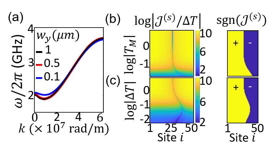
Figure 2: (a) The magnon dispersion of a wire with different widths $w_{y}$. The wavenumber $k$ corresponds to the peak of the Fourier transform of the spatial wave function. (b) and (c) Spin Seebeck current as a function of average temperature $T_{M}=(T_{L}+T_{R})/2$ and temperature difference $\Delta T=T_{R}-T_{L}$, respectively. Left: $|\mathcal{J}^{(s)}/\Delta T|$. Right: $\mathcal{J}^{(s)}/|\mathcal{J}^{(s)}|$. In (b), $\Delta T=10\,$mK. In (c), $T_{L}=20\,$mK. In (b) and (c), $w_{y}=500\,$nm [red curve in (a)]. In (a)-(c), $h^{z}=20\,$mT.

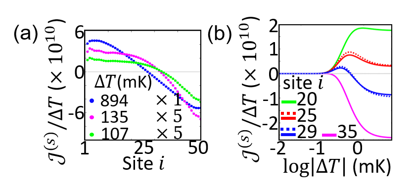
Figure 3: (a) Site dependence of $\mathcal{J}_{i}^{(s)}$ for the $\Delta T$ $=107,135,894\,$mK from Fig. 2(c). (b) Dependence of spin current $\mathcal{J}_{i}^{(s)}\left(\Delta T\right)$ of four sites $i$ on $\Delta T$, from Fig. 2(c). The dashed lines correspond to a finer mesh $d=25\,$nm (rather than 50 nm), illustrating convergence. In (a) and (b), $T_{L}=20\,$mK.

Temperature dependence - We apply a linear temperature gradient with $\Delta T=T_{R}-T_{L}$, $T_{L}$ ($T_{R}$) is the temperature at the left (right) edge of the nanowire. In linear response, the TSSE signal is antisymmetric, changing sign in the middle of the wire [4, 5, 26, 25, 24]. Figures 2(b) and (c) show amplitudes (left panels) and signs (right panels) of $\mathcal{J}_{i}^{s}/\Delta T$ as a function of $T_{M}=\left(T_{R}+T_{L}\right)/2$ and temperature difference $\Delta T$, respectively, for $w_{y}=500\,$nm and $h^{z}=20\,$mT [with dispersion in Fig. 2(a)]. In Fig. 2(b), we show the dependence on the mean temperature $T_{M}$ for fixed $\Delta T=10\,$mK. In Fig. 2(c), $T_{L}=20\,$mK is fixed and the gradient $\Delta T$ is varied. According to Figure 2(b), the signal increases with increasing $T_{M}$. The early saturation is an artifact by the frequency cut-off, $\omega_{\mathrm{max}}$, introduced by the finite mesh size $d$, so results are valid for $T<\hbar\omega_{\mathrm{max}}/k_{B}$. The qualitative features nevertheless remain intact for half the mesh size $d$, i.e. a $\sim 4$ times larger cutoff frequency, as illustrated in Fig. 3(b). The site index $i_{\pm}$ at which $\mathcal{J}_{i}^{s}$ changes sign in Fig. 2(b) shifts to the right edge with decreasing $T_{M}$ below $\hbar\omega_{c}/k_{B}=0.1\,$K, where $\omega_{c}$ is the uniform (Kittel) mode frequency. According to Fig. 2(c), the asymmetry survives at higher temperatures with increasing temperature difference $\Delta T$ and fixed $T_{L}\ll\hbar\omega_{c}/k_{B}$. Figures 3(a)-(b) emphasize the essence of the results in Fig. 2(c) (see also Fig. S1 [50]). Figure 3(a) shows the deviation of the signal from an antisymmetric profile. In Fig. 3(b), we observe that for a contact on the right half of the nanowire and fixed small $T_{L}=20\,$mK, the TSSE signal changes sign and a maximum appears at relatively large $\Delta T$ and $T_{M}$. The dashed curves in Fig. 3(b) show that for smaller mesh size $d$, i.e. higher cutoff frequency, the peak and sign change features remain intact. In the blue curves of Fig. 3(b), the $\Delta T^{\prime}$s that cause the sign change and peak are $\sim 0.4\,$K and $\sim 0.2\,$K, respectively.

The deviation from an antisymmetric signal can partly be understood in a semiclassical picture. The additional occupation of a magnon mode with frequency $\omega_{0}$ scales like $\delta n_{BE}\sim\tau_{r}v(\omega_{0})\nabla n_{BE}(\omega_{0})$ [12], where $\tau_{r}$ is a relaxation time, $v({\omega_{0}})$ is the group velocity, and $n_{BE}(\omega_{0})=\left(e^{\hbar\omega_{0}/k_{B}T}-1\right)^{-1}$. $\int_{\omega}\delta n_{BE}\neq 0$ because the magnons pile up or get drained at the edges. In linear response and a long spin-diffusion length the dependence is linear with a zero in the center. An expansion in $\hbar\omega_{0}/\left(k_{B}T\right)$ can only indicate that $\nabla n_{BE}(\omega_{0})$ is uniform for $T_{M}>\hbar\omega_{0}/k_{B}$ when $\Delta T\ll T_{M}$ [see Fig. 2(b)], and for $\Delta T\gg\hbar\omega_{0}/k_{B}$ when $T_{M}\sim\Delta T/2$ [see Fig. 2(c)]. A detailed calculation is indeed necessary to determine the spatial dependence of magnon accumulation in the nonlinear regime of temperature, where we observe a substantial non-monotonicity of signal at certain contact positions [see Fig. 3(b)].

The TSSE voltage $V_{i}^{(TSSE)}=2\rho\theta_{H}ew_{y}g_{r}\mathcal{J}_{i}^{s}/\left(4\pi w_{y}d\right)$, where $-e$ is the electron charge, and for Pt, the conductivity $\rho=0.9\,\mathrm{\mu{\Omega}\,}$m [46], spin Hall angle $\theta_{H}=0.07$ [45], while for the YIG/Pt interface $g_{r}/\left(w_{y}d\right)=10^{16}\,1/\text{m}^{2}$ [46]. This leads to $V_{i}^{(TSSE)}\approx 8\times 10^{-18}\mathcal{J}_{i}^{s}\,$V. The low temperature maximum of $\mathcal{J}_{i}^{s}/\Delta T\sim 10^{10}$ for $\Delta T=0.2\,$K [see Fig. 3(b)] leads to a substantial $V_{i}^{(TSSE)}\sim 16\,$nV.

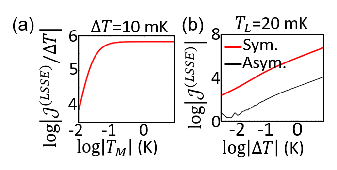
Figure 4: Longitudinal spin Seebeck effect. The temperature dependence of the spin current at the right endpoint flowing into a spin sink (a) $\Delta T=10\,$mK. (b) $T_{L}=20\,$mK. Here we plot $(\mathcal{J}_{L}^{(LSSE)}-\mathcal{J}_{R}^{(LSSE)})/2$ (red line labeled Sym) and $\mathcal{J}_{R}^{(LSSE)}+\mathcal{J}_{L}^{(LSSE)}$ (black line labeled Asym.)

LSSE - The LSSE records the total spin current generated in the magnet within the spin relaxation length and not just the magnon accumulation at the contact as in the TSSE. We can access the LSSE by modifying the boundary conditions at the terminals of the wire in order to allow the spin currents to flow unimpeded into the contacts that act as spin and energy sinks. To this end, we introduce two reservoirs to the left and right of the nanowire. We assume the reservoirs to be non-magnetic metals (NM) with a large spin mixing conductance and interfacial damping at both ends as detailed in [50]. This is in contrast to the contacts in the TSSE, which we assumed to be non-invasive. Figures 4(a) and (b) show temperature dependence of the average current through the wire $\mathcal{J}^{(LSSE)}=\left(\mathcal{J}_{R}^{(LSSE)}-\mathcal{J}_{L}^{(LSSE)}\right)/2$.  The temperature combinations of Figs. 4(a) and (b) are the same as in Figs. 2(a) and (b), i.e. fixed $\Delta T=10\,$mK but varying $T_{M}$ or fixed $T_{L}=20\,$mK but varying $\Delta T$, respectively. Figures 4(a) and (b) are featureless and illustrate that even for low $T_{M}\ll\Delta T$, $\mathcal{J}^{(LSSE)}$ depends (quasi-)linearly on $\Delta T$ [see Fig. 4(b)]. In Fig. 4(b), we also show difference of the spin currents into the left and out of the right contacts $\mathcal{J}_{R}^{(LSSE)}+\mathcal{J}_{L}^{(LSSE)}$, which turns out to be relatively very small because LSSE is dominated by the bulk spin current which is the same for both contacts. It should be emphasized that our TLS model is strictly valid only for $T<1\,$K.

Conclusion - We investigate SSE at cryogenic temperatures $T\lesssim 1\,$K with dissipation by two-level systems. In the nonlinear temperature regime, i.e. large $\Delta T/T$, we predict a non-monotonic TSSE signal at certain position of the detector contacts. For a linear temperature gradient, and a contact position in the hot region, the sign changes and a substantially large $\sim 10\,$nV voltage peak emerges at $2T_{M}\approx\Delta T\sim 0.2\,$K. On the other hand, the LSSE signal follows a (quasi-)linear dependence on $\Delta T$, even when much larger than the average temperature.

Acknowledgments -We acknowledge support by JSPS KAKENHI Grants with Nos. 20H02609 and 19H006450.

References

- [1] K. Uchida, S. Takahashi, K. Harii, J. Ieda, W. Koshibae, K. Ando, S. Maekawa, and E. Saitoh, Nature 455, 778 (2008).
- [2] K. Uchida, J. Xiao, H. Adachi, J. Ohe, S. Takahashi, J. Ieda, T. Ota, Y. Kajiwara, H. Umezawa, H. Kawai, G. E. W. Bauer, S. Maekawa, and E. Saitoh, Nat. Mater. 9, 894 (2010).
- [3] C. M. Jaworski, J. Yang, S. Mack, D. D. Awschalom, J. P. Heremans, and R. C. Myers, Nature Mater. 9, 898 (2010).
- [4] J. Xiao, G. E. W. Bauer, K.-C. Uchida, E. Saitoh, and S. Maekawa, Phys. Rev. B 81, 214418 (2010).
- [5] H. Adachi, J.-I. Ohe, S. Takahashi, and S. Maekawa, Phys. Rev. B 83, 094410 (2011).
- [6] G. E. W. Bauer, E. Saitoh, and B. J. van Wees, Nat. Mater. 11, 391 (2012).
- [7] Y. Ohnuma, H. Adachi, E. Saitoh, and S. Maekawa, Phys. Rev. B 87, 014423 (2013). 014416 (2014).
- [8] S. M. Wu, J. E. Pearson, and A. Bhattacharya, Phys. Rev. Lett. 114, 186602 (2015).
- [9] S. M. Wu, W. Zhang, A. KC, P. Borisov, J. E. Pearson, J. S. Jiang, D. Lederman, A. Hoffmann, and A. Bhattacharya, Phys. Rev. Lett. 116, 097204 (2016).
- [10] K. Uchida, H. Adachi, T. Ota, H. Nakayama, S. Maekawa, and E. Saitoh, Appl. Phys. Lett. 97, 172505 (2010)
- [11] L. J. Cornelissen, J. Liu, R. A. Duine, J. Ben Youssef, annd B. J. van Wees, Nat. Phys. 11, 1022 (2015).
- [12] S. M. Rezende, R. L. Rodriguez-Suarez, R. O. Cunha, A. R. Rodrigues, F. L. A. Machado, G. A. F. Guerra, J. C. L. Ortiz, and A. Azevedo, Phys. Rev. B 89, 014416 (2014).
- [13] T. Kikkawa, K.-I. Uchida, S. Daimon, Z. Qiu, Y. Shiomi, and E. Saitoh, Phys. Rev. B 92, 064413 (2015).
- [14] H. Jin, S. R. Boona, Z. Yang, R. C. Myers, and J. P. Heremans, Phys. Rev. B 92, 054436 (2015).
- [15] E.-J. Guo, J. Cramer, A. Kehlberger, C. A. Ferguson, D. A. MacLaren, G. Jakob, and M. Klaui, Phys. Rev. X 6, 031012 (2016).
- [16] M. Schreier, F. Kramer, H. Huebl, S. Geprags, R. Gross, and S. T. B. Goennenwein, Phys. Rev. B 93, 224430 (2016).
- [17] Ryo Iguchi, K.-I. Uchida, S. Daimon, and E. Saitoh, Phys. Rev. B 95, 174401 (2017).
- [18] A. De, A. Ghosh, R. Mandal, S. Ogale, and S. Nair, Phys. Rev. Lett. 124, 017203 (2020).
- [19] K. Oyanagi , T. Kikkawa , and E. Saitoh, AIP Advances 10, 015031 (2020).
- [20] K. Ganzhorn, T. Wimmer , J. Cramer, R. Schlitz, S. Geprägs, G. Jakob, R. Gross , H. Huebl, M. Kläui, and S. T. B. Goennenwein, AIP Advances 7, 085102 (2020).
- [21] L. Onsager, Phys. Rev. 37 405 (1931).
- [22] L. J. Cornelissen, K. J. H. Peters, G. E. W. Bauer, R. A. Duine, and B. J. van Wees, Phys. Rev. B 94, 014412 (2016).
- [23] K. Miyazakia and K. Seki, J. Chem. Phys. 108, 7052 (1998).
- [24] P. Yan, G. E. W. Bauer, and H. Zhang, Phys. Rev. B 95, 024417 (2017).
- [25] U. Ritzmann, D. Hinzke, A. Kehlberger, E.-J. Guo, M. Klaui, and U. Nowak, Phys. Rev. B 92, 174411 (2015).
- [26] J.-I. Ohe, H. Adachi, S. Takahashi, and S. Maekawa, Phys. Rev. B 83, 115118 (2011).
- [27] L. Chotorlishvili, Z. Toklikishvili, V. K. Dugaev, J. Barnas, S. Trimper, and J. Berakdar, Phys. Rev. B 88, 144429 (2013).
- [28] J. Barker and G. E. W. Bauer, Phys. Rev. Lett. 117, 217201 (2016).
- [29] J. Barker and G. E. W. Bauer, Phys. Rev. B 100, 140401 (2019).
- [30] T. Kikkawa, K. Shen, B. Flebus, R. A. Duine, K. Uchida, Z. Qiu, G. E. W. Bauer, and E. Saitoh, Phys. Rev. Lett. 117, 207203 (2016).
- [31] R. Schmidt and P. W. Brouwer, arXiv:2010.09571v1 (2020).
- [32] Y. Tabuchi, S. Ishino, T. Ishikawa, R. Yamazaki, K. Usami, and Y. Nakamura, Phys. Rev. Lett. 113, 083603 (2014).
- [33] J. H. Van Vleck, J. Appl. Phys. 35, 882 (1964).
- [34] E. G. Spencer, R. C. Lecraw, and R. C. Linarks Jr., Phys. Rev. 123, 1937 (1961).
- [35] J. H. Van Vleck and R. Orbach, Phys. Rev. Lett. 11, 65 (1963).
- [36] G. Schmidt, C. Hauser, P. Trempler, M. Paleschke, E. Th. Papaioannou, Phys. Status Solidi B 2020, 1900644 (2020).
- [37] Q. Wang, B. Heinz, R. Verba, M. Kewenig, P. Pirro, M. Schneider, T. Meyer, B. Lagel, C. Dubs, T. Bracher, and A. V. Chumak, Phys. Rev. Lett. 122, 247202 (2019).
- [38] D. D. Stancil and A. Prabhakar, Spin Waves (Springer, New York, 2009)
- [39] M. Elyasi, Y. M. Blanter, G. E. W. Bauer, Phys. Rev. B 101, 054402 (2020).
- [40] B. A. Kalinikos and A. N. Slavin, J. Phys. C: Solid State Phys. 19, 7013 (1986).
- [41] M. J. Hurben and C. E. Patton, J. Magn. Magn. Mater. 139, 263 (1995).
- [42] H. J. Carmichael, Statistical Methods in Quantum Optics, Springer (1999).
- [43] Y. Tserkovnyak, A. Brataas, G. E. W. Bauer, Phys. Rev. Lett. 88, 117601 (2002).
- [44] S. Zhang, Z. Li, Phys. Rev. Lett. 93, 127204 (2004).
- [45] L. Liu, T. Moriyama, D. C. Ralph, and R. A. Buhrman, Phys. Rev. Lett. 106, 036601 (2011).
- [46] Y. Kajiwara, K. Harii, S. Takahashi, J. Ohe, K. Uchida, M. Mizuguchi, H. Umezawa, H. Kawai, K. Ando, K. Takanashi, S. Maekawa, and E. Saitoh, Nature 464, 262 (2010).
- [47] A. J. Leggett, S. Chakravarty, A. T. Dorsey, M. P. A. Fisher, A. Garg, and W. Zwerger, Rev. Mod. Phys. (1987).
- [48] T. Prosen, J. Stat. Mech., P07020 (2010).
- [49] S. Ajisaka, F. Barra, C. Mejia-Monasterio, T. Prosen, Phys. Rev. B 86, 125111 (2012).
- [50] See supporting material for a TSSE temperature dependence example, the effect of dispersion monotonicity on TSSE, and for the model and calculation method of LSSE.