Hydrodynamics of particle systems with selection
via uniqueness for free boundary problems

Abstract.

We study an injection-branching-selection particle system on ${\mathbb{R}}$ at the hydrodynamic limit under arbitrarily varying injection and removal rates, where the corresponding free boundary problem (FBP) is not in general known to be solvable in the classical sense. We propose a weak formulation that does not involve the notion of a free boundary, but reduces to a FBP when classical solutions exist. It is based on second order parabolic equations with measure-valued right-hand side in conjunction with a complementarity condition. We show that the weak formulation characterizes the limit. We also study a branching-selection model of motionless particles with nonlocal branching in ${\mathbb{R}}^{d}$ under a general fitness function. The corresponding integro-differential FBP, shown to characterize the hydrodynamic limit, is an (irreducible) multi-dimensional evolution equation. In both results the treatment is based on FBP uniqueness.

1. Introduction

1.1. Background and motivation

In particle systems with spatial selection, particles living in ${\mathbb{R}}$ undergo motion, branching or injection, and selection. The last term refers to keeping the population size constant by removing, upon appearance of a new particle, the leftmost particle in the configuration. The first such systems were proposed in [7, 8] as models for natural selection in the evolution of a population, where the position of a particle represents the degree of fitness of an individual to its environment. A series of papers culminating in the monograph [11] studied a variety of related models motivated by particles interacting topologically (since, in the macroscopic version of the model, removals occur at the boundary of the configuration) and by particle systems in contact with current reservoirs. At the hydrodynamic limit (HDL) these models give rise to free boundary problems (FBP). Rigorously establishing the HDL–FBP relation requires control over regularity of the free boundary (such as $C^{1}$ or sometimes $C$). We are motivated by questions of characterizing HDL by PDE in cases where existing techniques might fall short of yielding free boundary regularity as well as when the FBP may not be solvable. This may happen, in particular, when the constant population size assumption is dropped and injection and removal rates vary at the macroscopic scale. The first goal of this paper is to introduce a weak formulation of FBP that does not involve the notion of a free boundary, and at the same time reduces to a classical FBP when classical solutions exist.

To put these questions in context, consider the $N$-particle Branching Brownian motion ($N$-BBM) in dimension 1, first studied in [26], which consists of $N$ particles performing Brownian motion (BM) independently, each branching into two at rate $1$. When branching occurs, the leftmost particle in the configuration is removed. The initial particle positions are drawn independently according to a probability measure $\xi_{0}$. Let $\xi^{N}_{t}=\sum_{i}\bdel_{X_{i}(t)}$ denote the configuration measure at time $t$, where $X_{i}(t)$ are the locations of the $N$ particles alive at time $t$. Here and throughout, $\bdel_{x}$ denotes the Dirac measure at $x$. Throughout, the bar notation will stand for normalization by $N$; in particular, $\bar{\xi}^{N}_{t}=N^{-1}\xi^{N}_{t}$. The corresponding FBP is to find a pair $(u,\ell)$, $\ell\in C(0,\infty):{\mathbb{R}})$, $u\in C({\mathbb{R}}\times(0,\infty):[0,\infty))\cap C^{2,1}(\{(x,t):t>0,x>\ell_{t}\})$ such that

(1.1) $$\begin{cases}\partial_{t}u-\frac{1}{2}\partial_{x}^{2}u=u&x>\ell_{t},\\ u=0&x\leq\ell_{t},\\ u(x,t)dx\to\xi_{0}(dx)&\text{weakly as }t\downarrow 0,\\ \int_{\mathbb{R}}u(x,t)dx=1.\end{cases}$$

It was shown in [14] (for $\xi_{0}$ possessing a density) that the process $\bar{\xi}^{N}_{t}$ has a deterministic limit, characterized in terms of barriers (see §3). Under the assumption that (1.1) has a classical solution and that the free boundary $\ell$ is $C^{1}$, it was further shown that the limit process has a density given by the unique solution to (1.1). In [4] is was then shown, for general $\xi_{0}$, that (1.1) has a unique classical solution and that the limit of $\bar{\xi}^{N}$ has a density given by $u$ (with $\ell$ only in $C$). In [11], a model we will refer to as the injection-selection model was studied, in which a collection of $N$ Brownian particles living in ${\mathbb{R}}_{+}$ and reflecting at the origin, is subject to injection of new particles at the origin, at times determined by a rate-$jN$ exponential clock, $j>0$ a constant. Upon each injection, the rightmost particle is removed. The corresponding FBP is to find $(u,\ell)$ such that

(1.2) $$\begin{cases}\partial_{t}u-\frac{1}{2}\partial^{2}_{x}u=0&0<x<\ell_{t},\\ u=0&x\geq\ell_{t},\\ -\frac{1}{2}\partial_{x}u(0,t)=-\frac{1}{2}\partial_{x}u(\ell_{t},t)=j,\\ u(\cdot,t)=u_{0},\end{cases}$$

with $u_{0}$ an initial density. It is shown there that the HDL exists and possesses a density. Moreover, to overcome questions of regularity of the free boundary, a weak formulation of solutions to (1.2) is proposed there, defined via approximations by local classical solutions, and it is proved that such a solution uniquely exists and is equal to the aforementioned HDL density (see §1.4 for more details).

The context in which our weak formulation is presented, in §1.2 below, is an injection-branching-selection particle system, which extends both the aforementioned ones. In this model, the mass conservation condition is abandoned, and the rates of injection and removal of mass may vary arbitrarily. As explained in Remark 2.7, such a perturbation has dramatic consequences on the macroscopic model to the extent that they may lead to high degree of irregularity of the free boundary, when a free boundary exists at all as a trajectory. It is not clear whether the current toolboxes of either the classical solution approach of [4] or the weak solution approach of [11] can potentially cover such scenarios. We will show that the weak formulation introduced here does.

Our second goal has to do with the applicability of what is sometimes called the ‘traditional’ approach to studying HDL, which consists of showing that limit laws are supported on solutions to a PDE that possesses a unique solution. In this paper we will refer to this as the uniqueness approach. The use of this approach has been missing from the literature on the subject; we refer to [13] for a discussion of the difficulty to apply it when the PDE is a FBP. We will show that the weak formulation fills this gap at least insofar as the injection-branching-selection model is concerned. (Below, we shall moreover apply the uniqueness approach to another model via a different toolbox.)

1.2. Injection-branching-selection and weak formulation

A brief description of the model is as follows. Brownian particles on the line, whose initial number is $N$, branch at rate $\kappa\geq 0$. In addition, injections occur according to a given point process, and removals occur at the left edge, with their number up to time $t$ given by a process $J^{N}_{t}$. The space-time injection and removal locations are denoted by ${\rm INJ}^{N}_{i}$ and ${\rm REM}_{i}^{N}$, $i\in{\mathbb{N}}$, respectively, and are encoded in random measures on ${\mathbb{R}}\times{\mathbb{R}}_{+}$, namely

(1.3) $$\alpha^{N}(dx,dt)=\sum_{i\in{\mathbb{N}}}\bdel_{{\rm INJ}^{N}_{i}}(dx,dt),\qquad\beta^{N}(dx,dt)=\sum_{i\in{\mathbb{N}}}\bdel_{{\rm REM}^{N}_{i}}(dx,dt).$$

As before, $\xi^{N}$ denotes the configuration process. Our scaling assumption is that one has $(\bar{\xi}^{N}_{0},\bar{\alpha}^{N},\bar{J}^{n})\to(\xi_{0},\alpha,J)$ in probability, where the latter is a deterministic tuple, and $J$ is absolutely continuous, nondecreasing and null at zero.

We can now provide a formal derivation of a PDE formulation that does not involve a free boundary. The fact that particles are always removed from the left side of the configuration can be expressed as a condition on $(\bar{\xi}^{N},\bar{\beta}^{N})$, namely

(1.4) $$\bar{\beta}^{N}(\{(x,t)\in{\mathbb{R}}\times{\mathbb{R}}_{+}:\bar{\xi}^{N}_{t}(-\infty,x)>0\})=0.$$

A key point is that $\bar{\beta}^{N}$ plays an additional role in the model, namely it drives the dynamics. Let us assume that in some sense $(\bar{\xi}^{N},\bar{\alpha}^{N},\bar{\beta}^{N})\to(\xi,\alpha,\beta)$ as $N\to\infty$, and moreover, that $\xi_{t}$ has a density $u(\cdot,t)$. Then the macroscopic dynamics should satisfy

$$\partial_{t}u-\frac{1}{2}\partial_{x}^{2}u-\kappa u=\alpha-\beta.$$

The precise definition of solutions to a second order parabolic equation with measure-valued RHS is given in §2. In this setting, the specification of $\xi_{0}$ as an initial condition of the dynamics can be achieved by adding the term $\xi_{0}\otimes\bdel_{0}$ to the RHS. Thus one is led to the following problem formulation. Let data $(\xi_{0},\alpha,J)$ be given. Denote $I_{t}=\alpha({\mathbb{R}}\times[0,t])$. Assume that the macroscopic total mass remains positive, namely that if $m_{t}=1+\kappa\int_{0}^{t}m_{s}ds+I_{t}-J_{t}$ then $m_{t}>0$ for all $t$. Find $(u,\beta)$, $u$ nonnegative, such that

(1.5) $$\begin{cases}\displaystyle\partial_{t}u-\frac{1}{2}\partial_{x}^{2}u-\kappa u=\alpha-\beta+\xi_{0}\otimes\bdel_{0}\\ \displaystyle\beta(U>0)=0\qquad\text{where}\qquad U(x,t)=\int_{-\infty}^{x}u(y,t)dy\\ \beta({\mathbb{R}}\times[0,t])=J_{t}.\end{cases}$$

For precise details see §2.2. We will refer to this as the weak FBP formulation, and to the condition $\beta(U>0)=0$ as the complementarity condition.

Our first main result, Theorem 2.4, states that, under mild assumptions on $\alpha$ and $J$, there exists a unique solution $(u,\beta)$ to (1.5), and, moreover, $(\bar{\xi}^{N},\bar{\beta}^{N})\to(\xi,\beta)$ in probability, where $\xi_{t}(dx)=u(x,t)dx$. The result is stated in a broader set up in which the particles follow a diffusion process on the line.

To recapitulate, this formulation circumvents the non-trivial obstacle of determining conditions for existence of a free boundary as a trajectory and related convergence issues, and, moreover, makes it possible to argue via PDE uniqueness.

1.3. Durrett-Remenik systems in ${\mathbb{R}}^{d}$

The $N$-BBM model has also been studied in ${\mathbb{R}}^{d}$, $d\geq 2$, where the removals are dictated by a given fitness function $F:{\mathbb{R}}^{d}\to{\mathbb{R}}$. Upon each branching, the particle whose $F$-value is smallest at the time is removed. The first paper to study this model was [5], where $F(x)=\|x\|$ and $F(x)=\lambda\cdot x$ were considered. As for results on HDL, the recent papers [2, 3] studied this model with $F(x)=-\|x\|$, corresponding to removal of the farthest particle from the origin in Euclidean metric, a model referred to as Brownian bees. The paper [2] studied the corresponding FBP showing existence and uniqueness, while [3] showed that the HDL is given as the unique classical solution to this FBP and provided estimates on rates of convergence. This treatment uses in a crucial way the symmetry of $F$, by which the radial projection of the macroscopic dynamics is governed by an autonomous equation, and in particular the motion of the free boundary is dictated by an equation in one dimension.

This motivates our third goal, namely to study a particle system in ${\mathbb{R}}^{d}$ with a fitness function that does not possess any symmetry. We do that for an extension to ${\mathbb{R}}^{d}$ of the model introduced in [18], of motionless non-locally branching particles on ${\mathbb{R}}$. Working with a general $F$ makes it a truly multidimensional selection model in the sense that the free boundary is not governed by a FBP in one spatial dimension. (Since particles do not move, it may seem that there is no significance to the dimension, as the model can be embedded in ${\mathbb{R}}$, for example; however, the topological structure, such as the continuity of $F$, is of crucial importance for the treatment of the model.)

Consider then a system of $N$ motionless particles living in ${\mathbb{R}}^{d}$ that branch nonlocally, where a particle at location $y$ gives birth at rate 1, and the location $x$ of the newborn is distributed according to $\rho(y,x)dx$, $\rho(y,\cdot)$ being a probability density for each $y$. The number of particles is kept constant by removing, upon each branching, the particle with least $F$-value, with $F$ a given fitness function. For $d=1$ and $F(x)=x$, this model was introduced and studied in [18], establishing the HDL and characterizing it by an integro-differential FBP.

Under mild assumptions on $\rho$ and $F$, our second main result, Theorem 2.9, states that the HDL exists and is characterized in terms of the unique solution to a FBP. This is the problem of finding a pair $(u,\ell)$, where $\ell:{\mathbb{R}}_{+}\to{\mathbb{R}}$ is càdlàg and the function $u:{\mathbb{R}}^{d}\times{\mathbb{R}}_{+}\to{\mathbb{R}}_{+}$ is $C^{0,1}$ in $\{(x,t)\in{\mathbb{R}}\times{\mathbb{R}}_{+}:F(x)>\ell_{t}\}$ and bounded on ${\mathbb{R}}^{d}\times[0,T]$ for any $T$, and one has

(1.6) $$\begin{cases}\displaystyle\partial_{t}u(x,t)=\int_{{\mathbb{R}}^{d}}u(y,t)\rho(y,x)dy&\quad(x,t):F(x)>\ell_{t},\,t>0,\\ u(x,t)=0&\quad(x,t):F(x)\leq\ell_{t},\,t>0,\\ \displaystyle\int_{{\mathbb{R}}^{d}}u(x,t)dx=1,&\quad t>0,\\ u(\cdot,0)=u_{0},\,\ell_{0}=\lambda_{0}.\end{cases}$$

The treatment of this model shares with the previous one the theme of implementing the uniqueness approach. A further aspect of this contribution has to do with a gap found in the proof of uniqueness of FBP solutions in [18], as we mention in Remark 2.11. Our result fills in this gap and validates the uniqueness statement of [18] (via a different technique).

1.4. Related work

Particle systems with selection and related models. In addition to HDL, the papers [14, 11, 13, 18, 2], already mentioned, have studied the long time behavior of the particle system or of the FBP, and [3] has established moreover the interchange of the $N$ and the $t$ limits. Although we have not addressed the long time behavior in this paper, it is of interest to consider this aspect in the weak formulation context in future work.

The first paper to study HDL for a model closely related to branching-injection was [10], where particles perform random walks on $[0,N]\cap{\mathbb{Z}}$ rather than BM. A variant of the $N$-BBM, in which the branching is nonlocal, was studied in [15], where the HDL was proved to exist with explicit bounds on the rates. The characterization of the limit as the solution of a FBP was also proved conditionally on existence of a classical solution to the latter, but existence is not known in general. The model can be seen to extend [18], in that the latter model is obtained when motion is switched off. However, the FBP corresponding to the model studied in [15] does not, strictly speaking, reduce to that from [18] by merely removing the Laplacian term, as we explain in Remark 2.12(b). Recently, in [23], the HDL of a system of Brownian particles with selection was characterized via the inverse first-passage time problem.

There are formal and rigorous relations between FBP (1.1) and (1.2) and the Stefan FBP (see [11, 2]). The latter was obtained as limits of variants of the symmetric simple exclusion process (SSEP) in [24, 25], as well as the limit of interacting diffusions with rank-dependent drift in [9]. In [13], a SSEP with birth of the leftmost hole and death of the rightmost particle was considered, and convergence at the hydrodynamic scale was proved. A rigorous connection to a FBP, obtained formally, was left open.

On earlier weak formulations. Relaxed solutions to (1.2) were proposed in [11], defined as the limit of a sequence of classical solutions to the FBP with perturbed data. Each term in the sequence is the classical solution to a FBP with piecewise $C^{1}$ free boundary, in which the initial condition and the mass conservation hold up to an error, which vanishes in the limit. The existence of these classical solutions is proved based on local existence to the Stefan problem. To the best of out knowledge, this idea has been implemented only for the model studied in [11], in which injection and removals occur at a constant rate, and injection occurs at the origin, and moreover, this was not aimed as a tool for applying the uniqueness approach.

The paper [16] introduced a probabilistic reformulation of the Stefan FBP and used it to define solutions beyond singularities, known to occur in the supercooled case of the problem. While the FBP are related, this formulation does not directly apply to the ones considered here.

On the barrier method. To the best of our knowledge, the idea of barriers was introduced into the subject in [10] and [13] (for particle systems with topological interaction, and, respectively, SSEP with free boundaries). Deterministic barriers are discrete versions of FBP that bound below and above any HDL of the model of interest, and have only one separating element. Their stochastic counterparts are particle systems which can be coupled to the particle system of interest in such a way that analogous bounds hold a.s. The use of deterministic barriers to proving uniqueness of a relaxed solution to a FBP first appeared in [11]. Both stochastic and deterministic barriers have since been used in [14, 15], and one of the ingredients in the proof of uniqueness of classical FBP solutions in both [4, 2] is closely related to the use of deterministic barriers. In these references, the proof that barriers form bounds on the FBP solution rely crucially on probabilistic representations of the latter. This tool is missing from our treatment as we are not aware of extensions of such representations that would apply to (1.5). Consequently, both the form of the barriers (specifically, the lower ones), and the proof that they provide bounds, are based on different considerations.

1.5. Organization of the paper

In §2, the models are introduced and the main results are stated, starting with §2.1 where the injection-branching-selection model is constructed, the weak FBP formulation is defined, and the main result on the model, Theorem 2.4, is stated. In §2.2, the Durrett-Remenik model is presented along with the result regarding it, Theorem 2.9. The remaining sections provide the proofs. In §3, the barrier method is used to prove uniqueness of solutions to the weak formulation. In §4, the convergence is proved by showing precompactness and that limit laws are supported on FBP weak solutions, which along with the results of §3, yield the proof of Theorem 2.4. Finally, §5 contains the proof of Theorem 2.9.

1.6. Notation

For $N\in{\mathbb{N}}$, $[N]:=\{1,2,\ldots,N\}$. In ${\mathbb{R}}^{d}$, denote the Euclidean norm by $\|\cdot\|$ and let $\mathbb{B}_{r}(x)=\{y\in{\mathbb{R}}^{d}:\|y-x\|\leq r\}$. Denote by ${\mathcal{M}}({\mathbb{R}}^{d})$ the space of finite signed Borel measures on ${\mathbb{R}}^{d}$ endowed with the topology of weak convergence. Let ${\mathcal{M}}_{1}({\mathbb{R}}^{d})\subset{\mathcal{M}}_{+}({\mathbb{R}}^{d})\subset{\mathcal{M}}({\mathbb{R}}^{d})$ denote the subsets of probability and, respectively positive measures, and give them the inherited topologies. Denote ${\mathbb{R}}_{+}=[0,\infty)$ and let ${\mathcal{M}}_{\rm loc}({\mathbb{R}}^{d}\times{\mathbb{R}}_{+})$ be the space of signed Borel measures on ${\mathbb{R}}^{d}\times{\mathbb{R}}_{+}$ that are finite on ${\mathbb{R}}^{d}\times[0,T]$ for every $T$ and give it the topology of weak convergence on ${\mathbb{R}}^{d}\times[0,T]$ for every $T$. Similarly, let ${\mathcal{M}}_{+,\rm loc}({\mathbb{R}}^{d}\times{\mathbb{R}}_{+})\subset{\mathcal{M}}_{\rm loc}({\mathbb{R}}^{d}\times{\mathbb{R}}_{+})$ be the subspace of positive measures with inherited topology. For $X={\mathbb{R}}^{d}$ or ${\mathbb{R}}^{d}\times{\mathbb{R}}_{+}$, for $\mu\in{\mathcal{M}}_{+}(X)$, denote $|\mu|=\mu(X)$. For $\mu,\nu\in{\mathcal{M}}_{+}(X)$, write $\mu\sqsubset\nu$ if $\mu(A)\leq\nu(A)$ for all measurable $A\subset X$.

For $u,v\in{\mathcal{B}}({\mathbb{R}}^{d},{\mathbb{R}})$ (Borel measurable) and $\xi\in{\mathcal{M}}_{+}({\mathbb{R}}^{d})$, denote $\langle u,\xi\rangle=\int u\,d\xi$ and $(u,v)=\int uv\,dx$. For $\xi\in{\mathcal{M}}_{+}({\mathbb{R}})$, $u\in L_{1}({\mathbb{R}})$ and an interval, say $[a,b]$, use $\xi[a,b]$ and $u[a,b]$ as shorthand for $\xi([a,b])$, and, respectively, $\int_{a}^{b}u\,dx$.

For $p\in[1,\infty]$, abbreviate $L_{p}({\mathbb{R}}^{d})$ to $L_{p}$, and for $u\in L_{p}$ denote $\|u\|_{p}=\|u\|_{L_{p}}$. Let $L_{p,\rm loc}({\mathbb{R}}_{+},L_{q})$ denote the linear space of functions from ${\mathbb{R}}_{+}$ to $L_{q}$ that are $p$-integrable on $[0,T]$ for every $T$.

For $(X,d_{X})$ a Polish space let $C({\mathbb{R}}_{+},X)$ and and $D({\mathbb{R}}_{+},X)$ denote the space of continuous and, respectively, càdlàg paths, endowed with the topology of uniform convergence on compacts and, respectively, the Skorohod $J_{1}$ topology. Let $C^{\uparrow}({\mathbb{R}}_{+},{\mathbb{R}}_{+})$ denote the subset of $C({\mathbb{R}}_{+},{\mathbb{R}}_{+})$ of nondecreasing functions that vanish at zero. For $I\in C^{\uparrow}({\mathbb{R}}_{+},{\mathbb{R}}_{+})$, denote by $dI_{t}$ the corresponding Stieltjes measure on ${\mathbb{R}}_{+}$. Denote by $AC^{\uparrow}({\mathbb{R}}_{+},{\mathbb{R}}_{+})$ the subset of $C^{\uparrow}({\mathbb{R}}_{+},{\mathbb{R}}_{+})$ of absolutely continuous functions. For $\rho\in(0,1]$ let $C^{\rho}({\mathbb{R}}_{+},{\mathbb{R}})$ denote the space of $\rho$-Hölder continuous functions starting at zero. Denote by $C_{c}^{\infty}(X)$ the space of compactly supported smooth functions on $X$ when $X={\mathbb{R}}^{d}$ or ${\mathbb{R}}^{d}\times{\mathbb{R}}_{+}$. For $f:{\mathbb{R}}_{+}\to X$ denote

$$w_{[T_{1},T_{2}]}(f,\delta)=\sup\{d_{X}(f(s),f(t)):T_{1}\leq s\leq t\leq(s+\delta)\wedge T_{2}\},$$

and $w_{T}=w_{[0,T]}$. For $(Y,|\cdot|)$ a normed space and $f:{\mathbb{R}}_{+}\to Y$, denote

$$\|f\|^{*}_{[T_{1},T_{2}]}=\sup\{|f(s)|:t\in[T_{1},T_{2}]\}\quad\text{and}\quad\|f\|^{*}_{T}=\|f\|^{*}_{[0,T]}.$$

The term with high probability (w.h.p.) means ‘away from an $N$-dependent event whose probability tends to zero as $N\to\infty$’. The symbol $c$ denotes a positive constant whose value may change from one expression to another.

2. Models and results

2.1. The injection-branching-selection model

2.1.1. Particle system construction

First we describe the motion that individual particles perform, namely a diffusion process with coefficients $\mathfrak{b}$ and $\mathfrak{c}$ satisfying

Assumption 2.1.

One has $\mathfrak{b}\in C^{1}({\mathbb{R}})$ and $\mathfrak{c}\in C^{2}({\mathbb{R}})$ with $\mathfrak{b}$, $\mathfrak{c}$ and its derivative $\mathfrak{c}^{\prime}$ bounded and $\mathfrak{c}$ bounded away from zero.

Given a one-dimensional BM $B$, denote by $\mathfrak{X}(x,s,B)$ the unique strong solution $\{X_{t}:t\in[s,\infty)\}$ to the SDE

(2.1) $$X_{t}=x+\int_{s}^{t}\mathfrak{b}(X_{\theta})d\theta+\int_{s}^{t}\mathfrak{c}(X_{\theta})dB_{\theta},\qquad t\in[s,\infty).$$

The particle system, defined on a probability space $(\mathnormal{\Omega},{\mathcal{F}},{\mathbb{P}})$, is indexed by $N$, where $N$ is the initial number of particles. The particles are indexed by the set ${\mathcal{S}}={\mathbb{N}}\times{\mathbb{Z}}_{+}$, where particles $i=(j,0)$ are roots of family trees, and particles $i=(j,k)$, $k\geq 1$ are descendants of $(j,0)$. Below, items (1)–(5) list stochastic primitives of the model, and (6) states a condition they satisfy.

1. A collection $\{x^{i}(N):i=(j,0),\ j\in[N]\}$ of real-valued random variables representing the initial positions of the particles in the initial configuration. For such $i$ set $\sigma^{i}(N)=0$, expressing the fact that these particles are introduced into the system at time $0$.

2. A collection $\{(x^{i}(N),\sigma^{i}(N)):i=(j,0),\ j=N+1,N+2,\ldots\}$ of ${\mathbb{R}}\times(0,\infty)$-valued random variables representing the initial space-time positions of injected particles, ordered by injection time, assumed distinct: $\sigma^{(N+1,0)}(N)<\sigma^{(N+2,0)}(N)<\cdots$.

3. A collection $\{B^{i}:i\in{\mathcal{S}}\}$ of mutually independent BM, driving the motion of the corresponding particles.

4. A collection $\{\pi^{i}:i\in{\mathcal{S}}\}$ of mutually independent rate-$\kappa$ Poisson processes, where $\kappa\geq 0$ is the branching rate, determining the times a living particle gives birth.

5. A sequence $0<\eta^{1}(N)<\eta^{2}(N)<\cdots$ of removal times.

6. The first four stochastic elements (1)–(4) are mutually independent.

The notation $x^{i}(N)$, $\sigma^{i}(N)$ and $\eta^{l}(N)$ is henceforth abbreviated to $x^{i}$, $\sigma^{i}$ and $\eta^{l}$.

The trajectories that particles follow are constructed in two steps. First, once the initial space-time position $(x^{i},\sigma^{i})$ of particle $i$ is determined, its potential trajectory, denoted $\{X^{i}_{t},t\in[\sigma^{i},\infty)\}$, is defined by

(2.2) $$X^{i}_{t}=\mathfrak{X}(x^{i},\sigma^{i},B^{i})(t),\qquad t\geq\sigma^{i}.$$

In the second step, the removal time $\tau^{i}$ of particle $i$ is determined (where $\infty$ is possible), and the actual trajectory the particle follows is obtained by trimming the potential trajectory at $\tau^{i}$.

The particle configuration is defined on $(\eta^{l},\eta^{l+1}]$ inductively for $l=0,1,\ldots$, where $\eta^{0}=0$. The configuration at time $0$ is given by $X^{i}_{0}=x^{i}$ for $i=(j,0)$, $j\in[N]$. This gives a well defined potential trajectory of each of these particles on $[0,\infty)$. Next, for $l\geq 0$, given the configuration during $[0,\eta^{l}]$, the construction during $(\eta^{l},\eta^{l+1}]$ is described as follows.

During the time interval $(\eta^{l},\eta^{l+1})$:

• Each of the particles living at $\eta^{l}$ already has a well defined potential trajectory. These particles live through the interval, with their actual trajectories given by their potential trajectories.

• Each $i$ of the form $(j,0)$ with $\sigma^{i}\in(\eta^{l},\eta^{l+1})$ corresponds to an injection during this interval. This determines the injection space-time location $(x^{i},\sigma^{i})$ of a new particle, and accordingly its potential trajectory for all $t\geq\sigma^{i}$. These particles live through the remainder interval.

• If a particle $i=(j,k)$ is alive when $\pi^{i}$ ticks, it gives birth to a new particle at that space-time location. The new particle gets the label $\hat{i}=(j,\hat{k}+1)$ where $(j,\hat{k})$ is the latest descendant of $(j,0)$ introduced prior to that time. Again, this determines the potential trajectory, and the particle lives through the remainder interval.

At the time $\eta^{l+1}$:

• If there are no particles in the system, nothing happens.

• If no new particle is introduced at that time then the particle that is leftmost at $\eta^{l+1}-$ is removed. If the index of this particle is $i$ then this determines its removal time as $\tau^{i}=\eta^{l+1}$.

• If a particle is introduced at $\eta^{l+1}$ (by injection or branching), the construction obeys the rule ‘introduce and then remove’, and this may cause the new particle to be removed immediately (i.e., if the injection is to the left of all particles or the branching particle is the leftmost).

By the independence assumptions, a.s., no simultaneous introduction of particles can occur after time $0$. For particles $i$ that never get removed, define $\tau^{i}=\infty$. The lifetime of particle $i$ is given by $[\sigma^{i},\tau^{i})$ (empty if $\sigma^{i}=\tau^{i}$ or $\sigma^{i}=\infty$) and its actual trajectory is defined by $\{X^{i}_{t}:\,t\in[\sigma^{i},\tau^{i})\}$. This completes the construction of the particle system.

Some useful notation is as follows. The set of particles initially in the system, injected and, respectively, descendants of a root particle $i=(j,0)$, are denoted by

$${\mathcal{S}}^{N,\rm init}=[N]\times\{0\},\qquad{\mathcal{S}}^{N,\rm inj}=\{N+1,N+2,\ldots\}\times\{0\},\qquad{\mathcal{S}}^{N,i}=\{(j,k):k\in{\mathbb{Z}}_{+}\}.$$

The set of particles introduced by time $t$ is

$${\mathcal{S}}^{N}_{t}=\{i\in{\mathcal{S}}:\sigma^{i}\leq t\}.$$

Those injected by time $t$ and, respectively, descendants of root particle $i$ introduced by time $t$, are denote by

(2.3) $${\mathcal{S}}^{N,\rm inj}_{t}={\mathcal{S}}^{N,\rm inj}\cap{\mathcal{S}}^{N}_{t},\qquad{\mathcal{S}}^{N,i}_{t}={\mathcal{S}}^{N,i}\cap{\mathcal{S}}^{N}_{t}.$$

Next, the configuration process is given by

$$\xi^{N}_{t}(dx)=\sum_{i\in{\mathcal{S}}}\bdel_{X^{i}_{t}}(dx)1_{\{\sigma^{i}\leq t<\tau^{i}\}},$$

and clearly its initial condition is

$$\xi_{0}^{N}(dx)=\sum_{i\in{\mathcal{S}}^{N,\rm init}}\bdel_{x^{i}}(dx).$$

The injection and, respectively, removal space-time locations are encoded by the random measures

(2.4) $$\alpha^{N}(dx,dt)=\sum_{i\in{\mathcal{S}}^{N,\rm inj}}\bdel_{(x^{i},\sigma^{i})}(dx,dt),\qquad\beta^{N}(dx,dt)=\sum_{i\in{\mathcal{S}}:\,\tau^{i}<\infty}\bdel_{(X^{i}_{\tau^{i}},\tau^{i})}(dx,dt).$$

Let $m^{N}_{t}=|\xi^{N}_{t}|$ denote the number of living particles at $t$. Let $I^{N}_{t}=\#{\mathcal{S}}^{N,\rm inj}_{t}$ be the number of injections by time $t$. Then $I^{N}_{t}=\alpha^{N}({\mathbb{R}}\times[0,t])$. Moreover, let $J^{N}_{t}=\#\{l\geq 1:\eta^{l}\leq t\}$ be the number of removal attempts by $t$. Note that the actual number of removals by $t$ is $\beta^{N}({\mathbb{R}}\times[0,t])$. Then $J^{N}_{t}=\beta^{N}({\mathbb{R}}\times[0,t])$ holds on the event $\{\inf_{s\leq t}m^{N}_{s}\geq 1\}$.

So far we have not made any assumption on the removal times $\eta^{l}$. We would like to cover the possibility that removals are synchronized with (some of the) injections or branching events, as well as that they occur independently of each other. Hence we let

(2.5) $${\mathcal{F}}^{N}_{t}=\sigma\{\xi^{N}_{0},\alpha^{N}(-\infty,x]\times[0,s],B^{i}_{s},\pi^{i}_{s},J^{N}_{s}:x\in{\mathbb{R}},s\in[0,t],i\in{\mathcal{S}}\},$$

and supplement (1)–(6) above with

• $B^{i}$ and $\hat{\pi}^{i}$ are $\{{\mathcal{F}}^{N}_{t}\}$-martingales, $i\in{\mathcal{S}}$, where $\hat{\pi}^{i}(t)=\pi^{i}(t)-\kappa t$.

2.1.2. Macroscopic problem data

The random elements just constructed, namely $\alpha^{N}$ and $\beta^{N}$ (respectively, $\xi^{N}_{0}$; $\xi^{N}$; $I^{N}$ and $J^{N}$) are viewed as random variables taking values in ${\mathcal{M}}_{+,{\rm loc}}({\mathbb{R}}\times{\mathbb{R}}_{+})$ (respectively, ${\mathcal{M}}_{1}({\mathbb{R}})$; $D({\mathbb{R}}_{+},{\mathcal{M}}_{+}({\mathbb{R}}))$; $D({\mathbb{R}}_{+},{\mathbb{R}})$). Our assumptions about the normalized data $(\bar{\xi}_{0}^{N},\bar{\alpha}^{N},\bar{J}^{N})$ are as follows.

Assumption 2.2.

As $N\to\infty$, $(\bar{\xi}^{N}_{0},\bar{\alpha}^{N},\bar{J}^{N})\to(\xi_{0},\alpha,J)$ in the product topology, in probability, where the latter is a deterministic tuple satisfying the following, for some $\rho_{0}>0$.

i. $\xi_{0}\in{\mathcal{M}}_{1}({\mathbb{R}})$, $\alpha\in{\mathcal{M}}_{+,\rm loc}({\mathbb{R}}\times{\mathbb{R}}_{+})$ and $J\in AC^{\uparrow}({\mathbb{R}}_{+},{\mathbb{R}}_{+})\cap C^{\rho_{0}}({\mathbb{R}}_{+},{\mathbb{R}}_{+})$.

ii. Denote $I_{t}=\alpha({\mathbb{R}}\times[0,t])$. Then one of the following holds:

• $\alpha(dx,dt)\sqsubset c\,dx\,dI_{t}$, some constant $c$. Moreover, $I\in C^{\uparrow}({\mathbb{R}}_{+},{\mathbb{R}}_{+})\cap C^{\rho_{0}}({\mathbb{R}}_{+},{\mathbb{R}}_{+})$.

• $I\in C^{\uparrow}({\mathbb{R}}_{+},{\mathbb{R}}_{+})\cap C^{\frac{1}{2}+\rho_{0}}({\mathbb{R}}_{+},{\mathbb{R}}_{+})$.

iii. Let $m$ denote the solution to

(2.6) $$m_{t}=1+\kappa\int_{0}^{t}m_{s}ds+I_{t}-J_{t},$$

representing the total macroscopic mass. Then $\varepsilon_{0}:=\inf_{t\in{\mathbb{R}}_{+}}m_{t}>0$.

A tuple $(\xi_{0},\alpha,J)$ satisfying conditions (i–iii) in Assumption 2.2 will be called an admissible macroscopic data.

Remark 2.3.

We can see that this setting extends the $N$-BBM to a BBM with variable removal rate. Namely, let the initial configuration be given by $N$ IID locations drawn from $\xi_{0}$. Let $J\in AC^{\uparrow}({\mathbb{R}}_{+},{\mathbb{R}}_{+})$ be given, and assume $m_{t}$ remains positive at all times, where

$$m_{t}=1+\int_{0}^{t}m_{s}ds-J_{t}.$$

Let $J^{N}$ be an inhomogeneous Poisson process with intensity function $NJ^{\prime}_{t}$. Then Assumption 2.2 is satisfied with $\alpha=0$, $\kappa=1$. The special case $J_{t}=t$, $(\mathfrak{b},\mathfrak{c})=(0,1)$ is precisely the $N$-BBM.

Similarly, the injection-selection model of [11], mentioned in the introduction, is closely related. In this model the injections and removals are coupled, which is allowed by our assumptions. Consider $\kappa=0$, $\alpha^{N}$ a Poisson point process with intensity $N\pi(dx)jdt$, where $\pi$ is any probability measure and $j>0$ a constant, and $J^{N}=I^{N}=\alpha^{N}({\mathbb{R}}\times[0,t])$. The case $\pi=\bdel_{0}$ gives the model from [11] except the minor point that the particles live in ${\mathbb{R}}$ rather than ${\mathbb{R}}_{+}$.

2.1.3. Weak FBP formulation and main result

First we recall the notion of second order parabolic equations with measure-valued RHS [1]. Let $\mathfrak{a}=\frac{1}{2}\mathfrak{c}^{2}$ and

(2.7) $${\mathcal{L}}\varphi=\mathfrak{a}\partial_{x}^{2}\varphi+\mathfrak{b}\partial_{x}\varphi+\kappa\varphi,\qquad{\mathcal{L}}^{*}u=\partial_{x}^{2}(\mathfrak{a}u)-\partial_{x}(\mathfrak{b}u)+\kappa u.$$

For $\mu\in{\mathcal{M}}_{\rm loc}({\mathbb{R}}\times{\mathbb{R}}_{+})$ consider the equation

(2.8) $$\partial_{t}u-{\mathcal{L}}^{*}u=\mu\qquad\text{ in }\qquad{\mathbb{R}}\times{\mathbb{R}}_{+}.$$

Let $q\in(1,\infty)$. A weak $L_{q}$-solution of (2.8) is a function $u\in L_{1,\rm loc}({\mathbb{R}}_{+},L_{q})$ satisfying

(2.9) $$-\int_{0}^{\infty}(\partial_{t}\varphi+{\mathcal{L}}\varphi,u)dt=\int_{{\mathbb{R}}\times{\mathbb{R}}_{+}}\varphi\,d\mu$$

for all $\varphi\in C_{c}^{\infty}({\mathbb{R}}\times{\mathbb{R}}_{+})$. In this paper we will always take $\mu$ to be of the form $\mu=\tilde{\mu}+\xi_{0}\otimes\bdel_{0}$, where $\tilde{\mu}$ does not charge ${\mathbb{R}}\times\{0\}$ and $\xi_{0}$ is a probability measure on ${\mathbb{R}}$. In this case the RHS above is given by

$$\int\varphi(\cdot,0)d\xi_{0}+\int_{{\mathbb{R}}\times{\mathbb{R}}_{+}}\varphi\,d\tilde{\mu},$$

showing that $\xi_{0}$ serves as an initial condition in the dynamics.

Such problems were analyzed in [1]. In particular, [1, Theorem 1 and Remark 1] show that for $1<q<\infty$, this problem possesses a unique weak $L_{q}$-solution, independent of $q$ (note that with the transformation $\bar{\mathfrak{a}}=\mathfrak{a}$, $\bar{\mathfrak{b}}=-\mathfrak{b}+\mathfrak{a}^{\prime}$, $\bar{\kappa}=\kappa-\mathfrak{b}^{\prime}$, one has the divergence form ${\mathcal{L}}^{*}u=\partial_{x}(\bar{\mathfrak{a}}\partial_{x}u)+\bar{\mathfrak{b}}\partial_{x}u+\bar{\kappa}u$, as required in [1, Remark 1(e)]). In what follows we thus use the term weak solution to (2.8), without reference to $q$.

We base on this notion the following problem formulation. Let admissible data $(\xi_{0},\alpha,J)$ be given. Consider the equation

(2.10) $$\begin{cases}{\it(i)}\hskip 35.00005pt\partial_{t}u-{\mathcal{L}}^{*}u=\alpha-\beta+\xi_{0}\otimes\bdel_{0}&\text{in }{\mathbb{R}}\times{\mathbb{R}}_{+},\\ {\it(ii)}\hskip 31.0001pt\beta(U>0)=0&\text{where}\qquad\displaystyle U(x,t)=\int_{-\infty}^{x}u(y,t)dy,\\ {\it(iii)}\hskip 27.0pt\beta({\mathbb{R}}\times[0,t])=J_{t}&\text{for }t\in{\mathbb{R}}_{+}.\end{cases}$$

A solution $(u,\beta)$ to (2.10) is defined as a member of $L_{1,\rm loc}({\mathbb{R}}_{+},L_{q})\times{\mathcal{M}}_{+,\rm loc}({\mathbb{R}}\times{\mathbb{R}}_{+})$ for some (equivalently, all) $q\in(1,\infty)$, such that $u$ is an a.e. non-negative weak solution to (2.10)(i), and moreover, conditions (2.10)(ii) and (2.10)(iii) hold.

Theorem 2.4.

Let Assumptions 2.1 and 2.2 hold. Then
i. There exists a unique solution $(u,\beta)$ to (2.10).
ii. There exists a version of $u$, again denoted $u$, such that setting $\xi_{t}(dx)=u(x,t)dx$ gives $\xi\in C({\mathbb{R}}_{+},{\mathcal{M}}_{+}({\mathbb{R}}))$, and $(\bar{\xi}^{N},\bar{\beta}^{N})\to(\xi,\beta)$ in probability as $N\to\infty$.

Remark 2.5.

The notion (2.10) can be seen as an extension of a classical solution to a FBP. For example, consider (1.2) and assume that $(u,\ell)$ is a classical solution, with $\ell\in C({\mathbb{R}}_{+},{\mathbb{R}})$ and $u$ appropriately smooth. Then a solution $(u,\beta)$ to (2.10) is obtained by $\beta(dx,dt)=\bdel_{\ell_{t}}(dx)jdt$, as can be verified directly.

Remark 2.6.

Some conclusions can be drawn from [1, Theorem 1] about regularity of solutions to (2.8), such as $u\in L_{p,\rm loc}({\mathbb{R}}_{+},W^{\sigma}_{q})$ for suitable values of $p$ and $\sigma$. These estimates will not be used here.

Remark 2.7.

Complex behavior of $I$ and $J$ can lead to higher and higher degree of free boundary irregularity. For example, consider the case ${\mathcal{L}}^{*}u=\partial_{x}^{2}u+u$, $\alpha=0$, a setting similar to (1.1) but with general $J$. If $J_{t}=|[0,t]\cap K|$, where $K=[0,1]\cup[2,\infty)$, then during the time interval $[0,1]$, there exists a classical solution to (1.1) with a continuous free boundary, by the results of [4]. During $[1,2]$ there is no absorption of mass, hence at time $1$, the free boundary jumps to $-\infty$ and stays there until time $2$; and during $(2,\infty)$ it is again finite and continuous. One can obtain this way countably many discontinuities on a finite time interval. Proceeding to a general Borel set $K$, it is plausible that classical solutions with a free boundary given as a trajectory will not in general exist. However, we are not aware of a rigorous result to that effect.

2.2. The Durrett-Remenik model

The particle model is as follows. The initial positions of particles are again denoted by $x^{i}$, $1\leq i\leq N$, which are now ${\mathbb{R}}^{d}$-valued RV. The number of particles remains $N$ at all times. An independent exponential clock of rate 1 is attached to each particle. When the clock of a particle rings, it gives birth to a new one. The location of a particle born from a particle at $x$ is drawn according to a probability density $\rho(x,\cdot)$ defined on ${\mathbb{R}}^{d}$. When a particle is born, the particle that has the least $F$-value among the living ones and the newborn, is removed, where the fitness function $F:{\mathbb{R}}^{d}\to{\mathbb{R}}$ is given. Ties are broken according to some fixed measurable total order on ${\mathbb{R}}^{d}$. As before, the configuration measure at time $t$ is denoted by $\xi^{N}_{t}$, and $\bar{\xi}^{N}_{t}=N^{-1}\xi^{N}_{t}$. In particular, the initial configuration is $\xi^{N}_{0}=\sum\bdel_{x^{i}}$.

Following is our assumption on $F$, $\rho$ and $\xi^{N}_{0}$. Denote $\ell^{N}_{0}=\min\{F(y):y\in{\rm supp}(\xi^{N}_{0})\}$.

Assumption 2.8.

(i) $F\in C({\mathbb{R}}^{d},{\mathbb{R}})$, $\inf_{x}F(x)=-\infty$, $\sup_{x}F(x)=\infty$, and for every $a\in{\mathbb{R}}$, $F^{-1}\{a\}$ has Lebesgue measure zero.

(ii) There exists a probability density $\tilde{\rho}$ and a constant $\tilde{c}$ such that $\rho(x,y)\leq\tilde{c}\tilde{\rho}(y-x)$. Moreover, $\rho(x,y)$ is continuous in $y$ uniformly in $(x,y)$, and for every $a\in{\mathbb{R}}$ and $x\in F^{-1}(a,\infty)$, one has $\int_{F^{-1}(a,\infty)}\rho(x,y)dy>0$.

(iii) As $N\to\infty$, $(\bar{\xi}^{N}_{0},\ell^{N}_{0})\to(\xi_{0},\lambda_{0})$ in probability, where the latter tuple is deterministic, $\xi_{0}(dx)=u_{0}(x)dx$ and $\lambda_{0}\in{\mathbb{R}}$. Moreover, $u_{0}$ is bounded and continuous on $F^{-1}(\lambda_{0},\infty)$ (and necessarily vanishes on $F^{-1}(-\infty,\lambda_{0})$), and for every $\delta>0$ and $\lambda\geq\lambda_{0}$, $\int_{F^{-1}(\lambda,\lambda+\delta)}u_{0}(x)dx>0$.

Further notation is $\ell^{N}_{t}=\min\{F(y):y\in{\rm supp}(\xi^{N}_{t})\}$ for the minimal $F$ value of all living particles at time $t$, and $J^{N}$ for the removal counting process.

We next write an equation for the macroscopic dynamics. Denote by ${\mathcal{X}}$ the set of pairs $(u,\ell)$, where $\ell\in D({\mathbb{R}}_{+},{\mathbb{R}})$ and the function $u:{\mathbb{R}}^{d}\times{\mathbb{R}}_{+}\to{\mathbb{R}}_{+}$ is $C^{0,1}$ in $\{(x,t)\in{\mathbb{R}}\times{\mathbb{R}}_{+}:F(x)>\ell_{t}\}$ and bounded on ${\mathbb{R}}^{d}\times[0,T]$ for any $T$. Consider the system

(2.11) $$\begin{cases}\displaystyle{\it(i)}\hskip 35.00005pt\partial_{t}u(x,t)=\int_{{\mathbb{R}}^{d}}u(y,t)\rho(y,x)dy&\quad(x,t):F(x)>\ell_{t},\,t>0,\\ {\it(ii)}\hskip 31.0001ptu(x,t)=0&\quad(x,t):F(x)\leq\ell_{t},\,t>0,\\ {\it(iii)}\hskip 25.00003pt\displaystyle\int_{{\mathbb{R}}^{d}}u(x,t)dx=1,&\quad t>0,\\ {\it(iv)}\hskip 28.99997ptu(\cdot,0)=u_{0},\,\ell_{0}=\lambda_{0}.\end{cases}$$

A solution to (2.11) is defined as a member of ${\mathcal{X}}$ satisfying (2.11).

Theorem 2.9.

Let Assumption 2.8 hold. Then there exists a unique solution to (2.11), denoted by $(u,\ell)$. Moreover, $\ell-\lambda_{0}\in C^{\uparrow}({\mathbb{R}}_{+},{\mathbb{R}})$. Furthermore, $(\bar{\xi}^{N},\ell^{N})\to(\xi,\ell)$, in probability, where $\xi_{t}(dx)=u(x,t)dx$.

Remark 2.10.

Because, as stated above, the $\ell$ component of any solution to (2.11) is nondecreasing, (2.11)(i) can be written in integral form as

$$u(x,t)=u_{0}(x)+\int_{0}^{t}\int_{{\mathbb{R}}^{d}}u(y,s)\rho(y,x)dydt,\qquad(x,t):F(x)>\ell_{t},t>0.$$

In a more general setting (not covered in this paper) where the mass conservation condition is dropped, $\ell$ need not be nondecreasing. In this case the system (2.11) is not sufficient for characterizing $(u,\ell)$. Roughly speaking, a boundary condition $u(\ell_{t},t)=0$ should be added at times when $\ell_{t}$ is decreasing. A precise way to write this is

$$u(x,t)=u_{0}(x)1_{\{\tau(t,x)=0\}}+\int_{\tau(t,x)}^{t}\int_{{\mathbb{R}}^{d}}u(y,s)\rho(y,x)dydt,\qquad(x,t):F(x)>\ell_{t},t>0,$$

where $\tau(x,t)=\inf\{s\in[0,t]:\ell_{\theta}<x\text{ for all }\theta\in(s,t)\}$.

Remark 2.11.

As explained in Remarks 1.1 and 2.10 of a recent version of [19], there appears to be a gap in the proof of [18, Theorem 1], specifically, the proof of uniqueness of solutions to the integro-differential free boundary problem, equation (FB) (corresponding to (2.11) above in the case $d=1$ and $F(x)=x$). Since convergence and uniqueness are proved in [18, Theorem 1] separately, this does not affect the validity of the convergence to a solution of (FB), as stated in that result, only the validity of the statement that the limit is uniquely characterized by this equation. We will recover the uniqueness statement by a different approach, in Lemma 5.2 below (and as a result, [18, Theorem 1] is fully valid).

Remark 2.12.

a. Theorem 2.9 goes beyond [18] even for $d=1$, as $F$ need not be monotone.
b. $N$-BBM with nonlocal branching was studied in [15], where particles perform BM on the line between branching events, and the limit was characterized by a FBP (in a form similar to (2.11)(i) above, with an additional Laplacian term), conditional on the existence of a classical solution with a $C^{1}$ free boundary. Although [15] extends the model from [18], the FBP from the former does not, strictly speaking, reduce to that from the latter by merely removing the Laplacian term, because a solution to the former, defined as a smooth function, must satisfy a Dirichlet condition at the free boundary, in contrast to solutions to the latter (or to (2.11)), which are typically discontinuous along the curve.

3. Injection-branching-selection: Uniqueness via barriers

In this section we prove the following result.

Theorem 3.1.

Let Assumption 2.1 hold and let admissible data $(\xi_{0},\alpha,J)$ be given. Then there exists at most one solution $(u,\beta)$ to (2.10).

The proof is based on the construction of barriers, which are shown to constitute upper and lower bounds to any solution, in the sense of mass transport inequalities. This section is structures as follows. Essential tools are developed in §3.1 and §3.2, where the former provides so called mild solutions, and the latter introduces operators required for the construction, and studies their properties in relation to mass transport inequalities. A sketch of the proof via barriers is given in §3.3. The upper and lower barriers are constructed in §3.4 and §3.5. In §3.6 it is shown that the barriers can be made close to each other, and the proof is completed.

3.1. Preliminary lemmas

The backward Kolmogorov equation associated with the diffusion (2.1) is given by $\partial_{t}u={\mathcal{L}}_{1}u$ with ${\mathcal{L}}_{1}u=\mathfrak{a}\partial_{x}^{2}u+\mathfrak{b}\partial_{x}u$. Denote by $\mathfrak{p}_{t}(x,y)$ the fundamental solution of this equation.

Lemma 3.2.

Given $T$ there exist constants $\tilde{c}_{1},\tilde{c}_{2},\hat{c}_{1},\hat{c}_{2}>0$ such that for $t\in(0,T]$ and $x,y\in{\mathbb{R}}$,

(3.1) $$\tilde{c}_{1}t^{-1/2}e^{-\tilde{c}_{2}(x-y)^{2}t^{-1}}\leq\mathfrak{p}_{t}(x,y)\leq\hat{c}_{1}t^{-1/2}e^{-\hat{c}_{2}(x-y)^{2}t^{-1}}.$$

Whereas the upper bound will be used many times, the lower bound is needed only to make the following statement (used in Lemma 3.8): There exists a constant $c_{*}>0$ such that

(3.2) $$\int_{-\infty}^{x}\mathfrak{p}_{t}(x,y)dy\geq c_{*},\qquad t\in(0,1],\,x\in{\mathbb{R}}.$$

Proof.

For $T=1$ these bounds follow from [27, Theorems 4.4.6 and 4.4.12]. To verify the assumptions, note that one can write ${\mathcal{L}}_{1}$ in the form ${\mathcal{L}}_{1}u=\partial_{x}(\mathfrak{a}\partial_{x}u)+\tilde{\mathfrak{b}}\mathfrak{a}\partial_{x}u$ by setting $\tilde{\mathfrak{b}}=(\mathfrak{b}-\mathfrak{a}^{\prime})\mathfrak{a}^{-1}$. The boundedness of $\tilde{\mathfrak{b}}$ follows from the assumed boundedness of $\mathfrak{a}^{-1}$, $\mathfrak{a}^{\prime}$ and $\mathfrak{b}$. For $T>1$, apply the scaling property of $\mathfrak{p}$ as in [27, Remark 4.1.5] (with constants depending on $T$). ∎

Denote

(3.3) $$\mathfrak{s}_{t}(x,y)=e^{\kappa t}\mathfrak{p}_{t}(x,y).$$

For $u\in L_{1}({\mathbb{R}})$ denote

(3.4) $$S_{t}u(y)=\int_{\mathbb{R}}\mathfrak{s}_{t}(x,y)u(x)dx,$$

and with a slight abuse of notation, use the same symbol for $\xi\in{\mathcal{M}}_{+}({\mathbb{R}})$, namely

(3.5) $$S_{t}\xi(y)=\int_{\mathbb{R}}\mathfrak{s}_{t}(x,y)\xi(dx).$$

For $\gamma\in{\mathcal{M}}_{+,{\rm loc}}({\mathbb{R}}\times{\mathbb{R}}_{+})$ and $0\leq\tau<t$, denote

$$S*\gamma(y,t)=\int_{{\mathbb{R}}\times[0,t]}\mathfrak{s}_{t-s}(x,y)\gamma(dx,ds),$$

$$S*\gamma(y,t;\tau)=\int_{{\mathbb{R}}\times[\tau,t]}\mathfrak{s}_{t-s}(x,y)\gamma(dx,ds).$$

Lemma 3.3.

i. Let $\gamma\in{\mathcal{M}}_{+,\rm loc}({\mathbb{R}}\times{\mathbb{R}}_{+})$ be such that $\gamma({\mathbb{R}}\times[0,\cdot])\in C^{\rho_{0}}({\mathbb{R}}_{+},{\mathbb{R}}_{+})$ for some $\rho_{0}>0$. Let $v(y,t)=S_{t}\xi_{0}(y)+S*\gamma(y,t)$. Then, for $q\in(1,\infty)$, $v\in L_{1,\rm loc}({\mathbb{R}}_{+},L_{q})$.

ii. Let $(\tilde{u},\beta)$ be a solution to (2.10). If $u$ is a version of $\tilde{u}$ then $(u,\beta)$ is also a solution. Moreover, $\tilde{u}$ has a version given by

(3.6) $$u(y,t)=S_{t}\xi_{0}(y)+S*\alpha(y,t)-S*\beta(y,t).$$

iii. One has $\|u(\cdot,t)\|_{1}=m_{t}$, $t>0$. Moreover, $\|v(\cdot,t)\|_{\infty}$ and $\|u(\cdot,t)\|_{\infty}$ are bounded locally for $t\in(0,\infty)$.

iv. One has, for $0<\tau<t$,

(3.7) $$u(y,t)=S_{t-\tau}u(\cdot,\tau)(y)+S*\alpha(y,t;\tau)-S*\beta(y,t;\tau).$$

Remark 3.4.

In what follows, by a solution to (2.10) we will mean the version given by (3.6) unless stated otherwise. In view of Lemma 3.3, there is no loss in doing so when proving the uniqueness result.

Proof.

i. Fix $T$. In this proof, $c$ denotes a constant not depending on $x,y$ and $t\in(0,T]$ whose value may change from one expression to another. By Lemma 3.2 and (3.3), it is easy to see that $\|\mathfrak{s}_{t}(x,\cdot)\|_{2}\leq ct^{-1/2}$, $t\in(0,T]$. By Minkowski’s integral inequality it follows that $\|S_{t}\xi_{0}\|_{2}\leq ct^{-1/2}$.

Next, let $q\in(1,\infty)$. Then by Lemma 3.2 and (3.3), for $t\in(0,T]$, $\|\mathfrak{s}_{t}(x,\cdot)\|_{q}\leq ct^{-Q}$ where $Q=(q-1)/(2q)$. By Minkowski’s integral inequality,

$$\|S*\gamma(\cdot,t)\|_{q}\leq c\int_{{\mathbb{R}}\times[0,t]}(t-s)^{-Q}\gamma(dx,ds)=c\int_{[0,t]}(t-s)^{-Q}dK_{s},$$

where $K_{t}=\gamma({\mathbb{R}}\times[0,t])$. By monotone convergence, the last integral is the limit as $\varepsilon\downarrow 0$ of

$$\int_{[0,t-\varepsilon]}(t-s)^{-Q}dK_{s} =K_{t-\varepsilon}\varepsilon^{-Q}-Q\int_{0}^{t-\varepsilon}K_{s}(t-s)^{-1-Q}ds$$

$$=(K_{t-\varepsilon}-K_{t})\varepsilon^{-Q}+Q\int_{0}^{t-\varepsilon}(K_{t}-K_{s})(t-s)^{-1-Q}ds+K_{t}t^{-Q}$$

(3.8) $$\leq c\int_{0}^{t}(t-s)^{\rho_{0}-1-Q}ds+K_{t}t^{-Q}.$$

If we choose $q>1$ sufficiently small then $\rho_{0}-1-Q\in(-1,0)$, and the above integral is bounded by $c$ for $t\leq T$. Moreover, $Q\in(0,1)$, and we obtain that $\|S*\gamma(\cdot,t)\|_{q}$ is integrable over $[0,T]$.

The two terms defining $v$ satisfy (2.9) for $\mu=\xi_{0}\otimes\bdel_{0}$ and $\gamma$, respectively, by a standard calculation which we omit. The estimates above on these two terms shows that they are, respectively, members of $L_{1,\rm loc}({\mathbb{R}}_{+},L_{2})$, and $L_{1,\rm loc}({\mathbb{R}}_{+},L_{q})$ for $q$ close to $1$. Hence each is a weak $L_{q}$-solution of the corresponding equation some $q\in(1,\infty)$. By the results of [1] discussed following (2.9), they must therefore be the unique weak $L_{q}$-solution, for all $q\in(1,\infty)$. This proves the assertion.

ii. For the first assertion we must show that the complementary condition (2.10)(ii) is preserved by changing $\tilde{u}$ to $u$. If $U$ is as in (2.10)(ii) and $\tilde{U}$ is defined similarly, then there is a set $A\subset{\mathbb{R}}_{+}$ of full Lebesgue measure such that $U(x,t)=\tilde{U}(x,t)$ for $(x,t)\in{\mathbb{R}}\times A$. Owing to the assumption that $J$ is absolutely continuous, $\beta$ does not charge ${\mathbb{R}}\times A^{c}$. This shows that $\beta(U>0)$ holds if and only if $\beta(\tilde{U}>0)$, proving the assertion.

For the second assertion, the arguments given above in (i) show that the three terms on the right of (3.6) are, for every $q\in(1,\infty)$, weak $L_{q}$-solutions of (2.8) for $\mu=\xi_{0}\otimes\bdel_{0}$, $\alpha$ and, respectively, $-\beta$. By linearity in $\mu$ of weak solutions of (2.8) [1, Theorem 1], it follows that $u$ defined in (3.6) is a weak $L_{q}$-solution of (2.10)(i) corresponding to data $(\xi_{0},\alpha,\beta)$. In particular, $u$ must be a version of $\tilde{u}$ by uniqueness of solutions to (2.8).

iii. To calculate $\tilde{m}_{t}:=\|u(\cdot,t)\|_{1}$, note that $\|\mathfrak{s}_{t}(x,\cdot)\|_{1}=e^{\kappa t}$. Hence by (3.6),

$$\tilde{m}_{t}=e^{\kappa t}+\int_{0}^{t}e^{\kappa(t-s)}dI_{s}-\int_{0}^{t}e^{\kappa(t-s)}dJ_{s},$$

which solves (2.6), and by uniqueness, equals $m_{t}$.

As for the estimate on $\|u(\cdot,t)\|_{\infty}$, by positivity we only need to estimate the first two terms in (3.6). Directly from Lemma 3.2, the sum of these two terms is bounded as follows:

$$\mathfrak{s}_{t}(x,y)\leq ct^{-1/2}+cI_{t}\qquad\text{and}\qquad ct^{-1/2}+c\int_{0}^{t}(t-s)^{-1/2}dI_{s},$$

under Assumption 2.2(ii.1) and, respectively, (ii.2). The former expression is locally bounded for $t$ away from $0$, as required. As for the latter, a calculation as in (3.8), replacing $(Q,\rho_{0},K_{t})$ by $(\frac{1}{2},\frac{1}{2}+\rho_{0},I_{t})$, shows that this expression is also locally bounded for $t$ away from $0$.

iv. Finally, (3.7) follows from (3.6) upon using the Chapman-Kolmogorov equation $\int\mathfrak{p}_{t-\tau}(x,y)\mathfrak{p}_{\tau}(y,z)dy=\mathfrak{p}_{t}(x,z)$. ∎

3.2. Mass transport inequalities

In this section, several elementary facts about mass transport inequalities are borrowed from [11], and some are developed further. On $L_{1}({\mathbb{R}},{\mathbb{R}}_{+})$, define the relation $u\preccurlyeq v$ as

$$u[r,\infty)\leq v[r,\infty)\quad\text{for all }r\in{\mathbb{R}},$$

and the relation $u\preccurlyeq v{\rm\ mod\ }\ell$, for $\ell\geq 0$, as

$$u[r,\infty)\leq v[r,\infty)+\ell\quad\text{for all }r\in{\mathbb{R}}.$$

For $\xi,\zeta\in{\mathcal{M}}_{+}({\mathbb{R}})$, define $\xi\preccurlyeq\zeta$ and $\xi\preccurlyeq\zeta{\rm\ mod\ }\ell$ analogously.

For $\delta>0$, the ‘cut’ operator acts on $H_{\delta}=\{u\in L_{1}({\mathbb{R}},{\mathbb{R}}_{+}):\|u\|_{1}>\delta\}$ by cutting mass of size $\delta>0$ on the left. That is, for $u\in H_{\delta}$,

$$\mathnormal{\Lambda}_{\delta}(u)=\inf\{x\in{\mathbb{R}}:u(-\infty,x]\geq\delta\}$$

and

$$C_{\delta}u(x)=u(x)1_{[\mathnormal{\Lambda}_{\delta}(u),\infty)}(x).$$

When $\delta=0$ set $C_{\delta}={\tt id}$, the identity map. Also, denote $\widehat{C}_{\delta}={\tt id}-C_{\delta}$. We also use an operator that cuts out a mass of size $\delta$ lying between $\mathnormal{\Lambda}_{\mathnormal{\Delta}}$ and $\mathnormal{\Lambda}_{\mathnormal{\Delta}+\delta}$. More precisely, given $\mathnormal{\Delta}>0$ and $\delta\geq 0$, ${\hat{\delta}}$ will always denote the pair $(\mathnormal{\Delta},\delta)$. Then the operator $C_{\hat{\delta}}$ acts on $H_{\mathnormal{\Delta}+\delta}$ as

$$C_{{\hat{\delta}}}u(x)=C_{\mathnormal{\Delta},\delta}u(x)=u(x)1_{\{(-\infty,\mathnormal{\Lambda}_{\mathnormal{\Delta}}(u)]\cup(\mathnormal{\Lambda}_{\mathnormal{\Delta}+\delta}(u),\infty)\}}(x).$$

Set $\widehat{C}_{\hat{\delta}}={\tt id}-C_{\hat{\delta}}$.

Lemma 3.5.

Let $\delta\geq 0$ and assume $u,v\in H_{\delta}$. Let $\ell\geq 0$.

i. If $u\preccurlyeq v{\rm\ mod\ }\ell$ and $\|u\|_{1}=\|v\|_{1}$ then $S_{\delta}u\preccurlyeq S_{\delta}v{\rm\ mod\ }e^{\kappa\delta}\ell$.

ii. If $u\preccurlyeq v{\rm\ mod\ }\ell$ then $C_{\delta}u\preccurlyeq C_{\delta}v{\rm\ mod\ }\ell$.

iii. If $w\in L_{1}({\mathbb{R}},{\mathbb{R}}_{+})$ is such that $\|w\|_{1}=\delta$ and $u-w\geq 0$ then $u-w\preccurlyeq C_{\delta}u$.

Next let $\mathnormal{\Delta}>0$ and assume $u,v\in H_{\mathnormal{\Delta}+\delta}$.

iv. If $u\preccurlyeq v{\rm\ mod\ }\ell$ then $C_{\mathnormal{\Delta},\delta}u\preccurlyeq C_{\mathnormal{\Delta},\delta}v{\rm\ mod\ }\ell$.

v. If $0<\widehat{\mathnormal{\Delta}}\leq\mathnormal{\Delta}$ then $C_{\mathnormal{\Delta},\delta}u\preccurlyeq C_{\widehat{\mathnormal{\Delta}},\delta}u$.

vi. If $\mathnormal{\Delta}^{\prime}\geq\mathnormal{\Delta}$, $u\preccurlyeq v{\rm\ mod\ }\mathnormal{\Delta}^{\prime}$ and $\|u\|_{1}=\|v\|_{1}$ then $C_{\delta}u\preccurlyeq C_{\mathnormal{\Delta},\delta}v{\rm\ mod\ }\mathnormal{\Delta}^{\prime}$.

Proof.

i. Step 1. Consider the case where $\kappa=0$ and $\|u\|_{1}=\|v\|_{1}=1$. In this case $u,v$ are densities of probability measures. Without loss assume $\ell<1$. Fix $r_{0}$ be such that $\int_{r_{0}}^{\infty}u=\ell$ (where $r_{0}=\infty$ if $\ell=0$). Let $\tilde{u}=u1_{\{\cdot\leq r_{0}\}}$ be a density that integrates to $1-\ell$. Consider the probability measure on $[-\infty,\infty)$, denoted $\tilde{U}$, having mass $\ell$ at $-\infty$ and density $\tilde{u}$ on ${\mathbb{R}}$. Let $V$ be the probability measure with density $v$. Then one has $\tilde{U}[r,\infty)\leq V[r,\infty)$ for all $r$. Therefore the exists a coupling $(\tilde{X}_{0},Y_{0})$ having marginal distributions $\tilde{U}$ and $V$, respectively, such that $\tilde{X}_{0}\leq Y_{0}$ a.s. Denote by $E$ the event $\{\tilde{X}_{0}>-\infty\}$.

Consider a coupling of two processes $\tilde{X}$ and $Y$, constructed using a BM $B$ independent of $(\tilde{X}_{0},Y_{0})$. Namely, on the event $E$ let $\tilde{X}_{t}$ be the unique strong solution to

$$\tilde{X}_{t}=\tilde{X}_{0}+\int_{0}^{t}\mathfrak{b}(\tilde{X}_{s})ds+\int_{0}^{t}\mathfrak{c}(\tilde{X}_{s})dB_{s}.$$

$\tilde{X}_{t}$ need not be defined on $E^{c}$. Similarly, define $Y_{t}$ (on all of $\mathnormal{\Omega}$) as the solution to this SDE with initial condition $Y_{0}$. Then $\tilde{X}_{t}\leq Y_{t}$ for all $t$ holds a.s. on $E$. This gives

$${\mathbb{P}}(\tilde{X}_{\delta}>r)\leq{\mathbb{P}}(E\cap\{Y_{\delta}>r\})\leq{\mathbb{P}}(Y_{\delta}>r)=S_{\delta}v(r,\infty).$$

Next, let $X_{0}=\tilde{X}_{0}$ on $E$, and let its conditional law given $E^{c}$ be given by the density $\ell^{-1}u1_{\{\cdot>r_{0}\}}$ (which need not be defined in the case $\ell=0$). Then $X_{0}$ has $u$ as its density. Again, assume without loss that $B$ is independent of $X_{0}$, and let $X_{t}$ be defined (on all of $\mathnormal{\Omega}$) by following the same SDE with $X_{0}$ as an initial condition. Then the density of $X_{\delta}$ is given by $S_{\delta}u$, and $X_{t}=\tilde{X}_{t}$ on $E$. Thus for any $r\in{\mathbb{R}}$,

$$S_{\delta}u(r,\infty)={\mathbb{P}}(X_{\delta}>r)\leq{\mathbb{P}}(E\cap\{\tilde{X}_{\delta}>r\})+{\mathbb{P}}(E^{c})\leq S_{\delta}v(r,\infty)+\ell.$$

Step 2. If $\|u\|_{1}=\|v\|_{1}=c$ then $u/c$ and $v/c$ are probability densities and $u/c\preccurlyeq v/c$ mod $\ell/c$. This gives, by Step 1, $S_{\delta}u/c\preccurlyeq S_{\delta}v/c$ mod $\ell/c$. The claim follows on multiplying by $c$.

Step 3. Finally, when $\kappa>0$, the claim follows from Step 2 after multiplying by $e^{\kappa\delta}$ and using (3.3).

ii. Let $a=\mathnormal{\Lambda}_{\delta}(u)$ and $b=\mathnormal{\Lambda}_{\delta}(v)$. For $r\geq a\vee b$, clearly $(C_{\delta}u)[r,\infty)=u[r,\infty)\leq v[r,\infty)+\ell=(C_{\delta}v)[r,\infty)+\ell$. For $r<a\vee b$, consider two cases.

Case 1: $a\leq b$ and $r<b$. Then

$$(C_{\delta}u)[r,\infty)\leq\|C_{\delta}u\|_{1}=\|u\|_{1}-\delta\leq\|v\|_{1}-\delta+\ell=\|C_{\delta}v\|_{1}+\ell=C_{\delta}[r,\infty)+\ell.$$

Case 2: $a>b$ and $r<a$. Then

$$(C_{\delta}u)[r,\infty)=u[a,\infty)\leq u[r\vee b,\infty)\leq v[r\vee b,\infty)+\ell=(C_{\delta}v)[r,\infty)+\ell.$$

iii. We have $C_{\delta}u=u1_{[c,\infty)}$, where $u(-\infty,c]=\delta$. Consider $r\leq c$. Because $u-w$ is nonnegative,

$$(u-w)[r,\infty)\leq\|u-w\|_{1}=\|u\|_{1}-\|w\|_{1}=\|u\|_{1}-\delta=(C_{\delta}u)[r,\infty).$$

Next, consider $r>c$. Then $(u-w)[r,\infty)\leq u[r,\infty)$ whereas $(C_{\delta}u)[r,\infty)=u[r,\infty)$.

iv. We have $u[r,\infty)\leq v[r,\infty)+\ell$ for all $r$. We must show that $\widehat{u}[r,\infty)\leq\widehat{v}[r,\infty)+\ell$ for all $r$, where

$$\widehat{u}=u1_{(-\infty,a)\cup(b,\infty)},\text{ $u(-\infty,a)=\mathnormal{\Delta}$, $u(a,b)=\delta$},$$

$$\widehat{v}=v1_{(-\infty,\bar{a})\cup(\bar{b},\infty)},\text{ $v(-\infty,\bar{a})=\mathnormal{\Delta}$, $v(\bar{a},\bar{b})=\delta$}.$$

We split into four cases.

Case 1. $r\leq a$:

$$\widehat{u}[r,\infty)=u[r,\infty)-\delta\leq v[r,\infty)-\delta+\ell\leq\widehat{v}[r,\infty)+\ell.$$

Case 2. $r\geq b\vee\bar{b}$:

$$\widehat{u}[r,\infty)=u[r,\infty)\leq v[r,\infty)+\ell=\widehat{v}[r,\infty)+\ell.$$

Case 3. $\bar{b}\leq b$ and $a\leq r<b$:

$$\widehat{u}[r,\infty)=u[b,\infty)\leq v[b,\infty)+\ell=\widehat{v}[b,\infty)+\ell\leq\widehat{v}[r,\infty)+\ell.$$

Case 4. $b<\bar{b}$ and $a\leq r<\bar{b}$: Note that $\widehat{u}[b,\infty)=\|u\|_{1}-(\mathnormal{\Delta}+\delta)$, $\widehat{v}[\bar{b},\infty)=\|v\|_{1}-(\mathnormal{\Delta}+\delta)$. Moreover, $\|u\|_{1}\leq\|v\|_{1}+\ell$. Hence $\widehat{u}[b,\infty)\leq\widehat{v}[\bar{b},\infty)+\ell$. Therefore

$$\widehat{u}[r,\infty)\leq\widehat{u}[b,\infty)\leq\widehat{v}[\bar{b},\infty)+\ell\leq\widehat{v}[r,\infty)+\ell.$$

v. Note that

$$C_{\widehat{\mathnormal{\Delta}},\delta}u=C_{\delta}v+z,\qquad C_{\mathnormal{\Delta},\delta}u=C_{\mathnormal{\Delta}-\widehat{\mathnormal{\Delta}},\delta}v+z,$$

where

$$v=C_{\widehat{\mathnormal{\Delta}}}u,\qquad z=\widehat{C}_{\widehat{\mathnormal{\Delta}}}u.$$

Hence it suffices to prove $C_{\mathnormal{\Delta}-\widehat{\mathnormal{\Delta}},\delta}v\preccurlyeq C_{\delta}v$. To this end, note that $C_{\mathnormal{\Delta}-\widehat{\mathnormal{\Delta}},\delta}v=v-w\in L_{1}({\mathbb{R}},{\mathbb{R}}_{+})$, and $\|w\|_{1}=\delta$. Therefore we can use part (iii) of the lemma, by which $v-w\preccurlyeq C_{\delta}v$. This completes the proof.

vi. First, let us compare $u$ to $C_{\mathnormal{\Delta}}v$. If $r<\mathnormal{\Lambda}_{\mathnormal{\Delta}}(v)$ then

$$u[r,\infty)\leq\|u\|_{1}=\|C_{\mathnormal{\Delta}}v\|_{1}+\mathnormal{\Delta}=C_{\mathnormal{\Delta}}v[r,\infty)+\mathnormal{\Delta}\leq C_{\mathnormal{\Delta}}v[r,\infty)+\mathnormal{\Delta}^{\prime}.$$

If $r\geq\mathnormal{\Lambda}_{\mathnormal{\Delta}}(v)$ then

$$u[r,\infty)\leq v[r,\infty)+\mathnormal{\Delta}^{\prime}=C_{\mathnormal{\Delta}}v[r,\infty)+\mathnormal{\Delta}^{\prime}.$$

This shows that $u\preccurlyeq C_{\mathnormal{\Delta}}v{\rm\ mod\ }\mathnormal{\Delta}^{\prime}$. By part (ii) of the lemma, $C_{\delta}u\preccurlyeq C_{\mathnormal{\Delta}+\delta}v{\rm\ mod\ }\mathnormal{\Delta}^{\prime}$. Finally, $C_{\mathnormal{\Delta}+\delta}v\leq C_{\mathnormal{\Delta},\delta}v$ pointwise, hence $C_{\mathnormal{\Delta}+\delta}v\preccurlyeq C_{\mathnormal{\Delta},\delta}v$. This proves the claim. ∎

3.3. Sketch of proof via barriers

We refer to [11] for an exposition of the use of barriers in proving uniqueness of solutions to FBP. Let us describe how we adapt this method in this paper.

The upper barrier construction resembles the main idea of the proof of [11, Theorems 3.15, 3.16]. Let $(u,\beta)$ be a solution. By equation (3.6), for $\delta>0$, $u(\cdot,\delta)=v-h$, where

$$v=S_{\delta}\xi_{0}+S*\alpha(\cdot,\delta),\qquad h=S*\beta(\cdot,\delta).$$

Let $j_{0}=\|h\|_{1}$. Then the nonnegative function $u(\cdot,\delta)$ is obtained by removing from $v$ the mass of size $j_{0}$ distributed according to $h$. If instead one removes from $v$ the leftmost mass of size $j_{0}$, as shown in Figure 1(a), then the resulting function $C_{j_{0}}v$ satisfies $u=v-h\preccurlyeq C_{j_{0}}v$. Next, by Lemma 3.5, both $S_{\delta}$ and $C_{j_{0}}$ preserve the order, and the argument can be iterated, providing an upper barrier at times $n\delta$ for all $n$.

The lower barriers are more difficult, and in all earlier treatment were based in a crucial way on probabilistic representations of solutions. Such a tool is missing here, as we are not aware of such a representation of solutions to (2.10), and this is where our treatment considerably deviates from earlier ones. Figure 1(b) shows in blue a mass of size $j_{0}$ located $\varepsilon$ away from the leftmost mass of size $\delta$. If $\varepsilon$ is fixed while $\delta$ and $j_{0}$ are sufficiently small, then one can show that most of the mass of $h$ (red) is to the left of the mass in blue. Removing from $v$ the mass marked in blue thus gives a lower barrier for $u$, up to an error term which can be made small. While this is a valid statement, it is not useful for us because the operator that cuts away the mass marked in blue does not preserve the order, and as a result the inequality cannot be iterated. However, one can use instead the operator $C_{\mathnormal{\Delta},j_{0}}$ that leaves mass $\mathnormal{\Delta}$ on the left and then cuts away mass $j_{0}$, as shown in blue in Figure 1(c). With an a priori bound on the density, the statement regarding negligible mass in red reaching the mass in blue is still valid here. Since, by Lemma 3.5, this operator preserves the order, the argument can now be iterated. As we will show, the resulting error term can be controlled.

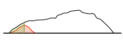
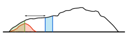
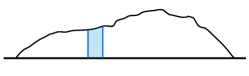
dist. $\varepsilon$
                                                            mass $\mathnormal{\Delta}$
 
(a)                                   (b)                                   (c)

Figure 1. (a) The solution is given by $v$ (black) minus $h$ (red); upper barrier is obtained by removing the leftmost mass of size $j_{0}=\|h\|_{1}$ from $v$ (green). (b) Removing mass of size $j_{0}$ (blue), located $\varepsilon$ away from the mass in green. (c) Removing instead mass of size $j_{0}$ (blue) after leaving mass of size $\mathnormal{\Delta}$ on the left, to obtain a lower barrier which can be iterated.

3.4. Upper barriers

These are defined using a removal mechanism that operates at discrete times $n\delta$, $n\in{\mathbb{N}}$. Given $\delta$, consider the time interval $[(n-1)\delta,n\delta]$. The mass injected during this interval adds the term $S*\alpha(\cdot,n\delta;(n-1)\delta)$ to the density at $n\delta$. Hence let the ‘paste’ operator be defined, for $u\in L_{1}({\mathbb{R}},{\mathbb{R}}_{+})$, by

$$P^{(\delta)}_{n}u=u+S*\alpha(\cdot,n\delta;(n-1)\delta).$$

The mass removed during the said interval is of size $J_{n\delta}-J_{(n-1)\delta}$. However, more relevant is the size this mass would grow to be had it not been removed, namely

$$j_{n}(\delta):=\int_{[(n-1)\delta,n\delta]}e^{\kappa(n\delta-s)}dJ_{s}.$$

Accordingly, let $C^{(\delta)}_{n}=C_{j_{n}(\delta)}$.

The upper barriers are defined for each $\delta>0$ and $n\in{\mathbb{N}}$ by setting $u^{(\delta,+)}_{0}=\xi_{0}$ and

$$u^{(\delta,+)}_{n\delta}=C^{(\delta)}_{n}P^{(\delta)}_{n}S_{\delta}u^{(\delta,+)}_{(n-1)\delta},\qquad n\in{\mathbb{N}}.$$

Note that for $n=1$ and $n\geq 2$, the function $S_{\delta}u^{(\delta,+)}_{(n-1)\delta}$ above is defined via (3.5) and, respectively, (3.4). For the barriers to be well defined one must have

(3.9) $$P^{(\delta)}_{n}S_{\delta}u^{(\delta,+)}_{(n-1)\delta}\in H_{j_{n}(\delta)}.$$

We sometimes use the notation $u_{t}$ for $u(\cdot,t)$ as we do in the following.

Proposition 3.6.

Fix $\delta>0$. Then (3.9) holds for all $n\in{\mathbb{N}}$, and consequently the upper barriers are well defined. Moreover, let $(u,\beta)$ be a solution to (2.10). Then for $n\in{\mathbb{N}}$,

$$u_{n\delta}\preccurlyeq u^{(\delta,+)}_{n\delta}.$$

Proof.

Recall that by Assumption 2.2, $m_{t}>0$ for all $t$, where $m_{t}$ is given by (2.6). The $L_{1}$ norm of $u^{(\delta,+)}$ satisfies

$$\|u^{(\delta,+)}_{n\delta}\|_{1}=\|u^{(\delta,+)}_{(n-1)\delta}\|_{1}e^{\kappa\delta}+\int_{[(n-1)\delta,n\delta]}e^{\kappa(n\delta-s)}dI_{s}-\int_{[(n-1)\delta,n\delta]}e^{\kappa(n\delta-s)}dJ_{s},$$

so long as the RHS above is positive. By induction on $n$, this expression gives $\|u^{(\delta,+)}_{n\delta}\|_{1}=m_{n\delta}>0$, completing the proof of the first assertion. Note by a simple induction argument, the definition of $j_{n}(\delta)$ and Lemma 3.3, that $\|u_{n\delta}\|_{1}=\|u_{n\delta}^{(\delta,+)}\|_{1}$.

The main claim is also proved by induction. For $n-1\geq 1$, assume $f\preccurlyeq g$ where $f=u_{(n-1)\delta}$ and $g=u^{(\delta,+)}_{(n-1)\delta}$; for $n-1=0$, $f=g=\xi_{0}$. Write $C$, $P$ and $S$ for $C^{(\delta)}_{n}$, $P^{(\delta)}_{n}$ and $S_{\delta}$, resp. We have $u^{(\delta,+)}_{n\delta}=CPSg$. Moreover, by Lemma 3.3, $u_{n\delta}=PSf-h$, where

$$h(y)=\int_{{\mathbb{R}}\times[(n-1)\delta,n\delta]}\mathfrak{s}_{n\delta-s}(x,y)\beta(dx,ds).$$

Hence the proof will be complete once $PSf-h\preccurlyeq CPSg$ is shown.

By Lemma 3.5(i,ii), $C$ preserves $\preccurlyeq$ and one has $S\tilde{u}\preccurlyeq S\tilde{v}$ whenever $\tilde{u}\preccurlyeq\tilde{v}$ and $\|\tilde{u}\|_{1}=\|\tilde{v}\|_{1}$. It is trivial that this is also true for $P$. Denote $w=PSf$. Suppose one shows $w-h\preccurlyeq Cw$. Then

$$w-h\preccurlyeq Cw=CPSf\preccurlyeq CPSg,$$

where in the last inequality one uses $Sf=Sg$ for $n-1=0$ and $\|f\|_{1}=\|g\|_{1}$ for $n-1\geq 1$. Thus the proof would be complete.

It thus suffices to show $w-h\preccurlyeq Cw$. The function $w-h$ is nonnegative (as required by the definition of a solution) and $\int h=j_{n}(\delta)$. Hence $w-h\preccurlyeq Cw$ by Lemma 3.5(iii), and the proof is complete. ∎

3.5. Lower barriers

The lower barriers are defined for ${\hat{\delta}}=(\mathnormal{\Delta},\delta)\in(0,\infty)^{2}$ and $n\in{\mathbb{N}}$ as follows. Let

$$C^{({\hat{\delta}})}_{n}=C_{\mathnormal{\Delta},j_{n}(\delta)}.$$

Set $u^{({\hat{\delta}},-)}_{0}=\xi_{0}$ and $\ell_{0,{\hat{\delta}}}=0$, and for $n\in{\mathbb{N}}$,

(3.10) $$u^{({\hat{\delta}},-)}_{n\delta}=C^{({\hat{\delta}})}_{n}P^{(\delta)}_{n}S_{\delta}u^{({\hat{\delta}},-)}_{(n-1)\delta},\qquad\ell_{n,{\hat{\delta}}}=e^{\kappa\delta}\ell_{n-1,{\hat{\delta}}}+\begin{cases}j_{n}(\delta)&\text{if }(n-1)\delta<t_{0},\\ e^{-\mathnormal{\Delta}^{5}/\delta}j_{n}(\delta)&\text{if }(n-1)\delta\geq t_{0},\end{cases}$$

where $t_{0}>0$ is fixed. Once again, for the definition to be valid, one must assure that for all $n\in{\mathbb{N}}$,

(3.11) $$P^{(\delta)}_{n}S_{\delta}u^{({\hat{\delta}},-)}_{(n-1)\delta}\in H_{\mathnormal{\Delta}+j_{n}(\delta)}.$$

Proposition 3.7.

For $\mathnormal{\Delta}\in(0,\varepsilon_{0})$ and $\delta>0$, (3.11) holds for all $n$ and consequently the lower barriers are well defined. Moreover, let $0<t_{0}<T$ be given. Then there exists $\mathnormal{\Delta}_{0}\in(0,\varepsilon_{0})$ such that for every $\mathnormal{\Delta}\in(0,\mathnormal{\Delta}_{0})$ there exists $\delta_{0}>0$ such that for $\delta\in(0,\delta_{0})$ and $n\in{\mathbb{N}}$ satisfying $n\delta\leq T$ one has

$$u^{({\hat{\delta}},-)}_{n\delta}\preccurlyeq u_{n\delta}{\rm\ mod\ }\ell_{n,{\hat{\delta}}}$$

whenever $(u,\beta)$ is a solution to (2.10). Furthermore, for $n\in{\mathbb{N}}$, $n\delta\leq T$ one has

(3.12) $$\ell_{n,{\hat{\delta}}}\leq e^{\kappa(T+\delta)}(J_{t_{0}+\delta}+e^{-\mathnormal{\Delta}^{5}/\delta}J_{T}).$$

Given $\gamma\in{\mathcal{M}}_{+,{\rm loc}}({\mathbb{R}}\times{\mathbb{R}}_{+})$ and $[t_{1},t_{2}]\subset{\mathbb{R}}_{+}$, the supremum of the support of the measure $\tilde{\gamma}(\cdot)=\gamma(\cdot\times[t_{1},t_{2}])$ is denoted by $\rho^{*}(\gamma;[t_{1},t_{2}])$. Recall $c_{*}$ from (3.2) and denote $c^{*}=2/c_{*}$.

Lemma 3.8.

Given a solution $(u,\beta)$, $\delta>0$ and $n\in{\mathbb{N}}$, denote $\rho_{n,\delta}=\rho^{*}(\beta;[(n-1)\delta,n\delta])$. Then for $n\geq 2$,

$$\rho_{n,\delta}\leq b(n,\delta,u_{(n-1)\delta}):=\mathnormal{\Lambda}_{c^{*}j_{n}(\delta)}(u_{(n-1)\delta}),\quad\text{provided\ \ $u_{(n-1)\delta}\in H_{c^{*}j_{n}(\delta)}$ and $j_{n}(\delta)>0$.}$$

Proof.

We consider only $n=2$; the proof for $n>2$ is similar. Fix $\delta$ and a solution $(u,\beta)$. Arguing by contradiction, assume $\rho_{2,\delta}>b=b(2,\delta,u_{\delta})=\mathnormal{\Lambda}_{c^{*}j_{2}(\delta)}(u_{\delta})$ (the latter is well defined and finite by the assumption $u_{\delta}\in H_{c^{*}j_{2}(\delta)}$). It follows that $\beta((b,\infty)\times[\delta,2\delta])>0$. Because $\beta$ does not charge ${\mathbb{R}}\times\{\delta\}$, it follows that $\theta:=\beta((b,\infty)\times(\delta,2\delta])>0$.

Let us show using (2.10)(ii) that there exists $t\in(\delta,2\delta]$ such that $U(b,t)=0$. If this statement is false, namely $U(b,t)>0$ for all $t\in(\delta,2\delta]$, then

$$\beta(U>0)\geq\int_{(b,\infty)\times(\delta,2\delta]}1_{\{U(x,t)>0\}}\beta(dx,dt)\geq\int_{(b,\infty)\times(\delta,2\delta]}1_{\{U(b,t)>0\}}\beta(dx,dt)=\theta>0,$$

contradicting (2.10)(ii).

Fix such $t\in(\delta,2\delta]$. We now appeal to identity (3.7) with $\tau=\delta$. Denoting the last term there by $h(y)=\int_{{\mathbb{R}}\times[\delta,t]}\mathfrak{s}_{t-s}(x,y)\beta(dx,ds)$,

$$\int_{-\infty}^{b}h(y)dy\leq\int_{-\infty}^{\infty}h(y)dy=\int_{[\delta,t]}e^{\kappa(t-s)}dJ_{s}\leq\int_{[\delta,2\delta]}e^{\kappa(2\delta-s)}dJ_{s}=j_{2}(\delta).$$

Since $U(b,t)=0$, we have for the first term in (3.7),

$$\int_{-\infty}^{b}\int_{\mathbb{R}}\mathfrak{s}_{t-\delta}(x,y)u(x,\delta)dx\,dy\leq\int_{-\infty}^{b}h(y)dy\leq j_{2}(\delta).$$

Using (3.2), $\int_{-\infty}^{x}\mathfrak{s}_{t-\delta}(x,y)dy\geq\int_{-\infty}^{x}\mathfrak{p}_{t-\delta}(x,y)dy\geq c_{*}$ for all $x$, hence

$$j_{2}(\delta) \geq\int_{x\in(-\infty,b]}\int_{y\in(-\infty,b]}\mathfrak{s}_{t-\delta}(x,y)u(x,\delta)dy\,dx$$

$$\geq c_{*}\int_{-\infty}^{b}u(x,\delta)dx=c_{*}c^{*}j_{2}(\delta)=2j_{2}(\delta),$$

a contradiction due to the assumption $j_{2}(\delta)>0$. This proves the claim. ∎

Proof of Proposition 3.7.

The proof of (3.11) is similar to the proof of the analogous statement from Proposition 3.6. Also as in that proof, the $L_{1}$ norm of the solution and the barrier at $n\delta$ are equal. As for (3.12), fix $0<t_{0}<T$. Denoting $\chi_{n}=1_{(n-1)\delta<t_{0}}+e^{-\mathnormal{\Delta}^{5}/\delta}$, it follows from (3.10) that

$$\ell_{n,{\hat{\delta}}}\leq e^{\kappa\delta}\ell_{n-1,{\hat{\delta}}}+j_{n}(\delta)\chi_{n}.$$

By induction, $\ell_{n,{\hat{\delta}}}\leq e^{n\kappa\delta}\sum_{i=1}^{n}j_{i}(\delta)\chi_{i}$. Using $j_{n}(\delta)\leq e^{\kappa\delta}(J_{n\delta}-J_{(n-1)\delta})$ and $n\delta\leq T$,

$$\ell_{n,{\hat{\delta}}}\leq e^{\kappa(T+\delta)}(J_{t_{0}+\delta}+e^{-\mathnormal{\Delta}^{5}/\delta}J_{T}),$$

as claimed.

We turn to the main assertion. Assume that $\mathnormal{\Delta}<\varepsilon_{0}/2$. Arguing by induction, assume that $f\preccurlyeq g{\rm\ mod\ }\ell_{n-1,{\hat{\delta}}}$, where

$$f=u^{({\hat{\delta}},-)}_{(n-1)\delta},\qquad g=u_{(n-1)\delta},$$

when $n-1\geq 1$ and $f=g=\xi_{0}$ when $n-1=0$. Write $C$, $P$ and $S$ for $C^{({\hat{\delta}})}_{n}$, $P^{(\delta)}_{n}$ and $S_{\delta}$, respectively. Then $u^{({\hat{\delta}},-)}_{n\delta}=CPSf$, and by Lemma 3.3, $u_{n\delta}=PSg-h$, where

$$h(y)=\int_{{\mathbb{R}}\times[(n-1)\delta,n\delta]}\mathfrak{s}_{n\delta-s}(x,y)\beta(dx,ds).$$

By Lemma 3.5(i), $PSf\preccurlyeq PSg$ mod $e^{\kappa\delta}\ell_{n-1,{\hat{\delta}}}$. If $(n-1)\delta<t_{0}$ we therefore have, for any $r$,

$$u^{({\hat{\delta}},-)}_{n\delta}[r,\infty)=CPSf[r,\infty) \leq PSf[r,\infty)$$

$$\leq PSg[r,\infty)+e^{\kappa\delta}\ell_{n-1,{\hat{\delta}}}$$

$$\leq PSg[r,\infty)-h[r,\infty)+\|h\|_{1}+e^{\kappa\delta}\ell_{n-1,{\hat{\delta}}}$$

$$=u_{n\delta}[r,\infty)+j_{n}(\delta)+e^{\kappa\delta}\ell_{n-1,{\hat{\delta}}}$$

$$=u_{n\delta}[r,\infty)+\ell_{n,{\hat{\delta}}},$$

which gives the claimed estimate.

In what follows, $(n-1)\delta\geq t_{0}$. In particular, $n\geq 2$. In view of the lower bound on $m_{t}=\|u(\cdot,t)\|_{1}$, $t\in[0,T]$ and the continuity of $J$, we may assume that $\delta$ is so small that the condition $u_{(n-1)\delta}\in H_{c^{*}j_{n}(\delta)}$ holds for all $n\geq 2$, $n\delta\leq T$. As a result, the bound asserted in Lemma 3.8 is valid provided merely that $j_{n}(\delta)>0$. Moreover, by Lemma 3.3 there exists a constant $c_{\infty}$ such that for any solution $(u,\beta)$, $\|u(\cdot,t)\|_{\infty}<c_{\infty}$, $t\in[t_{0},T]$. Using the induction assumption and Lemma 3.5(iv),

$$u^{({\hat{\delta}},-)}_{n\delta}=CPSf\preccurlyeq CPSg{\rm\ mod\ }e^{\kappa\delta}\ell_{n-1,{\hat{\delta}}}.$$

Denote $w=PSg$. Suppose

(3.13) $$Cw\preccurlyeq w-h{\rm\ mod\ }\varepsilon,\text{ where $\varepsilon=\ell_{n,{\hat{\delta}}}-e^{\kappa\delta}\ell_{n-1,{\hat{\delta}}}=e^{-\mathnormal{\Delta}^{5}/\delta}j_{n}(\delta)$}.$$

Then $u^{({\hat{\delta}},-)}_{n\delta}\preccurlyeq w-h=u_{n\delta}{\rm\ mod\ }\ell_{n,{\hat{\delta}}}$, which completes the proof. It remains to show (3.13).

First, if $j_{n}(\delta)=0$ then $\varepsilon=0$ and (3.13) holds because $C={\tt id}$, $h=0$, and so $Cw=w=w-h$. Next assume $j_{n}(\delta)>0$. Denote $j=j_{n}(\delta)$ and $b=\mathnormal{\Lambda}_{c^{*}j_{n}(\delta)}(g)=\mathnormal{\Lambda}_{c^{*}j}(g)$. By Lemma 3.8, $\rho_{n,\delta}\leq b$. Write $h=h_{1}+h_{2}$, where

$$h_{1}(y)=h(y)1_{\{y>b+\mathnormal{\Delta}^{2}\}},\qquad h_{2}(y)=h(y)1_{\{y\leq b+\mathnormal{\Delta}^{2}\}}.$$

Because $\rho_{n,\delta}\leq b$, we have

$$h(y)=\int_{(-\infty,b]\times[(n-1)\delta,n\delta]}\mathfrak{s}_{n\delta-s}(x,y)\beta(dx,ds).$$

Without loss of generality, $e^{\kappa\delta}<2$, thus $\mathfrak{s}_{t}\leq 2\mathfrak{p}_{t}$ for $t\leq\delta$. Hence in view of Lemma 3.2, $\mathfrak{s}_{t}(0,[a,\infty))\leq c_{3}e^{-c_{4}a^{2}/t}$ for $a>t^{1/2}>0$, where $c_{3},c_{4}>0$ depend only on $\hat{c}_{1},\hat{c}_{2}$ of the lemma. This gives

$$\|h_{1}\|_{1}\leq c_{3}\int_{(-\infty,b]\times[(n-1)\delta,n\delta]}e^{-c_{4}\mathnormal{\Delta}^{4}/(n\delta-s)}\beta(dx,ds)\leq c_{3}e^{-c_{4}\mathnormal{\Delta}^{4}/\delta}j,$$

provided $\delta<\mathnormal{\Delta}^{4}$. If we further require $\mathnormal{\Delta}<c_{4}$ then for all sufficiently small $\delta$,

(3.14) $$\|h_{1}\|_{1}\leq e^{-\mathnormal{\Delta}^{5}/\delta}j=\varepsilon.$$

Recall that $\|h\|_{1}=j$ and let $q\in(0,1]$ be defined by $\|h_{2}\|_{1}=qj$. Then $q\geq 1-e^{-\mathnormal{\Delta}^{5}\delta}$. Let us argue that it suffices to show

(3.15) $$b+\mathnormal{\Delta}^{2}=\mathnormal{\Lambda}_{c^{*}j}(g)+\mathnormal{\Delta}^{2}\leq\mathnormal{\Lambda}_{\mathnormal{\Delta}}(w)$$

in order to prove (3.13). By definition, $h_{2}$ is supported to the left of $b+\mathnormal{\Delta}^{2}$. On the other hand, $C_{\mathnormal{\Delta},qj}w=w-\tilde{h}$, where $\|\tilde{h}\|_{1}=qj$ and $\tilde{h}$ is supported to the right of $\mathnormal{\Lambda}_{\mathnormal{\Delta}}(w)$. Thus using $\|\tilde{h}\|_{1}=\|h_{2}\|_{1}$, it follows from (3.15) that $C_{\mathnormal{\Delta},qj}w\preccurlyeq w-h_{2}=w-h+h_{1}$. In view of (3.14) this gives

$$C_{\mathnormal{\Delta},qj}w\preccurlyeq w-h{\rm\ mod\ }\varepsilon.$$

Because $Cw=C_{\mathnormal{\Delta},j}w\leq C_{\mathnormal{\Delta},qj}w$ pointwise, one has $Cw\preccurlyeq C_{\mathnormal{\Delta},qj}w$. Hence (3.13) follows.

It remains to show (3.15). Because $t_{0}\leq(n-1)\delta\leq T$, the bound $\|g\|_{\infty}\leq c_{\infty}$ is valid. By making $\mathnormal{\Delta}$ smaller if needed, assume $2c_{\infty}\mathnormal{\Delta}^{2}<\mathnormal{\Delta}/6$. Then for all $\delta$ so small that $c^{*}j<\mathnormal{\Delta}/6$ (simultaneously over $n$),

(3.16) $$\mathnormal{\Lambda}_{\mathnormal{\Delta}/3}(g)\geq\mathnormal{\Lambda}_{c^{*}j}(g)+2\mathnormal{\Delta}^{2}.$$

Next we argue that for all small $\delta$,

(3.17) $$\mathnormal{\Lambda}_{2\mathnormal{\Delta}/3}(Sg)\geq\theta:=\mathnormal{\Lambda}_{\mathnormal{\Delta}/3}(g)-\mathnormal{\Delta}^{2}.$$

To show this we must to show $(Sg)(-\infty,\theta]\leq 2\mathnormal{\Delta}/3$. Let $g=g_{1}+g_{2}=\widehat{C}_{\mathnormal{\Delta}/3}g+C_{\mathnormal{\Delta}/3}g$. Because $\|g_{1}\|_{1}=\mathnormal{\Delta}/3$, we have $\|Sg_{1}\|_{1}\leq e^{\kappa\delta}\mathnormal{\Delta}/3\leq\mathnormal{\Delta}/2$, and

$$(Sg)(-\infty,\theta]=(Sg_{1})(-\infty,\theta]+(Sg_{2})(-\infty,\theta]\leq\mathnormal{\Delta}/2+\|g_{2}\|_{1}e^{\kappa\delta}\mathfrak{p}_{\delta}(x_{0},(-\infty,\theta]),$$

where $x_{0}=\mathnormal{\Lambda}_{\mathnormal{\Delta}/3}(g)$, owing to the fact that $\mathfrak{p}_{\delta}(y,(-\infty,\theta])$ is monotone decreasing in $y$ for $y>\theta$. Recalling that $\|g\|_{1}=\|u_{(n-1)\delta}\|_{1}=m_{(n-1)\delta}\leq\|m\|^{*}_{T}$ and using again Lemma 3.2, the last term in the above display is bounded by

$$2\hat{c}_{1}\|m\|^{*}_{T}\int_{-\infty}^{x_{0}-\mathnormal{\Delta}^{2}}\delta^{-1/2}e^{-\hat{c}_{2}(x_{0}-y)^{2}\delta^{-1}}dy,$$

which is smaller than $\mathnormal{\Delta}/6$ for all sufficiently small $\delta$. This shows $(Sg)(-\infty,\theta]\leq 2\mathnormal{\Delta}/3$ hence (3.17).

For $\pi:=S*\alpha(\cdot,n\delta;(n-1)\delta)$ we have $\|\pi\|_{1}\leq e^{\kappa\delta}(I_{n\delta}-I_{(n-1)\delta})$. Hence for all small $\delta$, $\|\pi\|_{1}<\mathnormal{\Delta}/3$. As a result,

$$\mathnormal{\Lambda}_{\mathnormal{\Delta}}(w)=\mathnormal{\Lambda}_{\mathnormal{\Delta}}(PSg)=\mathnormal{\Lambda}_{\mathnormal{\Delta}}(Sg+\pi)\geq\mathnormal{\Lambda}_{2\mathnormal{\Delta}/3}(Sg).$$

Combining this with (3.16) and (3.17) gives (3.15), and the proof is complete. ∎

3.6. Proof of uniqueness

The last step is showing that the lower and upper barriers become close upon taking $\delta\to 0$ then $\mathnormal{\Delta}\to 0$ and finally $t_{0}\to 0$.

Proposition 3.9.

Fix $0<t_{0}<T$. Let $\mathnormal{\Delta}_{0}$ and $\delta_{0}=\delta_{0}(\mathnormal{\Delta}_{0})$ be as in Proposition 3.7. Then for $\mathnormal{\Delta}\in(0,\mathnormal{\Delta}_{0})$, $\delta\in(0,\delta_{0})$ and $n\in{\mathbb{N}}$, $n\delta\leq T$, one has

$$u^{(\delta,+)}_{n\delta}\preccurlyeq u^{({\hat{\delta}},-)}_{n\delta}{\rm\ mod\ }e^{n\kappa\delta}\mathnormal{\Delta}.$$

Proof.

By induction. Recall $u^{(\pm)}_{0}=\xi_{0}$. Assume $u^{(\delta,+)}_{(n-1)\delta}\preccurlyeq u^{({\hat{\delta}},-)}_{(n-1)\delta}{\rm\ mod\ }e^{(n-1)\kappa\delta}\mathnormal{\Delta}$. Then

$$P^{(\delta)}_{n}S_{\delta}u^{(\delta,+)}_{(n-1)\delta}\preccurlyeq P^{(\delta)}_{n}S_{\delta}u^{({\hat{\delta}},-)}_{(n-1)\delta}{\rm\ mod\ }e^{n\kappa\delta}\mathnormal{\Delta},$$

where, for $n-1=0$, this is true because both sides of the inequality are equal, and otherwise this is a consequence of the induction assumption and Lemma 3.5(i), recalling that the $L_{1}$ norm of the upper and lower barriers are equal for each $n$. For the same reason, Lemma 3.5(vi) also applies, and gives

$$C^{(\delta)}_{n}P^{(\delta)}_{n}S_{\delta}u^{(\delta,+)}_{(n-1)\delta}\preccurlyeq C^{({\hat{\delta}})}_{n}P^{(\delta)}_{n}S_{\delta}u^{({\hat{\delta}},-)}_{(n-1)\delta}{\rm\ mod\ }e^{n\kappa\delta}\mathnormal{\Delta},$$

that is, $u^{(\delta,+)}_{n\delta}\preccurlyeq u^{({\hat{\delta}},-)}_{n\delta}{\rm\ mod\ }e^{n\kappa\delta}\mathnormal{\Delta}$. This completes the proof. ∎

Proof of Theorem 3.1.

Once uniqueness is established for the $u$ component of the solution $(u,\beta)$, uniqueness of the $\beta$ component follows from (4.1). By Remark 3.4 it suffices to prove uniqueness of solutions $(u,\beta)$ in which $u$ is the version given by Lemma 3.3. To show uniqueness of the $u$ component, argue by contradiction and assume that $(u^{i},\beta^{i})$, $i=1,2$ are two solutions where $u^{1}$ and $u^{2}$ are distinct. Then there exist $t>0$ and $r\in{\mathbb{R}}$ such that, say, $u^{1}_{t}[r,\infty)<u^{2}_{t}[r,\infty)$. Fix such $t$ and $r$. Denote $\delta_{n}=tn^{-1}$ for $n\in{\mathbb{N}}$. Let $0<t_{0}<t$. Then by Propositions 3.6 and 3.7, for every small $\mathnormal{\Delta}>0$ there exists $n_{0}$ such that for $n>n_{0}$,

$$u^{(\mathnormal{\Delta},\delta_{n},-)}_{t}[r,\infty)-\ell_{n,\mathnormal{\Delta},\delta_{n}}\leq u^{1}_{t}[r,\infty)<u^{2}_{t}[r,\infty)\leq u^{(\mathnormal{\Delta},+)}_{t}[r,\infty).$$

By Proposition 3.9,

$$u^{(\mathnormal{\Delta},+)}_{t}[r,\infty)\leq u^{(\mathnormal{\Delta},\delta_{n},-)}_{t}[r,\infty)+e^{\kappa t}\mathnormal{\Delta}.$$

Using these two inequalities and then the bound from (3.12),

$$0<u^{2}_{t}[r,\infty)-u^{1}_{t}[r,\infty)\leq e^{\kappa t}\mathnormal{\Delta}+\ell_{n,\mathnormal{\Delta},\delta_{n}}\leq e^{\kappa t}\mathnormal{\Delta}+e^{\kappa(t+\delta_{n})}(J_{t_{0}+\delta_{n}}+e^{-\mathnormal{\Delta}^{5}/\delta_{n}}J_{t}).$$

On taking $n\to\infty$, then $\mathnormal{\Delta}\downarrow 0$ and finally $t_{0}\downarrow 0$, the expression on the right converges to zero, a contradiction. ∎

4. Injection-branching-selection: Convergence

In this section the convergence result is proved based on the uniqueness result, yielding the proof of Theorem 2.4. Throughout, the assumptions of Theorem 2.4 hold. The main steps are as follows. In Lemma 4.1, the normalized processes are shown to satisfy a version of equation (2.9) with an error term. Lemma 4.2 establishes tightness of these processes. Existence of a measurable density for any limit point of the sequence $\bar{\xi}^{N}$ is shown in Lemma 4.3 based on a result from [17]. In Lemma 4.4, the final, crucial step shows that the complementarity condition is preserved under the limit.

4.1. Limit laws and the parabolic equation

This subsection contains the first three of the aforementioned steps toward convergence. Some notation used here is as follows. Let $J^{\#,N}_{t}=\beta^{N}({\mathbb{R}}\times[0,t])$ denote the counting process for removals, and note that, by construction, $J^{\#,N}_{t}=J^{N}_{t}$ holds on the event $\{\inf_{s\leq t}m^{N}_{s}\geq 1\}$. Let

$$Y^{N}_{t}=\sum_{i\in{\mathcal{S}}}1_{\{\sigma^{i}\leq t\}}(\pi^{i}_{t\wedge\tau^{i}}-\pi^{i}_{\sigma^{i}})$$

be the number of births during $[0,t]$, and let its macroscopic counterpart be given by $Y_{t}=\kappa\int_{0}^{t}m_{s}ds$. Denote $R^{N}_{T}=N+I^{N}_{T}$ and note that the set ${\mathcal{R}}^{N}_{T}=\{(j,0):j\leq R^{N}_{T}\}$ consists of all root particles appearing by time $T$.

Recall that a solution to (2.8) is defined via (2.9), which in the case of (2.10)(i) takes the form

(4.1) $$-\int_{0}^{\infty}(\partial_{t}\varphi+{\mathcal{L}}\varphi,u)dt=\int_{{\mathbb{R}}}\varphi(\cdot,0)d\xi_{0}+\int_{{\mathbb{R}}\times{\mathbb{R}}_{+}}\varphi d\alpha-\int_{{\mathbb{R}}\times{\mathbb{R}}_{+}}\varphi d\beta,$$

for $\varphi\in C_{c}^{\infty}({\mathbb{R}}\times{\mathbb{R}}_{+})$. The relation of the particle system to this equation is established by showing that if $(\xi,\beta)$ is a limit point of $(\bar{\xi}^{N},\bar{\beta}^{N})$ then

(4.2) $$-\int_{0}^{\infty}\langle\partial_{t}\varphi+{\mathcal{L}}\varphi,\xi_{t}\rangle dt=\int_{{\mathbb{R}}}\varphi(\cdot,0)d\xi_{0}+\int_{{\mathbb{R}}\times{\mathbb{R}}_{+}}\varphi d\alpha-\int_{{\mathbb{R}}\times{\mathbb{R}}_{+}}\varphi d\beta.$$

Lemma 4.1.

i. Let $\varphi\in C_{c}^{\infty}({\mathbb{R}}\times{\mathbb{R}}_{+})$ and let $T$ be such that $\varphi(\cdot,t)=0$ for all $t\geq T$. Then

$$-\int_{0}^{\infty}\langle(\partial_{t}\varphi+{\mathcal{L}}\varphi)(\cdot,t),\bar{\xi}^{N}_{t}\rangle dt=\langle\varphi(\cdot,0),\bar{\xi}^{N}_{0}\rangle+\int_{{\mathbb{R}}\times{\mathbb{R}}_{+}}\varphi d\bar{\alpha}^{N}-\int_{{\mathbb{R}}\times{\mathbb{R}}_{+}}\varphi d\bar{\beta}^{N}+\bar{M}^{N}_{T},$$

where $\bar{M}^{N}_{t}$ is an $\{{\mathcal{F}}^{N}_{t}\}$-martingale starting at zero, with quadratic variation

(4.3) $$[\bar{M}^{N}]_{t}\leq cN^{-1}\Big{(}\int_{0}^{t}\bar{m}^{N}_{s}ds+\bar{Y}^{N}_{t}\Big{)},$$

where $c$ depends only on $\varphi$ and $\mathfrak{c}$.

ii. One has

$$\bar{m}^{N}_{t}=1+\kappa\int_{0}^{t}\bar{m}^{N}_{s}ds+\bar{I}^{N}_{s}-\bar{J}^{\#,N}_{t}+\bar{M}^{\#,N}_{t},$$

where, with $c$ as above, $\bar{M}^{\#,N}_{t}$ is an $\{{\mathcal{F}}^{N}_{t}\}$-martingale starting at zero, and

$$[\bar{M}^{\#,N}]_{t}\leq cN^{-1}\bar{Y}^{N}_{t}.$$

iii. As $N\to\infty$, $(\bar{m}^{N},\bar{Y}^{N},\bar{I}^{N},\bar{J}^{N},\bar{J}^{\#,N})\to(m,Y,I,J,J)$ in probability.

iv. Suppose that $(\xi_{0},\xi,\alpha,\beta)$ is a subsequential limit of $(\bar{\xi}^{N}_{0},\bar{\xi}^{N},\bar{\alpha}^{N},\bar{\beta}^{N})$. Then the former tuple satisfies (4.2) a.s.

Proof.

i. Note that $\sigma^{i}$ and $\tau^{i}$ are $\{{\mathcal{F}}^{N}_{t}\}$-stopping times and recall that $B^{i}$ and $\hat{\pi}^{i}$ are martingales on this filtration. By Itô’s formula, for each $i\in{\mathcal{S}}$, on the event $\{t\geq\sigma^{i}\}$,

$$\varphi(X^{i}_{t\wedge\tau^{i}},t\wedge\tau^{i}) =\varphi(x^{i},\sigma^{i})+\int_{\sigma^{i}}^{t\wedge\tau^{i}}(\partial_{t}\varphi+\mathfrak{b}\partial_{x}\varphi+\mathfrak{a}\partial_{x}^{2}\varphi)(X^{i}_{s},s)ds+\int_{\sigma^{i}}^{t\wedge\tau^{i}}(\mathfrak{c}\partial_{x}\varphi)(X^{i}_{s},s)dB^{i}_{s}$$

(4.4) $$=\varphi(x^{i},\sigma^{i})+\int_{\sigma^{i}}^{t\wedge\tau^{i}}(\partial_{t}\varphi+\mathfrak{b}\partial_{x}\varphi+\mathfrak{a}\partial_{x}^{2}\varphi)(X^{i}_{s},s)ds+M^{N,i,1}_{t},$$

where

$$M^{N,i,1}_{t}=1_{\{\sigma^{i}\geq t\}}\int_{\sigma^{i}}^{t\wedge\tau^{i}}(\mathfrak{c}\partial_{x}\varphi)(X^{i}_{s},s)dB^{i}_{s}.$$

Given $i$, the sum of evaluations of $\varphi$ over birth location-epochs of particles born directly from particle $i$ between time $0$ and $t$ is given by

$$1_{\{t\geq\sigma^{i}\}}\int_{\sigma^{i}}^{t\wedge\tau^{i}}\varphi(X^{i}_{s},s)d\pi^{i}_{s}.$$

Summing this expression over $i\in{\mathcal{S}}$ gives the sum of evaluations of $\varphi$ over all birth location-epochs during that time interval, i.e.,

$$\sum\varphi(x^{i},\sigma^{i}) =\sum_{i\in{\mathcal{S}}}1_{\{t\geq\sigma^{i}\}}\int_{\sigma^{i}}^{t\wedge\tau^{i}}\varphi(X^{i}_{s},s)d\pi^{i}_{s}$$

$$=\sum_{i\in{\mathcal{S}}}1_{\{t\geq\sigma_{i}\}}\Big{[}\int_{\sigma^{i}}^{t\wedge\tau^{i}}\varphi(X^{i}_{s},s)\kappa ds+M^{N,i,2}_{t}\Big{]},$$

where the sum on the left extends over $i=(j,k)\in{\mathcal{S}}^{N}_{t}$ such that $j\geq 1$ (corresponding to births), and

$$M^{N,i,2}_{t}=1_{\{t\geq\sigma^{i}\}}\int_{\sigma^{i}}^{t\wedge\tau^{i}}\varphi(X^{i}_{s},s)d\hat{\pi}^{i}_{s}.$$

Therefore, summing (4.1) over all $i$ such that $\sigma^{i}\leq t$ and normalizing gives

$$\int_{{\mathbb{R}}\times[0,t]}\varphi d\bar{\beta}^{N} =\int_{\mathbb{R}}\varphi(\cdot,0)d\bar{\xi}^{N}_{0}+\int_{{\mathbb{R}}\times[0,t]}\varphi d\bar{\alpha}^{N}+\int_{0}^{t}\int_{\mathbb{R}}(\partial_{t}\varphi+{\mathcal{L}}\varphi)(x,t)\bar{\xi}^{N}_{t}(dx)dt+\bar{M}^{N}_{t},$$

where

$$\bar{M}^{N}_{t}=N^{-1}M^{N}_{t},\qquad M^{N}_{t}=\sum_{i\in{\mathcal{S}}}(M^{N,i,1}_{t}+M^{N,i,2}_{t}).$$

Take $t=T$ and replace the integration range ${\mathbb{R}}\times[0,T]$ to ${\mathbb{R}}\times{\mathbb{R}}_{+}$ recalling that $\varphi(x,t)=0$ for $t>T$. The bound (4.3) follows from $[M^{N,i,1}]_{t}\leq 1_{\{t\geq\sigma_{i}\}}\|\mathfrak{c}\|^{2}_{\infty}\|\partial_{x}\varphi\|^{2}_{\infty}(t\wedge\tau^{i}-\sigma^{i})$ and $[M^{N,i,2}]_{t}\leq 1_{\{t\geq\sigma_{i}\}}\|\varphi\|^{2}_{\infty}(\pi^{i}_{t\wedge\tau^{i}}-\pi^{i}_{\sigma^{i}})$ and the identities

$$\sum_{i\in{\mathcal{S}}}1_{\{t\geq\sigma^{i}\}}(t\wedge\tau^{i}-\sigma^{i})=\int_{0}^{t}\xi^{N}_{s}({\mathbb{R}})ds=\int_{0}^{t}m^{N}_{s}ds$$

and

(4.5) $$\sum_{i\in{\mathcal{S}}}1_{\{t\geq\sigma^{i}\}}(\pi^{i}_{t\wedge\tau^{i}}-\pi^{i}_{\sigma^{i}})=Y^{N}_{t}.$$

ii. We have $m^{N}_{t}=N+I^{N}_{t}+Y^{N}_{t}-J^{\#,N}_{t}$ by the definition of these processes. By (4.5),

(4.6) $$Y^{N}_{t}=\kappa\int_{0}^{t}m^{N}_{s}ds+\kappa M^{\#,N}_{t},\qquad\text{where}\qquad M^{\#,N}_{t}=\sum_{i\in{\mathcal{S}}}1_{\{t\geq\sigma^{i}\}}\int_{\sigma^{i}}^{t\wedge\tau^{i}}d\hat{\pi}^{i}_{s}.$$

The quadratic variation bound follows as in (i).

iii. Fix $T$. Recall $\varepsilon_{0}$ from Assumption 2.2. Consider the $\{{\mathcal{F}}^{N}_{t}\}$-stopping time $\theta^{N}=\inf\{t:\bar{I}^{N}_{t}\geq I_{T}+1\text{ or }\bar{m}^{N}_{t}\leq\varepsilon_{0}/2\}$. By (ii), using Gronwall’s lemma, ${\mathbb{E}}[\bar{m}^{N}_{t\wedge\theta^{N}}]\leq c$, where $c=c(T)$. Hence by (4.6), ${\mathbb{E}}[\bar{Y}^{N}_{t\wedge\theta^{N}}]\leq c$. Going back to (ii) gives that ${\mathbb{E}}[[\bar{M}^{\#,N}]_{T\wedge\theta^{N}}]\to 0$, hence $\|\bar{M}^{\#,N}\|^{*}_{T\wedge\theta^{N}}\to 0$ in probability. For $t\leq\theta^{N}$, one has $J^{\#,N}_{t}=J^{N}_{t}$. Thus using (2.6) and again Gronwall’s lemma, $\|\bar{m}^{N}-m\|^{*}_{T\wedge\theta^{N}}\to 0$ in probability. By the definition of $\varepsilon_{0}$, this shows that ${\mathbb{P}}(\theta^{N}<T)\to 0$. Because $T$ is arbitrary, this proves that $\bar{m}^{N}\to m$ and $\bar{J}^{\#,N}\to J$ in probability. As a result, by (4.6), $\bar{Y}^{N}\to Y$ in probability.

iv. In view of (i), it suffices to show that $\|\bar{M}^{N}\|^{*}_{T}\to 0$ in probability. However, this is an immediate consequence of (4.3) and (iii). ∎

The following point is used in the proof of the next two lemmas. One can construct an additional particle system in which there are no removals, based on the same stochastic primitives as in the original system, except $\tilde{\eta}^{l}=\infty$ for all $l$ in place of the original removal times $\eta^{l}$. In this particle system we use tilde notation for all the model ingredients, as in $\tilde{x}^{i}$, $\tilde{X}^{i}$, $\tilde{\sigma}^{i}$, with one exception: instead of $\tilde{\xi}^{N}$ we write $\zeta^{N}$ (and $\bar{\zeta}^{N}$ for its normalized version). Thus $\tilde{J}^{N}=0$, $\tilde{\beta}^{N}=0$ and $\tilde{\tau}^{i}=\infty$ for all $i$. The tilde system dominates the original system in several ways. For example, it is easy to see by a simple coupling that for every $A\in{\mathcal{B}}({\mathbb{R}})$ and $t\geq 0$, the random variable $\xi^{N}_{t}(A)$ is stochastically dominated by $\zeta^{N}_{t}(A)$.

Lemma 4.2.

The sequence of laws of $(\bar{\xi}^{N},\bar{\beta}^{N})$, $N\in{\mathbb{N}}$, is tight. For every subsequential limit $(\xi,\beta)$, one has ${\mathbb{P}}(\xi\in C({\mathbb{R}}_{+},{\mathcal{M}}_{+}({\mathbb{R}})))=1$.

Proof.

Both the $J_{1}$ topology over $D({\mathbb{R}}_{+},{\mathbb{R}})$ and the topology of local weak convergence we gave the space ${\mathcal{M}}_{+,\rm loc}({\mathbb{R}}\times{\mathbb{R}}_{+})$ are defined by convergence over finite time intervals. Hence in this proof we fix $T$ and consider all processes (respectively, measures) defined on ${\mathbb{R}}_{+}$ (on subsets of ${\mathbb{R}}\times{\mathbb{R}}_{+}$) as if they are defined on $[0,T]$ (on subsets of ${\mathbb{R}}\times[0,T]$), and with a slight abuse of notation still use the same notation. For example, $\beta^{N}$ will denote the restriction of the original random measure $\beta^{N}$ to subsets of ${\mathbb{R}}\times[0,T]$.

Moreover, recalling that $\bar{\alpha}^{N}({\mathbb{R}}\times[0,T])=\bar{I}^{N}_{T}\to I_{T}$ in probability, we may and will assume without loss of generality that the injections are truncated when their number reaches $c_{I}N$, where $c_{I}=I_{T}+1$. Hence, for all $N$ and $t\in[0,T]$, $I^{N}_{t}\leq c_{I}N$ a.s. Similarly, the removal measure is assumed without loss to be truncated when $J^{N}$ reaches $c_{J}N$, $c_{J}=J_{T}+1$.

Tightness may be argued separately for each component. Starting with $\bar{\beta}^{N}$, for $r>0$, denote $\mathbb{B}_{r,T}=[-r,r]\times[0,T]$, and for $n\in{\mathbb{N}}$, set

$$K_{n}(r)=\{\gamma\in{\mathcal{M}}_{+}({\mathbb{R}}\times[0,T]):|\gamma|\leq c_{J},\,\gamma(\mathbb{B}_{r,T}^{c})<n^{-1}\}.$$

Then by Prohorov’s theorem (see [12, Theorem A2.4.I] for a version for finite measures), for any $n_{0}$ and sequence $\{r_{n}\}$, the closure of $K_{\geq n_{0}}(\{r_{n}\}):=\cap_{n\geq n_{0}}K_{n}(r_{n})$ as a subset of ${\mathcal{M}}({\mathbb{R}}\times[0,T])$ endowed with the topology of weak convergence, is compact. Suppose we show that for every $n$ there exists $r_{n}$ such that

(4.7) $$\liminf_{N}{\mathbb{P}}(\bar{\beta}^{N}\in K_{n}(r_{n}))\geq 1-2^{-n}.$$

Given $\varepsilon>0$ let $n_{0}$ be such that $\sum_{n\geq n_{0}}2^{-n}<\varepsilon$. Then

$$\liminf_{N}{\mathbb{P}}(\bar{\beta}^{N}\in\overline{K_{\geq n_{0}}(\{r_{n}\})})>1-\varepsilon.$$

This would show that $\bar{\beta}^{N}$ are tight.

Toward showing (4.7), note that the removal space-time location of a particle is a point on the graph of the potential trajectory of that particle, hence

(4.8) $$\beta^{N}(\mathbb{B}_{r,T}^{c})\leq U^{N}_{r}:=\sum_{i\in{\mathcal{S}}^{N}_{T}}1_{\{\|X^{i}\|^{*}_{[\sigma^{i},T]}>r\}}.$$

If we let

$$\tilde{U}^{N}_{r}=\sum_{i\leq\tilde{\mathcal{S}}^{N}_{T}}1_{\{\|\tilde{X}\|^{*}_{[\tilde{\sigma}^{i},T]}>r\}},$$

then for each $N$ and $r$, the random variable $U^{N}_{r}$ is stochastically dominated by $\tilde{U}^{N}_{r}$, as follows by a simple coupling between the two particle systems. Recalling that $|\bar{\beta}^{N}|\leq c_{J}$, this shows

(4.9) $${\mathbb{P}}(\bar{\beta}^{N}\in K_{n}(r)^{c})={\mathbb{P}}(\bar{\beta}^{N}(\mathbb{B}_{r,T}^{c})\geq n^{-1})\leq{\mathbb{P}}(\tilde{U}^{N}_{r}\geq Nn^{-1}).$$

In the tilde system, the collection of family members descending from a root particle $i=(j,0)$ up to time $T$ is denoted by $\tilde{\mathcal{S}}^{N,i}_{T}$, in accordance with (2.3). Let

$$\tilde{\mathcal{F}}^{N}_{*} =\sigma\{I^{N}_{T},\,(\tilde{x}^{i},\tilde{\sigma}^{i}):i\in{\mathcal{R}}^{N}_{T}\}$$

$$=\sigma\{I^{N}_{T},\,(x^{i},\sigma^{i}):i\in{\mathcal{R}}^{N}_{T}\},$$

where the equality follows by construction. For $i\in{\mathcal{R}}^{N}_{T}$ and $\hat{i}\in\tilde{\mathcal{S}}^{N,i}_{T}$, let $\tilde{X}^{i,\hat{i}}_{t}$, $t\in[\tilde{\sigma}^{i},T]$ denote the trajectory formed by $\tilde{X}^{\hat{i}}_{t}$ during its lifetime, and by the trajectories of its ancestors prior to its birth time (here as well $\tilde{\sigma}^{i}$ can be replaced by $\sigma^{i}$). Recalling that the motion and branching mechanisms are independent of the initial configuration and injection measure, using the many-to-one lemma [22], we have

(4.10) $${\mathbb{E}}\Big{[}\sum_{\hat{i}\in\tilde{\mathcal{S}}^{N,i}_{T}}1_{\{\|\tilde{X}^{i,\hat{i}}\|^{*}_{[\sigma^{i},T]}>r\}}\Big{|}\tilde{\mathcal{F}}^{N}_{*}\Big{]}=e^{\kappa(T-\sigma^{i})}{\mathbb{E}}[1_{\{\|\tilde{X}^{i}\|^{*}_{[\sigma^{i},T]}>r\}}|\tilde{\mathcal{F}}^{N}_{*}],\qquad i\in{\mathcal{R}}^{N}_{T}.$$

Let $X_{t}$ solve (2.1) for $t\in[0,T]$, and denote the stochastic integral term by $C_{t}=\int_{0}^{t}\mathfrak{c}(X_{\theta})dB_{\theta}$. Then $\langle C\rangle=\int_{0}^{\cdot}\mathfrak{c}(X_{s})^{2}ds$, and by time change for continuous martingales,

(4.11) $$C_{t}=\check{B}_{\langle C\rangle_{t}}$$

where $\check{B}_{s}=C_{\tau(s)}$ is a BM, and $\tau(s)=\inf\{t\geq 0:\langle C_{t}\rangle>s\}$. By the boundedness of the coefficients $\mathfrak{b},\mathfrak{c}$, this gives $\|X-x\|^{*}_{T}\leq c_{1}(1+\|\check{B}\|^{*}_{T})$, where $c_{1}$ depends only on $T$ and the coefficients. Let $\check{B}^{i}$ denote the BM, constructed via time change as above, corresponding to $\tilde{X}^{i}$, $i\in{\mathcal{R}}^{N}_{T}$, and note that for such $i$, $\tilde{x}^{i}=x^{i}$. Then we have shown $\|\tilde{X}^{i}-x^{i}\|^{*}_{[\sigma^{i},T]}\leq c_{1}(1+\|\check{B}^{i}\|^{*}_{T})$. (Note that the BM $\check{B}^{i}$ are not in general mutually independent). Hence given $n$, there exists $r^{\prime}=r^{\prime}_{n}$ such that

(4.12) $${\mathbb{P}}(\|\tilde{X}^{i}-x^{i}\|^{*}_{[\sigma^{i},T]}>\frac{r^{\prime}}{2}|\tilde{\mathcal{F}}^{N}_{0})\leq{\mathbb{P}}(c_{1}(1+\|\check{B}^{1}\|^{*}_{T})>\frac{r^{\prime}}{2})\leq(2n(1+c_{I})e^{\kappa T})^{-1}2^{-n},\qquad i\in{\mathcal{R}}^{N}_{T}.$$

Next, by our assumptions, the normalized configuration measure of $\{x^{i}:i\in{\mathcal{R}}^{N}_{T}\}$, given by $\bar{\xi}^{N}_{0}+\int_{[0,T]}\bar{\alpha}^{N}(\cdot,dt)$, converges in probability to a deterministic finite measure on ${\mathbb{R}}$. Hence for every $n$ there exists $r^{\prime\prime}=r^{\prime\prime}_{n}$ such that

$$\lim_{N}{\mathbb{P}}(\#\{i\in{\mathcal{R}}^{N}_{T}:|x^{i}|>\frac{r^{\prime\prime}}{2}\}<N(2e^{\kappa T})^{-1}2^{-n})=1.$$

Hence recalling $R^{N}_{T}\leq(1+c_{I})N$,

(4.13) $$\limsup_{N}{\mathbb{E}}\Big{[}\frac{\#\{i\in{\mathcal{R}}^{N}_{T}:|x^{i}|>r^{\prime\prime}/2\}}{N}\Big{]}\leq(2ne^{\kappa T})^{-1}2^{-n}.$$

For $n\in{\mathbb{N}}$ let $r_{n}=r^{\prime}_{n}\vee r^{\prime\prime}_{n}$. Then by (4.9), (4.10), (4.12) and finally (4.13),

$$\limsup_{N}{\mathbb{P}}(\bar{\beta}^{N}\in K_{n}(r_{n})^{c}) \leq\limsup_{N}\frac{n}{N}{\mathbb{E}}[\tilde{U}^{N}_{r_{n}}]$$

$$\leq\limsup_{N}\frac{n}{N}{\mathbb{E}}\sum_{i\in{\mathcal{R}}^{N}_{T}}\sum_{\hat{i}\in\tilde{\mathcal{S}}^{N,i}_{T}}1_{\{\|\tilde{X}^{i,\hat{i}}\|^{*}_{[\sigma^{i},T]}>r_{n}\}}$$

$$\leq\limsup_{N}\frac{ne^{\kappa T}}{N}{\mathbb{E}}\sum_{i\in{\mathcal{R}}^{N}_{T}}(1_{\{\|\tilde{X}^{i}-x^{i}\|^{*}_{[\sigma^{i},T]}>r_{n}/2\}}+1_{\{|x^{i}|>r_{n}/2\}})$$

(4.14) $$\leq 2^{-n}.$$

This shows (4.7) hence the tightness of the laws of $\bar{\beta}^{N}$.

Denote by $d_{\rm L}$ the Levy-Prohorov metric on ${\mathcal{M}}_{+}({\mathbb{R}})$, which is compatible with weak convergence on ${\mathcal{M}}_{+}({\mathbb{R}})$. We will use the notation $w_{T}(\cdot,\cdot)$ for both $({\mathbb{R}},|\cdot|)$ and $({\mathcal{M}}_{+}({\mathbb{R}}),d_{\rm L})$. The argument for $\bar{\xi}^{N}$ is based on showing (i) for every $\varepsilon>0$ there exists a compact set $K\subset{\mathcal{M}}_{+}({\mathbb{R}})$ such that $\liminf_{N}\inf_{t\in[0,T]}{\mathbb{P}}(\bar{\xi}^{N}_{t}\in K)>1-\varepsilon$; and (ii) for every $\varepsilon>0$ there exists $\delta>0$ such that

$$\limsup_{N}{\mathbb{P}}(w_{T}(\bar{\xi}^{N},\delta)>\varepsilon)<\varepsilon.$$

Once these two properties are proved it will follow that $\bar{\xi}^{N}$ is a relatively compact sequence [20, Corollary 3.7.4 (p. 129)]. Because we use $w$ rather than $w^{\prime}$ [20, (3.6.2) (p. 122)], this will in fact establish $C$-tightness, proving the second statement.

To show (i), let $c_{2}=\|m\|^{*}_{T}+1$. By Lemma 4.1(iii), $\|\bar{m}^{N}\|^{*}_{T}=\sup_{t\in[0,T]}|\bar{\xi}^{N}_{t}|\leq c_{2}$ w.h.p. Denoting

$$\hat{K}_{n}(r)=\{\gamma\in{\mathcal{M}}_{+}({\mathbb{R}}):|\gamma|\leq c_{2},\,\gamma([-r,r]^{c})<n^{-1}\},$$

it suffices to prove that for every $n$ there exists $r_{n}$ such that

$$\liminf_{N}\inf_{t}{\mathbb{P}}(\bar{\xi}^{N}_{t}\in\hat{K}_{n}(r_{n}))\geq 1-2^{-n},$$

for the same reason given above for (4.7) to be sufficient for tightness of $\bar{\beta}^{N}$. Moreover, similarly to the estimate (4.8) for $\beta^{N}$, we have $\xi^{N}_{t}([-r,r]^{c})\leq U^{N}_{r}$ for all $t\in[0,T]$. Hence the chain of inequalities (4.1) provides a bound also on $\limsup_{N}\sup_{t}{\mathbb{P}}(\bar{\xi}^{N}_{t}\in\hat{K}_{n}(r_{n})^{c})$, and (i) follows.

It remains to show (ii). Let $A^{N}_{t}=\{i\in{\mathcal{S}}:\sigma^{i}\leq t<\tau^{i}\}$. This is the index set for living particles at time $t$. For $\delta>0$, let $a_{\delta}=\{(s,t)\in[0,T]:0<t-s\leq\delta\}$. For $(s,\delta)\in a_{\delta}$, the number of particles removed during $(s,t]$ is $J^{\#,N}_{t}-J^{\#,N}_{s}$. The number of new particles during this interval is given by $I^{N}_{t}-I^{N}_{s}+Y^{N}_{t}-Y^{N}_{s}$. Hence, denoting symmetric difference by $\triangle$,

$$\#(A^{N}_{s}\triangle A^{N}_{t})\leq J^{\#,N}_{t}-J^{\#,N}_{s}+I^{N}_{t}-I^{N}_{s}+Y^{N}_{t}-Y^{N}_{s}.$$

The convergence of $\bar{I}^{N}$, $\bar{J}^{\#,N}$ and $\bar{Y}^{N}$ to continuous paths shows that given $\varepsilon>0$ there exists $\delta>0$ such that, w.h.p., for all $(s,t)\in a_{\delta}$ one has $\#(A^{N}_{s}\triangle A^{N}_{t})\leq\varepsilon N/2$.

Next, going back to (4.11) and the notation $\check{B}^{i}$, there exists a constant $c_{3}\in(0,\infty)$ such that $w_{[\sigma^{i},T]}(X^{i},\delta)\leq c_{3}\delta+w_{[\sigma^{i},c_{3}T]}(\check{B}^{i},c_{3}\delta)$. Thus if $p(\varepsilon,\delta)={\mathbb{P}}(c_{3}\delta+w_{c_{3}T}(B,c_{3}\delta)\geq\varepsilon)$ for $B$ a BM, then for $i\in{\mathcal{S}}$,

$${\mathbb{P}}(w_{[\sigma^{i},T]}(X^{i},\delta)\geq\varepsilon|{\mathcal{F}}^{N}_{\sigma^{i}})\leq p(\varepsilon,\delta)\qquad\text{on }\{\sigma^{i}\leq T\}.$$

Hence

$${\mathbb{E}}[\#\{i\in{\mathcal{S}}^{N}_{T}:w_{[\sigma^{i},T]}(X^{i},\delta)\geq\varepsilon\}] =\sum_{i\in{\mathcal{S}}}{\mathbb{E}}[1_{\{\sigma^{i}\leq T\}}{\mathbb{E}}[1_{\{w_{[\sigma^{i},T]}(X^{i},\delta)\geq\varepsilon\}}|{\mathcal{F}}^{N}_{\sigma^{i}}]]$$

$$\leq{\mathbb{E}}[\#{\mathcal{S}}^{N}_{T}]p(\varepsilon,\delta)$$

$$\leq cNp(\varepsilon,\delta),$$

where in the last inequality we used the fact that the expected number of descendants each root particle has by time $T$ is bounded, which along with the truncation convention of $I^{N}$ gives ${\mathbb{E}}[\#{\mathcal{S}}^{N}_{T}]\leq cN$. This gives

$${\mathbb{P}}(\#\{i\in{\mathcal{S}}^{N}_{T}:w_{[\sigma^{i},T]}(X^{i},\delta)\geq\varepsilon\}>\varepsilon N/2)\leq\frac{cNp(\varepsilon,\delta)}{\varepsilon N/2}<\frac{\varepsilon}{4},$$

where we used the fact that $p(\varepsilon,0+)=0$ and chose $\delta=\delta(\varepsilon)$ sufficiently small.

Given a set $C\subset{\mathbb{R}}$ let $C^{\varepsilon}$ denote its $\varepsilon$-neighborhood. We have shown the following. For all $N$ so large that

$${\mathbb{P}}(\text{for some }(s,t)\in a_{\delta},\ A^{N}_{s}\triangle A^{N}_{t}>\varepsilon N/2)<\frac{\varepsilon}{4},$$

with probability greater than $1-\varepsilon/2$, for all $(s,t)\in a_{\delta}$, except for at most $\varepsilon N/2$ particles (removed between $s$ and $t$), and at most $\varepsilon N/2$ particles (whose displacement exceeds $\varepsilon$), each particle $i\in A^{N}_{s}$ exists in the configuration at time $t$ and travels less than $\varepsilon$ between $s$ and $t$. Hence, with probability greater than $1-\varepsilon/2$, for any Borel set $C$,

$$\xi^{N}_{s}(C)\leq\xi^{N}_{t}(C^{\varepsilon})+\varepsilon N,\qquad(s,t)\in a_{\delta}.$$

Similarly, with probability greater than $1-\varepsilon/2$,

$$\xi^{N}_{t}(C)\leq\xi^{N}_{s}(C^{\varepsilon})+\varepsilon N,\qquad(s,t)\in a_{\delta}.$$

Hence with probability $\geq 1-\varepsilon$,

$$d_{\rm L}(\bar{\xi}^{N}_{s},\bar{\xi}^{N}_{t})\leq\varepsilon,\qquad(s,t)\in a_{\delta}.$$

This shows that

$$\limsup_{N}{\mathbb{P}}(w_{T}(\bar{\xi}^{N},\delta)>\varepsilon)\leq\varepsilon,$$

and the proof is complete. ∎

Recall that

$$v(y,t)=S_{t}\xi_{0}(y)+S*\alpha(y,t)=\int_{{\mathbb{R}}}\mathfrak{s}_{t}(x,y)\xi_{0}(dx)+\int_{{\mathbb{R}}\times[0,t]}\mathfrak{s}_{t-s}(x,y)\alpha(dx,ds),$$

and set $\zeta_{t}(dx)=v(x,t)dx$, $t>0$, and $\zeta_{0}(dx)=\xi_{0}(dx)$.

Lemma 4.3.

Let $(\xi,\beta)$ be a subsequential limit of $(\bar{\xi}^{N},\bar{\beta}^{N})$. Then there exists an event $\mathnormal{\Omega}_{1}\in{\mathcal{F}}$ of full measure and a ${\mathcal{B}}({\mathbb{R}})\otimes{\mathcal{B}}({\mathbb{R}}_{+})\otimes{\mathcal{F}}$-measurable function $u(x,t,\omega)$ such that for every $(t,\omega)\in(0,\infty)\times\mathnormal{\Omega}_{1}$, $u(\cdot,t,\omega)$ is a density of $\xi_{t}(\cdot,\omega)$ with respect to the Lebesgue measure on ${\mathbb{R}}$. Moreover, for almost all $\omega$ one has

$$u(x,t,\omega)\leq v(x,t)\qquad\text{for all }(x,t)\in{\mathbb{R}}\times(0,\infty).$$

Proof.

Let ${\mathcal{Q}}$ denote the set of bounded open intervals $(a,b)\subset{\mathbb{R}}$. Fix $T>0$. In the first step we show that for $t\in(0,T]$, $Q\in{\mathcal{Q}}$ and $\gamma>0$,

(4.15) $${\mathbb{P}}(\bar{\zeta}^{N}_{t}(Q)>\zeta_{t}(Q)+\gamma)\to 0.$$

For a first moment calculation, using the many to one lemma as before,

$${\mathbb{E}}[\bar{\zeta}^{N}_{t}(Q)|\tilde{\mathcal{F}}^{N}_{*}] =N^{-1}{\mathbb{E}}[\sum_{i\in{\mathcal{R}}^{N}_{t}}\sum_{\hat{i}\in{\mathcal{S}}^{N,i}_{t}}1_{\{\tilde{X}^{i,\hat{i}}_{t}\in Q\}}|\tilde{\mathcal{F}}^{N}_{*}]$$

$$=N^{-1}\sum_{i\in{\mathcal{R}}^{N}_{t}}e^{\kappa(t-\sigma^{i})}{\mathbb{P}}(\tilde{X}^{i}_{t}\in Q|\tilde{\mathcal{F}}^{N}_{*})$$

$$=\bar{\mathnormal{\Theta}}^{N}:=N^{-1}\sum_{i\in{\mathcal{R}}^{N}_{t}}\theta^{i}(N),$$

where $\theta^{i}(N)=\mathfrak{s}_{t-\sigma^{i}}(x^{i},Q)$. Now, for $\varepsilon\in(0,t)$,

$$\bar{\mathnormal{\Theta}}^{N} =\int_{{\mathbb{R}}}\mathfrak{s}_{t}(x,Q)\bar{\xi}^{N}_{0}(dx)+\int_{{\mathbb{R}}\times[0,t]}\mathfrak{s}_{t-s}(x,Q)\bar{\alpha}^{N}(dx,ds)$$

$$\leq V^{N}(t,\varepsilon,Q):=\int_{{\mathbb{R}}}\mathfrak{s}_{t}(x,Q)\bar{\xi}^{N}_{0}(dx)+\int_{{\mathbb{R}}\times[0,t-\varepsilon]}\mathfrak{s}_{t-s}(x,Q)\bar{\alpha}^{N}(dx,ds)$$

(4.16) $$\hskip 80.00012pt+e^{\kappa T}(\bar{I}^{N}_{t}-\bar{I}^{N}_{t-\varepsilon}).$$

On ${\mathbb{R}}\times[0,t-\varepsilon]$, $(x,s)\mapsto\mathfrak{p}_{t-s}(x,Q)$ is bounded and continuous [27, Theorem 1.2.1]. Since $\alpha$ does not charge ${\mathbb{R}}\times\{t-\varepsilon\}$, $V^{N}(t,\varepsilon,Q)$ converges in probability to

$$V(t,\varepsilon,Q):=\int_{{\mathbb{R}}}\mathfrak{s}_{t}(x,Q)\xi_{0}(dx)+\int_{{\mathbb{R}}\times[0,t-\varepsilon]}\mathfrak{s}_{t-s}(x,Q)\alpha(dx,ds)+c(I_{t}-I_{t-\varepsilon}).$$

We may adopt the truncation convention from the proof of Lemma 4.2. Thus $\bar{I}^{N}_{T}$ and $|\bar{\alpha}^{N}|$ are bounded, and we have by bounded convergence ${\mathbb{E}}[V^{N}(t,\varepsilon,Q)]\to V(t,\varepsilon,Q)$, which, upon taking $\varepsilon\to 0$, gives

$$\limsup{\mathbb{E}}[\bar{\mathnormal{\Theta}}^{N}]\leq\int_{Q}S_{t}\xi_{0}(y)dy+\int_{Q}S*\alpha(y,t)dy=\zeta_{t}(Q).$$

Moreover, dropping the last term in (4.1) gives a lower bound on $\bar{\mathnormal{\Theta}}^{N}$, hence similarly $\liminf{\mathbb{E}}[\bar{\mathnormal{\Theta}}^{N}]\geq\zeta_{t}(Q)$, giving

(4.17) $$\lim{\mathbb{E}}[\bar{\zeta}^{N}_{t}(Q)]=\lim{\mathbb{E}}[\bar{\mathnormal{\Theta}}^{N}]=\zeta_{t}(Q).$$

Similarly,

(4.18) $$\limsup{\mathbb{E}}[(\bar{\mathnormal{\Theta}}^{N})^{2}]\leq\zeta_{t}(Q)^{2}.$$

By Lemma 3.3, $\zeta_{t}(Q)<\infty$. For a second moment calculation, if $i\in{\mathcal{R}}^{N}_{t}$ then

$${\mathbb{E}}\Big{[}\sum_{\hat{i}_{1},\hat{i}_{2}\in\tilde{\mathcal{S}}^{N,i}_{t}}1_{\{\tilde{X}^{\hat{i}_{1}}_{t}\in Q,\tilde{X}^{\hat{i}_{2}}_{t}\in Q\}}\Big{|}\tilde{\mathcal{F}}^{N}_{*}\Big{]}\leq{\mathbb{E}}[(\tilde{Z}^{N,i}_{T})^{2}|\tilde{\mathcal{F}}^{N}_{*}]\leq c,$$

whereas if $i_{1},i_{2}\in{\mathcal{R}}^{N}_{T}$ are distinct, using conditional independence and the many-to-one lemma,

$${\mathbb{E}}\Big{[}\sum_{\hat{i}_{1}\in\tilde{\mathcal{S}}^{N,i_{1}}_{T},\hat{i}_{2}\in\tilde{\mathcal{S}}^{N,i_{2}}_{T}}1_{\{\tilde{X}^{\hat{i}_{1}}_{t}\in Q,\tilde{X}^{\hat{i}_{2}}_{t}\in Q\}}\Big{|}\tilde{\mathcal{F}}^{N}_{*}\Big{]}=e^{\kappa(t-\sigma^{i_{1}}+t-\sigma^{i_{2}})}{\mathbb{P}}(\tilde{X}^{i_{1}}_{t}\in Q|\tilde{\mathcal{F}}^{N}_{*}){\mathbb{P}}(\tilde{X}^{i_{2}}_{t}\in Q|\tilde{\mathcal{F}}^{N}_{*}).$$

Therefore

$${\mathbb{E}}[\bar{\zeta}^{N}_{t}(Q)^{2}|\tilde{\mathcal{F}}^{N}_{*}] \leq cN^{-1}+(\bar{\mathnormal{\Theta}}^{N})^{2},$$

and using now (4.18), $\limsup{\mathbb{E}}[(\bar{\zeta}^{N}_{t}(Q))^{2}]\leq\zeta_{t}(Q)^{2}$. In view of (4.17), this gives that $\lim\text{var}(\bar{\zeta}^{N}_{t}(Q))=0$. By (4.17) this shows (4.15).

Because $\bar{\zeta}^{N}_{t}$ dominates $\bar{\xi}^{N}_{t}$, (4.15) holds for the latter as well. In the next step it is shown that for every $t\in(0,T]$ and $Q\in{\mathcal{Q}}$ there is a full-measure event on which

(4.19) $$\xi_{t}(Q)\leq\zeta_{t}(Q).$$

Since along a subsequence one has $\bar{\xi}^{N}\Rightarrow\xi$ and the latter has continuous sample paths, one also has $\bar{\xi}^{N}_{t}\Rightarrow\xi_{t}$. Using Skorohod’s representation we may assume without loss that $\bar{\xi}^{N}_{t}\to\xi_{t}$ a.s., and since $Q$ is open, we have $\liminf\bar{\xi}^{N}_{t}(Q)\geq\xi_{t}(Q)$ a.s. Hence with $\tilde{c}=\zeta_{t}(Q)+\gamma$,

$${\mathbb{P}}(\xi_{t}(Q)>\tilde{c})\leq{\mathbb{P}}(\liminf\bar{\xi}^{N}_{t}(Q)>\tilde{c})\leq{\mathbb{E}}\liminf 1_{\{\bar{\xi}^{N}_{t}(Q)>\tilde{c}\}}\leq\liminf{\mathbb{P}}(\bar{\xi}^{N}_{t}(Q)>\tilde{c})=0,$$

where the second inequality is by the lower semicontinuity of $x\mapsto 1_{\{x>\tilde{c}\}}$ and the third is by Fatou’s lemma. This shows ${\mathbb{P}}(\xi_{t}(Q)>\zeta_{t}(Q)+\gamma)=0$ for every $\gamma>0$ hence (4.19).

Let $\tilde{\mathcal{Q}}\subset{\mathcal{Q}}$ be the set of open intervals $(a,b)$ with $a,b\in{\mathbb{Q}}$. Then there exists an event $\mathnormal{\Omega}_{0}$ of full measure on which for all $t\in(0,T]\cap{\mathbb{Q}}$ and all $Q\in\tilde{\mathcal{Q}}$, (4.19) holds. Using the continuity of $t\mapsto\xi_{t}$ we have that, on $\mathnormal{\Omega}_{0}$, (4.19) holds for all $(t,Q)\in(0,T]\times\tilde{\mathcal{Q}}$. The last assertion can be extended to $(0,T]\times{\mathcal{Q}}$ by taking $\tilde{\mathcal{Q}}\ni Q_{n}\uparrow Q\in{\mathcal{Q}}$. It follows that on an event of full measure, for all $t\in(0,T]$,

(4.20) $$\xi_{t}(A)\leq\zeta_{t}(A),\qquad A\in{\mathcal{B}}({\mathbb{R}}),$$

[6, Corollary 2, p. 169]; in particular, $\xi_{t}(dx)\ll dx$. Since $T$ is arbitrary, this statement holds with $(0,T]$ replaced by $(0,\infty)$. Assuming $\xi=0$ outside the full measure event, we finally obtain that for every $(t,\omega)\in(0,\infty)\times\mathnormal{\Omega}$, $\xi_{t}(dx,\omega)\ll dx$. We can now appeal to [17, Theorem 58 in Chapter V (p. 52)] and the remark that follows. The measurable spaces denoted in [17] by $(\mathnormal{\Omega},{\mathcal{F}})$ and $(T,{\mathcal{T}})$ are taken to be $({\mathbb{R}},{\mathcal{B}}({\mathbb{R}}))$ and $((0,\infty)\times\mathnormal{\Omega},{\mathcal{B}}((0,\infty))\otimes{\mathcal{F}})$, respectively. According to this result there exists a ${\mathcal{B}}({\mathbb{R}})\otimes{\mathcal{B}}((0,\infty))\otimes{\mathcal{F}}$-measurable function $u(x,t,\omega)$, such that for every $(t,\omega)\in(0,\infty)\times\mathnormal{\Omega}$, $u(\cdot,t,\omega)$ is a density of $\xi_{t}(dx,\omega)$ with respect to $dx$.

For the last assertion of the lemma, note that by (4.20), modifying $u$ into $u\wedge v$ still gives a density of $\xi_{t}(\cdot,\omega)$. ∎

4.2. Limit laws and the complementarity condition

Here we prove that the complementarity condition carries over to the limit under our assumptions.

Lemma 4.4.

i. Let $u\in L_{1,\rm loc}({\mathbb{R}}_{+},L_{1})$ be positive, with $\|u(\cdot,t)\|_{\infty}$ bounded locally on $(0,\infty)$. Denote $U(x,t)=\int_{-\infty}^{x}u(y,t)dy$. Let $\beta\in{\mathcal{M}}_{+,\rm loc}({\mathbb{R}}\times{\mathbb{R}}_{+})$, $\beta({\mathbb{R}}\times\{0\})=0$. Then the following two conditions are equivalent:

(4.21) $$\beta(U>0)=0$$

(4.22) $${\mathcal{I}}_{r}:=\int_{[r,\infty)\times{\mathbb{R}}_{+}}U(r,t)\beta(dx,dt)=0\qquad\text{for all }r\in{\mathbb{R}}.$$

ii. Let $(\xi,\beta)$ be a subsequential limit of $(\bar{\xi}^{N},\bar{\beta}^{N})$. Then a.s.,

(4.23) $${\mathcal{I}}_{r}(\xi,\beta):=\int_{[r,\infty)\times{\mathbb{R}}_{+}}\xi_{t}(-\infty,r]\beta(dx,dt)=0\qquad\text{for all }r\in{\mathbb{R}}.$$

iii. Consequently, if $u$ is the density from Lemma 4.3 (defined arbitrarily on ${\mathbb{R}}\times\{0\}$) and $U(x,t,\omega)=\int_{-\infty}^{x}u(y,t,\omega)dy$ then $(U,\beta)$ satisfy (4.21) a.s.

Proof.

i. To show that (4.21) implies (4.22), write

$${\mathcal{I}}_{r}\leq\int_{[r,\infty)\times{\mathbb{R}}_{+}}U(x,t)\beta(dx,dt)\leq\int_{{\mathbb{R}}\times{\mathbb{R}}_{+}}U(x,t)\beta(dx,dt)=0.$$

For the converse, assume (4.21) is false. Then there exists $\delta>0$, $\beta(U>\delta)>0$. Since $\beta$ does not charge ${\mathbb{R}}\times\{0\}$, there exist $0<t_{1}<t_{2}<\infty$ and finite $a<b$ such that, with $K=[a,b]\times[t_{1},t_{2}]$,

$$\beta(K\cap\{U>\delta\})>0.$$

With $c$ an upper bound on $u$ in $K$, and $\varepsilon=\frac{\delta}{2c}\wedge(b-a)$,

$$U(y,t)-U(x,t)\leq\frac{\delta}{2}\qquad x,y\in[a,b],\ 0\leq y-x\leq\varepsilon,\ t\in[t_{1},t_{2}].$$

Moreover, there exists $r\in[a,b]$ such that $\beta(L)>0$ where

$$L=[r,r+\varepsilon]\times[t_{1},t_{2}]\cap\{U>\delta\}.$$

Hence for $(x,t)\in L$,

$$U(r,t)\geq U(x,t)-\frac{\delta}{2}\geq\delta-\frac{\delta}{2}=\frac{\delta}{2}.$$

Thus

$${\mathcal{I}}_{r}\geq\int_{L}U(r,t)\beta(dx,dt)\geq\frac{\delta}{2}\beta(L)>0,$$

showing that (4.22) is false.

ii. Let $\mathnormal{\Sigma}$ be the collection of tuples $\sigma=(r,t_{1},t_{2},\eta,\delta)\in{\mathbb{Q}}^{5}$, $0<t_{1}<t_{2}$, $\eta>0$, $\delta>0$. We show that for every $\sigma\in\mathnormal{\Sigma}$, ${\mathbb{P}}(\mathnormal{\Omega}_{\sigma})=0$ where

$$\mathnormal{\Omega}_{\sigma}=\{\inf_{t\in[t_{1},t_{2}]}\xi_{t}(-\infty,r]>\eta,\,\beta((r,\infty)\times(t_{1},t_{2}))>\delta\}.$$

Fix $\sigma=(r,t_{1},t_{2},\eta,\delta)$. If ${\mathbb{P}}(\mathnormal{\Omega}_{\sigma})>0$ then by the weak convergence $(\bar{\xi}^{N},\bar{\beta}^{N})\Rightarrow(\xi,\beta)$, the a.s. continuity of the limit $\xi$, and the fact that, for every $t>0$, the measure $\xi_{t}$ has no atoms, one must have for all large $N$,

$${\mathbb{P}}\Big{(}\inf_{t\in[t_{1},t_{2}]}\bar{\xi}^{N}_{t}(-\infty,r]>\eta/2,\,\bar{\beta}^{N}(r,\infty)\times(t_{1},t_{2})>\delta/2\Big{)}>0.$$

However, by the construction of the particle system, for every $r$, a removal never occurs at a location $>r$ at a time when there are particles at location $\leq r$. Hence the above probability is zero for all $N$. This shows ${\mathbb{P}}(\mathnormal{\Omega}_{\sigma})=0$. Consequently, ${\mathbb{P}}(\cup_{\mathnormal{\Sigma}}\mathnormal{\Omega}_{\sigma})=0$.

Next consider the event

$$\mathnormal{\Omega}^{0}=\{\text{there exists $r\in{\mathbb{R}}$ such that ${\mathcal{I}}_{r}(\xi,\beta)>0$}\}.$$

On this event there exists $r\in{\mathbb{R}}$ and $0<s_{1}<s_{2}<\infty$ such that

$${\mathcal{I}}^{*}:=\int_{[r,\infty)\times(s_{1},s_{2})}\xi_{t}(-\infty,r]\beta(dx,dt)>0.$$

Consider ${\mathbb{Q}}\ni r_{n}\uparrow r$. Recalling that the density $u(\cdot,\cdot,\omega)$ is bounded by $v$ and denoting $\gamma_{1}=\sup_{(x,t)\in[r-1,r]\times(s_{1},s_{2})}v(x,t)$, $\gamma_{2}=\beta({\mathbb{R}}\times(s_{1},s_{2}))$,

$${\mathcal{I}}_{r_{n}}(\xi,\beta) \geq\int_{[r_{n},\infty)\times(s_{1},s_{2})}\xi_{t}(-\infty,r_{n}]\beta(dx,dt)$$

$$\geq\int_{[r,\infty)\times(s_{1},s_{2})}(\xi_{t}(-\infty,r]-\xi_{t}(r_{n},r])\beta(dx,dt)$$

$$\geq{\mathcal{I}}^{*}-\sup_{t\in(s_{1},s_{2})}\xi_{t}(r_{n},r]\gamma_{2}$$

$$\geq{\mathcal{I}}^{*}-(r-r_{n})\gamma_{1}\gamma_{2}>0$$

for large $n$. This shows that on $\mathnormal{\Omega}^{0}$ there exists $r\in{\mathbb{Q}}$ such that ${\mathcal{I}}_{r}(\xi,\beta)>0$.

Next, the condition ${\mathcal{I}}_{r}(\xi,\beta)>0$ (with $r\in{\mathbb{Q}}$) implies that there exists $\eta\in{\mathbb{Q}}\cap(0,1)$ such that $\int_{A_{\eta}}a_{t}db_{t}>0$ where we denote $a_{t}=\xi_{t}(-\infty,r]=\xi_{t}(-\infty,r)$, $b_{t}=\beta(r,\infty)\times[0,t]$ and $A_{\eta}=\{t:a_{t}>2\eta\}$. The trajectory $t\mapsto a_{t}$ is continuous on $(0,\infty)$ (using the fact that $\xi\in C({\mathbb{R}}_{+},{\mathcal{M}}_{+}({\mathbb{R}}))$ and that for each $t$, $\xi_{t}$ has no atoms). Hence there exists an interval $(t_{1},t_{2})\subset A_{\eta}$, with $t_{1},t_{2}\in{\mathbb{Q}}$, such that $\int_{(t_{1},t_{2})}a_{t}db_{t}>0$. Consequently,

$$\xi_{t}(-\infty,r]=a_{t}\geq 2\eta>\eta$$

on $[t_{1},t_{2}]$, while

$$\beta((r,\infty)\times(t_{1},t_{2}))=\int_{(t_{1},t_{2})}db_{t}>0.$$

This shows that ${\mathbb{P}}(\mathnormal{\Omega}^{0})\leq{\mathbb{P}}(\cup_{\sigma\in\mathnormal{\Sigma}}\mathnormal{\Omega}_{\sigma})=0$.

iii. The final assertion follows from the first two as soon as these conditions are verified: $\|u(\cdot,t,\omega)\|_{\infty}$ is locally bounded for $t\in(0,\infty)$, and $\beta({\mathbb{R}}\times\{0\})=0$. The former follows from Lemmas 4.3 and 3.3(iii), by which $u(\cdot,\cdot,\omega)\leq v$ and $\|v(\cdot,t)\|_{\infty}$ is locally bounded. The latter follows from Lemma 4.1(iii) by which $\bar{J}^{\#,N}\to J$ and the assumption $J_{0}=0$. ∎

4.3. Proof of Theorem 2.4

In view of the tightness stated in Lemma 4.2 and the uniqueness of solutions to (2.10) stated in Theorem 3.1, it suffices to show that whenever $(\xi_{0},\xi,\alpha,\beta,J)$ is a subsequential limit of $(\bar{\xi}^{N}_{0},\bar{\xi}^{N},\bar{\alpha}^{N},\bar{\beta}^{N},\bar{J}^{N})$, and $u$ the corresponding density from Lemma 4.3, one has that, a.s., $(u,\beta)$ is a solution to (2.10).

That $u\in L_{1,\rm loc}({\mathbb{R}}_{+},L_{q})$ for $q\in(1,\infty)$ follows from Lemma 4.3, which states that $u\leq v$, and Lemma 3.3(i), by which $v\in L_{1,\rm loc}({\mathbb{R}}_{+},L_{q})$ for all $q\in(1,\infty)$. Since by Lemma 4.1(iii) $\bar{J}^{\#,N}\to J$, we have $\beta({\mathbb{R}}\times[0,t])=J_{t}<\infty$ for all $t$, showing that $\beta\in{\mathcal{M}}_{+,\rm loc}({\mathbb{R}}\times{\mathbb{R}}_{+})$. Thus to show that $u$ is a weak $L_{q}$-solution to (2.10)(i), it remains to show that (4.1) holds. This is indeed the case by Lemma 4.1(iv), in view of the relation $\xi_{t}(dx)=u(x,t)dx$.

Finally, Lemma 4.4 shows that condition (2.10)(ii) holds, and for condition (2.10)(iii) we have just provided a proof. This shows that, a.s., $(u,\beta)$ is a solution to (2.10), and completes the proof. ∎

5. The Durrett-Remenik model in higher dimension

The proof of Theorem 2.9 proceeds in two main steps. In §5.1, it is shown that uniqueness holds for solutions to (2.11). In §5.2, it is shown that tightness holds and that limits are supported on solutions to this equation.

5.1. Uniqueness

For a quick sketch of the idea behind the proof of uniqueness, consider the case $d=1$ and $F(x)=x$. If $(u,\ell)$ and $(v,m)$ are solutions then, for each $t>0$, $u(x,t)$ vanishes for $x<\ell_{t}$ and $v(x,t)$ vanishes for $x<m_{t}$. This and the fact that $u$ and $v$ have the same mass imply

$$\int_{\mathbb{R}}|u(x,t)-v(x,t)|dx\leq 2\int_{\ell_{t}\vee m_{t}}^{\infty}|u(x,t)-v(x,t)|dx.$$

For both $u$ and $v$, the RHS now involves only $(x,t)$ for which the integro-differential equation (2.11)(i) holds. Integrating it over time allows the use of Gronwall’s lemma.

Before implementing this we need the following.

Lemma 5.1.

Let $(u,\ell)\in{\mathcal{X}}$ be a solution of (2.11). Then $\ell$ is nondecreasing.

Proof.

Arguing by contradiction, assume there exists $t>0$ such that $\ell_{t}<L_{t}:=\sup_{s\in[0,t]}\ell_{s}$. There are two possibilities.

1. There is $s<t$ such that $\ell_{s}=L_{t}$. In this case, $\ell_{\theta}\leq\ell_{s}$ for all $\theta\in[s,t]$. If for some $x$ $F(x)>\ell_{s}$ then $F(x)>\ell_{\theta}$ for all $\theta\in[s,t]$, and we can integrate (2.11)(i). Thus

(5.1) $$u(x,t)=u(x,s)+\int_{s}^{t}\int_{{\mathbb{R}}^{d}}u(y,\theta)\rho(y,x)dyd\theta,\qquad x\in F^{-1}(\ell_{s},\infty).$$

We obtain

$$1=\int_{{\mathbb{R}}^{d}}u(x,t)dx \geq\int_{F^{-1}(\ell_{s},\infty)}\Big{[}u(x,s)+\int_{s}^{t}\int_{{\mathbb{R}}^{d}}u(y,\theta)\rho(y,x)dyd\theta\Big{]}dx$$

$$\geq 1+\int_{s}^{t}\int_{F^{-1}(\ell_{s},\infty)}\int_{F^{-1}(\ell_{s},\infty)}u(y,\theta)\rho(y,x)dydxd\theta.$$

For every $y\in F^{-1}(\ell_{s},\infty)$, one has $\psi(y):=\int_{F^{-1}(\ell_{s},\infty)}\rho(y,x)dx>0$, by Assumption 2.8(ii). Since $\ell_{s}\geq\ell_{\theta}$ for all $\theta\in[0,t]$, we have, similarly to (5.1), that

$$u(y,\theta)=u_{0}(y)+\int_{0}^{\theta}\int_{{\mathbb{R}}^{d}}u(y^{\prime},\theta^{\prime})\rho(y^{\prime},y)dy^{\prime}d\theta^{\prime},\qquad y\in F^{-1}(\ell_{s},\infty).$$

Hence for such $y$ and all $\theta\in[s,t]$ one has $u(y,\theta)\geq u_{0}(y)$. Hence the triple integral above is bounded below by

$$(t-s)\int_{F^{-1}(\ell_{s},\infty)}u_{0}(y)\psi(y)dy.$$

But $\int_{F^{-1}(\ell_{s},\infty)}u_{0}(y)dy>0$ by assumption, hence the above integral is positive, a contradiction.

2. There is $s\leq t$ such that $\ell_{s-}=L_{t}$, and $\ell_{s}<\ell_{s-}$. In this case there exists $t^{\prime}>s$ such that $\ell_{\theta}\leq\ell_{s-}$ for all $\theta\in[s,t^{\prime}]$. We first show

(5.2) $$\int_{F^{-1}(\ell_{s-},\infty)}u(x,s)dx=1.$$

Let $s_{n}\uparrow s$. Then $\ell_{s_{n}}\to\ell_{s-}$ and by assumption, $\ell_{s_{n}}\leq\ell_{s-}$. Now,

(5.3) $$\int_{F^{-1}(\ell_{s-},\infty)}u(x,s)dx =\int_{F^{-1}(\ell_{s_{n}},\infty)}u(x,s_{n})dx+\int_{F^{-1}(\ell_{s_{n}},\infty)}(u(x,s)-u(x,s_{n}))dx$$

$$\quad-\int_{F^{-1}(\ell_{s_{n}},\ell_{s-})}u(x,s)dx.$$

The first term on the right is $1$, and the last term converges to zero as $n\to\infty$. As for the second term, since for all $\theta\in[s_{n},s]$ one has $F^{-1}(\ell_{s-},\infty)\subset F^{-1}(\ell_{\theta},\infty)$, one can integrate in (2.11)(i) and get

$$\int_{F^{-1}(\ell_{s-},\infty)}|u(x,s)-u(x,s_{n})|dx\leq\int_{s_{n}}^{s}\int_{{\mathbb{R}}^{d}}u(y,\theta)dyd\theta=s-s_{n}.$$

The above expression and the second term in (5.3) have the same limit by the assumed boundedness of $u$ on ${\mathbb{R}}^{d}\times[0,s]$. This shows (5.2).

Using (5.2) and $F^{-1}(\ell_{s-},\infty)\subset F^{-1}(\ell_{t^{\prime}},\infty)$, we have $\int_{F^{-1}(\ell_{t^{\prime}},\infty)}u(x,s)dx=1$. We can thus repeat the argument above in 1, with $(s,\ell_{s-},t^{\prime},\ell_{t^{\prime}})$ in place of $(s,\ell_{s},t,\ell_{t})$. Namely,

$$1=\int_{F^{-1}(\ell_{t^{\prime}},\infty)}u(x,t^{\prime})dx =\int_{F^{-1}(\ell_{t^{\prime}},\infty)}\Big{[}u(x,s)+\int_{s}^{t^{\prime}}\int_{{\mathbb{R}}^{d}}u(y,\theta)\rho(y,x)dyd\theta\Big{]}dx$$

$$\geq 1+\int_{s}^{t^{\prime}}\int_{F^{-1}(\ell_{s-},\infty)}^{\infty}\int_{F^{-1}(\ell_{s-},\infty)}u(y,\theta)\rho(y,x)dydxd\theta.$$

The argument now completes exactly as in case 1. ∎

Lemma 5.2.

Let $(u,\ell)$ and $(v,m)$ be solutions of (2.11). Then $(u,\ell)=(v,m)$.

Proof.

If $w\in L^{1}({\mathbb{R}}^{d})$ and $\int_{{\mathbb{R}}^{d}}w(x)dx=0$ then $\|w\|_{1}=2\|w^{+}\|_{1}=2\|w^{-}\|_{1}$. If in addition $w\geq 0$ on some domain $D$ then $2\|w^{-}\|_{1}=2\|w^{-}1_{D^{c}}\|_{1}\leq 2\|w1_{D^{c}}\|_{1}$. A similar statement holds with $w\leq 0$ and $w^{+}$. Hence if $w$ is either nonnegative on $D$ or nonpositive on $D$,

(5.4) $$\|w\|_{1}\leq 2\|w1_{D^{c}}\|_{1}.$$

Consider $(x,t)$ such that $F(x)>\ell_{t}$. Then $F(x)>\ell_{s}$ for all $s\leq t$. Therefore (2.11)(i) is valid with $(x,t)$ replaced by $(x,s)$ for all such $s$, and

$$u(x,t)=u_{0}(x)+\int_{0}^{t}\int_{{\mathbb{R}}^{d}}u(y,s)\rho(y,x)dyds.$$

Similarly, if $F(x)>m_{t}$, the above is satisfied by $v$. Denote $\mathnormal{\Delta}=u-v$. Consider $(x,t)$ such that $F(x)>\ell_{t}\vee m_{t}$. Then

(5.5) $$\mathnormal{\Delta}(x,t)=\int_{0}^{t}\int_{{\mathbb{R}}^{d}}\mathnormal{\Delta}(y,s)\rho(y,x)dyds.$$

Now, for each $t$, $\int_{{\mathbb{R}}^{d}}\mathnormal{\Delta}(x,t)dx=1-1=0$. Moreover, in $F^{-1}(-\infty,\ell_{t}\vee m_{t})$, either $u$ or $v$ vanishes, therefore $\mathnormal{\Delta}(\cdot,t)$ is either nonnegative or nonpositive. Hence we can apply (5.4) and then (5.5) to get

$$\int_{{\mathbb{R}}^{d}}|\mathnormal{\Delta}(x,t)|dx \leq 2\int_{F^{-1}(\ell_{t}\vee m_{t},\infty)}|\mathnormal{\Delta}(x,t)|dx$$

$$\leq 2\int_{F^{-1}(\ell_{t}\vee m_{t},\infty)}\int_{0}^{t}\int_{{\mathbb{R}}^{d}}|\mathnormal{\Delta}(y,s)|\rho(y,x)dydsdx$$

$$\leq 2\int_{0}^{t}\int_{{\mathbb{R}}^{d}}|\mathnormal{\Delta}(y,s)|dyds.$$

The above is true for all $t\geq 0$, hence by Gronwall’s lemma, the integral on the left vanishes for all $t$. This shows that for every $t$, $u(x,t)=v(x,t)$ for a.e. $x$. Next, for every $t$, both $u(\cdot,t)$ and $v(\cdot,t)$ are continuous in each of the domains $\{x\leq\ell_{t}\wedge m_{t}\}$, $\{\ell_{t}\wedge m_{t}<x\leq\ell_{t}\vee m_{t}\}$ and $\{x>\ell_{t}\vee m_{t}\}$, and therefore must be equal everywhere. This shows $u=v$.

It remains to show that $\ell=m$. Since $u=v$, $(\ell,u)$ and $(m,u)$ are solutions. Arguing by contradition, assume that, say, $\ell_{\theta}<m_{\theta}$ for some $\theta$. By right continuity, there exists an interval $[\theta,\theta_{1}]$ such that

$$\sup_{t\in[\theta,\theta_{1}]}\ell_{t}<\inf_{t\in[\theta,\theta_{1}]}m_{t}.$$

Let $\hat{\ell}$ be defined by $\hat{\ell}_{t}=m_{t}$ for $t<\theta_{1}$ and $\hat{\ell}_{t}=\ell_{t}$ for $t\geq\theta_{1}$. Then $\hat{\ell}$ is càdlàg . Moreover, the differential equation (2.11)(i) holds when $F(x)>\hat{\ell}_{t}$ (because it holds in the larger domain $F(x)>\ell_{t}$), and the vanishing condition (2.11)(ii) holds when $F(x)\leq\hat{\ell}_{t}$ (because it holds in the larger domain $F(x)\leq m_{t}$). Hence $(\hat{\ell},u)$ is a solution. However, by construction, $\hat{\ell}$ is not a nondecreasing trajectory, which contradicts the monotonicity property proved earlier. This shows that $\ell=m$. ∎

5.2. Proof of Theorem 2.9

In this section it is proved first, in Lemma 5.3, that tightness holds, and then the main remaining task is to show that limits satisfy (2.11)(i). This is achieved by constructing upper and lower bounds on the density given in terms of limits of particle systems with piecewise constant boundary, for which convergence is a consequence of earlier work. These piecewise constant boundaries are constructed to form upper and lower envelopes of the prelimit free boundary $\ell^{N}$. As explained in Remark 5.4, the discrete approximations of the solution thus obtained, although similar in spirit to the barriers from §3, do not by themselves imply uniqueness.

Lemma 5.3.

The sequence of laws of $(\bar{\xi}^{N},\ell^{N})$ is $C$-tight. Moreover, every subsequential limit $(\xi,\ell)$ satisfies a.s.,

$$\xi_{t}(F^{-1}(-\infty,\ell_{t}))=0,\text{ for all }t\in(0,\infty).$$

Proof.

We first argue $C$-tightness of $\ell^{N}$. Since the number of particles is held at $N$ and the branching intensity per particle is dominated by $\tilde{c}$, the increments of $J^{N}$ are dominated by a rate-$\tilde{c}N$ Poisson process. Hence $\bar{J}^{N}$ is $C$-tight; in fact, its limit law is supported on $\tilde{c}$-Lipschitz trajectories.

Next, by construction, the path $t\mapsto\ell^{N}_{t}$ is nondecreasing, because when a new particle is born at $t$ in the domain $F^{-1}[\ell^{N}_{t-},\infty)$ one has $\ell^{N}_{t}\geq\ell^{N}_{t-}$, and if it is born outside this domain, it is removed immediately and $\ell^{N}_{t}=\ell^{N}_{t-}$. In particular, $\ell^{N}_{t}\geq\ell^{N}_{0}\to\lambda_{0}$ in probability. Fix $T>0$. We show that the RV $\ell^{N}_{T}$ are tight. To this end, denote by $\zeta^{N}$ the configuration measure associated with non-local branching without removals (defined as our original system, but without removing any particles). Then there exists a (deterministic) finite measure on ${\mathbb{R}}^{d}$, $\zeta_{T}$, such that $\bar{\zeta}^{N}_{T}\Rightarrow\zeta_{T}$ by [21, Theorem 5.3]. Hence there exists a compact $K\subset{\mathbb{R}}^{d}$ such that $\limsup_{N}{\mathbb{P}}(\bar{\zeta}^{N}_{T}(K^{c})>\frac{1}{2})=0$. Let $k=\max\{F(x):x\in K\}$. Then $\limsup_{N}{\mathbb{P}}(\bar{\zeta}^{N}_{T}(F^{-1}(k,\infty))>\frac{1}{2})=0$. Now, $\xi^{N}_{T}$ is dominated by $\zeta^{N}_{T}$ a.s., hence

$${\mathbb{P}}(\ell^{N}_{T}>k)={\mathbb{P}}(\xi^{N}_{T}(F^{-1}(k,\infty))=N)\leq{\mathbb{P}}(\bar{\zeta}^{N}_{T}(F^{-1}(k,\infty))\geq 1),$$

showing $\limsup_{N}{\mathbb{P}}(\ell^{N}_{T}>k)=0$.

Next, for $\ell^{N}$ to increase over a time interval $[t,t+h]$ by more than $\delta$, the particles located at time $t$ in $D^{N}(t,\delta):=F^{-1}[\ell^{N}_{t},\ell^{N}_{t}+\delta)$ must be removed by time $t+h$. Because $\ell^{N}$ is monotone, all particles in the initial configuration within the domain $D^{N}(t,\delta)$ are still present at time $t$. Hence the event $\ell^{N}_{t+h}>\ell^{N}_{t}+\delta$ is contained in

$$\xi^{N}_{0}(D^{N}(t,\delta))\leq J^{N}_{t+h}-J^{N}_{t}.$$

Hence for any $\delta,h,\varepsilon>0$,

$${\mathbb{P}}(w_{T}(\ell^{N},h)>\delta) \leq{\mathbb{P}}(\ell^{N}_{T}>k)$$

$$\quad+{\mathbb{P}}(\sup_{a\in[\lambda_{0},k-\delta]}\bar{\xi}^{N}_{0}(F^{-1}[a,a+\delta))<\varepsilon)+{\mathbb{P}}(\inf_{t\in[0,T]}(\bar{J}^{N}_{t+h}-\bar{J}^{N}_{t})\geq\varepsilon).$$

We have already shown that the first term on the right converges to zero. By the assumption $\int_{F^{-1}(a,a+\delta)}u_{0}(x)dx>0$ for all $a\geq\lambda_{0}$, and the convergence $\bar{\xi}^{N}_{0}\to\xi_{0}=u_{0}(x)dx$ in probability, one can find $\varepsilon>0$ such that the second term goes to zero. Given such $\varepsilon$, using the fact that limits of $\bar{J}^{N}$ are $\tilde{c}$-Lipschitz, the last term on the right goes to zero provided $h$ is sufficiently small. This completes the proof of $C$-tightness of $\ell^{N}$.

Next, $C$-tightness of $\bar{\xi}^{N}$ is shown as in the proof of Lemma 4.2; the proof here is considerably simpler due to the fact that there is no motion. Note that the counting processes for newborns and removals are both given by $J^{N}$, where $\bar{J}^{N}$ has already been shown $C$-tight.

For the second assertion of the lemma, note that by the definition of $\ell^{N}$, one has for all $N$, $\xi^{N}_{t}(F^{-1}(-\infty,\ell^{N}_{t}))=0$. Invoking Skorohod’s representation, one has $(\bar{\xi}^{N},\ell^{N})\to(\xi,\ell)$ a.s. along the convergent subsequence. Hence for $t>0$ and $\varepsilon>0$, because $F^{-1}(-\infty,\ell_{t}-\varepsilon)$ is open,

$$\xi_{t}(F^{-1}(-\infty,\ell_{t}-\varepsilon)) \leq\liminf_{N}\bar{\xi}^{N}_{t}(F^{-1}(-\infty,\ell_{t}-\varepsilon))$$

$$\leq\liminf_{N}\bar{\xi}^{N}_{t}(F^{-1}(-\infty,\ell^{N}))=0,$$

a.s. Taking $\varepsilon\downarrow 0$, $\xi_{t}(F^{-1}(-\infty,\ell_{t}))=0$, a.s. To deduce the a.s. statement simultaneously for all $t$, it suffices to note that for $t_{n}\downarrow t$, by monotonicity of $\ell$, one has $\xi_{t}(F^{-1}(-\infty,\ell_{t}))\leq\liminf_{n}\xi_{t_{n}}(F^{-1}(-\infty,\ell_{t}))\leq\liminf_{n}\xi_{t_{n}}(F^{-1}(-\infty,\ell_{t_{n}}))=0$. ∎

Proof of Theorem 2.9.

In view of Lemmas 5.2 and 5.3, the proof will be complete once it is shown that for every limit $(\xi,\ell)$ there exists a measurable density $u$ such $(u,\ell)\in{\mathcal{X}}$ and $(u,\ell)$ satisfies (2.11). Fix a convergent subsequence and denote its limit by $(\xi,\ell)$.

To argue the existence of a density let us go back to the particle system with no removals, mentioned in the proof of Lemma 5.3. The normalized process $\bar{\zeta}^{N}\to\zeta$, in probability, where $\zeta$ is deterministic and for every $t$, $\zeta_{t}$ has a density, as follows from [21, Theorem 5.3 and Proposition 5.4]. Throughout what follows, denote this density by $z(\cdot,t)$. Let ${\mathcal{Q}}$ denote the set of bounded open rectangles $\times_{i=1}^{d}(a_{i},b_{i})\subset{\mathbb{R}}^{d}$. Because $\bar{\xi}^{N}_{t}$ is dominated by $\bar{\zeta}^{N}_{t}$ for every $t$, it follows that $\xi_{t}(Q)\leq\zeta_{t}(Q)$ for $Q\in{\mathcal{Q}}$. With this, the argument given at the end of the proof of Lemma 4.3 shows that there exists a full-measure event $\mathnormal{\Omega}_{1}$ and a ${\mathcal{B}}({\mathbb{R}}^{d})\otimes{\mathcal{B}}({\mathbb{R}}_{+})\otimes{\mathcal{F}}$-measurable function $u(x,t,\omega)$ such that for $(t,\omega)\in(0,\infty)\times\mathnormal{\Omega}_{1}$, $u(\cdot,t,\omega)$ is a density of $\xi_{t}(\cdot,\omega)$, and $u(x,t,\omega)\leq z(x,t)$.

Items (ii), (iii) and (iv) of (2.11) can be verified plainly: In view of Lemma 5.3, $u$ has a version satisfying $u(x,t)=0$ for all $(x,t)$ such that $F(x)<\ell_{t}$, and this extends to $F(x)\leq\ell_{t}$ using Assumption 2.8(i) by which $\text{\rm Leb}\,F^{-1}\{\ell_{t}\}=0$ for all $t$. This verifies (2.11)(ii). Items (iii) and (iv) are obvious from our assumptions. It remains to show (2.11)(i), which by the nondecreasing property of $\ell$ can be expressed as

(5.6) $$u(x,t)=u_{0}(x)+\int_{0}^{t}\int_{{\mathbb{R}}^{d}}u(y,s)\rho(y,x)dyds,\qquad(x,t):F(x)>\ell_{t},t>0.$$

Note that as soon as the above is established, the uniform continuity of $\rho$ and the local integrability of $u$ imply the existence of a version of $u$ for which $x\mapsto u(x,t)$ and $t\mapsto\partial_{t}u(x,t)$ are continuous, hence $(u,\ell)\in{\mathcal{X}}$. We will achieve (5.6) in several steps.

Step 1. Integro-differential systems with piecewise constant boundary. Fix $T>0$ throughout. For $\delta,\varepsilon\in(0,1)$ such that $J:=\delta^{-1}T\in{\mathbb{N}}$, let $M=M(\delta,\varepsilon)$ denote the collection of right-continuous piecewise constant nondecreasing trajectories $m:[0,T)\to{\mathbb{R}}$ such that, with $t_{j}=j\delta$, for each $j=0,1,\ldots,J-1$, on $[t_{j},t_{j+1})$, $m$ takes a constant value in $\varepsilon{\mathbb{Z}}$. Denote $a_{j}(m)=m(t_{j})$. For $m\in M$ and $a_{j}=a_{j}(m)$, consider the set of equations

(5.7) $$\begin{cases}\displaystyle\partial_{t}u(x,t)=\int_{{\mathbb{R}}^{d}}u(y,t)\rho(y,x)dy&(x,t):F(x)>a_{j},\,t\in(t_{j},t_{j+1}),\\ u(x,t)=0&(x,t):F(x)\leq a_{j},\,t\in(t_{j},t_{j+1}),\\ \displaystyle u(x,t_{j})=u(x,t_{j}-)1_{\{F^{-1}[a_{j},\infty)\}}(x)&1\leq j\leq J-1,\\ u(x,0)=u_{0}(x)1_{\{F^{-1}[a_{0},\infty)\}}(x).\end{cases}$$

It is clear, by induction, that this set uniquely determines a solution, denoted $u^{(m)}$. If $\zeta^{(m)}_{t}(dx)=u^{(m)}(x,t)dx$, $t\in[0,T)$, then the map $M\ni m\mapsto\zeta^{(m)}\in D([0,T),{\mathcal{M}}_{+}({\mathbb{R}}^{d}))$ is denoted by ${\mathcal{Z}}$.

Step 2. A continuity property of ${\mathcal{Z}}$. We prove the following claim. There exists a function $\gamma:{\mathbb{R}}_{+}\to{\mathbb{R}}_{+}$ such that $\gamma(0+)=0$ and the following holds. Let $k,m\in M$ and $w=u^{(m)}$, $v=u^{(m)}$. Denote $\mathnormal{\Delta}=w-v$. Then

(5.8) $$\sup_{t<T}\|\mathnormal{\Delta}(\cdot,t)\|_{1}\leq\gamma(\|m-k\|^{*}_{T}),\qquad k,m\in M.$$

To prove the claim, denote

$$\eta(k,m)=\max_{j\leq J-1}\zeta_{T}(F^{-1}(a_{j}(k)\wedge a_{j}(m),a_{j}(k)\vee a_{j}(m))).$$

Note that

(5.9) $$w(x,t) =w_{0}(x)+\int_{0}^{t}\int_{{\mathbb{R}}^{d}}w(y,s)\rho(y,x)dyds,\qquad(x,t):F(x)>k_{t},t>0,$$

(5.10) $$v(x,t) =v_{0}(x)+\int_{0}^{t}\int_{{\mathbb{R}}^{d}}v(y,s)\rho(y,x)dyds,\qquad(x,t):F(x)>m_{t},t>0,$$

and $w$ (resp., $v$) vanishes to the left of $k$ (resp., $m$). Also note that $w(x,t)\vee v(x,t)\leq z(x,T)$. For $t\in[0,T)$,

$$\|\mathnormal{\Delta}(\cdot,t)\|_{1} \leq\|\mathnormal{\Delta}(\cdot,0)\|_{1}+\int_{F^{-1}(k_{t},\infty)\triangle F^{-1}(m_{t},\infty)}(w\vee v)(x,t)dx$$

$$\qquad+\int_{F^{-1}(k_{t}\vee m_{t},\infty)}\int_{0}^{t}\int_{{\mathbb{R}}^{d}}|\mathnormal{\Delta}(y,s)|\rho(y,x)dydsdx$$

$$\leq\|\mathnormal{\Delta}(\cdot,0)\|_{1}+\eta(k,m)+\tilde{c}\int_{0}^{t}\|\mathnormal{\Delta}(\cdot,s)\|_{1}ds.$$

Since $\|\mathnormal{\Delta}(\cdot,0)\|_{1}\leq\eta(k,m)$, Gronwall’s lemma gives

$$\|\mathnormal{\Delta}(\cdot,t)\|_{1}\leq 2\eta(k,m)e^{\tilde{c}T},\qquad t<T.$$

Hence (5.8) will be proved once it is shown that $U(0+)=0$, where

$$U(\kappa)=\sup\{\zeta_{T}(F^{-1}(b,b+\kappa)):b\in{\mathbb{R}}\},\qquad\kappa>0.$$

Assuming the contrary, there exists $\kappa^{\prime}>0$ and $\{b_{n}\}$ such that, along a subsequence,

(5.11) $$\zeta_{T}(F^{-1}(b_{n},b_{n}+n^{-1}))>\kappa^{\prime}.$$

Now, $\{b_{n}\}$ must be bounded. For if there is a subsequence with $b_{n}\to\infty$, by the continuity of $F$, for every compact $K$ the set $F^{-1}(b_{n},\infty)\cap K$ must be empty for large $n$, which shows that (5.11) cannot hold. If there is a subsequence $b_{n}\to-\infty$ then $F^{-1}(-\infty,b_{n}+n^{-1})\cap K$ must be empty for all large $n$ and again (5.11) cannot hold. Hence $b_{n}$ is bounded. Let $b$ be a limit. Then, given $\kappa_{1}>0$, $(b_{n},b_{n}+n^{-1})\subset(b-\kappa_{1},b+\kappa_{1})$ for large $n$ along a subsequence, showing

$$\kappa^{\prime}\leq\zeta_{T}(F^{-1}(b-\kappa_{1},b+\kappa_{1})).$$

Hence $\zeta_{T}(F^{-1}\{b\})>0$, contradicting our assumption $\text{\rm Leb}(F^{-1}\{a\})=0$ for every $a$. This proves (5.8).

Step 3. Particle systems with piecewise constant boundary. Given $m\in M$ we construct a particle system in which, for every $t\in[0,T)$, all particles lie within $F^{-1}[m_{t},\infty)$. Its initial configuration is given by the restriction of $\{x_{i}\}$ to $F^{-1}[m_{0},\infty)$. During any interval $(t_{j},t_{j+1})$, the reproduction is according to $\rho$, but every newborn outside of $F^{-1}[a_{j}(m),\infty)$ is immediately removed. If for $j\in\{1,\ldots,J-1\}$, $t_{j}$ is a continuity point of $m$, nothing happens at this time. Otherwise, $m$ necessarily performs a positive jump, hence the domain $F^{-1}[m,\infty)$ decreases. At this time, all particles outside $F^{-1}[a_{j}(m),\infty)$ are removed. Denote the configuration process by $\zeta^{(m),N}$.

We show that for every $m\in M$, $\bar{\zeta}^{(m),N}\to\zeta^{(m)}:={\mathcal{Z}}(m)$ in probability, uniformly on $[0,T)$. For the initial condition, we have $\bar{\zeta}^{(m),N}_{0}=\bar{\xi}^{N}_{0}1_{\{F^{-1}[a_{0},\infty)\}}$. The boundary of the domain $F^{-1}[a_{0},\infty)$ has Lebesgue measure zero, as follows from Assumption 2.8(i) upon noting that $\partial F^{-1}[a,\infty)\subset F^{-1}\{a\}$ for every $a\in{\mathbb{R}}$. Because the limit $\xi_{0}$ has a density, this implies $\bar{\zeta}^{(m),N}_{0}\to\xi_{0}1_{\{F^{-1}[a_{0},\infty)\}}$ in probability.

Assume that for $j\geq 0$, $\bar{\zeta}^{(m),N}_{t_{j}}\to\zeta^{(m)}_{t_{j}}$. Then the convergence on the interval $(t_{j},t_{j+1})$ to a measure-valued trajectory which has a density satisfying the integro-differential equation in (5.7) is as in the proof of [18, Proposition 2.1]; the proof there, based on [21], is for $d=1$ and the domain ${\mathbb{R}}$, but the same proof is valid for $d\geq 1$ an arbitrary domain of ${\mathbb{R}}^{d}$, because that is the generality of the results of [21]. Because the trajectory is continuous on $(t_{j},t_{j+1})$, the convergence is uniform there. Next, at the trimming time $t_{j+1}$, the convergence follows by the same argument as for $t=0$.

Step 4. Relation to the original particle system. Consider now, for each $N$, two stochastic processes, $k^{N}$ and $m^{N}$, with sample paths in $M$, defined as follows. For $x\in{\mathbb{R}}$, let $P^{-}_{\varepsilon}(x)=\max\{y\in\varepsilon{\mathbb{Z}}:y\leq x\}$, $P^{+}_{\varepsilon}(x)=\min\{y\in\varepsilon{\mathbb{Z}}:y\geq x\}$, and let

$$k^{N}_{t}=P^{-}_{\varepsilon}\Big{(}\inf_{s\in[t_{j},t_{j+1})}\ell^{N}_{s}\Big{)}-\varepsilon,\qquad m^{N}_{t}=P^{+}_{\varepsilon}\Big{(}\sup_{s\in[t_{j},t_{j+1})}\ell^{N}_{s}\Big{)}+\varepsilon,\qquad t\in[t_{j},t_{j+1}).$$

By construction,

(5.12) $$k^{N}_{t}<\ell^{N}_{t}<m^{N}_{t},\qquad t\in[0,T).$$

Constructing a particle system with piecewise constant boundary, as in Step 2, makes perfect sense even when the trajectories are random members of $M$, specifically, $k^{N}$ and $m^{N}$. To construct these systems, one first evaluates $\ell^{N}$, and based on it, $k^{N}$ and $m^{N}$, and then uses these random trajectories to construct the particle systems as in Step 2. A key point is that, thanks to (5.12), one can couple the three systems in such a way that the ordering

(5.13) $$\zeta^{(m^{N}),N}_{t}\sqsubset\xi^{N}_{t}\sqsubset\zeta^{(k^{N}),N}_{t},\qquad t\in[0,T),$$

is maintained a.s. Above, we have denoted the two particle configurations corresponding to the piecewise constant boundaries by $\zeta^{(k^{N}),N}$ and $\zeta^{(m^{N}),N}$. In this coupling, one must be careful to use, in the construction of $\zeta^{(m^{N}),N}$ and $\zeta^{(k^{N}),N}$, the same stochastic primitives (namely, exponential clocks and birth locations) that were used in the construction of $(\xi^{N},\ell^{N})$. Relation (5.13) can then be shown by arguing that every particle existing in the $\zeta^{(m^{N}),N}$ (resp., $\xi^{N}$) configuration at any given time also exists at the $\xi^{N}$ (resp., $\zeta^{(k^{N}),N}$) configuration at that time. Showing that this is true during the intervals $(t_{j},t_{j+1})$ proceeds by induction on the times when particles are born, whereas at the times $t_{j}$, one notices that the trimming operation preserves the order as long as (5.12) holds. The construction is straightforward and we therefore skip its precise details.

Since the maps $P^{\pm}_{\varepsilon}$ are not continuous, $k^{N}$ and $m^{N}$ may not converge in law. However, the tightness of the laws of $\ell^{N}$ and the specific structure of $M$ clearly give tightness of $(k^{N},m^{N})$. Consider then any convergent subsequence $(\bar{\xi}^{N},\ell^{N},k^{N},m^{N})\Rightarrow(\xi,\ell,\hat{k},\hat{m})$. We claim that the limit in law of $(\bar{\xi}^{N},\ell^{N},k^{N},m^{N},\bar{\zeta}^{(k^{N}),N},\bar{\zeta}^{(m^{N}),N})$ exists and is given by

$$(\xi,\ell,\hat{k},\hat{m},{\mathcal{Z}}(\hat{k}),{\mathcal{Z}}(\hat{m})).$$

To simplify the notation, we prove the claim only for the 3-tuple $(\bar{\xi}^{N},m^{N},\bar{\zeta}^{(m^{N}),N})$; the proof for the 6-tuple is very similar. Because the claim is concerned with convergence of probability measures, it suffices to prove vague convergence. Let $f:D_{T}\to{\mathbb{R}}$ be compactly supported, where $D_{T}:=D([0,T],{\mathcal{M}}({\mathbb{R}}^{d}))\times D([0,T],{\mathbb{R}})\times D([0,T],{\mathcal{M}}({\mathbb{R}}^{d}))$. Let $M_{f}$ be the set of $m\in M$ for which $f(\cdot,m,\cdot)\neq 0$ and note that $\#M_{f}<\infty$ because for $c>0$ there are only finitely many $m\in M$ with $\|m\|^{*}_{T}<c$. By the uniform continuity of $f$, one has $\gamma_{f}(0+)=0$, where

$$\gamma_{f}(\kappa)=\sup\{|f(\alpha,m,\beta)-f(\alpha,m,\beta^{\prime})|:(\alpha,m,\beta)\in D_{T},\,d_{\rm L}(\beta,\beta^{\prime})<\kappa\}.$$

Now,

$${\mathbb{E}}f(\bar{\xi}^{N},m^{N},\bar{\zeta}^{(m^{N}),N}) =\sum_{m\in M_{f}}{\mathbb{E}}[1_{\{m\}}(m^{N})f(\bar{\xi}^{N},m,\bar{\zeta}^{(m),N})]$$

$$=\sum_{m\in M_{f}}{\mathbb{E}}[1_{\{m\}}(m^{N})f(\bar{\xi}^{N},m,{\mathcal{Z}}(m))]+W^{N},$$

where

$$|W^{N}|\leq\sum_{m\in M_{f}}{\mathbb{E}}[\gamma_{f}(d_{\rm L}(\bar{\zeta}^{(m),N},{\mathcal{Z}}(m))]\to 0,$$

by the convergence in probability proved in Step 3. Because each $m\in M$ is isolated from all other members of $M$, the convergence $(\bar{\xi}^{N},m^{N})\Rightarrow(\xi,\hat{m})$ implies ${\mathbb{E}}[1_{\{m\}}(m^{N})g(\bar{\xi}^{N})]\to{\mathbb{E}}[1_{\{m\}}(\hat{m})g(\xi)]$ whenever $g$ is bounded and continuous. This gives

$${\mathbb{E}}f(\bar{\xi}^{N},m^{N},\bar{\zeta}^{(m^{N}),N})\to\sum_{m\in M_{f}}{\mathbb{E}}[1_{\{m\}}(\hat{m})f(\xi,m,{\mathcal{Z}}(m))]={\mathbb{E}}[f(\xi,\hat{m},{\mathcal{Z}}(\hat{m}))],$$

proving the claim.

As a consequence of the above convergence and (5.13), we obtain a bound on the density $u$, namely, for every $t$ and a.e. $x$,

(5.14) $$\hat{v}(x,t)\leq u(x,t)\leq\hat{w}(x,t),$$

where $\hat{v}=u^{(\hat{m})}$ and $\hat{w}=u^{(\hat{k})}$ are the random densities corresponding to ${\mathcal{Z}}(\hat{m})$ and ${\mathcal{Z}}(\hat{k})$.

Step 5. Completing the proof. Denoting $\tilde{\mathnormal{\Delta}}=u-\hat{v}$, $\hat{\mathnormal{\Delta}}=\hat{w}-\hat{v}$, and $\hat{q}=\|\hat{m}-\hat{k}\|^{*}_{T}$, we have by (5.14), $\|\tilde{\mathnormal{\Delta}}(\cdot,t)\|_{1}\leq\|\hat{\mathnormal{\Delta}}(\cdot,t)\|_{1}\leq\gamma(\hat{q})$, where (5.8) is used.

Note that $\hat{w}$ and $\hat{v}$ satisfy (5.9)–(5.10), with $k$ and $m$ replaced by the random $\hat{k}$ and $\hat{m}$. Let $(x,t)$ be such that $F(x)>\hat{m}_{t}$, by which $F(x)>\ell_{t}\geq\hat{k}_{t}$. Then

$$u(x,t) =\hat{v}(x,t)+\tilde{\mathnormal{\Delta}}(x,t)$$

$$=u_{0}(x)-\tilde{\mathnormal{\Delta}}_{0}(x)+\int_{0}^{t}\int_{{\mathbb{R}}^{d}}u(y,s)\rho(y,x)dyds-\int_{0}^{t}\int_{{\mathbb{R}}^{d}}\tilde{\mathnormal{\Delta}}(y,s)\rho(y,x)dyds+\tilde{\mathnormal{\Delta}}(x,t).$$

Denoting, for $(x,t)\in{\mathbb{R}}^{d}\times[0,T)$,

$$\mathnormal{\Psi}(x,t)=\Big{|}u(x,t)-u_{0}(x)-\int_{0}^{t}\int_{{\mathbb{R}}^{d}}u(y,s)\rho(y,x)dyds\Big{|},$$

we therefore have

$$\int_{{\mathbb{R}}^{d}}\mathnormal{\Psi}(x,t)1_{\{F(x)>\hat{m}_{t}\}}dx\leq(2+\tilde{c}T)\gamma(\hat{q}).$$

Moreover,

$$\mathnormal{\Psi}(x,t)\leq 2z(x,T)+T\int_{{\mathbb{R}}^{d}}z(y,T)\tilde{c}\tilde{\rho}(x-y)dyds.$$

Analogously to $U$, define $\tilde{U}(\kappa)=\sup\{\int_{F^{-1}(b,b+\kappa)}\tilde{\rho}(x)dx:b\in{\mathbb{R}}\}$, and note, by similar reasoning, that $\tilde{U}(0+)=0$. Then

$$\int_{{\mathbb{R}}^{d}}\mathnormal{\Psi}(x,t)1_{\{\ell_{t}<F(x)\leq\hat{m}_{t}\}}dx\leq 2U(\hat{q})+T\tilde{c}\,|\zeta_{T}|\,\tilde{U}(\hat{q}).$$

Hence there exists a constant $c$ such that

$$\psi:=\sup_{t<T}\int_{{\mathbb{R}}^{d}}\mathnormal{\Psi}(x,t)1_{\{F(x)>\ell_{t}\}}dx\leq c(\gamma(\hat{q})+U(\hat{q})+\tilde{U}(\hat{q})).$$

Given $\varepsilon,\delta^{\prime}>0$ choose $\delta>0$ so small that ${\mathbb{P}}(\mathnormal{\Omega}_{\delta,\varepsilon})>1-\delta^{\prime}$, where $\mathnormal{\Omega}_{\delta,\varepsilon}=\{w_{T}(\ell,\delta)<\varepsilon\}$. By the definition of $m^{N}$ one has for every $j$, $m^{N}_{t_{j}}\leq\sup_{[t_{j},t_{j+1})}\ell^{N}+2\varepsilon$, hence $\hat{m}_{t_{j}}\leq\sup_{[t_{j},t_{j+1})}\ell+2\varepsilon$. An analogous statement holds for $\hat{k}$. This gives, on $\mathnormal{\Omega}_{\delta,\varepsilon}$, $\hat{m}_{t}-\hat{k}_{t}\leq 5\varepsilon$ for all $t<T$, hence $\hat{q}\leq 5\varepsilon$. As a result,

$${\mathbb{P}}(\psi>c(\gamma(5\varepsilon)+U(5\varepsilon)+\tilde{U}(5\varepsilon)))<\delta^{\prime}.$$

Finally, $\delta^{\prime}\to 0$ followed by $\varepsilon\to 0$ shows $\psi=0$ a.s. This shows (5.6) and completes the proof. ∎

Remark 5.4.

There is similarity between the bounds (5.14) and the method of barriers from §3, and it may seem at first that these bounds could establish uniqueness. However, the barriers form the basis for the proof of uniqueness in §3 because they do not depend on the solution to the PDE. The bounds (5.14), on the other hand, depend on the subsequential limit $u$, hence cannot be used in a similar argument.

Acknowledgment

The author would like to thank Kavita Ramanan for valuable discussions and comments. This research was supported by ISF grant 1035/20.

References

- [1] H. Amann. Linear parabolic problems involving measures. Real Academia de Ciencias Exactas, Fisicas y Naturales. Revista. Serie A, Matematicas, 95(1):85–119, 2001.
- [2] J. Berestycki, É. Brunet, J. Nolen, and S. Penington. A free boundary problem arising from branching Brownian motion with selection. Transactions of the American Mathematical Society, 374(09):6269–6329, 2021.
- [3] J. Berestycki, É. Brunet, J. Nolen, and S. Penington. Brownian bees in the infinite swarm limit. The Annals of Probability, 50(6):2133–2177, 2022.
- [4] J. Berestycki, É. Brunet, and S. Penington. Global existence for a free boundary problem of Fisher–KPP type. Nonlinearity, 32(10):3912, 2019.
- [5] N. Berestycki and L. Z. Zhao. The shape of multidimensional Brunet–Derrida particle systems. The Annals of Applied Probability, 28(2):651–687, 2018.
- [6] P. Billingsley. Probability and Measure. John Wiley, New York, third edition, 1995.
- [7] E. Brunet, B. Derrida, A. H. Mueller, and S. Munier. Noisy traveling waves: effect of selection on genealogies. Europhysics Letters, 76(1):1, 2006.
- [8] É. Brunet, B. Derrida, A. H. Mueller, and S. Munier. Effect of selection on ancestry: an exactly soluble case and its phenomenological generalization. Physical Review E, 76(4):041104, 2007.
- [9] M. Cabezas, A. Dembo, A. Sarantsev, and V. Sidoravicius. Brownian particles with rank-dependent drifts: Out-of-equilibrium behavior. Communications on Pure and Applied Mathematics, 72(7):1424–1458, 2019.
- [10] G. Carinci, A. De Masi, C. Giardinà, and E. Presutti. Hydrodynamic limit in a particle system with topological interactions. Arabian Journal of Mathematics, 3(4):381–417, 2014.
- [11] G. Carinci, A. De Masi, C. Giardinà, and E. Presutti. Free Boundary Problems in PDEs and Particle Systems, Springer briefs in mathematical physics, volume 12. Springer, 2016.
- [12] D. J. Daley and D. Vere-Jones. An Introduction to the Theory of Point Processes: Volume I: Elementary Theory and Methods. Springer, 2003.
- [13] A. De Masi, P. A. Ferrari, and E. Presutti. Symmetric simple exclusion process with free boundaries. Probability Theory and Related Fields, 161(1-2):155–193, 2015.
- [14] A. De Masi, P. A. Ferrari, E. Presutti, and N. Soprano-Loto. Hydrodynamics of the -BBM process. In International workshop on Stochastic Dynamics out of Equilibrium, pages 523–549. Springer, 2017.
- [15] A. De Masi, P. A. Ferrari, E. Presutti, and N. Soprano-Loto. Non local branching Brownian motions with annihilation and free boundary problems. Electronic Journal of Probability, 24, 2019.
- [16] F. Delarue, S. Nadtochiy, and M. Shkolnikov. Global solutions to the supercooled Stefan problem with blow-ups: regularity and uniqueness. Probability and Mathematical Physics, 3(1):171–213, 2022.
- [17] C. Dellacherie and P.-A. Meyer. Probabilities and Potential B. Transl. by JP Wilson. North Holland, Amsterdam, 1982.
- [18] R. Durrett and D. Remenik. Brunet–Derrida particle systems, free boundary problems and Wiener–Hopf equations. The Annals of Probability, 39(6):2043–2078, 2011.
- [19] R. Durrett and D. Remenik. Brunet–Derrida particle systems, free boundary problems and Wiener–Hopf equations. arXiv:0907.5180 [math.PR], 2011.
- [20] S. Ethier and T. Kurtz. Markov Processes: Characterization and Convergence. Wiley, New York, 1986.
- [21] N. Fournier and S. Méléard. A microscopic probabilistic description of a locally regulated population and macroscopic approximations. The Annals of Applied Probability, 14(4):1880–1919, 2004.
- [22] S. C. Harris and M. I. Roberts. The many-to-few lemma and multiple spines. In Annales de l’Institut Henri Poincaré, Probabilités et Statistiques, volume 53, pages 226–242. Institut Henri Poincaré, 2017.
- [23] A. Klump. The inverse first-passage time problem as hydrodynamic limit of a particle system. Methodology and Computing in Applied Probability, 25(1):42, 2023.
- [24] C. Landim, S. Olla, and S. Volchan. Driven tracer particle in one dimensional symmetric simple exclusion. Communications in mathematical physics, 192(2):287–307, 1998.
- [25] C. Landim and G. Valle. A microscopic model for Stefan’s melting and freezing problem. The Annals of Probability, 34(2):779–803, 2006.
- [26] P. Maillard. Speed and fluctuations of -particle branching Brownian motion with spatial selection. Probability Theory and Related Fields, 166(3):1061–1173, 2016.
- [27] D. W. Stroock. Partial Differential Equations for Probabalists. Cambridge University Press, 2008.