Reply to “Comment on ‘Phase transition in a network model of social balance with Glauber dynamics’ ”

Abstract

Recently, we introduced [Physical Review E 100, 022303 (2019)] a stochastic social balance model with Glauber dynamics which takes into account the role of randomness in the individual’s behavior. One important finding of our study was a phase transition from a balance state to an imbalance state as the randomness crosses a critical value, which was shown to vanish in the thermodynamic limit. In a recent similar study [K. Malarz and K. Kułakowskiy, (2020), arXiv:2009.10136], it was shown that the critical randomness tends to infinity as the system size diverges. This led the authors to question our results. Here, we show that this apparent inconsistency is the results of different definitions of energy in each model. We also demonstrate that synchronous and sequential updating rules can largely affect the results, in contrast with the claims made by the aforementioned authors.

I Introduction

In motivation psychology, Heider proposed the balance theory Heider:1946 in $1946$. By considering the relationship between three elements which includes Person (P) and Other person (O) with an object (X), known as the POX pattern, he postulated that only balanced triads are stable. The POX is “balanced” when P and O are friends and they agree in their opinion of X. Balance theory has been used to study the stability of a society, where the individuals change their attitudes, beliefs, or behaviors in order to reach a psychologically balance state. Much research has been done to model and analyze different static and dynamic aspects of the balance theory Cartwright:1956aa ; antal2005dynamics ; marvel2009energy ; Facchetti2011 ; marvel2011continuous in social networks where a set of elements or nodes like countries, corporations, or people interact through different types of connections or links, such as friendship (positive) or hostility (negative). With this point of view, a social network is balanced if it only includes balanced triads. Even though avoiding distress and conflict is a natural tendency, this is not the case when we deal with the real world. Generally speaking social anomalies, as well as random activity of the individuals are always present in social networks. Additionally, the presence of jammed states antal2005dynamics ; marvel2009energy which can trap the system in an imbalanced state posed a challenge for achieving balance in a social network.

In a recent work Shojaei2019 , we introduced a dynamical model which included an intrinsic randomness in the social agents behavior. The model takes into account the possibility of both increasing or decreasing the global tension via local transitions, but on average, reduces the network’s tension. In fact, using the Glauber algorithm Glauber1963 with sequential update rules, our dynamics is a finite temperature generalization of the so-called Constrained Triad Dynamics (CTD) model antal2005dynamics . Due to this feature, the dynamics is able to escape out of jammed states and reach a final balanced state, when the randomness is less than a critical value. We also showed that such a critical value vanishes as the system size diverges. In a recent work (Malarz2020, ), Malarz and Kułakowskiy introduced a similar model with randomness as a heat-bath algorithm with synchronous (parallel) update rule. They showed that their system reaches a balanced state if the randomness is less that a critical value. They found that this critical value diverges for large system sizes, in contrast to our findings. In this respect, they questioned the size dependency of the critical randomness in our work. They also indicated that “It seems unlikely that the computational algorithm (the heat-bath vs the Glauber dynamics) or links update order (synchronous vs sequential) could be responsible for such a clear departure of the results”(Malarz2020, ). In this paper, we show that this inconsistency is rooted in the way energy is defined in each model. Additionally, by using synchronous updating rule in our model, we demonstrate that the final states of the system can be quite different from the case with sequential updating rule.

II Models description

In this section, we explain both models in more details. For simplicity, we name our model and the model introduced by Malarz and Kułakowskiy, “Model I” and “Model II”, respectively.

II.1 Model I

In the model introduced in Shojaei2019 , we consider a fully connected network of size $N$, and use a symmetric connectivity matrix $s$, such that $s_{ij}=\pm 1$. The positive sign represents friendship, and the negative one represents hostility between two arbitrary nodes $i$ and $j$. The total energy of the system is defined as antal2005dynamics ; marvel2009energy :

$$U=\frac{1}{N_{tri}}\sum_{i>j>k}u_{ijk}$$ (1)

where $u_{ijk}=-s_{ij}s_{jk}s_{ki}$, and the normalization factor $N_{tri}=\binom{N}{3}$ is the total number of triads in the network, so we have $-1\leq U\leq 1$. By this definition, we have $u=-1$ and $+1$ for a balanced and an imbalanced triad, respectively. Also, $U=-1$ is the balance condition for the system, where all the triads are balanced. We update the system sequentially, i.e., at every time step, we flip a randomly chosen link with probability $p(t)$, defined as

$$p(t)=\frac{1}{1+e^{\beta\Delta U(t)}}$$ (2)

where $\beta$ is a control parameter which represents the inverse of the randomness (temperature) in the system. Also, $\Delta U(t)$ indicates the change in the total energy due to the link-flipping in every time step $t$. This model can be considered as the Glauber dynamics Glauber1963 used in simulations of kinetic Ising model in contact with a heat-bath at temperature $T=1/k\beta$, and thus, our model corresponds to a finite temperature generalization of CTD model. It is important to note that such dynamics provides a more realistic feature of creating or reducing tension at any given time while on average reducing tension for positive finite $\beta$. Furthermore, since it allows for increase in the energy of the system, it could provide a natural mechanism to escape out of local minima, i.e., the jammed states. We showed that the final fate of the system is a balanced state if the randomness is less than a critical value ($T<T_{c}$). We found that the system transitions from a balanced into an imbalanced phase, when the randomness crosses its critical value, and this critical randomness vanishes for infinite system size. For $T<T_{c}$, we also found that for all initial positive link densities of $\rho_{0}\leq 1/2$, the system reaches a bipolar state (two fully positive subgraphs that are joined by negative links) with a final density of $\rho=1/2$. On the other hand, for the initial $\rho_{0}>1/2$, a paradise state (a fully positive graph) with $\rho=1$ emerges. This eventual transition occurs at the sharp value of $\rho_{0}=1/2$.

II.2 Model II

We now consider the model introduced in (Malarz2020, ). By including the role of randomness in the individual’s behavior, the authors used a heat-bath algorithm to synchronously update the state of the network. The time evolution of an arbitrary link $s_{ij}(t)$ is given by

$$s_{ij}(t)=\left\{\begin{array}[]{lll}+1&\mbox{with probability}&p_{ij}(t)\\ -1&\mbox{with probability}&1-p_{ij}(t)\end{array}\right.$$ (3)

where $p_{ij}(t)$ is given as

$$p_{ij}(t)=\frac{e^{\xi_{ij}(t)/T}}{e^{\xi_{ij}(t)/T}+e^{-\xi_{ij}(t)/T}}=\frac{1}{1+e^{-2\xi_{ij}(t)/T}}$$ (4)

and the local energy of each link is defined as

$$\xi_{ij}(t)=\sum_{k\neq i,j}s_{ik}(t)s_{kj}(t).$$ (5)

They showed that as long as the randomness is lower that a critical value ($T<T_{c}$), the system reaches a paradise state under any initial conditions except for $\rho_{0}\approx 1/2$, at which the bipolar state with $\rho=1/2$ emerges. They also found that this critical randomness diverges for infinite system size. Their main conclusion is that this finding is in conflict with our results.

In the following, we will demonstrate that the underlying mechanism and definition used in Model II are different from those of Model I, and thus one can expect different results, not only in the behavior of the critical temperature but also in the eventual states of the system. Clearly, the most important parameter that governs the dynamics in both models is the probability $p(t)$ (Eq. 2) or $p_{ij}(t)$ (Eq. 4). For example, if it approaches the $1/2$ value, each link’s sign is changed completely randomly. In this respect, the final state of the system is an imbalanced state with nearly equal number of positive and negative links, so that $\rho=1/2$. Another important quantity is the energy which is used to calculate the probabilities. The main difference between the two models can be seen in their different definition of energy.

Since each link is connected to $N-2$ triads, changing the sign of a given link affects $N-2$ terms in the total energy, Eq. 1 in Model I. Thus, based on the normalization factor ,$N_{tri}=\binom{N}{3}=N(N-1)(N-2)/3!$, the energy difference $\Delta U(t)$ in the flipping probability of Eq. 2 scales roughly as

$$|\Delta U(t)|\sim\frac{N-2}{N(N-1)(N-2)}\sim\frac{1}{N(N-1)}$$ (6)

In other words, $|\Delta U|\to 0$ as $N\to\infty$. This indicates that for large systems, $p\to 1/2$, pushing the system into a random imbalanced configuration, unless the randomness also vanishes. Therefore, the phase transition from an imbalanced state into a balanced state occurs at $\beta\to\infty$ for infinite system size, indicating that $T_{c}(N\rightarrow\infty)\rightarrow 0$.

In Model II, nearly the same algorithm has been applied but using a different definition for the energy. Model II assigns a (local) energy $\xi_{ij}$ to each link $s_{ij}$ as a sum over all $N-2$ products of link pairs ($s_{ik}s_{kj}$) neighboring the link $s_{ij}$ (Eq. 5). Therefore, one can simply find that this energy diverges with system size as $|\xi_{ij}|\sim N-2$, which means that only for large enough temperatures, can a large system lead to an imbalanced random state ($p_{ij}\to 1/2$). In other words, the critical temperature increases with increasing system size $N$ as shown in Ref. (Malarz2020, ). Therefore, in Model II, the balanced state is extremely robust to random fluctuations while in Model I, it is extremely vulnerable. This is due to how the energy landscape is effected by the system size in a complete network where all individuals interact with all other ones. In the thermodynamics limit, the typical size of energy barriers diverge in Model II, while they vanish in Model I.

III Synchronous versus sequential updating

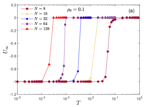
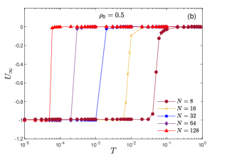
Figure 1: The temperature ($T$) dependence of long time behavior of the total energy, $U_{\infty}$, in Model I with parallel update for (a) $\rho_{0}=0.1$ and (b) $\rho_{0}=0.5$. The system transitions from a balance phase into an imbalance one, as the temperature crosses a critical value $T_{c}$ which vanishes for arbitrary large networks.

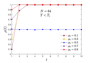
Figure 2: The time evolution of the density of positive links, $\rho(t)$, with different initial conditions of $\rho_{0}=0.1$, $0.3$, $0.5$, $0.7$, and $0.9$, for $T=10^{-4}$ ($<T_{c}$) in Model I with synchronous update rule. The network size for all plots is $N=64$.

Another important distinction between Model I and Model II is the way their dynamics is implemented numerically, i.e. synchronous vs sequential updating. In this section, we simulate Model I using synchronous (parallel) update rule instead of the originally used sequential dynamics. Therefore, given that at time $t$ energy is given by $U(t)$, for time $t+1$, we update the state of all links synchronously as follows: each link is flipped and then we calculate the total energy of the system, $U$, due to this link’s flipping. Next, by calculating $\Delta U=U-U(t)$, with probability $p$ defined in Eq. 2, this flipping is accepted or otherwise the link sign does not change. Then, we bring the system back to its previous state, and repeat the above mentioned updating rule for the next link. This is done for each individual link and finally all such resulting states are implemented in one time step, i.e. $t+1$.

Using such parallel update rule, we calculate the final total energy of the system, $U_{\infty}$, for different values of the temperature, $T$, and also for various initial positive link densities, $\rho_{0}$. We represent in Figs. 1(a) and 1(b), the values of $U_{\infty}$ versus $T$ for two initial positive link densities of $\rho_{0}=0.1$ and $\rho_{0}=0.5$, for different system sizes of $N=8$, $16$, $32$, $64$, and $128$. As can be seen, the system transitions from a balanced state ($U_{\infty}=-1$) into an imbalanced one ($U_{\infty}=0$), as it crosses a critical value. This critical value decreases as the system size increases, so that $T_{c}\to 0$ for large $N$. This indicates that the difference in the update rule is not responsible for the different scaling behavior of the critical temperature in Model I and Model II. Indeed, the difference in the behavior of the critical temperature is due to the scaling of the energy landscape.

One can see from Fig.1 that the critical temperature also depends on the initial link density $\rho_{0}$. Another important difference between Model I (sequential) and Model II (synchronous) is their balanced states dependance on the initial link density. In Model I, we found that the final state is a paradise state ($\rho=1$) for all initial link densities greater that half, and is a bipolar state ($\rho=1/2$) for all initial link densities smaller than half. On the other hand, Model II was shown to lead to a paradise state for all initial link densities except for values close to half, i.e. $\rho_{0}\approx 1/2$ where it resulted in a bipolar state. Since both balanced states are the attractor of the stochastic dynamics, one can suspect that such discrepancy is due to the update rules implemented. We therefore study Model I with synchronous dynamics in order to find the dependence of the final state on the initial conditions. The results are shown in Fig.2. As can be seen, one achieves results similar to Model II once one uses synchronous update for Model I. Our results seem to indicate that sequential update allows smooth flows in state space in order to discover the nearby attractors, while parallel update favors transitions to the paradise state, as it causes large transitions in the state space. It is important to note that previous studies have also found significant difference between various update rules within a given model Rolf1998 ; Schmoltzi1995 ; Shu2016 .

In conclusion, we have shown that the claimed discrepancy in the critical behavior of the temperature in Ref.Shojaei2019 (Model I) compared to that in Ref.Malarz2020 (Model II) can be understood in the scaling property of the energy (landscape) as a function of system size. Furthermore, we have shown that such models behave distinctly differently when updated synchronously vs. sequentially. In fact, the final balanced state strongly depends on how one updates the dynamics.

References

- (1) F. Heider, The Journal of Psychology 21, 107 (1946).
- (2) D. Cartwright and F. Harary, Psychological Review 63, 277 (1956).
- (3) T. Antal, P. L. Krapivsky, and S. Redner, Physical Review E 72, 036121 (2005).
- (4) S. A. Marvel, S. H. Strogatz, and J. M. Kleinberg, Physical Review Letters 103, 198701 (2009).
- (5) G. Facchetti, G. Iacono, and C. Altafini, Proceedings of the National Academy of Sciences 108, 20953 (2011).
- (6) S. A. Marvel, J. Kleinberg, R. D. Kleinberg, and S. H. Strogatz, Proceedings of the National Academy of Sciences 108, 1771 (2011).
- (7) R. Shojaei, P. Manshour, and A. Montakhab, Physical Review E 100, 022303 (2019).
- (8) R. J. Glauber, Journal of Mathematical Physics 4, 294 (1963)
- (9) K. Malarz and K. Kułakowski, arXiv:2009.10136 , (2020).
- (10) J. Rolf, T. Bohr, and M. H. Jensen, Physical Review E 57, R2503(R) (1998).
- (11) K. Schmoltzi, and H. G. Schuster, Physical Review E 52, 5273 (1995).
- (12) P. Shu, W. Wang, M. Tang, P. Zhao, and Y.-C. Zhang, Chaos 26, 063108(2016).