Towards Trainable Saliency Maps in Medical Imaging

Abstract

While success of Deep Learning (DL) in automated diagnosis can be transformative to the medicinal practice especially for people with little or no access to doctors, its widespread acceptability is severely limited by inherent black-box decision making and unsafe failure modes. While saliency methods attempt to tackle this problem in non-medical contexts, their apriori explanations do not transfer well to medical usecases. With this study we validate a model design element agnostic to both architecture complexity and model task, and show how introducing this element gives an inherently self-explanatory model. We compare our results with state of the art non-trainable saliency maps on RSNA Pneumonia Dataset and demonstrate a much higher localization efficacy using our adopted technique. We also compare, with a fully supervised baseline and provide a reasonable alternative to it’s high data labelling overhead. We further investigate the validity of our claims through qualitative evaluation from an expert reader.

tab:operatornames Models R-18 R-34 R-50 R-101 R-152 D-121 D-169 V-19 Baseline 98.39 98.17 98.32 98.45 97.14 96.65 97.39 98.72 Modified 98.77 98.94 98.92 98.80 98.97 97.90 98.10 98.90 Retinanet 98.81 98.16 97.08 97.88 98.25 - - - Modified 32.74 24.35 31.45 24.17 43.84 30.40 30.25 33.08 Retinanet 38.75 35.14 32.40 37.01 36.16 - - - GRAD 38.26 31.37 31.36 37.71 33.21 27.88 31.92 25.09 SG 26.05 29.21 30.41 36.27 31.55 29.76 30.34 18.55 IG 41.19 34.09 29.46 38.73 34.16 28.47 30.54 22.58 SIG 31.07 34.98 30.10 39.11 31.79 29.76 30.41 18.60 GCAM 32.83 45.91 48.66 45.71 24.67 29.57 37.27 24.69 GBP 38.26 31.37 31.36 37.71 33.21 27.88 31.92 28.27 GGCAM 44.76 39.55 39.49 45.22 32.30 34.66 37.05 32.80 Modified 48.04 46.18 48.16 48.43 50.27 42.87 45.56 54.84 Retinanet 57.55 54.99 52.91 54.56 56.13 - - -

Table 1: Classification AUC scores (top), Pointwise Detection scores (middle) and Localization Utility AUPRC scores with Retinanet baseline (bottom)

1 Introduction

Image localization is a crucial supplement to image classification especially in clinical contexts as it allows 1) comprehension of model decision 2) assessment of failure modes and, 3) identification of regions of interest (ROIs) that can guide subsequent imaging and clinical management. Approaches offering fine localization rely heavily on detailed and time consuming annotations either as bounding boxes or pixel level segmentations from clinical experts. To limit the need for large-scale annotations, methods employing Semi Supervised Learning (SSL)(Chen et al., 2019) and Weakly Supervised Learning (WSL)(Lian et al., 2019; Wang et al., 2019) have recently gained much attention from the medical imaging community. While the SSL framework augments a small pool of labeled samples with a large pool of unlabeled samples, WSL requires training with noisy or uncertain labels. Additionally, post-hoc saliency methods have long been used in a classification setup to explain classifier outputs (Mahapatra et al., 2016; Pasa et al., 2019; Bush, 2016) and as medical abnormality localizers(Amit et al., 2017; Deepak et al., 2013). However, since they are not trained end-to-end with the network, they offer limited efficacy in medical imaging applications (Arun et al., 2020). As more models are developed for routine usage by clinicians, interpretability and localizability of findings remain pivotal to building trust and acceptability in medical community.

Contribution

In this study, we adapt a previously developed WSL technique to deliver loose bounding-box localization, utilizing only image-level classification labels for pneumonia in chest radiographs. More specifically, our method automatically outputs the ROI responsible for making pneumonia prediction in the given classification model without 1) need for retraining 2) loss of classification performance 3) ground truth annotations. We further compare our method with non-trainable saliency based methods using a quantitative and qualitative set of evaluation metrics for localization success and demonstrate a failure mode assessment of the model by a radiology resident.

fig:maps

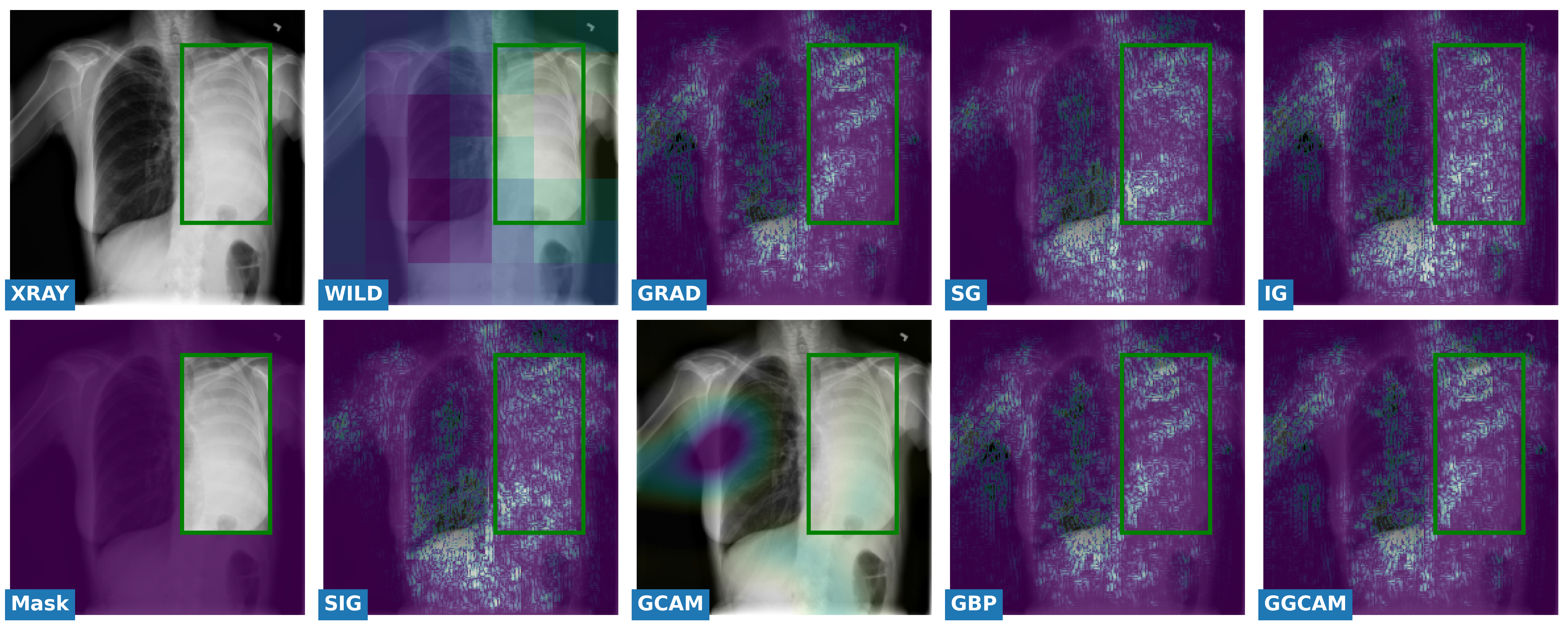
Figure 1: Respective saliency methods visualized with inverted heatmaps highlighting ROIs

2 Setup

Dataset

The dataset used for this analysis comprises of chest radiographs from the second stage of RSNA Pneumonia Detection Challenge (RSN, 2018) and contains $26,684$ scans, each labelled with one of ’Lung opacity’, ’No Lung Opacity/Not Normal’, and ’Normal’. For the purpose of this study, we excluded all ’No Lung Opacity/Not Normal’ images, so as to restrict lung opacity as a pneumonia indicator. The dataset was then split in a 80:10:10 ratio with nearly 40% positive pneumonia cases, all having bounding box annotations.

Architecture

The most commonly used convolutional neural network (CNN) architectures for classification, such as Densenet (Iandola et al., 2014), Resnet (He et al., 2015) and VGG (Simonyan and Zisserman, 2015), are primarily composed of two segments 1) Feature Network 2) Classifier Network. Of these, the former preserves spatially relevant context information, an element that is critical to the success of the WILDCAT model design (Durand et al., 2017) which we subsequently use. The latter, both here and in general, is often a fully connected network that outputs the prediction probability score.

In this technique, the given classifier network is replaced with two spatially aware pooling layers. The first layer splits the feature network output into Maps (m) * Classes (c) number of channels, which are then pooled to yield an activation map for each class, thus, forming the first part of the two valued output. These classwise maps are then fed into a spatial pooling layer which takes weighted (1:$\alpha$) average of the k highest and lowest activation pixel values to give the final prediction score.

Experiments

To validate generalizabilty of above technique, we present results over 8 different architectures and parameter counts - Resnet-18, 34, 50, 101, 152, Densenet-121, 169 and VGG-19. For comparison we also present results over 7 commonly used saliency method techniques - Gradient Explanation (GRAD), Smoothgrad (SG), Integrated Gradients (IG), Smoothgrad on Integrated Gradients (SIG), GradCAM (GCAM), Guided-backprop (GBP), and Guided GradCAM (GGCAM) along with a state of the art object detection framework, Retinanet, variants of which occupy top three positions on the original challenge leaderboard (RSN, 2018). Each model presented has undergone multiple runs with different seed values, early stopping, minimum data pre-processing and an extensive hyperparameter search (Appendix B).

3 Results

Classification

As shown in Table 1 (top block), modified architectures always outperform baseline for each of the model types considered, thus, verifying that we not only maintain classification performances but are better by 0.5-1%. We also find the best results are consistently obtained at low k values, implying the model focuses only on specific areas (ROIs) in the modified architecture to make a successful prediction.

Pointwise Detection

For detection evaluation by our models, we follow the pointwise detection metric adopted by the Wildcat (Durand et al., 2017) paper. This metric captures the quality of detection without penalizing the lack of an appropriately sized bounding box. Each classwise map (s*s) is extrapolated to match the size of the original input image (S*S) resulting in fixed size bounding box (d*d, where d = S/s). Table 1 (middle block) reports mean Average Precision scores, with modified ResNet-152 performing better by a 5% margin than the best performing Retinanet network, our fully supervised detection baseline.

Localization Utility

To improve interpretabilty and reliability of classification tasks, it is imperative to provide clinicians with meaningful visualizations of model rationale behind a prediction. We thus aim to provide high quality visualizations with classwise maps. The extrapolated map can be viewed in juxtaposition with the original radiograph (first row, second column in LABEL:fig:maps) to highlight abnormal regions which are suspected pneumonia ROIs. To justify their efficacy, we compare classwise map, saliency methods’ map and retinanet box output map with ground truth annotation mask, and calculate a simple similarity score (Appendix B) between former and latter to provide results. Classwise maps are clearly superior to the saliency maps. The best performing saliency method, GGCAM, is still worse off by 10% on average than modified architecture and the best performing model type, VGG19, has comparable performance to average performance of fully supervised baseline.

Reader Study

fig:reader

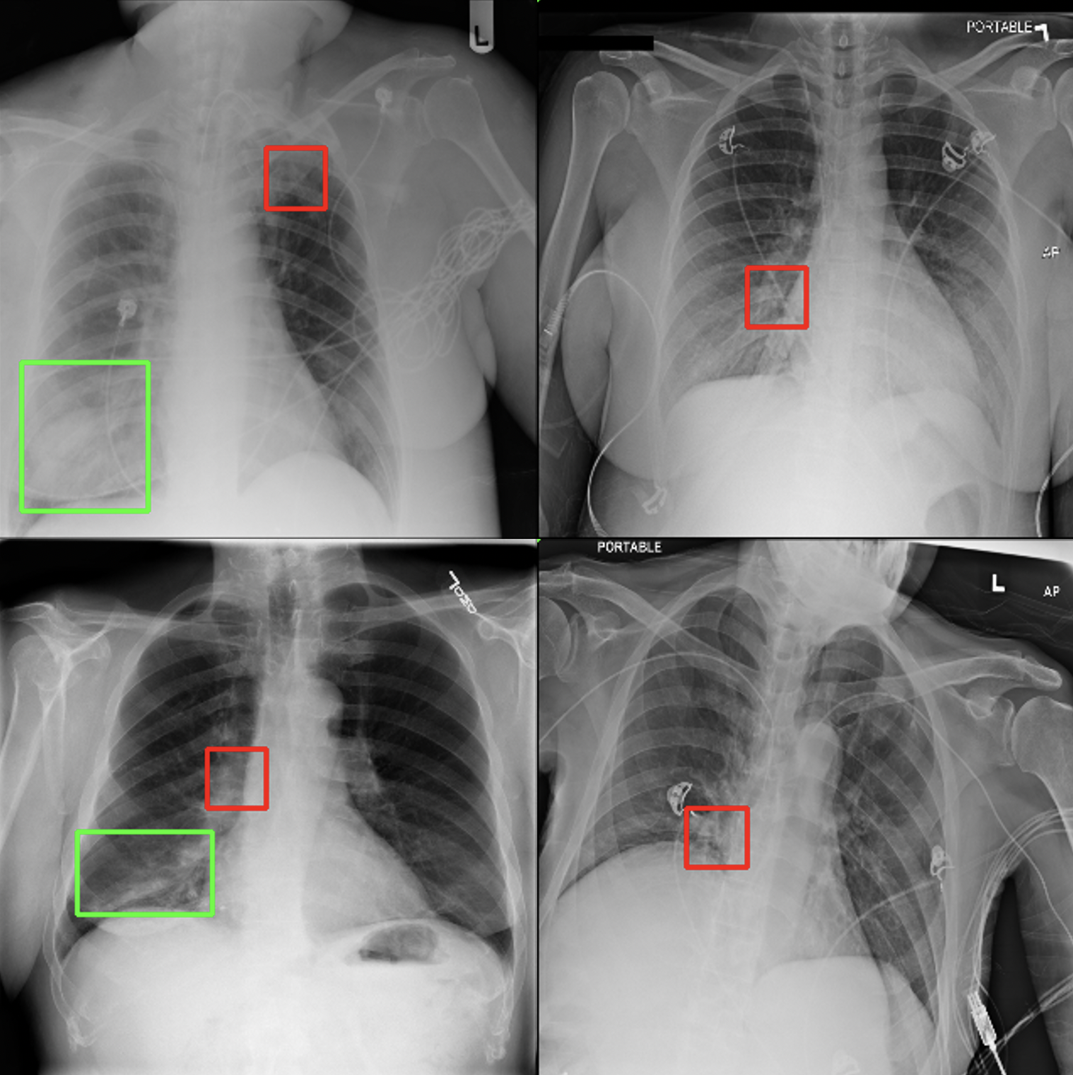
Figure 2: FN (Left) and FP (Right)

A senior diagnostic radiology resident inspected model failure cases. The cases were divided into classification false positives (FP) and true positives but with no predicted box overlap with ground truth bounding box (FN). As seen in Fig LABEL:fig:reader, for FP cases, most showed localization to either the hilum of lung or a clavicle projecting over lung apex. Both sites represent sites of increased density that the model mistook for pneumonia. For FN cases, we similarly find that the predicted bounding box tends to localize to lung hilum (and to lesser extent the clavicle projecting over lung apex), instead of actual lung pathology of interest. Overall model tends to incorrectly identify normal opacities of the hilum and clavicle as pneumonia. These are challenging features for the model to learn, as many diverse pathologies occur at the hilum and lung apices but even here, clinical failure can be avoided by quick confirmation with the predicted box.

4 Conclusion

In this study, we validate a WSL pipeline for interpretation and abnormality localization for pneumonia classification models using only image-level labels. Our approach is trained end-to-end with classification labels, improving base performance and outperforming saliency map methods which are commonly used in medical literature for model interpretation and localization. Our results have implications for the clinical deployment of deep learning models, increasing their utility and explainability for clinicians. This may facilitate their trust in the models and expedite integration into the clinical workflow.

Appendix A Training Details

For both the baseline classification model and the modified WILDCAT model, a batch size of 64 images, binary cross entropy loss function, Adam optimizer and early stopping with patience of 10 epochs on loss change was used across models. Best baseline model across mutiple learning rates and best WILDCAT model across mutiple learning rates, k, $\alpha$ and m parameters was used to present results. Both localization utility and pointwise detection results are presented over best performing classification models, mimicking real world deployment where lack of ground truth annotations make optimizing over localization performance intractable. Overall, multiple runs with different seeds, amounting to over 1200+ trained models were analysed to effectively validate statistical reliability of each presented result.

Appendix B Metric Explanations

Pointwise Detection

The metric identifies a successful localization as one where the center point of the predicted bounding box lies inside the ground truth annotation box. Similar to the standard mean Average Precision (mAP) calculation for object detection, the True positives defined here, should satisfy both high confidence score and the localization criteria given above. False positives and False negatives for the same can be defined congruently.

Localization Utility

The metric estimates the area under the precision recall curve (AUPRC) by treating, for single image, the binary array obtained from annotation mask as the ground truth labels and, the continuous, normalized array obtained from saliency maps as the predicted scores. From here, the calculated AUPRC score for each image is averaged to give the final localization utility result. Thus, the metric clearly captures extent of similarity between given annotation mask and the saliency map. In the figure fig:auprc given below, we present a sample saliency map and it’s corresponding precision recall curve. Further, for Retinanet detection baseline, the map is obtained by allocating each pixel the value of the highest scoring box that covers it.

fig:auprc

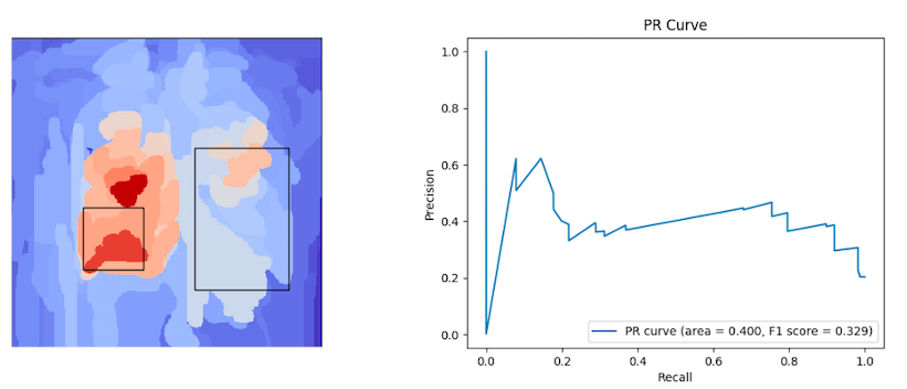
Figure 3: Saliency map and its PR Curve

References

- RSN (2018) Rsna pneumonia detection challenge. https://www.kaggle.com/c/rsna-pneumonia-detection-challenge/overview, 2018.
- Amit et al. (2017) Guy Amit, Omer Hadad, Sharon Alpert, Tal Tlusty, Yaniv Gur, Rami Ben-Ari, and Sharbell Hashoul. Hybrid mass detection in breast mri combining unsupervised saliency analysis and deep learning. In International conference on medical image computing and computer-assisted intervention, pages 594–602. Springer, 2017.
- Arun et al. (2020) Nishanth Arun, Nathan Gaw, Praveer Singh, Ken Chang, Mehak Aggarwal, Bryan Chen, Katharina Hoebel, Sharut Gupta, Jay Patel, Mishka Gidwani, Julius Adebayo, Matthew D. Li, and Jayashree Kalpathy-Cramer. Assessing the (un)trustworthiness of saliency maps for localizing abnormalities in medical imaging, 2020.
- Bush (2016) Isabel Bush. Lung nodule detection and classification. vol, 20:196–209, 2016.
- Chen et al. (2019) Shuai Chen, Gerda Bortsova, Antonio García-Uceda Juárez, Gijs van Tulder, and Marleen de Bruijne. Multi-task attention-based semi-supervised learning for medical image segmentation. In International Conference on Medical Image Computing and Computer-Assisted Intervention, pages 457–465. Springer, 2019.
- Deepak et al. (2013) K Sai Deepak, Arunava Chakravarty, Jayanthi Sivaswamy, et al. Visual saliency based bright lesion detection and discrimination in retinal images. In 2013 IEEE 10th International Symposium on Biomedical Imaging, pages 1436–1439. IEEE, 2013.
- Durand et al. (2017) Thibaut Durand, Taylor Mordan, Nicolas Thome, and Matthieu Cord. Wildcat: Weakly supervised learning of deep convnets for image classification, pointwise localization and segmentation. In Proceedings of the IEEE conference on computer vision and pattern recognition, pages 642–651, 2017.
- He et al. (2015) Kaiming He, Xiangyu Zhang, Shaoqing Ren, and Jian Sun. Deep residual learning for image recognition. CoRR, abs/1512.03385, 2015. URL http://arxiv.org/abs/1512.03385.
- Iandola et al. (2014) Forrest Iandola, Matt Moskewicz, Sergey Karayev, Ross Girshick, Trevor Darrell, and Kurt Keutzer. Densenet: Implementing efficient convnet descriptor pyramids. arXiv preprint arXiv:1404.1869, 2014.
- Lian et al. (2019) Chunfeng Lian, Mingxia Liu, Li Wang, and Dinggang Shen. End-to-end dementia status prediction from brain mri using multi-task weakly-supervised attention network. In International Conference on Medical Image Computing and Computer-Assisted Intervention, pages 158–167. Springer, 2019.
- Mahapatra et al. (2016) Dwarikanath Mahapatra, Pallab K Roy, Suman Sedai, and Rahil Garnavi. Retinal image quality classification using saliency maps and cnns. In International Workshop on Machine Learning in Medical Imaging, pages 172–179. Springer, 2016.
- Pasa et al. (2019) F Pasa, V Golkov, F Pfeiffer, D Cremers, and D Pfeiffer. Efficient deep network architectures for fast chest x-ray tuberculosis screening and visualization. Scientific reports, 9(1):1–9, 2019.
- Simonyan and Zisserman (2015) Karen Simonyan and Andrew Zisserman. Very deep convolutional networks for large-scale image recognition, 2015.
- Wang et al. (2019) Yirui Wang, Le Lu, Chi-Tung Cheng, Dakai Jin, Adam P Harrison, Jing Xiao, Chien-Hung Liao, and Shun Miao. Weakly supervised universal fracture detection in pelvic x-rays. In International Conference on Medical Image Computing and Computer-Assisted Intervention, pages 459–467. Springer, 2019.