Deep-RLS: A Model-Inspired Deep Learning Approach to Nonlinear PCA

Abstract

In this work, we consider the application of model-based deep learning in nonlinear principal component analysis (PCA). Inspired by the deep unfolding methodology, we propose a task-based deep learning approach, referred to as Deep-RLS, that unfolds the iterations of the well-known recursive least squares (RLS) algorithm into the layers of a deep neural network in order to perform nonlinear PCA. In particular, we formulate the nonlinear PCA for the blind source separation (BSS) problem and show through numerical analysis that Deep-RLS results in a significant improvement in the accuracy of recovering the source signals in BSS when compared to the traditional RLS algorithm.

Index Terms—  Deep learning, deep unfolding, blind source separation, principal component analysis.

1 Introduction

Principal component analysis (PCA) is a linear orthogonal transformation that determines the eigenvectors or the basis vectors associated with the covariance matrix of the observed data. The output of the standard PCA is the projection of the data onto the obtained basis vectors, resulting in principal components which are mutually uncorrelated.

As a related problem, blind source separation (BSS)  [1] aims to recover statistically independent source signals from linear mixtures whose composition gains are unknown. In fact, the only knowledge about the source signals to be recovered in BSS is their independence. This is a stronger assumption than what one requires for PCA, i.e. uncorrelated signal sources. This suggest that performing PCA on such a mixture of signals may not successfully separate them, and that higher order statistics is required to verify and ensure the independence of the source signals.

In light of the above, the notion of nonlinear correlation was introduced to verify the independence of signals more effectively [2]. It was also shown that an extension of PCA to the nonlinear domain (known as nonlinear PCA) can separate independent components of the mixture [2]. In [1], an objective function targeting the fourth-order moments of the distribution of the recovered signals is suggested. It is proved that minimizing this objective function can obtain the independent source signals under the assumption that all sources have negative kurtosis, i.e. they are sub-Gaussian. Minimizing such an objective functions introduces nonlinearities in the signal recovery and the learning process.

In this paper, we propose a deep learning approach to nonlinear PCA that relies on the unfolding of an iterative algorithm into the layers of a deep neural network in order to perform the nonlinear PCA task; i.e. to estimate the source signals for BSS. In particular, we use the classical recursive least squares [3] to construct the network structure and to iteratively estimate the source signals. We experimentally verify the performance of our algorithm and compare it with the traditional RLS algorithm.

2 Problem Formulation

2.1 Nonlinear PCA for Blind Source Separation

We begin by considering the longstanding BSS problem in which $m$ statistically independent signals are linearly mixed to yield $l$ possibly noisy combinations

$${\mathbf{x}(t)}={\mathbf{A}}{\mathbf{s}(t)}+{\mathbf{n}(t)}.$$ (1)

Let ${\mathbf{x}(t)}=[x_{1}(t),\ldots,x_{l}(t)]^{T}$ denote the $l-$dimensional data vector made up of the mixture at time $t$ that is exposed to an additive noise ${\mathbf{n}(t)}$. Given no knowledge of the mixing matrix ${\mathbf{A}}\in\mathds{R}^{m\times l}$, the goal is to recover the original source signal vector ${\mathbf{s}(t)}=[s_{1}(t),\ldots,s_{m}(t)]^{T}$ from the mixture.

A seminal work in this context is [1] which suggests tuning and updating a separating matrix ${\mathbf{W}}\in\mathds{R}^{l\times m}$ until the output

$${\mathbf{y}(t)}={\mathbf{W}}^{T}{\mathbf{x}(t)},$$ (2)

where ${\mathbf{y}(t)}=[y_{1}(t),\ldots,y_{m}(t)]^{T}$, is as close as possible to the source signal vector of interest ${\mathbf{s}(t)}$. Assuming there exists a larger number of sensors than the source signals, i.e. $l\geq m$, we can draw an analogy between the BSS problem and the task of PCA. In a sense, we are aiming to represent the random vector ${\mathbf{x}(t)}$ in a lower dimensional orthonormal subspace, represented by the columns of ${\mathbf{W}}$, as the orthonormal basis vectors. By this analogy, both BSS and PCA problems can be reduced to minimizing an objective function of the from:

$$\mathcal{L}({\mathbf{W}})=\mathbb{E}\left\{\|{\mathbf{x}(t)}-{\mathbf{W}}({\mathbf{W}}^{T}{\mathbf{x}(t)})\|_{2}^{2}\right\}.$$ (3)

Assuming that ${\mathbf{x}(t)}$ is a zero-mean vector, it can be shown that the solution to the above optimization problem is a matrix ${\mathbf{W}}$ whose columns are the $m$ dominant eigenvectors of the data covariance matrix $\mathbf{C_{x}}(t)=\mathbb{E}\left\{{\mathbf{x}(t)}{\mathbf{x}(t)}^{T}\right\}$ [2]. Therefore, the principal components or the recovered source signals are mutually uncorrelated. As previously discussed in Section 1, having uncorrelated data is not a sufficient condition to achieve separation. In other words, the solutions to PCA and BSS do not coincide unless we address the higher order statistics of the output signal ${\mathbf{y}(t)}$. By introducing nonlinearity into (3), we will implicitly target higher order statistics of the signal [2]. This nonlinear PCA, which is an extension of the conventional PCA, is made possible by considering the signal recovery objective:

$$\mathcal{L}({\mathbf{W}})=\mathbb{E}\left\{\|{\mathbf{x}(t)}-{\mathbf{W}}\mathbf{g}({\mathbf{W}}^{T}{\mathbf{x}(t)})\}\|_{2}^{2}\right\},$$ (4)

where $\mathbf{g}(\cdot)$ denotes an odd non-linear function applied element-wise on the vector argument. We invite the interested readers to find a proof of the connection between (4) and higher order statistics of the source singals ${\mathbf{s}(t)}$ in [4].

While PCA is a fairly standardized technique, nonlinear or robust PCA formulations based on (4) tend to be multi-modal with several local optima—so they can be run from various initial points and possibly lead to different “solutions” [5]. In [3], a recursive least squares algorithm for subspace estimation is proposed, which is further extended to the nonlinear PCA in [6] for solving the BSS problem. We consider the algorithm in [6] as a baseline for developing our deep unfolded framework for nonlinear PCA.

2.2 Recursive Least Squares for Nonlinear PCA

We consider a real-time and adaptive scenario in which upon arrival of new data ${\mathbf{x}(t)}$, the subspace of signal at time instant $t$ is recursively updated from the subspace at time $t-1$ and the new sample ${\mathbf{x}(t)}$ [3]. The separating matrix ${\mathbf{W}}$ introduced in Section 2.1 is therefore replaced by ${\mathbf{W}(t)}$ and updated at each time instant $t$. The adaptive algorithm chosen for this task is the well-known recursive least squares (RLS) [7].

In the linear case, by replacing the expectation in (3) with a weighted sum, we can attenuate the impact of the older samples, which is reasonable, for instance whenever one deals with a time-varying environment. In this way, one can make sure the distant past will be forgotten and the resulting algorithm for minimizing (3) can effectively track the statistical variations of the observed data. By replacing ${\mathbf{y}(t)}={\mathbf{W}(t)}^{T}{\mathbf{x}(t)}$ and using an exponential weighting (governed by a forgetting factor), the loss function in (3) boils down to:

$$\mathcal{L}({\mathbf{W}(t)})=\sum_{i=1}^{t}\beta^{t-i}||{\mathbf{x}(t)}-{\mathbf{W}(t)}{\mathbf{y}(t)}||^{2},$$ (5)

with the forgetting factor $\beta$ satisfying $0\ll\beta\leq 1$. Note that $\beta=1$ yields the ordinary method of least squares in which all samples are weighed equally while choosing relatively small $\beta$ makes our estimation rather instantaneous, thus neglecting the past. Therefore, $\beta$ is usually chosen to be less than one, but also rather close to one for smooth tracking and filtering.

Note that one may write the gradient of the loss function in (5) in its compact form as

$$\nabla_{{\mathbf{W}}}\mathcal{L}({\mathbf{W}})=-2\mathbf{C_{xy}}(t)+2\mathbf{C_{y}}(t){\mathbf{W}},$$ (6)

where $\mathbf{C_{y}}(t)$ and $\mathbf{C_{xy}}(t)$ are the auto-correlation matrix of ${\mathbf{y}(t)}$,

$$\mathbf{C_{y}}(t)=\sum_{i=1}^{t}\beta^{t-i}\mathbf{y}(i)\mathbf{y}(i)^{T}=\beta\mathbf{C_{y}}(t-1)+{\mathbf{y}(t)}{\mathbf{y}(t)}^{T},$$ (7)

and the cross-correlation matrix of ${\mathbf{x}(t)}$ and ${\mathbf{y}(t)}$,

$$\mathbf{C_{xy}}(t)=\sum_{i=1}^{t}\beta^{t-i}\mathbf{x}(i)\mathbf{y}(i)^{T}=\beta\mathbf{C_{xy}}(t-1)+{\mathbf{x}(t)}{\mathbf{y}(t)}^{T},$$ (8)

at the time instance $t$, respectively. Setting the gradient (6) to zero will result in the close-form separating matrix,

$${\mathbf{W}(t)}=\mathbf{C_{y}}^{-1}(t)\mathbf{C_{xy}}(t).$$ (9)

1:Initialize $W(0)$ and $P(0)$

2:for $t=0,1,\ldots,T$ do

      

3: ${\mathbf{y}(t)}=\mathbf{W}^{T}(t-1){\mathbf{x}(t)}$

4: ${\mathbf{h}(t)}=\mathbf{P}(t-1){\mathbf{y}(t)}$

5: ${\mathbf{f}(t)}=\frac{{\mathbf{h}(t)}}{\beta+\mathbf{y}(t)^{T}{\mathbf{h}(t)}}$

6: ${\mathbf{P}(t)}=\beta^{-1}[\mathbf{P}(t-1)-{\mathbf{f}(t)}\mathbf{h}(t)^{T}]$

7: ${\mathbf{e}(t)}={\mathbf{x}(t)}-\mathbf{W}(t-1){\mathbf{y}(t)}$

8: ${\mathbf{W}(t)}=\mathbf{W}(t-1)+{\mathbf{e}(t)}\mathbf{f}(t)^{T}$

Algorithm 1 RLS Algorithm for Performing PCA

A recursive computation of ${\mathbf{W}(t)}$ can be achieved using the RLS algorithm [7]. In RLS, the matrix inversion lemma enables a recursive computation of ${\mathbf{P}(t)}=\mathbf{C_{y}}^{-1}(t)$; see the derivations in Appendix. At each iteration of the RLS algorithm, ${\mathbf{P}(t)}$ is recursively computed as

$${\mathbf{P}(t)}=\beta^{-1}\mathbf{P}(t-1)-\frac{\beta^{-2}\mathbf{P}(t-1){\mathbf{y}(t)}{\mathbf{y}(t)}^{T}\mathbf{P}(t-1)}{1+\beta^{-1}{\mathbf{y}(t)}^{T}\mathbf{P}(t-1){\mathbf{y}(t)}}.$$ (10)

Consequently, the RLS algorithm provides the estimate ${\mathbf{y}(t)}$ of the source signals. The steps of the RLS algorithm are summarized in Algorithm 1.

It appears that extending the application of RLS to the nonlinear PCA loss function in (4) is rather straightforward. To accomplish this task, solely step 3 of Algorithm 1 should be modified to ${\mathbf{y}(t)}=g({\mathbf{W}}^{T}(t-1){\mathbf{x}(t)})$ in order to meet the nonlinear PCA criterion [3]. In the following, we unfold the iterations of the modified Algorithm 1, for nonlinear PCA onto the layers of a deep neural network where each layer resembles one iteration of the RLS algorithm. Interestingly, one can fix the complexity budget of the inference framework via fixing the number of layers, and apply the RLS-based proposed method to yield an estimation of the source signals.

3 Deep Unfolded RLS for Nonlinear PCA

Deep neural networks (DNN) are one of the most studied approaches in machine learning owing to their significant potential. They are usually used as a black-box without incorporating any knowledge of the system model. Moreover, they are not always practical to use as they require a large amount of training data and considerable computational resources. Hershey, et al., in [8], introduced a technique referred to as deep unfolding or unrolling in order to enable the community to address the mentioned issues with DNNs. The deep unfolding technique lays the ground for bridging the gap between well-established iterative signal processing algorithms that are model-based in nature and deep neural networks that are purely data-driven. Specifically, in deep unfolding, each layer of the DNN is designed to resemble one iteration of the original algorithm of interest. Passing the signals through such a deep network is in essence similar to executing the iterative algorithm a finite number of times, determined by the number of layers. In addition, the algorithm parameters (such as the model parameters and forgetting parameter in the RLS algorithm) will be reflected in the parameters and weights of the constructed DNN. The data-driven nature of the emerging deep network thus enables improvements over the original algorithm. Note that the constructed network may be trained using back-propagation, resulting in model parameters that are learned from the real-world training datasets. In this way, the trained network can be naturally interpreted as a parameter optimized algorithm, effectively overcoming the lack of interpretability in most conventional neural networks [9]. In comparison with a generic DNN, the unfolded network has much fewer parameters and therefore requires a more modest size of training data and computational resources. The deep unfolding technique has been deployed for many signal processing problems and has dramatically improved the convergence rate of the state-of-the-art model-based iterative algorithms; see, e.g., [10, 11, 12] and the references therein.

Due to the promises of deep unfolding in addressing the shortcomings of both generic deep learning methods and model-based signal processing algorithms, we have been motivated to deploy this technique to improve the recursive least squares solution for nonlinear PCA. As shown in [6], when applied to a linear mixture of source signals (i.e., the BSS problem), the RLS algorithm usually approximates the true source signals well and successfully separates them. However, the number of iterations needed to converge may vary greatly depending on the initial values and the forgetting parameter $\beta$. Inspired by the deep unfolding technique, we introduce Deep-RLS, our deep learning-based framework which is designed based on the modified iterations of the algorithm 1. More precisely, the dynamics of the $k$-th layer of Deep-RLS are given as:

$$\mathbf{y}(k) =\mathbf{g}(\mathbf{H}_{k}\mathbf{W}^{T}(k-1)\mathbf{x}(k)+\mathbf{b}_{k}),$$ (11a)

$$\mathbf{h}(k) =\mathbf{P}(k-1)\mathbf{y}(k),$$ (11b)

$$\mathbf{f}(k) =\frac{\mathbf{h}(k)}{\mathbf{\omega}_{k}+\mathbf{y}(k)^{T}\mathbf{h}(k)},$$ (11c)

$$\mathbf{P}(k) =\omega_{k}^{-1}[\mathbf{P}(k-1)-\mathbf{f}(k)\mathbf{h}(k)^{T}],$$ (11d)

$$\mathbf{e}(k) =\mathbf{x}(k)-\mathbf{H}_{k}{\mathbf{W}}(k-1)\mathbf{y}(k),$$ (11e)

$${\mathbf{W}}(k) =\mathbf{H}_{k}{\mathbf{W}}(k-1)+\mathbf{e}(k)\mathbf{f}(k)^{T},$$ (11f)

where $\mathbf{x}(k)$ is the data vector at the time instance $k$, $\mathbf{g}(.)$ is a nonlinear activation function which can be chosen by considering the distribution of the source signals, $\omega_{k}\in\mathds{R}$ represents the trainable forgetting parameter, and $\mathbf{H}_{k}\in\mathds{R}^{m\times m}$ and $\mathbf{b}_{k}\in\mathds{R}^{m}$ denotes the set of trainable weights and biases of the $k$-th layer, respectively. In [5], it was shown that for source signals ${\mathbf{s}(t)}$ with sub-Gaussian distribution, $\mathbf{g}(\mathbf{x})=tanh(\mathbf{x})$ results in convergence of the nonlinear PCA to the true source signals.

1:Initialize ${\mathbf{W}}(0)$ and $\mathbf{P}(0)$

2:for $epoch=1,\ldots,N$ do

      for $k=1,\ldots,T$ do

            Feed $\mathbf{x}(k)$ to $k$-th layer of the network
Apply the recursion in (11)

      

      Compute the loss function (13)

      Use backpropagation to update $\{\Gamma_{k}\}_{k=1}^{T}$

Algorithm 2 Training Procedure for Deep-RLS

Given $T$ samples of the data vector ${\mathbf{x}(t)}$, our goal is to optimize the parameters $\{\Gamma_{k}\}_{k=1}^{T}$ of the DNN, where

$$\Gamma_{k}=\{\mathbf{H}_{k},\mathbf{\omega}_{k},\mathbf{b}_{k}\}.$$ (12)

The output of the $k$-th layer is an approximation of the source signals at the time instance $k$. For training of the proposed Deep-RLS network, we consider cumulative MSE loss of the layers. In designing the training procedure, one needs to consider the constraint that the forgetting parameter must satisfy $0<\beta\leq 1$. Hence, in order to impose such a constraint, one can regularize the loss function ensuring that the network chooses proper weights $\{\omega_{k}\}_{k=1}^{T}$ corresponding to a feasible forgetting parameter at each layer [13]. Accordingly, we define the loss function used for the training of the proposed architecture as follows:

$$\begin{split}\mathcal{L}({\mathbf{W}}(k))&=\underbrace{\sum_{k=1}^{T}||\mathbf{x}(k)-{\mathbf{W}}(k)\mathbf{y}(k)||^{2}}_{\text{accumulated loss of all layers}}+\\ &\underbrace{\lambda\sum_{k=1}^{T}\mathrm{ReLU}(-\mathbf{\omega}_{k})+\lambda\sum_{k=1}^{T}\mathrm{ReLU}(\mathbf{\omega}_{k}-1)}_{\text{regularization term for the forgetting parameter}},\end{split}$$ (13)

where $\mathrm{ReLU}(\cdot)$ is the well-known Rectifier Linear Unit function extensively used in the deep learning literature. We have presented the employed training process in Algorithm 2.

4 Numerical Result

In this section, we demonstrate the performance of the proposed Deep-RLS for nonlinear PCA in the case of blind source separation. The proposed framework was implemented using the PytTorch library [14] and the Adam stochastic optimizer [15] with a learning rate of $10^{-3}$ for training purposes.

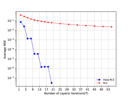
Fig. 1: The average MSE of recovering $m=2$ source signals using the Deep-RLS network vs. the number of layers/iterations $T$ when trained for $N=50$ epochs. The proposed method significantly outperforms the RLS algorithm with $\beta=0.99$.

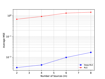
Fig. 2: The performance of Deep-RLS and the the traditional RLS algorithm when applied to the recovery of a growing number of source signals.

The training was performed based on the data generated via the following model. For the time interval $t=0,1,...,T$, each element of the vector $s(t)$ is to be generated from a sub-Gaussian distribution. For data generation purposes, we have assumed the source signals to be i.i.d. and uniformly distributed, i.e., $s(t)\sim\mathcal{U}(0,1)$. The mixing matrix $\mathbf{A}$ is assumed to be fixed and generated once according to a Normal distribution, i.e., $\mathbf{A}\sim\mathcal{N}(\mathbf{0},\mathbf{I})$. We performed the training of the proposed Deep-RLS using the batch learning process with a batch size of 40 and trained the network for $N=50$ epochs. A training set of size $10^{3}$ and test set of size $10^{2}$ was chosen. We used the average of the mean-square-error (MSE), $\mathrm{MSE}=(1/T)\sum_{k=1}^{T}||\mathbf{s}(k)-\mathbf{y}(k)||^{2}_{2}$, as the performance metric. In Fig. 1, the performance of RLS implemented with $\beta=0.99$ at different number of iterations is compared with the Deep-RLS network trained with the same number of layers. It can be observed that the average MSE obtained using the proposed architecture is much lower than RLS, even with fewer number of layers/iterations. Fig. 2 demonstrates the performance of the proposed Deep-RLS network and the original RLS algorithm in terms of the average MSE for a growing number of source signals $m$. It can be observed from both Figs. 1 and 2 that the proposed method achieves a far superior performance than that of the original RLS algorithm.

5 Conclusion

We considered the application of model-based machine learning, and specifically the deep unfolding technique, for nonlinear PCA. A deep network based on the well-known RLS algorithm, which we call Deep-RLS, was proposed that outperforms its traditional model-based counterparts.

Appendix A Appendix: The RLS Recursive Formula

Let $\mathbf{A}$, $\mathbf{B}$, and $\mathbf{D}$ be positive definite matrices so that $\mathbf{A}=\mathbf{B}^{-1}+\mathbf{cD}^{-1}\mathbf{c}^{T}.$ Using the matrix inversion lemma, the inverse of $\mathbf{A}$ can be expressed as

$$\mathbf{A}^{-1}=\mathbf{B}-\mathbf{Bc}(\mathbf{D}+\mathbf{c}^{T}\mathbf{Bc})^{-1}\mathbf{c}^{T}\mathbf{B}.$$ (14)

Now, assuming that the auto-correlation matrix $\mathbf{C_{y}}(t)$ is positive definite (and thus nonsingular), by choosing $\mathbf{A=C_{y}}(t)$, $\mathbf{B}^{-1}=\beta\mathbf{C_{y}}(t-1)$,$\mathbf{c}={\mathbf{y}(t)},\mathbf{D}^{-1}=1$, one can compute ${\mathbf{P}(t)}=\mathbf{C_{y}}^{-1}(t)$ as proposed in (10).

References

- [1] J-F Cardoso and Beate H Laheld, “Equivariant adaptive source separation,” IEEE Transactions on signal processing, vol. 44, no. 12, pp. 3017–3030, 1996.
- [2] João Marcos Travassos Romano, Romis Attux, Charles Casimiro Cavalcante, and Ricardo Suyama, Unsupervised signal processing: channel equalization and source separation, CRC Press, 2018.
- [3] Bin Yang, “Projection approximation subspace tracking,” IEEE Transactions on Signal processing, vol. 43, no. 1, pp. 95–107, 1995.
- [4] Petteri Pajunen and Juha Karhunen, “Least-squares methods for blind source separation based on nonlinear PCA,” International Journal of Neural Systems, vol. 8, no. 05n06, pp. 601–612, 1997.
- [5] Juha Karhunen, Erkki Oja, Liuyue Wang, Ricardo Vigario, and Jyrki Joutsensalo, “A class of neural networks for independent component analysis,” IEEE Transactions on neural networks, vol. 8, no. 3, pp. 486–504, 1997.
- [6] Juha Karhunen and Petteri Pajunen, “Blind source separation using least-squares type adaptive algorithms,” in 1997 IEEE International Conference on Acoustics, Speech, and Signal Processing. IEEE, 1997, vol. 4, pp. 3361–3364.
- [7] S. Haykin and S.S. Haykin, Adaptive Filter Theory, Pearson, 2014.
- [8] John R Hershey, Jonathan Le Roux, and Felix Weninger, “Deep unfolding: Model-based inspiration of novel deep architectures,” arXiv preprint arXiv:1409.2574, 2014.
- [9] Vishal Monga, Yuelong Li, and Yonina C Eldar, “Algorithm unrolling: Interpretable, efficient deep learning for signal and image processing,” arXiv preprint arXiv:1912.10557, 2019.
- [10] Shahin Khobahi, Naveed Naimipour, Mojtaba Soltanalian, and Yonina C Eldar, “Deep signal recovery with one-bit quantization,” in ICASSP 2019-2019 IEEE International Conference on Acoustics, Speech and Signal Processing (ICASSP). IEEE, 2019, pp. 2987–2991.
- [11] Shahin Khobahi, Arindam Bose, and Mojtaba Soltanalian, “Deep radar waveform design for efficient automotive radar sensing,” in 2020 IEEE 11th Sensor Array and Multichannel Signal Processing Workshop (SAM). IEEE, 2020, pp. 1–5.
- [12] Oren Solomon, Regev Cohen, Yi Zhang, Yi Yang, Qiong He, Jianwen Luo, Ruud JG van Sloun, and Yonina C Eldar, “Deep unfolded robust PCA with application to clutter suppression in ultrasound,” IEEE transactions on medical imaging, vol. 39, no. 4, pp. 1051–1063, 2019.
- [13] Shahin Khobahi and Mojtaba Soltanalian, “Model-aware deep architectures for one-bit compressive variational autoencoding,” arXiv preprint arXiv:1911.12410, 2019.
- [14] Adam Paszke, Sam Gross, Francisco Massa, Adam Lerer, James Bradbury, Gregory Chanan, Trevor Killeen, Zeming Lin, Natalia Gimelshein, Luca Antiga, Alban Desmaison, Andreas Kopf, Edward Yang, Zachary DeVito, Martin Raison, Alykhan Tejani, Sasank Chilamkurthy, Benoit Steiner, Lu Fang, Junjie Bai, and Soumith Chintala, “Pytorch: An imperative style, high-performance deep learning library,” in Advances in Neural Information Processing Systems 32, H. Wallach, H. Larochelle, A. Beygelzimer, F. d'Alché-Buc, E. Fox, and R. Garnett, Eds., pp. 8024–8035. Curran Associates, Inc., 2019.
- [15] Diederik P Kingma and Jimmy Ba, “Adam: A method for stochastic optimization,” arXiv preprint arXiv:1412.6980, 2014.