Solutions of the tt*-Toda Equations and Quantum Cohomology of Flag Manifolds

Abstract.

We relate the quantum cohomology of minuscule flag manifolds to the tt*-Toda equations, a special case of the topological-antitopological fusion equations which were introduced by Cecotti and Vafa in their study of supersymmetric quantum field theories. To do this, we combine the Lie-theoretic treatment of the tt*-Toda equations of Guest-Ho with the Lie-theoretic description of the quantum cohomology of minuscule flag manifolds from Chaput-Manivel-Perrin and Golyshev-Manivel.

1. Introduction

It is well known that solutions of the 2-dimensional Toda equations correspond to primitive harmonic maps into flag manifolds. The tt*-Toda equations provide a special case of the Toda equations; here the harmonic maps can be regarded as generalizations of variations of Hodge structure, or VHS. Certain special solutions illustrate the mirror symmetry phenomenon: For example, according to Cecotti and Vafa [CV], the generalized VHS for a solution may correspond to the quantum (orbifold) cohomology of a certain Kähler manifold.
To be more precise, there are three aspects of this result. First it is necessary to establish a bijective correspondence between global solutions on $\mathbb{C}^{*}=\mathbb{C}-\{0\}$ and their “holomorphic data”. Second, this holomorphic data has to be identified with a flat connection of the type used by Dubrovin in the theory of Frobenius manifolds - we call it the Dubrovin connection. Finally, for certain specific solutions, this has to be identified with the Dubrovin connection associated to the (small) quantum cohomology of a specific Kähler manifold. Guest, Its and Lin have investigated all three aspects in the case of the Lie group type $A_{n}$ [GIL].
In [GH] the tt*-Toda equations are described for general complex simple Lie algebras. Guest and Ho obtained a correspondence between solutions and the fundamental Weyl alcove. It is expected (but not yet proved beyond the $A_{n}$ case) that this gives a bijective correspondence between global solutions and points of (a subset of) the fundamental Weyl alcove.
This paper is a contribution to the second and third aspects of the generalization of [GIL] to the case of general complex simple Lie algebras. That is, we shall establish a correspondence between the holomorphic data of certain specific solutions of the tt*-Toda equations and the Dubrovin connections of minuscule flag manifolds, based on the Lie-theoretic approach of [GH]. Minuscule flag manifolds are the projectivized weight orbits of minuscule weights (see [CMP]).
The quantum cohomology of flag manifolds has been the subject of many articles, especially from the point of view of quantum Schubert calculus. For Lie-theoretic treatments we mention in particular [FW]. The minuscule case has been studied in detail in [CMP].
Golyshev and Manivel [GM] described the quantum cohomology of minuscule flag manifolds in the context of the Satake isomorphism. For geometers, the most familiar example of this is the relation between the cohomology of the Grassmannian and the exterior powers of the cohomology of projective space. A quantum version of this was established in [GM]. It depends on a description of the quantum cohomology of a minuscule flag manifold $G/P_{\lambda_{i}}$ in terms of a family of Lie algebra elements denoted by $\sum_{j=1}^{l}e_{-\alpha_{j}}+qe_{\psi}$ of the Lie algebra $\mathfrak{g}$ (see section 2). Namely, quantum multiplication by the generator of the second cohomology of $G/P_{\lambda_{i}}$ coincides with the action of $\sum_{j=1}^{l}e_{-\alpha_{j}}+qe_{\psi}$ under the representation whose highest weight is $\lambda_{i}$.
Our main observation is that this element arises from a certain solution of the tt*-Toda equations. In the theory of [GH], this solution corresponds to the origin of the fundamental Weyl alcove. The Dubrovin connection is then $d+(1/\lambda)(\sum_{j=1}^{l}e_{-\alpha_{j}}+qe_{\psi})dq/q$.
As this solution depends only on $G$, i.e. it is independent of the choice of minuscule representation of $G$, we obtain a relation between the quantum cohomology rings of all minuscule flag manifold $G/P_{\lambda_{i}}$ (for fixed $G$). For Lie groups of type $A_{n}$, $D_{n}$, $E_{6}$, there are several minuscule weights; thus in these cases the same solution of the tt*-Toda equations corresponds to the quantum cohomology of several minuscule flag manifolds. In particular, this means that the tt*-Toda equation gives an explanation for the quantum Satake isomorphism of [GM].
In addition to these tt* aspects, we shall give more concrete statements and more details of the quantum cohomology results, based on the existing literature. We shall show directly how the above statement concerning the action of $\sum_{j=1}^{l}e_{-\alpha_{j}}+qe_{\psi}$ follows from the quantum Chevalley formula. Unlike the original proof in [GM], a case by case argument is not needed for this.

The following are the contents of this paper. First we review some aspects of the tt*-Toda equations, quantum cohomology and representation theory. In Section 2.1, we prepare notation and we recall the tt*-Toda equations for general complex simple Lie groups. Then we describe the relationship between a solution and an element of the fundamental Weyl alcove. After that we give the definition of the Dubrovin connection in Section 2.2. In Section 2.3, we review the relations between representations, homogeneous spaces, and cohomology, in particular in the minuscule case. In Section 2.4, we make some observations on minuscule weight orbits. In section 2.5, we state the main theorem of this paper, which gives an explicit relation between the quantum cohomology of a minuscule flag manifold $G/P_{\lambda_{i}}$ and a particular solution of the tt*-Toda equations for $G$. We give part of the proof there, and make some comments on the quantum Satake isomorphism. The proof is completed in section 3.

Acknowledgement: The author would like to thank Prof. Martin Guest for his considerable support. The author would also like to thank Prof. Takeshi Ikeda and Prof. Takashi Otofuji for their useful discussions and comments. The author would also like to thank the members of geometry group at Waseda for their helpful comments and discussions.

2. Preliminaries

First of all, we prepare some aspects of the tt*-Toda equations. Then we review some representation theory. We discuss minuscule weights and irreducible representations. From the Bruhat decomposition, we can obtain a cell decomposition of the projectivized maximal weight orbit, its cohomology and its quantum cohomology [FW].

2.1. The tt*-Toda Equations

We explain some theory of the tt*-Toda equations. It is possible to obtain local solutions through the DPW construction, and a relationship between the space of local solutions and the fundamental Weyl alcove. For more details we refer to the article by Guest and Ho [GH].
Let $G$ be a complex simple simply-connected Lie group of rank $l$ and $\mathfrak{g}$ be its Lie algebra. We take a Cartan subalgebra $\mathfrak{h}$ and let $\mathfrak{g}=\mathfrak{h}\oplus\bigoplus_{\alpha\in\triangle}\mathfrak{g}_{\alpha}$ be the root decomposition where $\triangle$ is the set of roots. We choose positive roots $\triangle^{+}$ and we obtain simple roots $\Pi=\{\alpha_{1},\cdots,\alpha_{l}\}$. Let $(\;,\;)$ be any positive scalar multiple of the Killing form. This Killing form induces an inner product on $\mathfrak{h}^{*}$. We also denote this inner product on $\mathfrak{h}^{*}$ by the same notation $(\;,\;)$. We denote the coroot $\frac{2\alpha}{(\alpha,\alpha)}$ of $\alpha$ by $\alpha^{\vee}$. We define an ordering of the roots by $\alpha<\beta$ if $\beta-\alpha$ is positive.
We define $H_{\alpha}$ by $(H_{\alpha},h)=\alpha^{\vee}(h)$ for all $h$ in $\mathfrak{h}$. Then we obtain a basis $H_{\alpha_{1}},\cdots,H_{\alpha_{l}}$ of $\mathfrak{h}$. We may choose basis vectors $e_{\alpha}\in{\mathfrak{g}_{\alpha}}$ such that $(e_{\alpha},e_{-\alpha})=\frac{2}{(\alpha,\alpha)}$ for all $\alpha\in{\triangle}$. Then we have

$$[e_{\alpha},e_{\beta}]=\begin{cases}0&\text{if}\;\alpha+\beta\notin{\triangle}\\ H_{\alpha}&\text{if}\;\alpha+\beta=0\\ N_{\alpha+\beta}e_{\alpha+\beta}&\text{if}\;\alpha+\beta\in{\triangle}-\{0\}\end{cases}$$

where $N_{\alpha+\beta}$ is a nonzero complex number. We define $\epsilon_{i}$ as the basis of $\mathfrak{h}$ which is dual to $\alpha_{i}$, that is $\alpha_{i}(\epsilon_{j})=\delta_{i,j}$. We denote the highest root by $\psi:=\sum_{j=1}^{l}q_{j}\alpha_{j}$ and the Coxeter number by $s:=1+\sum_{j=1}^{l}q_{j}$.
Fix $d_{0},\cdots,d_{l}\in{\mathbb{C}^{\times}}$. Let $w$ be a function $w:U\subset\mathbb{C}\rightarrow\mathfrak{h}$ where $U$ is an open subset. Then the Toda equations are

$$2w_{t\overline{t}}=-\sum_{j=1}^{l}d_{j}e^{-2\alpha_{j}(w)}H_{\alpha_{j}}-d_{0}e^{2\psi(w)}H_{-\psi}.$$

If we consider the connection form $\alpha$

$$\alpha=(w_{t}+\frac{1}{\lambda}\tilde{E}_{-})dt+(-w_{\bar{t}}+\lambda\tilde{E}_{+})d\bar{t}=:\alpha^{\prime}dt+\alpha^{\prime\prime}d\bar{t}$$

where $\tilde{E}_{\pm}=Ad(e^{w})(\sum_{j=1}^{l}c_{j}^{\pm}e_{\pm\alpha_{j}}+c_{0}^{\pm}e_{\mp\psi})$ for $c_{i}^{\pm}\in{\mathbb{C}^{\times}}$, then the curvature $d\alpha+\alpha\wedge\alpha$ is zero if and only if the Toda equations hold.
Given a real form of $\mathfrak{g}$, the corresponding real form of the Toda equations is defined by imposing two reality conditions: $\alpha_{j}(w)\in{\mathbb{R}}$ for all $i$, and $\alpha^{\prime}(t,\bar{t},\lambda)\mapsto\alpha^{\prime\prime}(t,\bar{t},1/\bar{\lambda})$ under the conjugation with respect to the real form.
We add further conditions motivated by the tt* equations. Following Kostant [Ko], we introduce $h_{0}=\sum_{j=1}^{l}\epsilon_{j}=\sum_{j=1}^{l}r_{j}H_{\alpha_{j}}$, $e_{0}=\sum_{j=1}^{l}a_{j}e_{\alpha_{j}}$ and $f_{0}=\sum_{j=1}^{l}(r_{j}/a_{j})e_{-\alpha_{j}}$ where $r_{j}\in{\mathbb{R}^{\times}}$ and $a_{j}\in{\mathbb{C}^{\times}}$. Since these generators satisfy the conditions $[h_{0},e_{0}]=e_{0}$, $[h_{0},f_{0}]=-f_{0}$ and $[e_{0},f_{0}]=h_{0}$, this subalgebra is isomorphic to $\mathfrak{sl}_{2}\mathbb{C}$. We can decompose $\mathfrak{g}$ according to the adjoint action by this subalgebra, and then we obtain highest weight vectors $u_{j}$ of irreducible subrepresentations $V_{j}$ of $\mathfrak{g}=\bigoplus_{j}V_{j}$.
We use the standard compact real form $\rho$ which satisfies

$$\rho(e_{\alpha})=-e_{-\alpha},\;\;\rho(H_{\alpha})=-H_{\alpha},$$

for all $\alpha\in\triangle$. By Hitchin [Hit], we have a $\mathbb{C}$-linear involution $\sigma:\mathfrak{g}\rightarrow\mathfrak{g}$ defined by

$$\sigma(u_{j})=-u_{j},\;\;\sigma(f_{0})=-f_{0}\;\;(0\leq j\leq l).$$

Using $\rho$ and $\sigma$, we define

$$\chi:=\sigma\rho.$$

Then it can be shown that $\sigma\rho=\rho\sigma$ ([Hit]) and that this $\chi$ defines a split real form $\mathfrak{g}_{\mathbb{R}}$.

Definition 1.

(The tt*-Toda equations) The tt*-Toda equations are the Toda equations for $w:\mathbb{C}^{\times}\rightarrow\mathfrak{h}$ together with
(R) the above reality conditions (with respect to $\chi$)
(F) $\sigma(w)=w$ (Frobenius condition) and
(S) $w=w(|t|)$ (similarity condition)
From (R) it follows that $w$ takes values in $\mathfrak{h}_{\sharp}=\bigoplus_{j=1}^{l}\mathbb{R}H_{\alpha_{j}}$.

Remark 2.

It is known that $\sigma$ is the identity on $\mathfrak{h}$ unless $\mathfrak{g}$ is of type $A_{n}$, $D_{2n+1}$ or $E_{6}$. Thus the Frobenius condition on $w$ is nontrivial only for these three types.

By the well known DPW construction (see [GIL],[GH]), it is possible to construct a local solution $w$ near $t=0$ from the connection form

$$\omega=\frac{1}{\lambda}\left(\sum_{j=1}^{l}z^{k_{j}}e_{-\alpha_{j}}+z^{k_{0}}e_{\psi}\right)dz$$

(i.e. from any $k_{0},\cdots,k_{l}\geq-1$). Here $z$ is a complex variable related to $t$ by

$$t=sz^{\frac{1}{s}}.$$

This solution satisfies

$$w(|t|)\sim-m\text{log}|t|$$

as $t\rightarrow 0$, where $m\in{\mathfrak{h}_{\sharp}}$ is defined by

$$\alpha_{j}(m)=s(k_{j}+1)-1,\;1\leq j\leq l.$$

In fact, the converse is true.

Proposition 3.

[GH] Let $m\in{\mathfrak{h}_{\sharp}}$. There exists a local solution near zero of the tt*-Toda equations such that $w(|t|)\sim-m\log{|t|}$ as $t\rightarrow 0$ if and only if $\alpha_{j}(m)\geq-1$ for $j=0,\cdots,l$.

The condition $\alpha_{j}(m)\geq-1$ for $j=0,\cdots,l$ is equivalent to the condition defining the fundamental Weyl alcove $\mathfrak{A}=\{x\in{\sqrt{-1}\mathfrak{h}_{\sharp}}|\;\alpha_{j}^{\text{real}}(x)\geq 0,\;\psi^{\text{real}}(x)\leq 1\}$. This gives :

Theorem 4.

[GH] We have a bijective map between
(a) the space of asymptotic data $\mathcal{A}=\{m\in{\mathfrak{h}_{\sharp}}|\;\alpha_{j}(m)\geq-1,\;j=0,\cdots,l\}$ when $G\neq A_{n},D_{2m+1},E_{6}$ (or the set $\mathcal{A}^{\sigma}=\{m\in{\mathcal{A}|\;\sigma(m)=m}\}$ when $G=A_{n},D_{2m+1},E_{6}$) and
(b) the fundamental Weyl alcove $\mathfrak{A}$ (or $\mathfrak{A}^{\sigma}=\{x\in{\mathfrak{A}}|\;\sigma(x)=x\}$) defined by

$$\mathcal{A}\rightarrow\mathfrak{A},\;m\mapsto\frac{2\pi\sqrt{-1}}{s}(m+h_{0}),\;\;(or\;\mathcal{A}^{\sigma}\rightarrow\mathfrak{A}^{\sigma}).$$

2.2. Dubrovin connection

In this subsection, we review briefly the definition of (small) quantum cohomology and the corresponding Dubrovin connection. As we need only the case of compact Kähler homogeneous spaces, we can use a naive definition of Gromov-Witten invariants. We use the same notation in [G2]. We set the coefficients of homology groups and cohomology rings to be $\mathbb{C}$.
Let $M$ be such a complex manifold. Let $p_{1},p_{2},p_{3}$ be three distinct points in $\mathbb{C}P^{1}$. Let $A,B,C$ be (generic representatives of) homology classes of $H_{*}(M)$ and $D$ be an element of $H_{2}(M;\mathbb{Z})=\pi_{2}(M)$. We define

$$\text{Hol}_{D}^{A,p_{1}}=\{\text{holomorphic maps}\;f:\mathbb{C}P^{1}\rightarrow M|\;f(p_{1})\in{A},\;[f]=D\}$$

where $[f]$ means the homotopy class of $f$. $\text{Hol}_{D}^{B,p_{2}},\text{Hol}_{D}^{C,p_{3}}$ are defined in the same way.

Definition 5.

Gromov-Witten invariants are defined by

$$\langle A|B|C\rangle_{D}=\sharp\text{Hol}_{D}^{A,p_{1}}\cap\text{Hol}_{D}^{B,p_{2}}\cap\text{Hol}_{D}^{C,p_{3}}.$$

We define the quantum product for $M$ as follows.

Definition 6.

For $C\in{H_{*}(M)}$ and $\tau\in{H^{2}(M)}$, $a\circ_{\tau}b$ is defined by

$$\langle a\circ_{\tau}b,C\rangle=\sum_{D\in{H_{2}(M)}}\langle A|B|C\rangle_{D}e^{\langle\tau,D\rangle}$$

where $A,B$ are the Poincaré dual homology classes to $a,b$ and $\langle,\rangle$ is the pairing between $H^{*}(M)$ and $H_{*}(M)$.

We call $(H^{*}(M),\circ_{\tau})$ the quantum cohomology of $M$ and denote it by $QH^{*}(M)$. We denote $\text{dim}H^{2}(M)$ by $r$ and take the basis $A_{1},\cdots,A_{r}$ of $H_{2}(M)$ and the basis $b_{1},\cdots,b_{r}$ of $H^{2}(M)$ such that $\langle b_{i},A_{j}\rangle=\delta_{ij}$. Let $\tau=\tau_{1}b_{1}+\cdots+\tau_{r}b_{r}$ and $D=D_{1}A_{1}+\cdots+D_{r}A_{r}$ where $\tau_{i},D_{i}\in{\mathbb{C}}$ for all $i$. Then we have $e^{\langle\tau,D\rangle}=e^{\sum_{j=1}^{r}\tau_{j}D_{j}}$.
Finally we define the Dubrovin connection by using the quantum product $\circ_{\tau}$.

Definition 7.

The Dubrovin connection on the trivial vector bundle $H^{2}(M;\mathbb{C})\times H^{*}(M;\mathbb{C})\rightarrow H^{2}(M;\mathbb{C})$ is defined by

$$\nabla=d+\frac{1}{\lambda}\sum_{j=1}^{r}A_{j}(\tau)d\tau_{j}$$

where $A_{i}(\tau)$ are the operators given by the quantum product $b_{i}\circ_{\tau}$.

For minuscule flag manifolds cases, we have $r=1$. It is convenient to write the Dubrovin connection form as $\frac{1}{\lambda}A(q)\frac{dq}{q}$ by changing the variable to $q=e^{\tau_{1}}$. We seek flag manifolds whose Dubrovin connection forms are of the form $\omega=\frac{1}{\lambda}(\sum_{j=1}^{l}q^{k_{j}}e_{-\alpha_{j}}+q^{k_{0}}e_{\psi})dq$.

2.3. Minuscule weights and homogeneous spaces

We review some properties of minuscule weights. We refer to the article [CMP]. For a simple complex Lie algebra, we define the weight lattice $I$ as the $\mathbb{Z}$-module spanned by $\lambda_{1},\cdots,\lambda_{l}$ where $\lambda_{i}$ is defined by $(\lambda_{i},\alpha^{\vee}_{j})=\delta_{ij}$. These $\lambda_{i}$ are called the fundamental weights.

Definition 8.

We call a weight $\lambda$ a dominant weight if $(\lambda,\alpha^{\vee}_{i})>0$ for all $\alpha_{i}\in{\Pi}$. We call a dominant weight $\lambda$ a minuscule weight if $(\lambda,\alpha^{\vee})\leq 1$ for all $\alpha\in{\triangle^{+}}$.

It is well-known that the minuscule weights are a subset of the fundamental weights. We summarize the minuscule weights for each types of Lie groups at the end of this subsection.
By the Borel-Weil theorem, we can obtain an irreducible representation $V_{\lambda_{i}}$ from each fundamental weight $\lambda_{i}$. When we consider the projective representation $\mathbb{P}(V_{\lambda_{i}})$, we obtain the homogeneous space

$$G/P_{i}\cong G\cdot[v_{\lambda_{i}}]\subset{\mathbb{P}(V_{\lambda_{i}})}$$

where $v_{\lambda_{i}}$ is a highest weight vector and $P_{i}$ is the stabilizer group of $[v_{\lambda_{i}}]$. Here $P_{i}$ is a parabolic subgroup.
We denote the weight orbit of $\lambda_{i}$ by $W\cdot\lambda_{i}$. That is $W\cdot\lambda_{i}=\{x(\lambda_{i})|\;x\in{W}\}$. When we write $x$ as a product of simple reflections, we denote by $\ell(x)$ the minimal length of $x$ in $W$. The following fact holds for any parabolic subgroup $P$ of $G$. Let $\triangle_{P}$ be the subset of $\triangle$ such that Lie$(P)=\mathfrak{h}\oplus\bigoplus_{\alpha\in{\triangle_{P}}}\mathfrak{g}_{\alpha}$ We denote the subset of the simple roots which belong to $\triangle_{P}$ by $\Pi_{P}$. Let $W_{P}$ be the subgroup of $W$ generated by the elements of $\Pi_{P}$.

Proposition 9.

(see section 1.10 in [Hum]) For $x\in{W}$, there exist unique elements $u\in{W^{P}}$ and $v\in{W_{P}}$ such that

$$x=uv$$

where $W^{P}=\{x\in{W}|\;\ell(xs_{\alpha})>\ell(x)\;{}^{\forall}\alpha\in{\Pi_{P}}\}$.

By this fact, $u$ is a representative of $[x]\in{W/W_{P}}$. We have $W\cdot\lambda_{i}=W^{P_{i}}\cdot\lambda_{i}$.
We shall consider the cohomology ring of $G/P_{i}$. The following fact is well-known.

Theorem 10.

(Bruhat decomposition)[Hil] For a parabolic subgroup $P$ of $G$, we have a decomposition

$$G=\coprod_{u\in{W^{P}}}BuP.$$

We define the Schubert varieties of $G/P_{i}$ by $X_{u}:=\overline{BuP_{i}/P_{i}}$. We also define the opposite Schubert varieties by $Y_{u}:=\overline{x_{0}Bx_{0}uP_{i}/P_{i}}=x_{0}X_{x_{0}u}$ where $x_{0}$ is the longest element of $W$. Then $[Y_{u}]\in{H_{2n-2l(u)}(G/P_{i})}$ and these classes form an additive basis. By the Poincaré duality theorem, we have a basis of $H^{2l(u)}(G/P_{i})$. We denote this generator by $\sigma_{u}$.
Now we obtain the correspondence between $W^{P_{i}}\cdot\lambda_{i}$ and an additive basis of the cohomology $H^{*}(G/P_{i})$ by

$$u(\lambda_{i})\longleftrightarrow\sigma_{u}.$$

In the following table of fundamental weights (figure 1), the minuscule weights are marked.

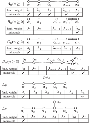
Figure 1. fundamental weight

It is known that $G_{2},F_{4}$ and $E_{8}$ have no minuscule weight. $G/P_{\lambda_{i}}$ can be described conveniently as a quotient of compact groups as follows.

$$(A_{n}\;\text{case})\;\; G/P_{i}\cong SU(n+1)/S(U(i)\times U(n+1-i))\cong Gr(k,n+1)$$

$$(B_{n}\;\text{case})\;\; G/P_{n}\cong SO(2n+1)/U(n)\cong OG(n,2n+1)$$

$$(C_{n}\;\text{case})\;\; G/P_{1}\cong Sp(n)/U(1)\times Sp(n-1)\cong\mathbb{C}P^{2n-1}$$

$$(D_{n}\;\text{case})\;\; G/P_{1}\cong SO(2n)/U(1)\times SO(2n-2)\cong Q_{2n-2},$$

$$G/P_{n-1}\cong SO(2n)/U(n)\cong S_{+},G/P_{n}\cong SO(2n)/U(n)\cong S_{-}$$

$$(E_{6}\;\text{case})\;\; G/P_{1}\cong G/P_{6}\cong E_{6}/SO(10)\times U(1)\cong\mathbb{O}P^{2}$$

$$(E_{7}\;\text{case})\;\; G/P_{1}\cong E_{7}/E_{6}\times U(1)$$

Here $OG(k,n)$ is the set of $k$-dimensional isotropic subspaces of $n$-dimensional complex vector space $V$ with a nondegenerate quadratic form. This is called the orthogonal Grassmannian. For $D_{n}$, $OG(n,2n)$ has two components $S_{+}$ and $S_{-}$. These are called varieties of pure spinors (or spinor varieties) and these are isomorphic to each other [Ma]. For $A_{n},B_{n},C_{n}$ and $D_{n}$, the minuscule representations are familiar (see section 6.5 in [BD]). For $A_{n}$, $V_{\lambda_{i}}$ is the exterior power $\bigwedge^{i}V_{\lambda_{1}}$ ($1\leq i\leq n$) where $V_{\lambda_{1}}$ is the standard representation on $\mathbb{C}^{n+1}$. For $B_{n}$, $V_{n}$ is the half-spin representation. For $C_{n}$, $V_{\lambda_{1}}$ is the standard representation on $\mathbb{C}^{2n}$. For $D_{n}$, $V_{\lambda_{1}}$ is the standard representation on $\mathbb{C}^{2n}$. $V_{\lambda_{n-1}}$ and $V_{\lambda_{n}}$ are the half-spin representations. We denote these two representations by $\Delta_{+}$ and $\Delta_{-}$. For exceptional groups, the minuscule representations are given in the section 5 of [Gec]. For $E_{6}$, $V_{\lambda_{1}}$ and $V_{\lambda_{6}}$ are $27$ dimensional representations. For $E_{7}$, $V_{\lambda_{1}}$ is a $56$ dimensional representation.

2.4. Minuscule weight orbits and simple roots

In this subsection, we observe relationships between minuscule weight orbits and the simple roots. Let $\lambda_{i}$ be a minuscule weight.

Proposition 11.

The set of all weights of $V_{\lambda_{i}}$ is the $W$-orbit of $\lambda_{i}$ and the multiplicities of all weights of $V_{\lambda_{i}}$ are one.

Proof.

It is obvious that $\sharp W/W_{P_{i}}\leq\text{dim}(W\cdot v_{\lambda_{i}})\leq\text{dim}(V_{\lambda_{i}})$. If there is a weight which has multiplicity more than one, then $\sharp W/W_{P_{i}}<\text{dim}V_{\lambda_{i}}$. Therefore by contraposition when we show that $\sharp W/W_{P_{i}}$ coincides with $\text{dim}_{\mathbb{C}}V_{\lambda_{i}}$, we obtain the statement of proposition 11.
We justify the above claim in each case. We have the orders of all Weyl groups from the table 2 in section 2.11 of [Hum]. For type $A_{n}$, we have $\text{dim}_{\mathbb{C}}\bigwedge{}^{i}\mathbb{C}^{n+1}=\binom{n+1}{i}$ ($1\leq i\leq n$). On the other hand, for this representation we have $W/W_{P_{i}}=\mathfrak{S}_{n+1}/(\mathfrak{S}_{i}\times\mathfrak{S}_{n+1-i})$. Therefore we obtain $\sharp W/W_{P_{i}}=\frac{(n+1)!}{i!(n+1-i)!}=\binom{n+1}{i}$. For type $B_{n}$, a minuscule representation is the half-spin representation and its dimension is $2^{n}$. Then $W/W_{P_{n}}=\mathfrak{S}_{n}\cdot(\mathbb{Z}_{2})^{n}/\mathfrak{S}_{n}$. Hence $\sharp W/W_{P_{n}}=2^{n}\cdot n!/n!=2^{n}$. For type $C_{n}$, a minuscule representation is the standard representation $\mathbb{C}^{2n}$ and its dimension is $2n$. The corresponding $W/W_{P_{1}}=\mathfrak{S}_{n}\cdot(\mathbb{Z}_{2})^{n}/\mathfrak{S}_{n-1}\cdot(\mathbb{Z}_{2})^{n-1}$. Hence $\sharp W/W_{P_{1}}=2^{n}\cdot n!/2^{n-1}\cdot(n-1)!=2n$. For type $D_{n}$, there are three minuscule representations. These are the standard representations and the two half-spin representations. These dimensions are $2n$, $2^{n-1}$, $2^{n-1}$ respectively. The corresponding $W/W_{P_{i}}$ ($i=1,n-1,n$) are $\mathfrak{S}_{n}\cdot(\mathbb{Z}_{2})^{n-1}/\mathfrak{S}_{n-1}\cdot(\mathbb{Z}_{2})^{n-2}$, $\mathfrak{S}_{n}\cdot(\mathbb{Z}_{2})^{n-1}/\mathfrak{S}_{n}$, $\mathfrak{S}_{n}\cdot(\mathbb{Z}_{2})^{n-1}/\mathfrak{S}_{n}$, and $\sharp W/W_{P_{i}}$($i=1,n-1,n$) are $2n$, $2^{n-1}$, $2^{n-1}$ respectively. For type $E_{6}$, there are two minuscule representations. These representations are both $27$ dimensional representations. The corresponding $W/W_{P_{1}}$ and $W/W_{P_{6}}$ are both $W_{E_{6}}/\mathfrak{S}_{5}\cdot(\mathbb{Z}_{2})^{4}$ where $W_{E_{6}}$ is the Weyl group of $E_{6}$. Then $\sharp W_{E_{6}}/\mathfrak{S}_{5}\cdot(\mathbb{Z}_{2})^{4}=2^{7}\cdot 3^{4}\cdot 5/2^{4}\cdot 5!=27$. For type $E_{7}$, the minuscule representation is a $56$ dimensional representation. The corresponding $W/W_{P_{1}}$ is $W_{E_{7}}/W_{E_{6}}$ where $W_{E_{7}}$ is the Weyl group of $E_{7}$. Then $\sharp W/W_{P_{1}}=2^{10}\cdot 3^{4}\cdot 5\cdot 7/2^{7}\cdot 3^{4}\cdot 5=56$. This completes the proof. ∎

From proposition 11, we have the weights of $V_{\lambda_{i}}$ as $\{v_{u(\lambda_{i})}|\;u\in{W^{P_{i}}}\}$ and the multiplication of these weights are all one. In addition, we know that the Weyl group is generated by the simple reflections $\{s_{\alpha_{j}}|\;j\in{\{1,\cdots,l\}}\}$. Therefore all weights can be obtained from $\lambda_{i}$ by applying $\{s_{\alpha_{j}}|\;j\in{\{1,\cdots,l\}}\}$ to $\lambda_{i}$ repeatedly. We use a canonical basis of $V_{\lambda_{i}}$ from section $5A.1$ of the article [Ja] with the following properties:

(2.1) $$e_{-\alpha_{j}}(v_{u(\lambda_{i})})=\begin{cases}v_{u(\lambda_{i})-\alpha_{j}}&(u(\lambda_{i}),\alpha_{j}^{\vee})=1\\ 0&\text{otherwise}.\end{cases}$$

(2.2) $$e_{\alpha_{j}}(v_{u(\lambda_{i})})=\begin{cases}v_{u(\lambda_{i})+\alpha_{j}}&(u(\lambda_{i}),\alpha_{j}^{\vee})=-1\\ 0&\text{\rm otherwise}.\end{cases}$$

$$H_{\alpha_{j}}(v_{u(\lambda_{i})})=(u(\lambda_{i}),\alpha_{j}^{\vee})v_{u(\lambda_{i})},$$

for all weights $u(\lambda_{i})$ and all $j\in{\{1,\cdots,l\}}$. As a consequence of (2.2), we have

(2.3) $$e_{\psi}(v_{u(\lambda_{i})})=\begin{cases}v_{u(\lambda_{i})+\psi}&(u(\lambda_{i}),\psi^{\vee})=-1\\ 0&\text{otherwise}.\end{cases}$$

2.5. Results

For any minuscule weight $\lambda_{i}$, the discussion in 2.3 establishes an isomorphism

$$V_{\lambda_{i}}=\bigoplus_{u(\lambda_{i})\in{W^{P}}\cdot\lambda_{i}}V_{u(\lambda_{i})}\cong H^{*}(G/P_{i};\mathbb{C}).$$

We remark that from section 2.3 this isomorphism is given by

$$V_{u(\lambda_{i})}\ni v_{u(\lambda_{i})}\leftrightarrow\sigma_{u}\in{H^{2\ell(u)}(G/P_{i});\mathbb{C}}$$

for all $u\in{W^{P_{i}}}$. From this it can be seen that the cohomology grading on the right corresponds to the grading by simple roots on the left.
Now we can state our main theorem.

Theorem 12.

Fix $\mathfrak{g}$ and a minuscule weight $\lambda_{i}$. There is a natural correspondence between (i) the asymptotic data

$$m=-h_{0}=-\sum_{j=1}^{l}r_{j}H_{\alpha_{j}}\in{\mathfrak{h}_{\sharp}}$$

and (ii) the DPW data

$$\omega=\frac{1}{\lambda}\left(\sum_{j=1}^{l}e_{-\alpha_{j}}+qe_{\psi}\right)\frac{dq}{q}$$

for solutions of the tt*-Toda equations. The asymptotic data corresponds to a unique global solution when $\mathfrak{g}$ has type $A_{n}$ (and conjecturally for any $\mathfrak{g}$). The holomorphic data correspond to the Dubrovin connection for the quantum cohomology of $G/P_{i}$, i.e. the natural action of $\sum_{j=1}^{l}e_{-\alpha_{j}}+qe_{\psi}$ corresponds to quantum multiplication by a generator of $H^{2}(G/P_{i},\mathbb{C})$.

Proof.

In the bijection of Theorem 4 (section 2.1), we see that $m=-h_{0}$ corresponds to the origin of the fundamental Weyl alcove, and in this case we have $k_{0}=0$ and $k_{1}=\cdots=k_{l}=-1$. This gives the correspondence between (i) and (ii) (with $q=z$). For the statement concerning global solutions, we refer to [GIL], [Mo]. The identification of $\omega$ with the Dubrovin connection can be extracted from [GM], but we shall present a new and more direct proof in the next section. ∎

Remark 13.

(On the Satake isomorphism) When $\mathfrak{g}$ is of type $A_{n}$ (or, conjecturally, of type $D_{n}$,$E_{6}$), the same global solution corresponds to the Dubrovin connection of any minuscule weight. This suggests a relation between the quantum cohomology algebra of the corresponding flag manifolds. In the $A_{n}$ case this can be stated as

$$\textstyle\bigwedge^{k}QH^{*}(\mathbb{C}P^{n})\cong QH^{*}Gr(k,n+1)$$

(see [GM] for further explanation).
In the $D_{n}$ case, the analogous relation is:

(2.4) $$\textstyle\bigwedge_{\pm}^{half}QH^{*}(Q_{2n-2})\cong\text{End}_{\mathbb{C}}(QH^{*}(S_{\pm})).$$

This follows from theorem 12 when we identify $H^{*}(Q_{2n-2};\mathbb{C})$ with $\mathbb{C}^{2n}$ and $H^{*}(S_{\pm};\mathbb{C})$ with $\Delta_{\pm}$, because (2.4) corresponds to the well known relation

$$\textstyle\bigwedge_{\pm}^{half}\mathbb{C}^{2n}\cong\text{End}_{\mathbb{C}}(\Delta_{\pm}).$$

In order to explain the notation, we recall the relation here. We denote a positively oriented orthonormal basis of $\mathbb{C}^{2n}$ by $e_{1},\cdots,e_{2n}$. We define the isomorphism $\star:\textstyle\bigwedge^{i}\mathbb{C}^{2n}\rightarrow\textstyle\bigwedge^{2n-i}\mathbb{C}^{2n}$ by

$$\star(e_{\xi(1)}\wedge e_{\xi(2)}\wedge\cdots\wedge e_{\xi(i)})=\text{sign}(\xi)e_{\xi(i+1)}\wedge e_{\xi(i+2)}\wedge\cdots\wedge e_{\xi(2n)}$$

for any permutation $\xi$. Then we obtain $\star\cdot\star=(-1)^{i(2n-i)}\text{id}$. We define $\iota:=(-i)^{n}\star:\bigwedge^{n}\mathbb{C}^{2n}\rightarrow\bigwedge^{n}\mathbb{C}^{2n}$. Then $\iota\cdot\iota=\text{id}$. Thus we have the canonical eigenspace decomposition $\bigwedge^{n}\mathbb{C}^{2n}\cong\bigwedge_{+}^{n}\mathbb{C}^{2n}\oplus\bigwedge_{-}^{n}\mathbb{C}^{2n}$. If $n=2m+1$, then we define $\bigwedge_{\pm}^{half}\mathbb{C}^{2n}$ by

$$\textstyle\bigwedge^{0}\mathbb{C}^{4m+2}\bigoplus\textstyle\bigwedge^{2}\mathbb{C}^{4m+2}\bigoplus\cdots\bigoplus\textstyle\bigwedge^{2m}\mathbb{C}^{4m+2}.$$

If $n=2m$, then we define $\bigwedge_{+}^{half}\mathbb{C}^{2n}$ by

$$\textstyle\bigwedge^{0}\mathbb{C}^{4m}\bigoplus\textstyle\bigwedge^{2}\mathbb{C}^{4m}\bigoplus\cdots\bigoplus\textstyle\bigwedge_{+}^{2m}\mathbb{C}^{4m}.$$

and $\bigwedge_{-}^{half}\mathbb{C}^{2n}$ by

$$\textstyle\bigwedge^{0}\mathbb{C}^{4m}\bigoplus\textstyle\bigwedge^{2}\mathbb{C}^{4m}\bigoplus\cdots\bigoplus\textstyle\bigwedge_{-}^{2m}\mathbb{C}^{4m}.$$

From Theorem (6.2) of [BD], we have

$$\Delta_{+}\otimes\Delta_{+}=\textstyle\bigwedge_{+}^{n}+\textstyle\bigwedge^{n-2}+\cdots$$

$$\Delta_{+}\otimes\Delta_{-}=\textstyle\bigwedge^{n-1}+\textstyle\bigwedge^{n-3}+\cdots$$

$$\Delta_{-}\otimes\Delta_{-}=\textstyle\bigwedge_{-}^{n}+\textstyle\bigwedge^{n-2}+\cdots$$

as $\mathfrak{spin}(2n)$ representations where the last terms are $\bigwedge^{4}+\bigwedge^{2}+\bigwedge^{0}$ or $\bigwedge^{3}+\bigwedge^{1}$. If $n=2m+1$, then we have

$$\text{End}_{\mathbb{C}}(\Delta_{+}) \cong\Delta_{+}^{*}\otimes\Delta_{+}\cong\Delta_{+}\otimes\Delta_{-}$$

$$\cong\textstyle\bigwedge^{2m}+\textstyle\bigwedge^{2m-2}+\cdots+\textstyle\bigwedge^{2}+\textstyle\bigwedge^{0}$$

$$=\textstyle\bigwedge_{\pm}^{half}\mathbb{C}^{4m+2}.$$

If $n=2m$, then we have

$$\text{End}_{\mathbb{C}}(\Delta_{+}) \cong\Delta_{+}^{*}\otimes\Delta_{+}\cong\Delta_{+}\otimes\Delta_{+}$$

$$\cong\textstyle\bigwedge_{+}^{2m}+\bigwedge^{2m-2}+\cdots+\bigwedge^{2}+\bigwedge^{0}$$

$$=\textstyle\bigwedge_{+}^{half}\mathbb{C}^{4m}.$$

When we consider the minuscule $\Delta_{-}$ and the corresponding homogeneous space $S_{-}$, we obtain

$$\textstyle\bigwedge_{-}^{half}QH^{*}(Q_{2n-2})\cong\text{End}_{\mathbb{C}}(QH^{*}(S_{-}))$$

as in the case of $\Delta_{+}$.

3. Completion of the proof of the main theorem

We consider the irreducible representations $V_{\lambda_{i}}$ whose highest weight are minuscule weights $\lambda_{i}$ (see table in section 2.3). In this section we use results on quantum cohomology to prove that the quantum multiplication by the generator of the second cohomology coincides with the endomorphism $\sum_{j=1}^{l}e_{-\alpha_{j}}+qe_{\alpha_{\psi}}$ for a minuscule representation $V_{\lambda_{i}}$. To show this statement, we use the quantum Chevalley formula.

Theorem 14.

([FW]) For $\beta\in{\Pi\backslash\Pi_{P_{i}}}$ and $u\in{W^{P_{i}}}$, we have the quantum product $\circ$ by $\sigma_{\beta}$ as

$$\sigma_{s_{\beta}}\circ\sigma_{u}= \sum_{\ell(us_{\alpha})=\ell(u)+1}(\lambda_{\beta},\alpha^{\vee})\sigma_{us_{\alpha}}$$

$$+\sum_{l(us_{\alpha})=l(u)-n_{\alpha}+1}(\lambda_{\beta},\alpha^{\vee})\sigma_{us_{\alpha}}\cdot q^{d(\alpha)}$$

where $\alpha$ ranges over $\triangle^{+}\backslash\triangle_{P_{i}}^{+}$, $\lambda_{\beta}$ is the fundamental weight corresponding to $\beta$,

$$n_{\alpha}=(\sum_{\gamma\in{\triangle^{+}\backslash\triangle_{P_{i}}^{+}}}\gamma,\alpha^{\vee})$$

and

$$d(\alpha)=\sum_{\beta\in{\Pi\backslash\Pi_{P_{i}}}}(\lambda_{\beta},\alpha^{\vee})\sigma(s_{\beta}),$$

and where $\sigma(s_{\beta})$ is the homology class of $H_{2}(G/P_{i})$ which is Poincaré dual to $\sigma_{s_{\beta}}$.

In our situation, $\Pi\backslash\Pi_{P_{i}}=\{\alpha_{i}\}$. Therefore the generator of the second cohomology is only $\sigma_{s_{\alpha_{i}}}$ and $\lambda_{\beta}=\lambda_{i}$. We have $d(\alpha)=(\lambda_{i},\alpha^{\vee})\sigma(s_{\alpha_{i}})=\sigma(s_{\alpha_{i}})$ for $\alpha\in{\triangle^{+}\backslash\triangle^{+}_{P_{i}}}$ because $\lambda_{i}$ is a minuscule weight. We consider $q^{\sigma(s_{\beta})}$ only as a complex parameter $q$ in $\mathbb{C}$.
From lemma 3.5 in [FW], the first Chern class of $G/P_{i}$ is $n_{\alpha}$ times a generator of $H^{2}(G/P_{i})$, and by [CMP], we know that $n_{\alpha}$ is the Coxeter number $s$. Explicitly, we have $n_{\alpha}=n+1$ ($A_{n}$ type), $n_{\alpha}=2n$ ($B_{n}$ type), $n_{\alpha}=2n$ ($C_{n}$ type), $n_{\alpha}=2n-2$ ($D_{n}$ type), $n_{\alpha}=12$ ($E_{6}$ type), $n_{\alpha}=18$ ($E_{7}$ type) for all $\alpha\in{\triangle^{+}\backslash\triangle_{P_{i}}^{+}}$.
Then we have the quantum Chevalley formula as follows.

$$\sigma_{s_{\alpha_{i}}}\circ\sigma_{u}= \sum_{\ell(us_{\alpha})=\ell(u)+1}(\lambda_{i},\alpha^{\vee})\sigma_{us_{\alpha}}$$

$$+\sum_{\ell(us_{\alpha})=\ell(u)-(s-1)}(\lambda_{i},\alpha^{\vee})\sigma_{us_{\alpha}}\cdot q$$

where $\alpha\in{\triangle^{+}\backslash\triangle_{P_{i}}^{+}}$.
To replace the conditions of these summations, the following lemma, corollary and proposition are key ingredients.

Lemma 15.

Let $\lambda_{i}$ be a minuscule weight. For $u\in{W^{P_{i}}}$ and $\alpha\in{\Pi}$, we have the three following situations.
(I) $(u(\lambda_{i}),\alpha^{\vee})=1\Leftrightarrow\ell(s_{\alpha}u)=\ell(u)+1$.
(II) $(u(\lambda_{i}),\alpha^{\vee})=0\Leftrightarrow\ell(s_{\alpha}u)=\ell(u)$.
(III) $(u(\lambda_{i}),\alpha^{\vee})=-1\Leftrightarrow\ell(s_{\alpha}u)=\ell(u)-1$.
Here we consider the length function $l(u)$ in $W^{P_{i}}$.

Proof.

(a) First we show the implication ($\Rightarrow$), for each of (I), (II), (III). Here we do not use the minuscule condition.
(I) We assume $(u(\lambda_{i}),\alpha^{\vee})=1$. We show $s_{\alpha}u\in{W^{P_{i}}}$. If $(u(\lambda_{i}),\alpha^{\vee})=1$, $(\lambda_{i},u^{-1}(\alpha)^{\vee})=1$ and $u^{-1}(\alpha)$ is a positive root. Therefore $\ell(s_{\alpha}u)=\ell(u)+1$ in $W$ (see section 1.6 in [Hum]). For $\beta\in{\Pi_{P_{i}}}$, we have

$$(\lambda_{i},(us_{\beta})^{-1}(\alpha)^{\vee})>0 \Leftrightarrow(\lambda_{i},s_{\beta}u^{-1}(\alpha)^{\vee})>0$$

$$\Leftrightarrow(s_{\beta}(\lambda_{i}),u^{-1}(\alpha)^{\vee})>0$$

$$\Leftrightarrow(\lambda_{i},u^{-1}(\alpha)^{\vee})>0$$

Therefore we have $(\lambda_{i},(us_{\beta})^{-1}(\alpha)^{\vee})>0$. Hence $\ell(s_{\alpha}us_{\beta})>\ell(us_{\beta})$. On the other hand, for all $\beta\in{\Pi_{P_{i}}}$, we have $\ell(us_{\beta})>\ell(u)$ because $u$ is in $W^{P_{i}}$. Hence $\ell(us_{\beta})=\ell(u)+1$ in $W$. Thus we have

$$\ell(s_{\alpha}u)=\ell(us_{\beta})<\ell(s_{\alpha}us_{\beta}).$$

This means that $s_{\alpha}u\in{W^{P_{i}}}$. Therefore we obtain $\ell(s_{\alpha}u)=\ell(u)+1$ in $W^{P_{i}}$.
(II) We assume $(u(\lambda_{i}),\alpha^{\vee})=0$. We show $s_{u^{-1}(\alpha)}\in{W_{P_{i}}}$. Let $u^{-1}(\alpha)^{\vee}=b_{1}\alpha_{1}^{\vee}+\cdots+b_{l}\alpha_{l}^{\vee}$ ($b_{i}\in{\mathbb{R}}$). Then we have

$$(\lambda_{i},u^{-1}(\alpha)^{\vee})=b_{i}=0$$

Therefore $u^{-1}(\alpha)\in{\triangle_{P_{i}}}$ and $s_{u^{-1}(\alpha)}\in{W_{P_{i}}}$. We obtain

$$\ell(s_{\alpha}u)=\ell(us_{u^{-1}(\alpha)})=\ell(u)\;\text{in}\;W^{P_{i}}.$$

(III) We assume $(u(\lambda_{i}),\alpha^{\vee})=-1$. We show $s_{\alpha}u\in{W^{P_{i}}}$. If $(u(\lambda_{i}),\alpha^{\vee})=-1$, then $(\lambda_{i},u^{-1}(\alpha)^{\vee})=-1<0$. $u^{-1}(\alpha)$ is a negative root. Hence we have

$$\ell(s_{\alpha}u)=\ell(u)-1<\ell(u)<\ell(us_{\beta})\;\text{in}\;W$$

for $\beta\in{\Pi_{P_{i}}}$. Now we have

$$\ell(us_{\beta})=\ell(u)+1=\ell(s_{\alpha}u)+2\;\text{in}\;W.$$

Let $\ell(us_{\beta})=r$. Then $\ell(s_{\alpha}us_{\beta})=r-1,r+1$ and $\ell(s_{\alpha}u)=r-2$. So $\ell(s_{\alpha}us_{\beta})>\ell(s_{\alpha}u)$. This means that $s_{\alpha}u\in{W^{P_{i}}}$. Thus we obtain $\ell(s_{\alpha}u)=\ell(u)-1$ in $W^{P_{i}}$.
(b) Next we show the implication ($\Leftarrow$), for each of (I), (II), (III). For (I), we assume $\ell(s_{\alpha u})=\ell(u)+1$. Since $\lambda_{i}$ is minuscule, $(u(\lambda_{i}),\alpha^{\vee})$ takes only the values $1,0,-1$. If $(u(\lambda_{i}),\alpha^{\vee})$ is $0$ or $-1$, we obtain a contradiction, by part (a). The proofs in the case (II), (III) are similar. ∎

Now we have the weights of $V_{\lambda_{i}}$ as $\lambda_{i}-\sum_{j=1}^{l}n_{j}\alpha_{j}$ where $n_{j}\in{\mathbb{Z}_{\geq 0}}$. From this lemma, we obtain the following corollary.

Corollary 16.

For $u\in{W^{P_{i}}}$ such that $u(\lambda_{i})=\lambda_{i}-\sum_{j=1}^{l}n_{j}\alpha_{j}$, we have $\ell(u)=\sum_{j=1}^{l}n_{j}$.

Proof.

We have

$$\ell(s_{\alpha_{j}}u)=\ell(u)+1 \Leftrightarrow(u(\lambda_{i}),\alpha_{j}^{\vee})=1$$

$$\Leftrightarrow s_{\alpha_{j}}(u(\lambda_{i}))=u(\lambda_{i})-\alpha_{j}$$

by lemma 15. The elements of $W^{P_{i}}$ are described by a product of simple reflections. Thus $\ell(u)=\sum_{j=1}^{l}n_{j}$. ∎

We have the following proposition.

Proposition 17.

(I) If there exist $\alpha\in{\triangle^{+}}$ such that $\ell(s_{\alpha}u)=\ell(u)+1$ for $u\in{W^{P_{i}}}$, then $\alpha\in{\Pi}$ and $(u(\lambda_{i}),\alpha^{\vee})=1$.
(II) If there exist $\alpha\in{\triangle^{+}}$ such that $\ell(s_{\alpha}u)=\ell(u)-(s-1)$ for $u\in{W^{P_{i}}}$, then $\alpha=\psi$ and $(u(\lambda_{i}),\psi^{\vee})=-1$.

Proof.

(I) For $\alpha\in{\triangle^{+}}$ such that $\ell(s_{\alpha}u)=\ell(u)+1$, we have

$$s_{\alpha}u(\lambda_{i})=u(\lambda_{i})-(u(\lambda_{i}),\alpha^{\vee})\alpha.$$

By the assumption that $\ell(s_{\alpha}u)>\ell(u)$, we have $(u(\lambda_{i}),\alpha^{\vee})=1$ and $\alpha$ must be a simple root by corollary 16.
(II) For $\alpha\in{\triangle^{+}}$ such that $\ell(s_{\alpha}u)=\ell(u)-(s-1)$. Then we have

$$s_{\alpha}u(\lambda_{i})=u(\lambda_{i})-(u(\lambda_{i}),\alpha^{\vee})\alpha.$$

By the assumption $\ell(s_{\alpha}u)<\ell(u)$, we have $(u(\lambda_{i}),\alpha^{\vee})=-1$. When $\alpha=\sum_{j=1}^{l}q_{j}\alpha_{j}$, then $\alpha$ must be $\psi$ because there is only one positive root which has the height $\sum_{j=1}^{l}q_{j}=s-1$. ∎

By using the relation $us_{\alpha}=s_{u(\alpha)}u=s_{-u(\alpha)}u$, corollary 16 and proposition 17, we can replace the conditions of the summation in the quantum Chevalley formula.
We show that we can simplify the first summation to

$$\sum_{(u(\lambda_{i}),\alpha^{\prime\vee})=1,\alpha^{\prime}\in{\Pi}}\sigma_{s_{\alpha^{\prime}}u}$$

by setting $\alpha^{\prime}=u(\alpha)$. Then we shall show that $\alpha^{\prime}$ is a positive root. In fact, if $\alpha^{\prime}$ is a negative root, then $(u(\lambda_{i}),\alpha^{\prime\vee})=-1$ satisfies $\ell(s_{\alpha^{\prime}}u)=\ell(u)+1$. However this contradicts $\alpha\in{\triangle^{+}\backslash\triangle_{P_{i}}^{+}}$ because we have

$$(u(\lambda_{i}),\alpha^{\prime\vee})=-1\Leftrightarrow(u(\lambda_{i}),u(\alpha^{\vee}))=-1\Leftrightarrow(\lambda_{i},\alpha^{\vee})=-1.$$

Thus $\alpha^{\prime}$ is in $\triangle^{+}$. By proposition 17, we have $\alpha^{\prime}\in{\Pi}\subset{\triangle^{+}}$. Hence we have

$$\sum_{\ell(us_{\alpha})=\ell(u)+1}(\lambda_{i},\alpha^{\vee})\sigma_{us_{\alpha}}=\sum_{(u(\lambda_{i}),\alpha^{\prime\vee})=1,\alpha^{\prime}\in{\Pi}}\sigma_{s_{\alpha^{\prime}}u}$$

as the first summation of $\sigma_{s_{\alpha_{i}}}\circ\sigma_{u}$.
For the second summation, let $\alpha^{\prime}=-u(\alpha)$. Then we shall show that $\alpha^{\prime}$ is also a positive root. In fact, if $\alpha^{\prime}$ is a negative root, then $(u(\lambda_{i}),\alpha^{\prime\vee})=1$ satisfies $\ell(s_{\alpha^{\prime}}u)=\ell(u)-(s-1)$. However this contradicts $\alpha\in{\triangle^{+}\backslash\triangle_{P_{i}}^{+}}$ because we have

$$(u(\lambda_{i}),\alpha^{\prime\vee})=1\Leftrightarrow(u(\lambda_{i}),-u(\alpha^{\vee}))=1\Leftrightarrow(\lambda_{i},\alpha^{\vee})=-1.$$

Thus $\alpha^{\prime}=-u(\alpha)$ is in $\triangle^{+}$ for $\alpha\in{\triangle^{+}\backslash\triangle_{P_{i}}^{+}}$. By proposition 17, we have $\alpha^{\prime}=\psi$ and $(u(\lambda_{i}),\psi^{\vee})=-1$. Hence for the second summation of $\sigma_{s_{\alpha_{i}}}\circ\sigma_{u}$ we have

$$\sum_{\ell(us_{\alpha})=\ell(u)-(s-1)}(\lambda_{i},\alpha^{\vee})\sigma_{us_{\alpha}}\cdot q$$

$$= \sum_{\ell(s_{\alpha^{\prime}}u)=\ell(u)-(s-1)}(\lambda_{i},-u^{-1}(\alpha^{\prime\vee}))\sigma_{s_{\alpha^{\prime}}u}\cdot q$$

$$= \begin{cases}q\sigma_{s_{\psi}u}&(u(\lambda_{i}),\psi^{\vee})=-1\\ 0&\text{\rm otherwise}.\end{cases}$$

Thus we obtain

$$\sigma_{s_{\alpha_{i}}}\circ\sigma_{u}=\begin{cases}\displaystyle\sum_{(u(\lambda_{i}),\alpha_{j}^{\vee})=1}\sigma_{s_{\alpha_{j}}u}+q\sigma_{s_{\psi}u}&(u(\lambda_{i}),\psi^{\vee})=-1\\ \displaystyle\sum_{(u(\lambda_{i}),\alpha_{j}^{\vee})=1}\sigma_{s_{\alpha_{j}}u}&\text{\rm otherwise}.\end{cases}$$

On the other hand, for $v_{u(\lambda_{i})}$ we have

$$(\sum_{j=1}^{l}e_{-\alpha_{j}}+qe_{\psi})\cdot v_{u(\lambda_{i})}$$

$$= \begin{cases}\displaystyle\sum_{(u(\lambda_{i}),\alpha_{j}^{\vee})=1}v_{u(\lambda_{i})-\alpha_{j}}+qv_{u(\lambda_{i})+\psi}&(u(\lambda_{i}),\psi^{\vee})=-1\\ \displaystyle\sum_{(u(\lambda_{i}),\alpha_{j}^{\vee})=1}v_{u(\lambda_{i})-\alpha_{j}}&\text{\rm otherwise}\end{cases}$$

$$= \begin{cases}\displaystyle\sum_{(u(\lambda_{i}),\alpha_{j}^{\vee})=1}v_{s_{\alpha_{j}}u(\lambda_{i})}+qv_{s_{\psi}u(\lambda_{i})}&(u(\lambda_{i}),\psi^{\vee})=-1\\ \displaystyle\sum_{(u(\lambda_{i}),\alpha_{j}^{\vee})=1}v_{s_{\alpha_{j}}u(\lambda_{i})}&\text{\rm otherwise}\end{cases}$$

by using the definitions of (2.1) and (2.3). Therefore we obtain

$$\sum_{j=1}^{l}e_{-\alpha_{j}}+qe_{\psi}=\sigma_{s_{\alpha_{i}}}\circ.$$

Department of Mathematics
Faculty of Science and Engineering
Waseda University
3-4-1 Okubo, Shinjuku, Tokyo 169-8555
JAPAN

References

• [BD] T. Bröcker and T. tom Dieck, Representations of Compact Lie Groups, Springer, 1985.
• [CV] S. Cecotti and C. Vafa, Topological—anti-topological fusion, Nuclear Phys. B 367 (1991), 359-461.
• [CMP] P. E. Chaput, L. Manivel, and N. Perrin, Quantum cohomology of minuscule homogeneous spaces. II. Hidden symmetries, Int. Math. Res. Not. IMRN 2007, 1-29.
• [DGR] J. F. Dorfmeister, M. A. Guest, and W. Rossman, The tt* structure of the quantum cohomology of $\mathbb{C}P^{1}$ from the viewpoint of differential geometry, Asian J. Math. 14 (2010), 417-438.
• [Dub] B. Dubrovin, Geometry and integrability of topological-antitopological fusion, Comm. Math. Phys. 152 (1993), 539-564.
• [FW] W. Fulton and C. Woodward, On the quantum product of Schubert classes, J. Algebraic Geom., 13 (2004), 641–661.
• [Gec] M. Geck, Minuscule weights and Chevalley groups, Finite Simple Groups: Thirty Years of the Atlas and Beyond, Contemporary Math., Amer. Math. Soc., 694 (2017), 159-176.
• [GM] V. Golyshev and L. Manivel, Quantum cohomology and the Satake isomorphism, arxiv:1106.3120.
• [G1] M. A. Guest, Harmonic Maps, Loop Groups and Integrable Systems, LMS Student Texts 38, Cambridge Univ. Press, 1997.
• [G2] M. A. Guest, From Quantum Cohomology to Integrable Systems, Oxford Univ. Press, 2008.
• [GH] M. A. Guest and N.-K. Ho, Kostant, Steinberg, and the Stokes matrices of the tt*-Toda equations, Selecta Math. (N.S.), 25 (2019), no. 50.
• [GIL] M. A. Guest, A. Its and C. S. Lin, Isomonodromy aspects of the tt* equations of Cecotti and Vafa III. Iwasawa factorization and asymptotics, Commun. Math. Phys. 374 (2020), 923-973.
• [GL1] M. A. Guest and C.-S. Lin, Some tt* structures and their integral Stokes data, Comm. Number Theory Phys. 6 (2012), 785–803.
• [GL2] M. A. Guest and C.-S. Lin, Nonlinear PDE aspects of the tt* equations of Cecotti and Vafa, J. reine angew. Math. 689 (2014), 1-32.
• [Hil] H. Hiller, Geometry of Coxeter Groups, Research Notes in Mathematics, No.54, Pitman, Boston, 1982.
• [Hit] N. J. Hitchin, Lie groups and Teichmüller space, Topology 31 (1992), 449-473.
• [Hum] J. Humphreys, Reflection Groups and Coxeter Groups, Cambridge University Press, Cambridge, 1990.
• [Ir] H. Iritani, Real and integral structures in quantum cohomology I: toric orbifolds, arXiv:0712.2204.
• [Ja] J. C. Jantzen, Lectures on Quantum Groups, Graduate Studies in Mathematics, vol. 6, American Mathematical Society, Providence, RI, 1996.
• [Ko] B. Kostant, The principal three-dimensional subgroup and the Betti numbers of a complex simple Lie group, Am. J. Math. 81 (1959), 973-1032.
• [LT] T. Lam and N. Templier, The mirror conjecture for minuscule flag varieties, arXiv:1705.00758.
• [Ma] L. Manivel, Double spinor Calabi-Yau varieties, arXiv:1709.07736v2.
• [Mo] T. Mochizuki, Harmonic bundles and Toda lattices with opposite sign, arXiv:1301.1718.
• [Yo] I. Yokota, Exceptional Lie groups, arXiv:0902.0431.