Robust and Efficient Multilevel-ILU Preconditioning of Hybrid
Newton-GMRES for Incompressible Navier-Stokes Equations

Abstract

[Summary]We introduce a robust and efficient preconditioner for a hybrid Newton-GMRES method for solving the nonlinear systems arising from incompressible Navier-Stokes equations. When the Reynolds number is relatively high, these systems often involve millions of degrees of freedom (DOFs), and the nonlinear systems are difficult to converge, partially due to the strong asymmetry of the system and the saddle-point structure. In this work, we propose to alleviate these issues by leveraging a multilevel ILU preconditioner called HILUCSI, which is particularly effective for saddle-point problems and can enable robust and rapid convergence of the inner iterations in Newton-GMRES. We further use Picard iterations with the Oseen systems to hot-start Newton-GMRES to achieve global convergence, also preconditioned using HILUCSI. To further improve efficiency and robustness, we use the Oseen operators as physics-based sparsifiers when building preconditioners for Newton iterations and introduce adaptive refactorization and iterative refinement in HILUCSI. We refer to the resulting preconditioned hybrid Newton-GMRES as HILUNG. We demonstrate the effectiveness of HILUNG by solving the standard 2D driven-cavity problem with Re 5000 and a 3D flow-over-cylinder problem with low viscosity. We compare HILUNG with some state-of-the-art customized preconditioners for INS, including two variants of augmented Lagrangian preconditioners and two physics-based preconditioners, as well as some general-purpose approximate-factorization techniques. Our comparison shows that HILUNG is much more robust for solving high-Re problems and it is also more efficient in both memory and runtime for moderate-Re problems.

1 Introduction

Incompressible Navier-Stokes (INS) equations are widely used for modeling fluids. The time-dependent INS equations (after normalizing density) read

$$\partial\boldsymbol{u}/\partial t-\nu\Delta\boldsymbol{u}+\boldsymbol{u}\cdot\boldsymbol{\nabla u}+\boldsymbol{\nabla}p =\boldsymbol{g},$$ (1)

$$\boldsymbol{\nabla}\cdot\boldsymbol{u} =0,$$ (2)

where $\boldsymbol{u}$ and $p$ are velocities and pressure, respectively, and $\nu$ is the kinetic viscosity. These equations can be solved using a semi-implicit or fully implicit scheme.¹ A fully implicit method can potentially enable larger time steps, but it often leads to large-scale nonlinear systems of equations, of which robust and efficient solution has been an active research topic in the past two decades.^{2, 3, 4, 5} A main challenge in a fully implicit method is to solve the stationary or quasi-steady INS equation, in which the momentum equation (1) becomes

$$-\nu\Delta\boldsymbol{u}+\boldsymbol{u}\cdot\boldsymbol{\nabla u}+\boldsymbol{\nabla}p=\boldsymbol{g},$$ (3)

which is mathematically equivalent to (1) as the time step approaches infinity. In this work, we focus on solving the stationary INS equations. A standard technique to solve this nonlinear system is to use some variants of truncated (aka inexact) Newton methods,⁶ p.284 which solve the linearized problem approximately at each step, for example, using an iterative method.⁷ Assume INS equations are discretized using finite elements, such as using the Taylor-Hood finite-element spaces.⁸ At each truncated Newton’s step, one needs to approximately solve a linear system

$$\begin{bmatrix}\boldsymbol{A}&\boldsymbol{E}^{T}\\ \boldsymbol{E}&\boldsymbol{0}\end{bmatrix}\begin{bmatrix}\delta\boldsymbol{u}_{k}\\ \delta p_{k}\end{bmatrix}\approx-\begin{bmatrix}\boldsymbol{f}_{k}\\ \boldsymbol{h}_{k}\end{bmatrix},$$ (4)

where $\delta\boldsymbol{u}_{k}$ and $\delta p_{k}$ correspond to the increments of $\boldsymbol{u}$ and $p$, respectively; see, e.g., Elman et al.² for a detailed derivation. Let

$$\boldsymbol{A}=\boldsymbol{K}+\boldsymbol{C}_{k}+\boldsymbol{W}_{k},$$

where $\boldsymbol{K}$, $\boldsymbol{C}_{k}$, and $\boldsymbol{W}_{k}$ correspond to $\nu\Delta\boldsymbol{u}$, $\boldsymbol{u}_{k}\cdot\boldsymbol{\nabla u}$, and $\boldsymbol{u}\cdot\boldsymbol{\nabla u}_{k}$, respectively. In a so-called hybrid nonlinear method,^{6, 9} inexact Newton methods may be “hot-started” using more robust but more slowly converging methods, such as some Picard iterations. In the context of INS, a particularly effective hot starter is the Picard iteration with the Oseen system,² which solve the simplified and sparser linear system

$$\begin{bmatrix}\boldsymbol{K}+\boldsymbol{C}_{k}&\boldsymbol{E}^{T}\\ \boldsymbol{E}&\boldsymbol{0}\end{bmatrix}\begin{bmatrix}\delta\boldsymbol{u}_{k}\\ \delta p_{k}\end{bmatrix}\approx-\begin{bmatrix}\boldsymbol{f}_{k}\\ \boldsymbol{h}_{k}\end{bmatrix}.$$ (5)

In the linear-algebra literature,¹⁰ Eqs. (4) and (5) are often referred to as (generalized) saddle-point problems, which are notoriously difficult to solve robustly and efficiently at a large scale. One of the bottlenecks in solving these nonlinear systems, both in terms of robustness and efficiency, is the iterative solver of the linear systems at each nonlinear step. The aim of this paper is to overcome this bottleneck by developing a robust and efficient preconditioner for those iterative linear solvers in the inner iterations of a truncated Newton method with hot start for solving the INS.

For large-scale systems of nonlinear equations, a successful class of truncated Newton methods is the Newton-Krylov methods¹¹ (including Jacobian-free Newton-Krylov methods^{12, 13}), which utilizes Krylov subspace methods (such as GMRES¹⁴) to approximate the linear solve. Implementations of such methods can be found in some general-purpose nonlinear solver libraries, such as NITSOL,¹⁵ MOOSE,¹⁶ and SNES¹⁷ in PETSc.¹⁸ However, the INS equations pose significant challenges when the Reynolds number (i.e., $\text{Re}\equiv\|\boldsymbol{u}\|L/\nu$ with respect to some reference length $L$) is high, due to steep boundary layers and potential corner singularities.^{1, 19} Although one may improve robustness using some generic techniques such as damping (aka backtracking),⁹ they often fail for INS.²⁰ In recent years, preconditioners have been recognized as critical techniques in improving the robustness and efficiency of nonlinear INS solvers. Some of the most successful preconditioners include (block) incomplete LU,^{21, 22} augmented Lagrangian methods,^{23, 24, 25, 26} and block preconditioners with approximate Schur complements.^{22, 27} They have been shown to be effective for INS equations with moderate Re (e.g., up to $2000$)^{22, 27}, regularized flows,²⁸ or compressible and Reynolds averaged Navier-Stokes (RANS) equations with a wide range of Re,²¹ but challenges remained for INS with higher Re (see Section 4.1). In addition, higher Re also requires finer meshes, which lead to larger-scale systems with millions and even billions of degrees of freedom (DOFs),²⁹ posing significant challenges in the scalability of the preconditioners with respect to the problem size.

To address these challenges, we propose a new type of preconditioner for Newton-GMRES for the INS, based on a multilevel incomplete LU (MLILU) technique. We build our preconditioner based on HILUCSI (or Hierarchical Incomplete LU-Crout with Scalability-oriented and Inverse-based dropping), which the authors and co-workers introduced recently for indefinite linear systems from partial differential equations (PDEs), such as saddle-point problems.³⁰ In this work, we incorporate HILUCSI into Newton-GMRES to develop HILUNG, for nonlinear saddle-point problems from Navier-Stokes equations. To this end, we introduce sparsifying operators based on (4) and (5), develop adaptive refactorization and thresholding to avoid potential “over-factorization” (i.e., too dense incomplete factorization or too frequent refactorization), and introduce iterative refinement during preconditioning to reduce memory requirement. As a result, HILUNG can robustly solve the standard (instead of the regularized) 2D driven-cavity problem with Re $5000$ without stabilization or regularization. In contrast, the state-of-the-art block preconditioner based on approximate Schur complements^{31, 32} and (modified) augmented Lagrangian methods^{23, 24, 25, 26} failed to converge at Re $1000$ and/or Re $5000$ with a similar configuration, respectively. In addition, we show that HILUNG also improved the efficiency over another general-purpose multilevel ILU preconditioner³³ by a factor of 34 for the 3D flow-over-cylinder problem with one million DOFs, and enabled an efficient solution of the problem with about ten million DOFs using only 60GB of RAM, while other alternatives ran out of memory. We have released the core component of HILUNG, namely HILUCSI, as an open-source library at https://github.com/hifirworks/hifir.

The remainder of the paper is organized as follows. Section 2 reviews some background on truncated and inexact Newton methods and preconditioning techniques, especially variants of augmented-Lagrangian, approximate-Schur-complement, and incomplete-LU preconditioners. In Section 3, we describe the overall algorithm of HILUNG and its core components for achieving robustness and efficiency. In Section 4, we present comparison results of HILUNG with some state-of-the-art preconditioners and software implementations. Finally, Section 5 concludes the paper with a discussion on future work.

2 Background

In this section, we present some preliminaries for this work, namely inexact or truncated Newton methods enhanced by “hot start” to achieve global convergence and safeguarded by damping for robustness. We then review some state-of-the-art preconditioning techniques for INS, especially those based on approximate Schur complements, augmented Lagrangian, incomplete LU, and multilevel methods.

2.1 Preliminary: inexact Newton with hot start and damping

Given a system of nonlinear equations $\boldsymbol{F}(\boldsymbol{x})=\boldsymbol{0}$, where $\boldsymbol{F}:\mathbb{R}^{n}\rightarrow\mathbb{R}^{n}$ is a nonlinear mapping, let $\boldsymbol{J}(\boldsymbol{x})=[\partial F_{i}/\partial x_{j}]_{ij}$ be its Jacobian matrix. Starting from an initial solution $\boldsymbol{x}_{0}$, Newton’s method (aka the Newton-Raphson method) iteratively seeks approximations $\boldsymbol{x}_{k+1}=\boldsymbol{x}_{k}+\boldsymbol{s}_{k}$ until the relative residual is sufficiently small, i.e.,

$$\left\|\boldsymbol{F}(\boldsymbol{x}_{k})\right\|\leq\sigma\left\|\boldsymbol{F}(\boldsymbol{x}_{0})\right\|.$$ (6)

The increment $\boldsymbol{s}_{k}$ is the solution of $\boldsymbol{J}(\boldsymbol{x}_{k})\boldsymbol{s}_{k}=-\boldsymbol{F}(\boldsymbol{x}_{k})$. In general, $\boldsymbol{s}_{k}$ only needs to be solved approximately so that

$$\left\|\boldsymbol{J}\left(\boldsymbol{x}_{k}\right)\boldsymbol{s}_{k}+\boldsymbol{F}\left(\boldsymbol{x}_{k}\right)\right\|\leq\eta_{k}\left\|\boldsymbol{F}\left(\boldsymbol{x}_{k}\right)\right\|,$$ (7)

where $\eta_{k}\in[0,\eta_{\max}]$ is the “forcing parameter.”^{34, 35} When $\eta_{k}>0$, the method is known as inexact Newton.³⁴ A carefully chosen $\eta_{k}$ preserves the quadratic convergence of Newton’s method when $\boldsymbol{x}_{k}$ is close enough to the true solution $\boldsymbol{x}_{*}$ while being more efficient when $\boldsymbol{x}_{k}$ is far from $\boldsymbol{x}_{*}$.³⁶ Solving $\boldsymbol{s}_{k}$ beyond the optimal $\eta_{k}$ is called “over-solving,” which incurs unnecessary cost and may even undermine robustness.^{11, 36, 9} For efficiency, iterative methods, such as Krylov subspace methods, are often used to solve $\boldsymbol{J}(\boldsymbol{x}_{k})\boldsymbol{s}_{k}=-\boldsymbol{F}(\boldsymbol{x}_{k})$ in the inner steps, leading to the so-called Newton-Krylov methods for solving $\boldsymbol{F}(\boldsymbol{x})=\boldsymbol{0}$, such as the Newton-GMRES methods.¹¹

Both exact and inexact Newton methods may fail to converge if the initial solution is too far from the true solution $\boldsymbol{x}_{*}$. To improve robustness, damped Newton⁶ or inexact Newton with backtracking³⁷ introduces a damping (or line search) factor $\omega$ to the increment (aka direction) $\boldsymbol{s}_{k}$, i.e.,

$$\boldsymbol{x}_{k+1}=\boldsymbol{x}_{k}+\omega\boldsymbol{s}_{k},$$ (8)

so that $\boldsymbol{x}_{k+1}$ decreases the residual, i.e., $\left\|\boldsymbol{F}\left(\boldsymbol{x}_{k+1}\right)\right\|<\left\|\boldsymbol{F}\left(\boldsymbol{x}_{k}\right)\right\|$. Global convergence may be achieved by using a more robust but more slowly converging method to “hot start” Newton. In this context of INS, Picard iterations with the Oseen systems as given in (5) are particularly effective to hot-start Newton owing to their global convergence properties under some reasonable assumptions.² It is also more efficient to solve the Oseen system at each Picard iteration in that the Oseen operator is sparser than the Jacobian matrix in Newton’s method. In this work, we use the hybrid Newton-GMRES with Oseen systems as a physics-based hot starter with some simple damping as a safeguard. We will focus on preconditioning the linear systems in this hybrid Newton-GMRES method.

Although our focus is on the linear solvers, we briefly review some other nonlinear aspects to motivate our choice. Besides the aforementioned inexact Newton and backtracking techniques,^{34, 35} more sophisticated general-purpose backtracking techniques have been proposed.^{38, 39} For example, Bellavia and Morini³⁹ developed Newton-GMRES with backtracking (NGB), which computes a damping factor $\omega$ iteratively as

$$\omega\in\left[\omega_{l},\omega_{u}\right]\text{ and }\eta_{k}=1-\omega\left(1-\eta_{k}\right)\qquad\text{with}\qquad\left\|\boldsymbol{F}\left(\boldsymbol{x}_{k}+\omega\boldsymbol{s}_{k}\right)\right\| \leq\left(1-t(1-\eta_{k})\right)\left\|\boldsymbol{F}\left(\boldsymbol{x}_{k}\right)\right\|,$$ (9)

where $t\in(0,1)$ and $0<\omega_{l}<\omega_{u}<1$. If NGB fails to converge with such a backtracking strategy, Bellavia and Morini proposed to switch to a more sophisticated strategy called equality curve backtracking (ECB), which constructs an alternative direction such that (7) holds the equality. An and Bai³⁸ replaced ECB with an even more sophisticated strategy called quasi-conjugate-gradient backtracking (QCGB), which finds a direction in $\text{span}\{\boldsymbol{s}_{k-1},\tilde{\boldsymbol{g}}_{k}\}$, where $\tilde{\boldsymbol{g}}_{k}$ is the orthogonal projection of the gradient $\boldsymbol{g}_{k}=\boldsymbol{J}(\boldsymbol{x}_{k})^{T}\boldsymbol{F}(\boldsymbol{x}_{k})$ onto the Krylov subspace. In this work, we found that when leveraging Oseen systems as a hot starter for Newton-GMRES in the context of INS, backtracking is rarely needed, and hence a simple strategy suffices. More importantly, the more sophisticated backtracking techniques (such as ECB and QCGB) also require the inner iterations to be solved reliably with a robust preconditioner.^{38, 39} Hence, even though we focus on the preconditioning issue for the hybrid Newton-GMRES with a simple damping strategy, our proposed preconditioning technique may also benefit Newton-GMRES with more sophisticated backtracking strategies for other nonlinear equations.

2.2 Block triangular approximate Schur complements

For INS equations, the resulting systems have a saddle-point structure (see, e.g., Eqs. (4)and (5)). A family of “physics-based” preconditioners can be derived based on the block triangular operator

$$\boldsymbol{T}=\begin{bmatrix}\boldsymbol{A}&\boldsymbol{E}^{T}\\ \boldsymbol{0}&\boldsymbol{S}_{T}\end{bmatrix},$$ (10)

where $\boldsymbol{A}$ is defined as in (4), and $\boldsymbol{S}_{T}=-\boldsymbol{E}\boldsymbol{A}^{-1}\boldsymbol{E}^{T}$ is the Schur complement. Let $\mathcal{A}$ denote the block matrix in (4). If complete factorization (e.g., Gaussian elimination) is used, then using $\boldsymbol{T}$ as a preconditioner of $\mathcal{A}$ enables a Krylov subspace method to converge in two iterations,⁴⁰ compared to one iteration when using $\mathcal{A}$ itself as the preconditioner under exact arithmetic. Different approximations of $\boldsymbol{S}_{T}$ lead to different preconditioners. Most notably, the pressure convection diffusion (PCD)^{41, 42} approximates the Schur complement by

$$\boldsymbol{S}_{T}=-\boldsymbol{E}\boldsymbol{A}^{-1}\boldsymbol{E}^{T}\approx-\boldsymbol{K}_{p}\boldsymbol{F}_{p}^{-1}\boldsymbol{M}_{p},$$ (11)

where $\boldsymbol{K}_{p}$ is the pressure Laplacian matrix, $\boldsymbol{F}_{p}$ is a discrete convection-diffusion operator on the pressure space, and $\boldsymbol{M}_{p}$ is the pressure mass matrix. The least-squares commutator (LSC)²⁷ approximates the Schur complement by

$$\boldsymbol{S}_{T}=-\boldsymbol{E}\boldsymbol{A}^{-1}\boldsymbol{E}^{T}\approx-\left(\boldsymbol{E}\boldsymbol{M}_{\boldsymbol{u}}^{-1}\boldsymbol{E}^{T}\right)\left(\boldsymbol{E}\boldsymbol{M}_{\boldsymbol{u}}^{-1}\boldsymbol{A}\boldsymbol{M}_{\boldsymbol{u}}^{-1}\boldsymbol{E}^{T}\right)^{-1}\left(\boldsymbol{E}\boldsymbol{M}_{\boldsymbol{u}}^{-1}\boldsymbol{E}^{T}\right),$$ (12)

where $\boldsymbol{M}_{\boldsymbol{u}}$ is the velocity mass matrix. Special care is required when imposing boundary conditions. The implementations of PCD and LSC often use complete factorization for its subdomains for smaller systems.^{2, 32} For large-scale problems, some variants of ILUs or iterative techniques may be used to approximate $\boldsymbol{A}^{-1}$ in (10), $\boldsymbol{K}_{p}^{-1}$ and $\boldsymbol{M}_{p}^{-1}$ in (11), and $\boldsymbol{M}_{\boldsymbol{u}}^{-1}$ in (12). We refer readers to Elman et al.² for more details and ur Rehman et al.²² for some comparisons.

PCD and LSC can be classified accurately as block upper triangular approximate Schur complement preconditioners. For brevity, we will refer to them as approximate Schur complements. These methods have been successfully applied to preconditioning laminar flows for some applications (such as Re 100 in Bootland et al.³). However, these preconditioners are not robust for relatively high Reynolds numbers (see Section 4.1). The lack of robustness is probably because these preconditioners construct $\boldsymbol{M}$ to approximate $\boldsymbol{T}$, which are suboptimal compared to preconditioners that construct $\boldsymbol{M}^{-1}$ to approximate $\mathcal{A}^{-1}$ accurately.

2.3 Augmented Lagrangian preconditioners

Benzi and Olshanskii²³ introduced a preconditioning technique for the Oseen equations based on the augmented Lagrangian (AL) method, which was recently adopted by Farrell et al. for the INS.²⁵ We follow the description for the INS of Farrell et al.²⁵ Instead of solving (3), the AL-based technique solves a modified momentum equation

$$-\nu\Delta\boldsymbol{u}+\boldsymbol{u}\cdot\boldsymbol{\nabla u}+\boldsymbol{\nabla}p-\gamma\boldsymbol{\nabla}\boldsymbol{\nabla}\cdot\boldsymbol{u}=\boldsymbol{g}.$$ (13)

The grad-div term $\gamma\boldsymbol{\nabla}\boldsymbol{\nabla}\cdot\boldsymbol{u}$ is analogous to the penalty term in the augmented Lagrangian method for optimization problems,⁴³ and hence the name “AL.” At the $k$th Newton’s step, the weak form of (3) leads to a linear system

$$\begin{bmatrix}\boldsymbol{A}+\gamma\boldsymbol{E}^{T}\boldsymbol{M}_{p}^{-1}\boldsymbol{E}&\boldsymbol{E}^{T}\\ \boldsymbol{E}&\boldsymbol{0}\end{bmatrix}\begin{bmatrix}\delta\boldsymbol{u}_{k}\\ \delta p_{k}\end{bmatrix}\approx-\begin{bmatrix}\boldsymbol{f}_{k}+\gamma\boldsymbol{E}^{T}\boldsymbol{M}_{p}^{-1}\boldsymbol{h}_{k}\\ \boldsymbol{h}_{k}\end{bmatrix},$$ (14)

where $\boldsymbol{M}_{p}$ is the mass matrix for the pressure. Benzi and Olshanskii²³ argued that for sufficiently large $\gamma$, the Schur complement can be approximated reasonably well by

$$\boldsymbol{S}^{-1}\approx-(\nu+\gamma)\boldsymbol{M}_{p}^{-1}.$$ (15)

It is worth noting that their analysis assumed that the modified momentum equation was not only used as the preconditioner but also as the primary discretization of the INS. A major challenge is to solve the leading block efficiently. Specialized multigrid methods can be employed to overcome this challenge.^{23, 25} The use of multigrid methods also makes the preconditioner relatively insensitive to the mesh resolution.

To improve the generality of the AL method, Benzi, Olshanskii, and Wang²⁴ proposed a simplification of the AL by approximating the leading block $\boldsymbol{A}+\gamma\boldsymbol{E}^{T}\boldsymbol{M}_{p}^{-1}\boldsymbol{E}$ in (14) with a block upper-triangular matrix and then modifying the approximation to the Schur complement accordingly. Several variants of the approximate Schur complement had been developed in the literature,^{24, 44} and they are collectively referred to as the modified AL (MAL). A subtle issue in both AL and MAL is the choice of $\gamma$: As in other AL methods, too large $\gamma$ in AL and MAL may lead to ill-conditioning,⁴⁵ but a small $\gamma$ leads to inaccurate approximation to the Schur complement. Farrell et al.²⁵ suggested using $\gamma=10^{4}$. For MAL, because the dropping of the lower-triangular block suggests that $\gamma$ cannot be too large,²⁴ but a small $\gamma$ implies difficulties in constructing an accurate approximation to the Schur complement. Moulin et al.²⁶ suggested using $\gamma$ between $0.1$ and $1$. In Section 4, we will compare our proposed approach with the recent AL implementation of Farrell et al.²⁵ and MAL implementation of Moulin et al.²⁶

2.4 Single-level and multilevel ILUs

Incomplete LU (ILU) is arguably one of the most successful general preconditioning techniques for Krylov subspace methods. Given a linear system $\boldsymbol{A}\boldsymbol{x}=\boldsymbol{b}$, ILU approximately factorizes $\boldsymbol{A}$ by

$$\boldsymbol{P}^{T}\boldsymbol{AQ}\approx\boldsymbol{L}\boldsymbol{D}\boldsymbol{U},$$ (16)

where $\boldsymbol{D}$ is a diagonal matrix, and $\boldsymbol{L}$ and $\boldsymbol{U}$ are unit lower and upper triangular matrices, respectively. The permutation matrices $\boldsymbol{P}$ and $\boldsymbol{Q}$ may be constructed statically (such as using equilibration⁴⁶ or reordering⁴⁷) and dynamically (such as by pivoting^{48, 14}). We refer to (16) as single-level ILU. The simplest form of ILU is ILU($0$), which does not have any pivoting and preserves the sparsity patterns of the lower and upper triangular parts of $\boldsymbol{P}^{T}\boldsymbol{AQ}$ in $\boldsymbol{L}$ and $\boldsymbol{U}$, respectively. To improve the effectiveness of ILU, one may introduce fills (aka fill-ins), which are nonzeros entries in $\boldsymbol{L}$ and $\boldsymbol{U}$ that do not exist in the sparsity patterns of the lower and upper triangular parts of $\boldsymbol{P}^{T}\boldsymbol{AQ}$, respectively. The fills can be introduced based on their levels in the elimination tree or based on the magnitude of numerical values. The former leads to the so-called ILU($k$), which zeros out all the fills of level $k+1$ or higher in the elimination tree. It is worth noting that ILU($k$) (including ILU($0$)) was advocated for preconditioning Navier-Stokes by several authors in the literature.^{21, 22, 49} ILU with dual thresholding (ILUT)⁵⁰ introduces fills based on both their levels in the elimination tree and their numerical values. To overcome tiny pivots, one may enable pivoting, leading to so-called ILUP⁴⁸ and ILUTP.¹⁴ However, such approaches cannot prevent small pivots and may suffer from instabilities.⁵¹ Recently, Konshin et al.⁵² studied the use of a variant of ILUT for the INS with low Reynolds numbers and Oseen linearization.

Multilevel incomplete LU (MLILU) is another general algebraic framework for building block preconditioners. More precisely, let $\boldsymbol{A}$ be the input coefficient matrix. A two-level ILU reads

$$\boldsymbol{P}^{T}\boldsymbol{AQ}=\begin{bmatrix}\boldsymbol{B}&\boldsymbol{F}\\ \boldsymbol{E}&\boldsymbol{C}\end{bmatrix}\approx\boldsymbol{M}=\begin{bmatrix}\tilde{\boldsymbol{B}}&\tilde{\boldsymbol{F}}\\ \tilde{\boldsymbol{E}}&\boldsymbol{C}\end{bmatrix}=\begin{bmatrix}\boldsymbol{L}_{B}&\boldsymbol{0}\\ \boldsymbol{L}_{E}&\boldsymbol{I}\end{bmatrix}\begin{bmatrix}\boldsymbol{D}_{B}&\boldsymbol{0}\\ \boldsymbol{0}&\boldsymbol{S}_{C}\end{bmatrix}\begin{bmatrix}\boldsymbol{U}_{B}&\boldsymbol{U}_{F}\\ \boldsymbol{0}&\boldsymbol{I}\end{bmatrix},$$ (17)

where $\boldsymbol{B}\approx\tilde{\boldsymbol{B}}=\boldsymbol{L}_{B}\boldsymbol{D}_{B}\boldsymbol{U}_{B}$ corresponds to a single-level ILU of the leading block, and $\boldsymbol{S}_{C}=\boldsymbol{C}-\boldsymbol{L}_{E}\boldsymbol{D}_{B}\boldsymbol{U}_{F}$ is the Schur complement. Like single-level ILU, the permutation matrices $\boldsymbol{P}$ and $\boldsymbol{Q}$ can be statically constructed. One can also apply pivoting⁵³ or deferring^{54, 30} in MLILU. For this two-level ILU, $\boldsymbol{P}\boldsymbol{M}\boldsymbol{Q}^{T}$ provides a preconditioner of $\boldsymbol{A}$. By factorizing $\boldsymbol{S}_{C}$ in (17) recursively with the same technique, we then obtain a multilevel ILU and a corresponding multilevel preconditioner. The recursion terminates when the Schur complement is sufficiently small, and then a complete factorization (such as LU with partial pivoting) can be employed. Compared to single-level ILUs, MLILU is generally more robust and effective for indefinite systems.^{55, 30} It is worth noting that MLILU differs from approximate Schur complements^{27, 2} and other physics-based block preconditioners (such as SIMPLE^{56, 5}): the blocks in MLILU are constructed algebraically and hence are different from the block structures obtained from the PDEs (such as those in (4) and (5)), and there are typically more than two levels of blocks. In this work, we utilize a multilevel ILU technique called HILUCSI,³⁰ which we will describe in more detail in Section 3.1.

2.5 Multigrid preconditioners

Besides MLILU, another popular multilevel approach is the multigrid methods, including geometric multigrid (GMG),⁵⁷ algebraic multigrid (AMG),⁵⁷ and their hybrids.^{58, 59} Multigrid methods are particularly successful in solving elliptic PDEs, such as the Poisson equation arising from semi-implicit discretizations of INS^{19, 5} or from subdomain problems in approximate-Schur-complement approaches.⁶⁰ However, for saddle-point problems arising from fully implicit discretizations, the state-of-the-art multigrid methods are less robust than incomplete LU.⁵⁵ Hence, we do not consider them in this work besides its use as a component in the AL preconditioner as mentioned in Section 2.3.

3 Achieving robustness and efficiency with HILUNG

We now describe HILUNG, or HILUcsi-preconditioned Newton-Gmres. HILUNG uses the hybrid Newton-GMRES as its baseline nonlinear solver, with Oseen systems for hot start and damping as a safeguard. Figure 1 illustrates the overall control flow of HILUNG, which shares some similarities as others (such as those of Eisenstat and Walker³⁶ and of Pernice and Walker¹⁵). However, one of its core components is the HILUCSI-based preconditioner for the Oseen systems and Newton iterations. Within each of these nonlinear steps, HILUNG has three key components: First, determine a suitable forcing parameter; second, solve the corresponding approximated increments using preconditioned GMRES; third, apply a proper damping factor to the increment to safeguard against overshooting. We will describe these components in more detail below, focusing on HILUCSI and its theoretical foundation.

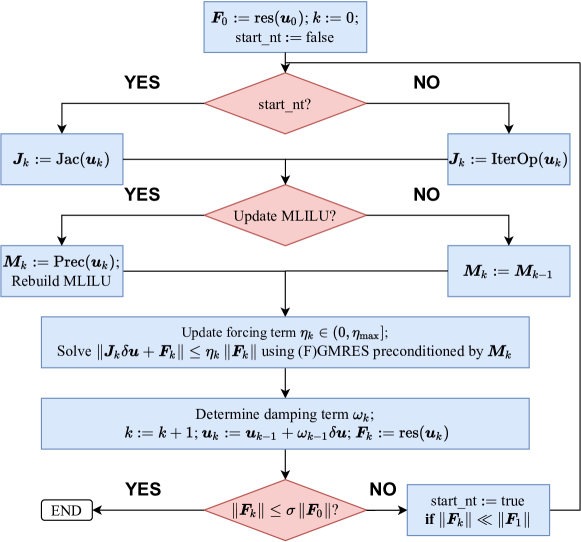
Figure 1: HILUNG algorithm flowchart.

3.1 HILUCSI

The computational kernel of HILUNG is a robust and efficient multilevel ILU preconditioner, called HILUCSI (or Hierarchical Incomplete LU-Crout with Scalability-oriented and Inverse-based dropping), which the authors developed recently.³⁰ HILUCSI shares some similarities with other MLILU (such as ILUPACK³³) in its use of the Crout version of ILU factorization,⁶¹ its dynamic deferring of rows and columns to ensure the well-conditioning of $\tilde{\boldsymbol{B}}$ in (17) at each level,⁵⁴ and its inverse-based dropping for robustness.⁵⁴ Different from ILUPACK, however, HILUCSI improved the robustness for saddle-point problems from PDEs by using static deferring of small diagonals and by utilizing a combination of symmetric and unsymmetric permutations at the top and lower levels, respectively. Furthermore, HILUCSI introduced a scalability-oriented dropping to achieve near-linear time complexity in its factorization and triangular solve. As a result, HILUCSI is particularly well suited for preconditioning large-scale systems arising from INS equations. We refer readers to Chen et al.³⁰ for details of HILUCSI and a comparison with some state-of-the-art ILU preconditioners (including ILUPACK³³ and supernodal ILUTP⁶²) for large-scale indefinite systems.

In the context of preconditioning GMRES for INS, we precondition the Jacobian matrix $\boldsymbol{J}$ (i.e., $\boldsymbol{A}=\boldsymbol{J}$ in (16) and (17)). For efficiency, we apply HILUCSI on a sparsified version of $\boldsymbol{J}$, which we denoted by $\boldsymbol{J}_{S}$ and refer to it as the sparsifying operator (or simply sparsifier). Within Newton iterations, the sparsifier may be the Oseen operator utilizing a previous solution in its linearization. Another potential sparsifier is a lower-order discretization method (see, e.g., Persson and Peraire²¹). The sparsifier is also related to physics-based preconditioners,⁵⁶ except that $\boldsymbol{J}_{S}$ is less restrictive than physics-based preconditioners and hence is easier to construct. In HILUCSI, we note two key parameters in HILUCSI: 1) $\alpha$ for scalability-oriented dropping, which limits the number of nonzeros (nnz) in each column of $\begin{bmatrix}\boldsymbol{L}_{B}\\ \boldsymbol{L}_{E}\end{bmatrix}$ and $\boldsymbol{U}_{F}$ and in each row of $\begin{bmatrix}\boldsymbol{U}_{B}&\boldsymbol{U}_{F}\end{bmatrix}$. 2) droptol, which controls inverse-based dropping. In particular, we limit $\boldsymbol{L}_{E}$ and $\boldsymbol{U}_{F}$ at each level to be within $\alpha$ times the nnz in the corresponding row and column of $\boldsymbol{J}$ subject to a safeguard for rows and columns with a small nnz in $\boldsymbol{J}$. A larger $\alpha$ and a smaller droptol lead to more accurate but also more costly incomplete factors. Hence, we need to balance accuracy and efficiency by adapting these parameters, so that we can achieve robustness while avoiding “over-factorization” in HILUCSI. It is also desirable for the approximation error in the sparsifier (i.e., $\boldsymbol{J}-{\boldsymbol{J}_{S}}$) to be commensurate with the droppings in HILUCSI.

For INS, there is a connection between HILUCSI and the approximate Schur complements, such as PCD and LSC described in Section 2.2. Specifically, HILUCSI defers all small diagonals directly to next level after applying equilibration,⁴⁶ which we refer to as static deferring. At the first level, the static deferring is likely recover the saddle-point structure as in (4) or (5). However, HILUCSI constructs a preconditioner in the form of $\text{$\boldsymbol{M}$}\approx\begin{bmatrix}\tilde{\boldsymbol{B}}&\tilde{\boldsymbol{F}}\\ \tilde{\boldsymbol{E}}&\boldsymbol{C}\end{bmatrix}=\begin{bmatrix}\boldsymbol{L}_{B}&\boldsymbol{0}\\ \boldsymbol{L}_{E}&\boldsymbol{I}\end{bmatrix}\begin{bmatrix}\boldsymbol{D}_{B}&\boldsymbol{0}\\ \boldsymbol{0}&\boldsymbol{S}_{C}\end{bmatrix}\begin{bmatrix}\boldsymbol{U}_{B}&\boldsymbol{U}_{F}\\ \boldsymbol{0}&\boldsymbol{I}\end{bmatrix}$ instead of $\boldsymbol{T}=\begin{bmatrix}\boldsymbol{B}&\boldsymbol{E}^{T}\\ \boldsymbol{0}&\boldsymbol{S}_{T}\end{bmatrix}$ as in PCD and LSC. In other words, HILUCSI preserves more information in the lower-triangular part than approximate Schur complements. In addition, HILUCSI guarantees that $\tilde{\boldsymbol{B}}$ is well-conditioned by dynamically deferring rows and columns to the next level, but $\boldsymbol{B}$ may be ill-conditioned in $\boldsymbol{T}$. For these reasons, we expect HILUCSI to enable faster convergence and deliver better robustness than PCD and LSC, as we will confirm in Section 4. In addition, the implementations of PCD and LSC often rely on complete factorization for its subdomains,^{2, 32} but HILUCSI uses incomplete factorization to obtain $\tilde{\boldsymbol{B}}$ and it factorizes $\boldsymbol{S}_{C}$ recursively. Hence, we expect HILUCSI to deliver better absolute performance per iteration than PCD and LSC. From practical point of view, HILUCSI is also more user-friendly than PCD and LSC, in that it is purely algebraic and does not require the users to modify their PDE codes.

We have previously conducted a thorough analysis of HILUCSI in terms of its accuracy⁶³ and its efficiency.³⁰ In particular, HILUCSI was shown to satisfy an $\epsilon$-accuracy criterion (Definition 3.8 of Jiao and Chen⁶³). As a result, with sufficiently small dropping thresholds, HILUCSI guarantees the convergence of right-preconditioned GMRES, and it converges to an optimal preconditioner as the thresholds decrease, enabling the right-preconditioned GMRES to converge in one iteration at the limit (see Lemma 4.3 and Theorem 3.6 of Jiao and Chen⁶³). Furthermore, the analysis of $\epsilon$-accuracy also applies to singular systems, which is relevant to INS since the Jacobian matrix is singular, with a null space corresponding to the constant mode of the pressure (aka the hydrostatic pressure). In addition, we proved that HILUCSI has (near) linear space and time complexities in its factorization cost and its solve cost per GMRES iteration.³⁰ In contrast, neither the block triangular approximate Schur complement preconditioners² nor the augmented Lagrangian preconditioners^{23, 24} satisfy the $\epsilon$-accuracy criterion, and the complete factorizations typically used for their leading blocks^{31, 32, 26} have superlinear space and time complexity. For these reasons, we expect HILUCSI to perform well as the preconditioner for INS, as we will confirm empirically in Section 4.

3.2 Frequency of factorization

To use HILUCSI effectively as preconditioners in Newton-GMRES, we need to answer two questions: First, how frequently should the sparsifier be recomputed and factorized? Second, how accurate should the incomplete factorization be in terms of $\alpha$ and droptol (cf. Section 2.4)? Clearly, more frequent refactorization and more accurate approximate factorization may improve robustness. However, they may also lower efficiency because factorization (including incomplete factorization) is typically far more expensive than triangular solves. In addition, a more accurate approximate factorization is also denser in general. It is desirable to achieve robustness while minimizing over-factorization. Pernice and Walker¹⁵ used a fixed refactorization frequency to show that it is sometimes advantageous to reuse a previous preconditioner.

Regarding the first question, we recompute and factorize the sparsifier if 1) the number of GMRES iterations in the previous nonlinear step exceeded a user-specified threshold $N$, or 2) the increment in the previous step is greater than some factor of the previous solution vector. The rationale of the first criterion is that an excessive number of GMRES iterations indicates the ineffectiveness of the preconditioner, which is likely due to an outdated sparsifier (assuming the sparsification process and HILUCSI are both sufficiently accurate). The second criterion serves as a safeguard against rapid changes in the solution, especially at the beginning of the nonlinear iterations. Finally, to preserve the quadratic convergence of Newton’s method, we always build a new sparsifier and preconditioner at the first Newton iteration. For the second question, we adapt $\alpha$ and droptol based on whether it is during Picard or Newton iterations. It is desirable to use smaller $\alpha$ and larger droptol during Picard iterations with the Oseen systems for better efficiency and use larger $\alpha$ and smaller droptol for Newton iterations for faster convergence. Based on our numerical experimentation, for low Re ($<200$), we use $\alpha=2$, and we set $\text{droptol}=0.02$ and $0.01$ during Oseen and Newton iterations, respectively. For high Re, we use $\alpha=5$ by default and set $\text{droptol}=0.01$ and $\text{droptol}=0.001$, respectively. It is worth noting that in HILUCSI, the scalability-oriented dropping dominates when droptol is small, and even setting droptol to $0$ for HILUCSI would not lead to excessive fills or loss of near-linear complexity. In contrast, some other ILU techniques, such as ILUTP, would suffer from superlinear complexity and excessive fills when droptol is too small.

3.3 Improving robustness with iterative refinement and null-space elimination

In HILUNG, the sparsification in $\boldsymbol{J}_{S}$, the delay of refactorization, and the droppings in HILUCSI all introduce inaccuracies to the preconditioner $\boldsymbol{M}$. To improve robustness, it may be beneficial to have a built-in correction in $\boldsymbol{M}$. To do this, we utilize the concept of iterative refinement, which is often used in direct solvers for ill-conditioned systems,⁶⁴ and it was also used previously by Dahl and Wille⁶⁵ in conjunction with single-level ILU. With the use of iterative refinement, we utilize the flexible GMRES (FGMRES),⁶⁶ which allows inner iterations within the preconditioner. In our experiments, we found that two inner iterations are enough and can significantly improve the effectiveness of the preconditioner when a sparsifier is used.

In addition, note that the Jacobian matrix may be singular, for example, when the PDE has a pure Neumann boundary condition. We assume the null space is known and project off the null-space components during preconditioning. We refer to it as null-space elimination. In particular, let $\boldsymbol{q}$ be composed of an orthonormal basis of the (right) null space of $\boldsymbol{J}_{k}$. Given a vector $\boldsymbol{v}$ and an intermediate preconditioner $\hat{\boldsymbol{M}}$ obtained from HILUCSI, we construct an “implicit” preconditioner $\boldsymbol{M}$, which computes $\boldsymbol{z}=\boldsymbol{M}^{+}\boldsymbol{\boldsymbol{v}}$ iteratively starting with $\boldsymbol{z}_{0}=\boldsymbol{0}$ and then

$$\boldsymbol{z}_{n}=\boldsymbol{z}_{n-1}+\boldsymbol{\Pi}\hat{\boldsymbol{M}}^{-1}\left(\boldsymbol{\boldsymbol{v}}-\boldsymbol{J}_{k}\boldsymbol{z}_{n-1}\right),\qquad\text{for }n=1,2...,K,$$ (18)

where $\boldsymbol{\Pi}=\boldsymbol{I}-\boldsymbol{q}\boldsymbol{q}^{T}$. If $K=1$, the process results in $\boldsymbol{M}^{+}=\boldsymbol{\Pi}\hat{\boldsymbol{M}}^{-1}$. For large $K$, the process reduces to a stationary iterative solver, which converges when $\rho(\boldsymbol{I}-\boldsymbol{\Pi}\hat{\boldsymbol{M}}^{-1}\boldsymbol{J}_{k})<1$, where $\rho$ denotes the spectral radius. In our experiments, we found that $K=2$ is effective during Newton iterations, which significantly improves efficiency for high Re without compromising efficiency for low Re. Notice that the null-space eliminator $\boldsymbol{\Pi}$ is optional for INS with finite element methods because there exists a constant mode in the pressure with Dirichlet (i.e., fixed velocity) boundary conditions applied to all walls. Moreover, both Eqs. (4) and (5) are range-symmetric, i.e., $\mathcal{N}\left(\boldsymbol{J}_{k}\right)=\mathcal{N}\left(\boldsymbol{J}_{k}^{T}\right)$. Therefore, for (4) and (5), we have both

$$\begin{bmatrix}\boldsymbol{K}+\boldsymbol{C}_{k}+\boldsymbol{W}_{k}&\boldsymbol{E}^{T}\\ \boldsymbol{E}&\boldsymbol{0}\end{bmatrix}\begin{bmatrix}\boldsymbol{0}\\ \boldsymbol{1}\end{bmatrix}=\boldsymbol{0}\qquad\text{and}\qquad\begin{bmatrix}\boldsymbol{K}+\boldsymbol{C}_{k}&\boldsymbol{E}^{T}\\ \boldsymbol{E}&\boldsymbol{0}\end{bmatrix}\begin{bmatrix}\boldsymbol{0}\\ \boldsymbol{1}\end{bmatrix}=\boldsymbol{0},$$ (19)

which means $\boldsymbol{J}_{k}$ can automatically eliminate the null-space component arising from INS. Nevertheless, we observe that such a null-space eliminator can mitigate the effect of round-off errors and reduce the number of iterations.

3.4 Overall algorithm

For completeness, Algorithm 1 presents the pseudocode for HILUNG. The first three arguments of the algorithm, namely $\boldsymbol{F}$, $\boldsymbol{J}$, and $\boldsymbol{x}_{0}$, are similar to typical Newton-like methods. We assume the initial solution $\boldsymbol{x}_{0}$ is obtained from some linearized problems (such as the Stokes equations in the context of INS). Unlike a standard nonlinear solver, HILUNG has a fourth input argument $\boldsymbol{J}_{S}$, which is a callback function. $\boldsymbol{J}_{S}$ returns a matrix, on which we compute the HILUCSI preconditioner $\boldsymbol{M}$; see line 8. To support hot start, HILUNG allows $\boldsymbol{J}$ to return either the Oseen operator (during hot start) or the Jacobian matrix (after hot start); see line 5. The switch from Oseen to Newton iterations is specified in line 4, based on the current residual relative to the initial residual. Line 10 corresponds to the determination of the forcing parameter $\eta_{k}$. During Picard iterations, it is sufficient to use a constant $\eta_{k}$ due to the linear convergence of Picard iterations.² In our tests, we fixed $\eta_{k}$ to be $0.3$. For Newton iterations, we choose $\eta_{k}$ based on the second choice by Eisenstat and Walker;³⁶ specifically, $\eta_{k}=\min\left\{\eta_{\max},0.9\thinspace\left\|\boldsymbol{F}(\boldsymbol{x}_{k})\right\|^{2}/\left\|\boldsymbol{F}(\boldsymbol{x}_{k-1})\right\|^{2}\right\}$, which are further restricted to be no smaller than $0.9\thinspace\eta_{k-1}^{2}$ if $0.9\,\eta_{k-1}^{2}>0.1$.³⁶ To avoid over-solving in the last Newton step, we safeguarded $\eta_{k}$ to be no smaller than $0.5\thinspace\sigma\left\|\boldsymbol{F}\left(\boldsymbol{x}_{0}\right)\right\|/\left\|\boldsymbol{F}\left(\boldsymbol{x}_{k}\right)\right\|$.⁹ Regarding the damping factors, we compute $\omega$ using the Armijo rule by iteratively halving $\omega$, i.e., $\omega_{j}=\omega_{j-1}/2$ for $j=1,2,\ldots,$ with $\omega_{0}\equiv 1$,⁹ as shown between lines 12 and 16.

Algorithm 1 $\boldsymbol{x}=\textrm{{hilung}}\left(\boldsymbol{F},\boldsymbol{J},\boldsymbol{x}_{0},\boldsymbol{J}_{S},\textrm{args}\right)$

$\boldsymbol{F},\boldsymbol{J}$: callback functions for computing residual and Oseen/Jacobian matrix, respectively.

$\boldsymbol{x}_{0}$: initial solution.

$\boldsymbol{J}_{S}$: callback function for computing sparsifying operator (can be same as $\boldsymbol{J}$).

args: control parameters.

1:$\sigma,\eta_{\max},\beta,\epsilon,\alpha,\textrm{droptol},m,N,\theta\leftarrow\text{args}${control parameters}

2:$\boldsymbol{s}_{-1}\leftarrow\boldsymbol{1}$; $\boldsymbol{x}_{-1}\leftarrow\boldsymbol{0}$; $k=0$

3:while $\left\|\boldsymbol{F}\left(\boldsymbol{x}_{k}\right)\right\|>\sigma\left\|\boldsymbol{F}\left(\boldsymbol{x}_{0}\right)\right\|$ do

4:     $\text{started\_nt}\leftarrow\text{$\left\|\boldsymbol{F}\left(\boldsymbol{x}_{k}\right)\right\|$}\leq\beta\left\|\boldsymbol{F}\left(\boldsymbol{x}_{0}\right)\right\|${hot-started Newton if the solution is close}

5:     $\boldsymbol{J}_{k}\leftarrow\boldsymbol{J}\left(\boldsymbol{x}_{k},\textrm{started\_nt}\right)${compute Jacobian/iteration matrix}

6:     if prev. FGMRES iter. count$\geq N$ or $\left\|\boldsymbol{s}_{k-1}\right\|\geq\epsilon\left\|\boldsymbol{x}_{k-1}\right\|$ or first Newton iter. then

7:         adapt $\alpha$ and droptol for HILUCSI based on started_nt

8:         $\boldsymbol{J}_{S,k}\leftarrow\boldsymbol{J}_{S}\left(\boldsymbol{x}_{k},\text{started\_nt}\right)$; construct $\boldsymbol{M}$ from $\boldsymbol{J}_{S,k}$ by factorizing by HILUCSI

9:     end if

10:     determine relative tolerance $\eta_{k}\in\left(0,\eta_{\max}\right]$ based on started_nt for FGMRES($m$)

11:     use FGMRES($m$) to solve $\boldsymbol{J}_{k}\boldsymbol{M}^{-1}\boldsymbol{t}_{k}\approx-\boldsymbol{F}\left(\boldsymbol{x}_{k}\right)$ s.t. $\left\|\boldsymbol{J}_{k}\boldsymbol{s}_{k}+\boldsymbol{F}\left(\boldsymbol{x}_{k}\right)\right\|\leq\eta_{k}\left\|\boldsymbol{F}\left(\boldsymbol{x}_{k}\right)\right\|,\text{ where }\text{$\boldsymbol{s}_{k}=$$\boldsymbol{M}^{-1}\boldsymbol{t}_{k}$}$

12:     $\omega\leftarrow 1${initial damping factor}

13:     while $\left\|\boldsymbol{F}\left(\boldsymbol{x}_{k}+\boldsymbol{s}_{k}\right)\right\|>\left(1-\theta\thinspace\omega\right)\left\|\boldsymbol{F}\left(\boldsymbol{x}_{k}\right)\right\|$ do{we set $\theta=10^{-4}$}

14:         $\omega\leftarrow\omega/2${halve the damping factor}

15:         $\boldsymbol{s}_{k}\leftarrow\omega\thinspace\boldsymbol{s}_{k}$

16:     end while

17:     $\boldsymbol{x}\leftarrow\boldsymbol{x}_{k+1}\leftarrow\boldsymbol{x}_{k}+\boldsymbol{s}_{k}$; $k\leftarrow k+1${update solution and counter}

18:end while

4 Numerical results and comparisons

In this section, we assess the robustness and efficiency of HILUNG. To this end, we compare HILUNG with some of the state-of-the-art customized preconditioners for INS (including two variants of augmented Lagrangian methods^{23, 24, 28, 26} and two “physics-based” preconditioners^{31, 32}) as well as some general-purpose (approximate) factorization techniques (including ILUPACK v2.4³³, MUMPS v5.3.5^{67, 68}, and the popular ILU($k$)^{49, 69}). We solve a 2D stationary INS with Re up to 5000 and a 3D stationary INS with Re 20, with degrees of freedom up to about 2.4 million and 10 million, respectively. When applicable, we discretized the INS equations using $P_{2}$-$P_{1}$ Taylor-Hood (TH) elements⁸ in all the comparisons, which are inf-sup stable.⁷⁰ We used double-precision floating-point arithmetic with a nonlinear residual of $10^{-5}$ or $10^{-6}$. Unless otherwise noted, we used (F)GMRES with restart 30 and limited the maximum number of (F)GMRES iteration to 200 within each nonlinear step. For HILUNG, we set $\epsilon$ to $0.8$ in line 6 to trigger the factorization of $\boldsymbol{J}_{S}$ when the solution changes rapidly, and we set $\beta$ to $0.05$ to switch from Picard iterations to Newton iterations in line 4, while still using the Oseen operator as the sparsifier $\boldsymbol{J}_{S}$ when computing the preconditioner for Newton iterations. We conducted our tests on a single core of a cluster running CentOS 7.4 with dual 2.5 GHz Intel Xeon CPU E5-2680v3 processors and 64 GB of RAM. All compute-intensive kernels in HILUNG were implemented in C++, compiled by GCC 4.8.5 with optimization flag ‘-O3’, and then built into a MEX function for access through MATLAB R2020a with MATLAB’s built-in Intel MKL for LAPACK. We used the same optimization flag and linked them with MKL either with MATLAB’s built-in version (for ILUPACK) with the standalone MKL 2018 (for MUMPS).

4.1 2D driven-cavity problem

We first assess HILUNG using the 2D lid-driven cavity problem over the domain $\left[-1,1\right]^{2}$ using a range of Re and mesh resolutions. This problem is widely used in the literature,^{19, 27, 2} so it allows us to perform quantitative comparisons. The kinetic viscosity is equal to $\nu=2/\text{Re}$. The no-slip wall condition is imposed along all sides except for the top wall. There are two commonly used configurations for the top wall: 1) The standard top wall boundary condition, which reads

$$\boldsymbol{u}_{\text{standard}}=\left[1,0\right],$$ (20)

and 2) a regularized top wall boundary condition, such as²

$$\boldsymbol{u}_{\text{regularized}}=\left[1-x^{4},0\right].$$ (21)

For this comparative study, we considered the standard boundary condition (20), which is more challenging to solve. The pressure field has a “do-nothing” boundary condition, so the coefficient matrix has a null space spanned by $\left[\boldsymbol{0},\boldsymbol{1}\right]^{T}$, where the $\boldsymbol{1}$ components correspond to the constant pressure mode (aka the hydrostatic pressure). We resolved the null space in HILUNG as described in Section 3.3. Despite the simple geometry, the pressure contains two corner singularities (cf. Figure 2b), which become more severe as the mesh is refined, leading to significant challenges for nonlinear solvers and preconditioners. We used uniform meshes following the convention as in Elman et al.,² except that we split the $Q_{2}$ and $Q_{1}$ rectangular elements along one diagonal direction to construct $P_{2}$ and $P_{1}$ triangular elements. We use level-$\ell$ mesh to denote the uniform mesh with $\left(2^{\ell-1}\right)^{2}$ $Q_{2}$ elements. For TH elements, there are $\left(2^{\ell}-1\right)^{2}$ DOFs in velocities and $\left(2^{\ell-1}+1\right)^{2}$ DOFs in pressure. For the level-10 mesh, for example, there are approximately 2.36 million unknowns.

Robustness of HILUNG

We first demonstrate the robustness of HILUNG for $\text{Re}=2000$ and $\text{Re}=5000$, which are moderately high and are challenging due to the corner singularities in pressure (cf. Figure 2b). We chose nonlinear relative tolerance $\sigma=10^{-6}$ in (6), and we used the solution of the Stokes equations as the initial guess for nonlinear iterations in all cases. We set $N=20$ as the threshold to trigger refactorization for the level-8 and 9 meshes, and we reduced it to $N=15$ for the level-10 mesh due to the steeper corner singularities. Figures 2a and 2c plot the velocities along the center lines $x=0$ and $y=0$ and the streamline for $\text{Re}=5000$, which agreed very well with the results of Ghia et al.¹⁹ Figure 3 shows the convergence history of the nonlinear solvers on levels 8, 9, and 10 meshes, along with the total number of GMRES iterations. The results indicate that HILUNG converged fairly smoothly under mesh refinement. It is worth mentioning that no grad-div stabilization was added in HILUNG to its coefficient matrix $\boldsymbol{J}$ or the sparsifier $\boldsymbol{J}_{S}$.

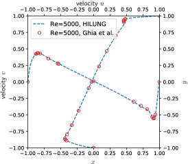
(a) Verification of velocities.

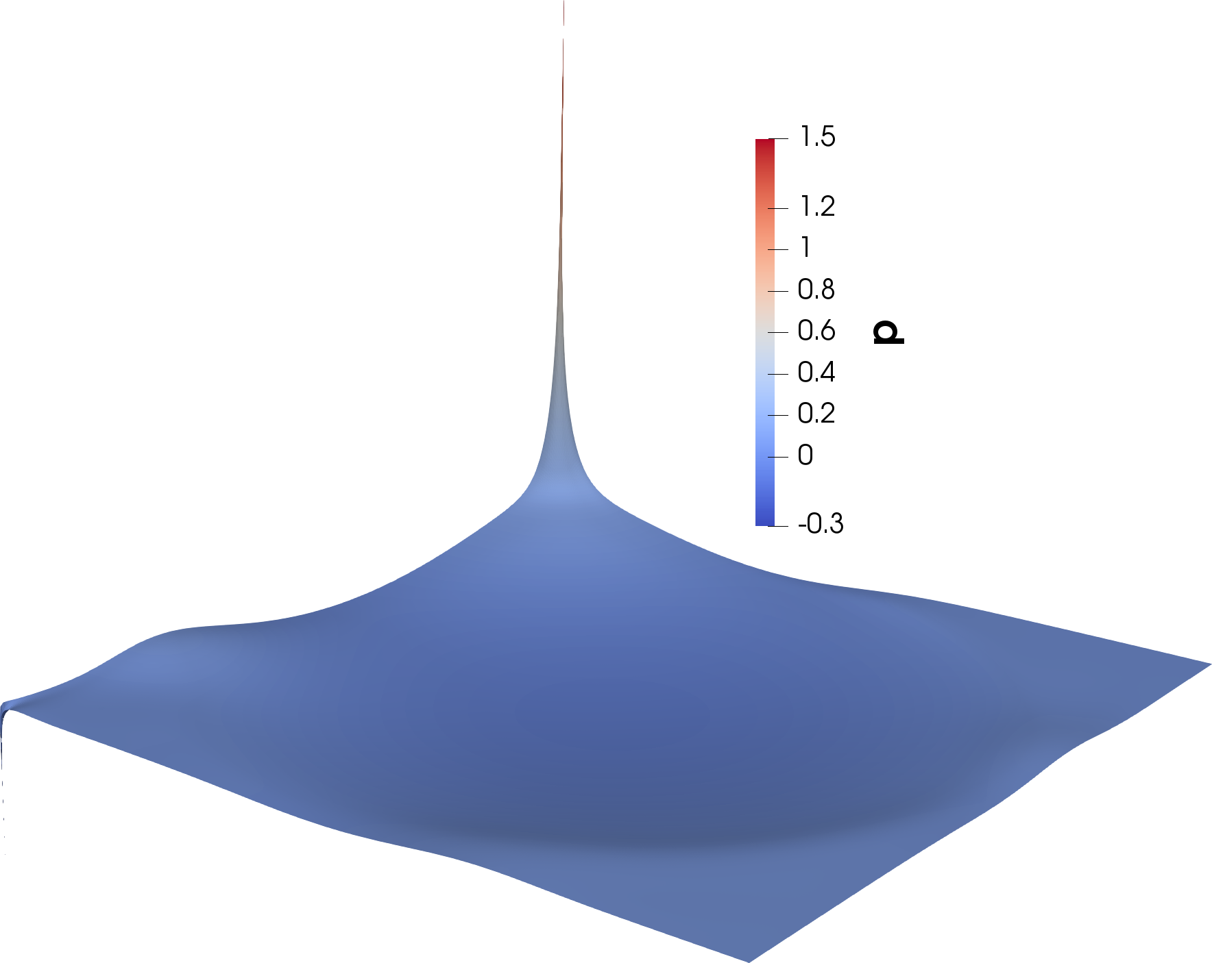
(b) Solution of pressure.

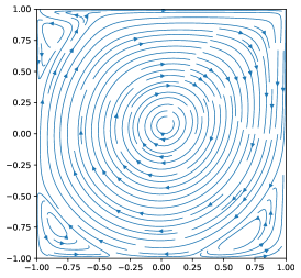
(c) Demonstration of streamline.

Figure 2: 2D driven-cavity problem with standard top-wall boundary condition and Reynolds number $5000$. (a) Comparison of velocities along $x=0$ and $y=0$ with those by Ghia et al.¹⁹ (b) Solutions of pressure with two corner singularities. (c) The streamline plot, which agrees very well to that of Ghia et al.¹⁹

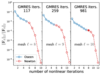
(a) Convergence history of 2D driven-cavity with $\text{Re}=2000$.

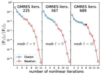
(b) Convergence history of 2D driven-cavity with $\text{Re}=5000$.

Figure 3: Convergence of the 2D driven-cavity problems with different Reynolds numbers (a) 2000 and (b) 5000, where solid dots (i.e., $\CIRCLE$) indicate that damping was invoked.

Effects of adaptive factorization and iterative refinement

We then assess the effectiveness of adaptive refactorization (AR) and iterative refinement (IR) in HILUNG. In our experiments, IR did not improve Picard iterations, so we applied it only to Newton iterations. When IR is enabled, it incurs an extra matrix-vector multiplication. Hence, when IR is disabled, we doubled the upper limit of GMRES iterations per nonlinear solver to 400 and doubled the parameter $N$ to $40$ for triggering refactorization. Table 1 compares the total runtimes and the numbers of GMRES iterations with both AR and IR enabled, with only AR, and with only IR and with refactorization at each each nonlinear iteration. It can be seen that AR was effective in reducing the overall runtimes for all cases because the HILUCSI factorization is more costly than triangular solves. Overall, enabling both AR and IR delivered the best performance, especially on finer meshes. IR was effective on the level-9 mesh. Compared to enabling AR alone, enabling both IR and AR improved runtimes by about 10% for $\text{Re}=1000$ and $2000$ and about 30% for $\text{Re}=5000$.

Table 1: Comparison of total runtimes in seconds and numbers of nonlinear iterations (in parentheses) with both adaptive refactorization (AR) and iterative refinement (IR) (denoted as AR+IR) vs. with only AR and only IR for 2D driven cavity problem with nonlinear relative tolerance $10^{-6}$. Leaders are in boldface.

$\ell$		$\text{Re}=1000$				$\text{Re}=2000$				$\text{Re}=5000$
		AR+IR	AR	IR		AR+IR	AR	IR		AR+IR	AR	IR
7		10.2 (8)	10.9 (8)	16.5 (8)		8.9 (9)	11 (9)	16 (9)		25.8 (15)	38.0 (16)	55.6 (15)
8		55.1 (10)	54.2 (10)	96.2 (10)		46 (10)	49 (10)	91 (10)		146 (12)	213 (13)	194 (12)
9		489 (10)	551 (10)	517 (10)		335 (11)	397 (10)	429 (11)		635 (13)	1.2e3(14)	841 (13)
10		5.2e3 (12)	6.6e3 (16)	5.2e3 (12)		4.3e3 (12)	6.1e3 (17)	4.3e3 (12)		4.2e3 (14)	5.7e3 (16)	4.1e3 (14)

Comparison with customized preconditioners for INS

To evaluate HILUNG with the state-of-the-art customized preconditioners for INS, we compare it with four popular choices, including the augmented Lagrangian (AL) preconditioner as proposed by Benzi and Olshanskii,²³ the modified augmented Lagrangian (MAL) preconditioner as proposed by Benzi, Olshanskii, and Wang,²⁴ the pressure convection diffusion (PCD),^{41, 42} and least-squares commutator (LSC).²⁷ We chose these preconditioners for comparisons since they have all been adopted in some recent open-source software packages,^{3, 28, 25, 32} so they represent the state of the art and we can use the existing software directly for a fair comparison. In particular, for AL, we used ALFI based on FireDrake by Farrell et al.,²⁵ which uses a customized geometric multigrid method for the leading block. For MAL, we used the implementation based on FreeFEM by Moulin et al.,²⁶ hereafter referred to as MAL-FF, which uses the direct solver MUMPS v5.0.2 with OpenBLAS for complete factorization and solve of the leading block. For PCD and LSC, we used the MATLAB implementation in IFISS v3.6,^{31, 32} which uses complete factorization for the leading block. We used the same uniform meshes for HILUNG, ALFI, MAL-FF, and IFISS. However, we used $P_{2}$-$P_{1}$ elements for HILUNG and MAL-FF, used $P_{2}$-$P_{0}$ elements with ALFI,^{25, 28} and used $Q_{2}$-$Q_{1}$ TH elements with IFISS without subdividing the quadrilaterals. This apparent discrepancy is because neither ALFI^{25, 28} nor IFISS supports $P_{2}$-$P_{1}$ TH elements. Although HILUNG could converge to $10^{-6}$ for $\text{Re}=5000$ on the finest mesh, as we have shown in Table 1, we loosened the nonlinear relative tolerance $\sigma$ from $10^{-6}$ to $10^{-5}$ for all the codes, since some other methods had difficulty converging beyond $10^{-5}$ even for smaller Re. Whenever possible, we used the default parameters in IFISS, ALFI, and MAL-FF. It is worth noting that ALFI solved a sequence of problems with different Reynolds numbers (e.g., $\text{Re}=[\text{$\epsilon$},10,100,200,\ldots,5000,\ldots]$ for $\epsilon\approx 0$), and the solution obtained from a smaller Re was used as the initial guess for the next one.²⁵ However, such a ramping would require solving 50 equations before solving for Re=5000, which is overly expensive computationally. Hence, we excluded such a drastic ramping strategy and instead used the solution of the Stokes problem as the initial guess for nonlinear iterations for all the methods, as suggested by Elman et al.² For ALFI, we set the penalty parameter to be $\gamma=10^{4}$, as suggested by Farrell et al.²⁵ For MAL-FF, we used $\gamma=0.3$, since we found that it performed better in our tests than the “optimal” $\gamma\simeq 1$ as suggested by Moulin et al.²⁶ For HILUNG, ALFI, and IFISS, we set the maximum number of (F)GMRES iterations per nonlinear iteration to 200, while preserving its default value of 10000 in MAL-FF to avoid premature termination. Note that IFISS only supports full GMRES (i.e., without restart); for the other codes, we use restarted FGMRES with restart 30.

Table 2 compares the total numbers of GMRES iterations and the numbers of nonlinear iterations for $\text{Re}=200$, $1000$, and $5000$. IFISS failed on all the meshes for $\text{Re}=1000$ and $\text{Re}=5000$, so did MAL-FF for $\text{Re}=5000$, so we omitted them from Table 2. It is evident that HILUNG was the most robust in that it solved all the problems. In contrast, ALFI and MAL-FF had comparable robustness, and PCD and LSC could not solve any of the problems with $\text{Re}\geq 1000$. In terms of the number of GMRES iterations, it can be seen that for $\text{Re}=200$ ALFI and MAL-FF are less sensitive to mesh resolutions than HILUNG. However, ALFI appeared to be more sensitive to mesh resolution than HILUCSI for $\text{Re}=1000$, probably due to the loss of robustness of the customized multigrid solver in ALFI for higher Reynolds number. In contrast, MAL-FF remained insensitive to mesh resolution for $\text{Re}=1000$, probably due to its use of complete factorization of the leading block, whereas HILUCSI uses an incomplete factorization. Nevertheless, HILUNG required fewer numbers of GMRES iterations than ALFI and MAL-FF for $\text{Re}=1000$. More importantly, HILUNG was the only one to solve the problem for $\text{Re}=5000$ on all the meshes. The numbers of GMRES iterations decreased for HILUNG as the meshes refined for $\text{Re}=5000$ up to the level-8 mesh, because the omitted term $\boldsymbol{u}\cdot\boldsymbol{\nabla}\boldsymbol{u}_{k}$ in the sparsifier $\boldsymbol{J}_{S}$ (i.e., the Oseen operator) becomes less and less important as the mesh is refined, so $\boldsymbol{J}_{S}$ becomes better approximations to $\boldsymbol{J}$ as the mesh is refined for high Re.

Table 2: Comparison of the number of nonlinear iterations and total number of GMRES iterations for HILUNG vs. ALFI,^{25, 28} MAL-FF,²⁶ and IFISS v3.6³² with PCD and LSC preconditioners with nonlinear relative tolerance $10^{-5}$. Numbers in parentheses indicate the number of nonlinear iterations. Leaders are in boldface. ‘$\times$’ indicates that the nonlinear solver failed to converge. MAL failed for $\text{Re}=5000$, whereas PCD and LSD failed for $\text{Re}=1000$ and $5000$, so we omit their corresponding columns.

$\ell$		$\text{Re}=200$						$\text{Re}=1000$				$\text{Re}=5000$
		HILUNG	ALFI	MAL-FF	PCD	LSC		HILUNG	ALFI	MAL-FF		HILUNG	AL
6		8 (5)	23 (4)	25 (4)	159 (5)	97 (5)		18 (7)	44 (6)	161 (8)		325 (12)	426 (25)
7		23 (5)	22 (4)	25 (4)	147 (5)	161 (6)		36 (8)	73 (8)	110 (6)		231 (15)	$\times$
8		81 (7)	20 (3)	19 (3)	154 (5)	148 (5)		98 (10)	757 (12)	161 (8)		197 (11)	$\times$

While the number of GMRES iterations is an important measure of the overall efficiency, it is also important to compare the overall computational cost. For completeness, we report detailed timing comparisons for HILUNG, ALFI, and MAL-FF in Table 3. We omit IFISS for timing comparison since it is implemented in MATLAB, it uses full GMRES without restart, and its “ideal setting” uses complete factorization. From Table 3, it is evident that HILUNG is the overall winner in terms of runtime, especially for high Re. In particular, for $\text{Re}=1000$, HILUNG was a factor of two to 40 faster than ALFI and a factor of 1.37–1.75 faster than MAL-FF. Compared to ALFI, the significantly better performance of MAL-FF was probably due to the excellent cache performance of MUMPS for 2D problems. For the same reason, MAL-FF was even faster than HILUNG on the two finer meshes for $\text{Re}=200$. However, as we will show in Section 4.2, MUMPS performs significantly worse for 3D problems due to its increased space and time complexity. For Re=5000, since only HILUNG solved all the problems, only as a point of reference Table 3 reports the runtimes for ALFI and MAL-FF before they reported failures, which took a factor of 4.5 to 40 longer than the successful runs of HILUNG.

Table 3: Comparison of total runtimes in seconds of HILUNG vs. ALFI^{25, 28} and MAL-FF.²⁶ The cases with ‘*’ indicate the runtimes before the code reported failure. Leaders are in boldface.

$\ell$		$\text{Re}=200$				$\text{Re}=1000$				$\text{Re}=5000$
		HILUNG	ALFI	MAL-FF		HILUNG	ALFI	MAL-FF		HILUNG	ALFI	MAL-FF
6		1.39	3.0	1.64		2.13	4.23	3.74		7.21	32.6	75.2*
7		7.95	14.0	6.9		8.42	37.8	11.6		25.6	813*	281*
8		40.8	59.4	25.1		41.9	1.7e3	67.6		124	4.4e4*	1.2e3*

In this 2D comparison, the superior robustness and efficiency of HILUNG were primarily due to the use of HILUCSI as its preconditioner, which enabled robust convergence of GMRES in the inner iteration. This conclusion is supported by the study, since almost all the methods had a comparable number of nonlinear iterations, and the main differences are the average numbers of GMRES iterations. Furthermore, MAL-FF failed for $\text{Re}=5000$ due to the lack of convergence of GMRES in its inner iteration, even when its maximum number of GMRES iterations was set to 10000, probably due to its poor approximation to the Schur complement with a small $\gamma$; similarly, IFISS also seems to suffer from an inaccurate approximation to the Schur complement, even for $\text{Re}=1000$, despite its use of complete factorization and full GMRES. For ALFI, GMRES also converged slowly on finer meshes for higher Re, probably because the large grad-div penalty term $\gamma\boldsymbol{\nabla}\boldsymbol{\nabla}\cdot\boldsymbol{u}$ with $\gamma=10^{4}$ in AL led to ill-conditioning of the overall system, making it difficult for the pressure to converge, especially near the corner singularities. HILUCSI does not suffer from any of these deficiencies, although its scalability is not as good as a multigrid method for low Re.

4.2 3D laminar flow over cylinder

Since real-world fluid problems are typically 3D, we also assess HILUNG for a 3D problem, namely the flow-over-cylinder problem described by Schäfer and Turek.⁷¹ The computation domain is shown in Figure 4a. The inflow (front face) reads $\boldsymbol{u}=\left[U(y,z),0,0\right]^{T}$ with $U(y,z)=16\times 0.45\thinspace yz\left(H-y\right)\left(H-z\right)/H^{4}$, where $H=0.41$ is the height and width of the channel. A “do-nothing” velocity is imposed for the outflow along with zero pressure. The no-slip wall condition is imposed on the top, bottom, and cylinder faces. The Reynolds number of this problem is given by $\text{Re}=4\times 0.45\thinspace D/(9\thinspace\nu)=20$, where $D=0.1$ and $\nu=1\times 10^{-3}$ are the cylinder diameter and kinetic viscosity, respectively. We generated four tetrahedral meshes of different resolutions using Gmsh.⁷² Despite small Re, the small viscosity leads to strongly asymmetric and indefinite Jacobian matrices, making it difficult for Newton’s method to converge. Table 4 shows the statistics of the matrices, where the largest system has about $10$ million DOFs and $907$ million nonzeros. Due to the global convergence property of Picard iterations with the Oseen systems² Chpt. 8 and their use to hot start Newton’s method in HILUNG, HILUNG converges robustly for this problem on all the meshes. Figure 4b shows a sample mesh and the fluid speed computed using HILUNG.

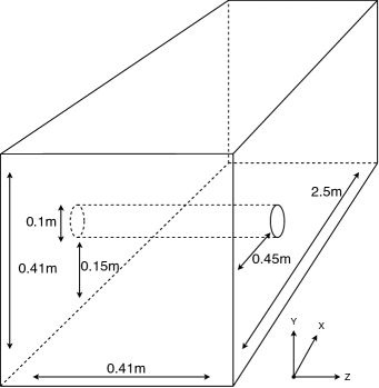
(a) Computational domain.

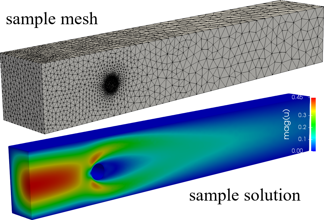
(b) Example graded coarse mesh (top) and the computed fluid speed (bottom).

Figure 4: Computational domain (a) and sample mesh and solution (b) of 3D flow-over-cylinder problem. The front and back faces correspond to the inflow and outflow walls, respectively.

Table 4: Statistics of different levels of meshes for 3D flow, where nnz_J and nnz_S indicate number of nonzeros in Newton and Oseen operators, respectively.

		mesh 1	mesh 2	mesh 3	mesh 4
#elems		71,031	268,814	930,248	2,415,063
#unkowns		262,912	1,086,263	3,738,327	9,759,495
nnz_J		21,870,739	98,205,997	343,357,455	906,853,456
nnz_S		9,902,533	43,686,979	152,438,721	401,879,584

Efficiency comparison with other general-purpose approximate factorizations

For the comparative study of the 2D problem in Section 4.1, the use of HILUCSI was the major factor for the robustness and efficiency of HILUNG. Since HILUCSI is a general-purpose approximate factorization, we focus on comparing HILUCSI with other general-purpose approximate factorizations for this 3D comparative study, including ILUPACK v2.4,⁷³ and single-precision MUMPS v5.3.5.^{67, 68} ILUPACK is most related to HILUCSI in that it also uses multilevel ILU. In both HILUCSI and ILUPACK, we used droptol $0.02$ and $0.01$ during Picard and Newton iterations, respectively, and used their respective default options for the other parameters. To be comparable with single-precision MUMPS, we also enabled mixed-precision computations in both HILUCSI and ILUPACK. For completeness, we also included ILU($1$) and ILU($2$) in our comparison due to its popularity.^{49, 69} Since none of these preconditioners has a corresponding nonlinear solver, for a fair comparison, we used the same nonlinear solver as described in Algorithm 1 and simply replaced HILUCSI with these approximate-factorization techniques as the preconditioner for GMRES. In particular, we used GMRES(30) in the inner iteration and used relative tolerance of $10^{-6}$ for the nonlinear iteration.

Table 5 reports the factorization times, total runtimes, and the numbers of nonlinear and GMRES iterations for the four meshes. Table 5 shows that nonlinear solver failed to converge for any of the meshes for GMRES with ILU($1$) and ILU(2), even after applying equilibration⁴⁶ and fill-reduction reordering⁴⁷ to improve its robustness, despite the global convergence property of Picard iterations with the Oseen systems and hot-started Newton iterations. For the two coarser meshes, compared to ILUPACK, HILUCSI was about a factor of 10 and 34 faster in terms of factorization cost and a factor of 3.4 and 6.6 faster overall. MUMPS under-performed HILUCSI in terms of both factorization and overall times, although it reduced the number of GMRES iterations. In addition, we also tested the multi-threaded MUMPS on 24 cores, which also under-performed the serial HILUCSI by a factor of 1.4–1.7 in the overall runtimes for the two coarser meshes due to the poor speedup of triangular solves, which dominate the overall runtimes.

Table 5: Comparison of factorization times, total times, and the number of GMRES and nonlinear iterations for approximate-factorization-based preconditioners for the 3D flow-over-cylinder problem. ‘$\times$’ indicates nonconvergence of nonlinear iterations with ILU(1) and ILU(2), and ‘$-$’ indicates that factorization ran out of the 64GB main memory. Numbers in the parentheses indicate the number of nonlinear iterations. Leaders are in boldface.

prec.		factorization times (s)					total times (s)					GMRES and Newton iters.
		mesh 1	mesh 2	mesh 3	mesh 4		mesh 1	mesh 2	mesh 3	mesh 4		mesh 1	mesh 2	mesh 3	mesh 4
HILUCSI		17.5	78.3	255	659		71.5	485	1.8e3	4.2e3		135 (10)	200 (13)	199 (11)	249 (11)
ILU(1) or (2)		$\times$	$\times$	$\times$	$\times$		$\times$	$\times$	$\times$	$\times$		$\times$	$\times$	$\times$	$\times$
ILUPACK		182	2.7e3	$-$	$-$		246	3.2e3	$-$	$-$		128 (9)	150 (11)	$-$	$-$
MUMPS		39.3	649	$-$	$-$		95.8	1.5e3	$-$	$-$		89 (10)	127 (11)	$-$	$-$

Comparison of space and time complexities

It is worth noting that both ILUPACK and single-precision MUMPS ran out of the main 64 GB memory for the two larger meshes despite the use of a sparsifier. If HILUCSI were applied to the full Jacobian matrix for Newton’s iterations, HILUNG would have also run out of memory for the largest system. However, a more fundamental reason for ILUPACK and MUMPS to run out of memory was that they both appear to have superlinear space complexities, in that the number of nonzeros in the (approximate) triangular factors grow super-linearly for ILUPACK and MUMPS, as evident in Figure 5a, which shows the growth of nonzeros in the factorization of the Oseen operator for HILUCSI, ILUPACK, and MUMPS, with $\text{droptol}=0.02$ for both HILUCSI and ILUPACK. The superlinear space complexity also implies that the factorization costs of ILUPACK and MUMPS are superlinear, as evident in Figure 5b. Such a superlinear complexity limits the scalability of ILUPACK and MUMPS to large-scale problems, even for the parallel version of MUMPS, regardless of whether sparsifiers are used. In contrast, HILUCSI scaled linearly in both memory and computational cost for its factorization and solve steps, thanks to its scalability-oriented dropping in its multilevel structure.

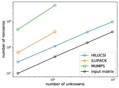
(a) Space complexity.

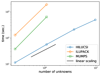
(b) Time complexity.

Figure 5: Comparison of (a) space and (b) time complexities of approximate factorizations.

5 Conclusions

In this work, we introduced HILUNG, which is the first to incorporate a robust multilevel ILU preconditioner into Newton-GMRES to solve the nonlinear equations from incompressible Navier-Stokes equations. In particular, HILUNG applies HILUCSI on a physics-aware sparsifying operator to compute a multilevel ILU. Thanks to the scalability-oriented and inverse-based dual thresholding in HILUCSI, HILUNG enjoys robust and rapid convergence of restarted GMRES in its inner loops. Furthermore, by utilizing adaptive refactorization and iterative refinement to improve runtime efficiency and leverages some standard nonlinear techniques (including hot starting and damping), HILUNG achieved high robustness and efficiency without suffering from potential over-factorization. We demonstrated the effectiveness of HILUNG for stationary incompressible Navier-Stokes equations using Taylor-Hood elements. In addition, we compared HILUNG with some state-of-the-art customized preconditioners, including two variants of augmented Lagrangian preconditioners and two physics-based preconditioners, for the 2D driven-cavity problem with the standard top-wall boundary condition. We showed that HILUNG was the most robust in solving the problem with Re $5000$ successfully on all levels of meshes and was also the most efficient for Re $1000$. In addition, we demonstrated HILUNG in solving the 3D flow-over-cylinder problem with ten million DOFs using only 60GB of RAM, while other alternatives failed to solve the problem on the same system with less than four million DOFs. We also showed that HILUNG outperformed another state-of-the-art multilevel ILU preconditioner by more than an order of magnitude for a system with one million DOFs, and even outperformed a state-of-the-art parallel direct solver on 24 cores for the same system. We have released the source code of HILUCSI as part of the HIFIR project at https://github.com/hifirworks/hifir. One limitation of this work is that HILUCSI is only serial. Future research directions include parallelizing HILUCSI, applying it to solve even higher-Re and larger-scale problems, and developing a custom preconditioner for time-dependent INS with fully implicit Runge-Kutta schemes.

Data availability statement

The core component of HILUNG, HILUCSI, is available as part of an open-source library HIFIR at https://github.com/hifirworks/hifir. Additional data that support the findings of this study are available from the corresponding author upon reasonable request.

References

- 1 Turek S. A comparative study of time-stepping techniques for the incompressible Navier–Stokes equations: from fully implicit non-linear schemes to semi-implicit projection methods. Int. J. Numer. Methods Fluids 1996; 22(10): 987–1011.
- 2 Elman HC, Silvester DJ, Wathen AJ. Finite Elements and Fast Iterative Solvers: With Applications In Incompressible Fluid Dynamics. Oxford University Press, USA. 2nd ed. 2014.
- 3 Bootland N, Bentley A, Kees C, Wathen A. Preconditioners for two-phase incompressible Navier–Stokes flow. SIAM J. Sci. Comput. 2019; 41(4): B843–B869.
- 4 Pearson JW, Pestana J. Preconditioners for Krylov subspace methods: An overview. GAMM-Mitteilungen 2020; 43(4): e202000015.
- 5 Pernice M, Tocci MD. A multigrid-preconditioned Newton–Krylov method for the incompressible Navier–Stokes equations. SIAM J. Sci. Comput. 2001; 23(2): 398–418.
- 6 Heath MT. Scientific Computing: An Introductory Survey. 80. SIAM . 2018.
- 7 Brown PN, Saad Y. Convergence theory of nonlinear Newton–Krylov algorithms. SIAM J. Optim. 1994; 4(2): 297–330.
- 8 Taylor C, Hood P. A numerical solution of the Navier–Stokes equations using the finite element technique. Comput. Fluids 1973; 1(1): 73–100.
- 9 Kelley CT. Iterative Methods for Linear and Nonlinear Equations. 16. SIAM . 1995.
- 10 Benzi M, Golub GH, Liesen J. Numerical solution of saddle point problems. Acta Numerica 2005; 14: 1–137.
- 11 Brown PN, Saad Y. Hybrid Krylov methods for nonlinear systems of equations. SIAM J. Sci. Comput. 1990; 11(3): 450–481.
- 12 Knoll DA, Keyes DE. Jacobian-free Newton–Krylov methods: a survey of approaches and applications. J. Comput. Phys. 2004; 193(2): 357–397.
- 13 Qin N, Ludlow DK, Shaw ST. A matrix-free preconditioned Newton/GMRES method for unsteady Navier–Stokes solutions. Int. J. Numer. Methods Fluids 2000; 33(2): 223–248.
- 14 Saad Y. Iterative Methods for Sparse Linear Systems. 82. SIAM. 2nd ed. 2003.
- 15 Pernice M, Walker HF. NITSOL: A Newton iterative solver for nonlinear systems. SIAM J. Sci. Comput. 1998; 19(1): 302–318.
- 16 Gaston D, Newman C, Hansen G, Lebrun-Grandie D. MOOSE: A parallel computational framework for coupled systems of nonlinear equations. Nucl. Eng. Des. 2009; 239(10): 1768–1778.
- 17 Brune PR, Knepley MG, Smith BF, Tu X. Composing scalable nonlinear algebraic solvers. SIAM Rev. 2015; 57(4): 535–565.
- 18 Balay S, Abhyankar S, Adams M, et al. PETSc Users Manual. Argonne National Laboratory; Argonne, IL: 2019.
- 19 Ghia U, Ghia KN, Shin C. High-Re solutions for incompressible flow using the Navier–Stokes equations and a multigrid method. J. Comput. Phys. 1982; 48(3): 387–411.
- 20 Tuminaro RS, Walker HF, Shadid JN. On backtracking failure in Newton–GMRES methods with a demonstration for the Navier–Stokes equations. J. Comput. Phy. 2002; 180(2): 549–558.
- 21 Persson PO, Peraire J. Newton–GMRES preconditioning for discontinuous Galerkin discretizations of the Navier–Stokes equations. SIAM J. Sci. Comput. 2008; 30(6): 2709–2733.
- 22 ur Rehman M, Vuik C, Segal G. A comparison of preconditioners for incompressible Navier–Stokes solvers. Int. J. Numer. Methods Fluids 2008; 57(12): 1731–1751.
- 23 Benzi M, Olshanskii MA. An augmented Lagrangian-based approach to the Oseen problem. SIAM J. Sci. Comput. 2006; 28(6): 2095–2113.
- 24 Benzi M, Olshanskii MA, Wang Z. Modified augmented Lagrangian preconditioners for the incompressible Navier–Stokes equations. Int. J. Numer. Methods Fluids 2011; 66(4): 486–508.
- 25 Farrell PE, Mitchell L, Wechsung F. An Augmented Lagrangian Preconditioner for the 3D Stationary Incompressible Navier–Stokes Equations at High Reynolds Number. SIAM J. Sci. Comput. 2019; 41(5): A3073–A3096.
- 26 Moulin J, Jolivet P, Marquet O. Augmented Lagrangian preconditioner for large-scale hydrodynamic stability analysis. Comput. Methods Appl. Mech. Eng. 2019; 351: 718–743.
- 27 Elman H, Howle VE, Shadid J, Shuttleworth R, Tuminaro R. Block preconditioners based on approximate commutators. SIAM J. Sci. Comput. 2006; 27(5): 1651–1668.
- 28 Software used in "An augmented Lagrangian preconditioner for the 3D stationary incompressible Navier–Stokes equations at high Reynolds number". https://doi.org/10.5281/zenodo.3247427; 2019
- 29 Lee M, Moser RD. Direct numerical simulation of turbulent channel flow up to . J. Fluid Mech. 2015; 774: 395–415.
- 30 Chen Q, Ghai A, Jiao X. HILUCSI: Simple, robust, and fast multilevel ILU for large-scale saddle-point problems from PDEs. Numer. Linear Algebra Appl. 2021. doi: 10.1002/nla.2400
- 31 Elman H, Ramage A, Silvester D. IFISS: A computational laboratory for investigating incompressible flow problems. SIAM Rev. 2014; 56: 261–273.
- 32 Silvester D, Elman H, Ramage A. Incompressible Flow and Iterative Solver Software (IFISS) version 3.5. http://www.manchester.ac.uk/ifiss; 2016.
- 33 Bollhöfer M, Aliaga JI, Martín AF, Quintana-Ortí ES. ILUPACK. Encyclopedia of Parallel Computing 2011: 917–926.
- 34 Dembo RS, Eisenstat SC, Steihaug T. Inexact Newton methods. SIAM J. Numer. Anal. 1982; 19(2): 400–408.
- 35 Eisenstat SC, Walker HF. Globally convergent inexact Newton methods. SIAM J. Optim. 1994; 4(2): 393–422.
- 36 Eisenstat SC, Walker HF. Choosing the forcing terms in an inexact Newton method. SIAM J. Sci. Comput. 1996; 17(1): 16–32.
- 37 Dennis Jr JE, Schnabel RB. Numerical Methods for Unconstrained Optimization and Nonlinear Equations. 16. SIAM . 1996.
- 38 An HB, Bai ZZ. A globally convergent Newton–GMRES method for large sparse systems of nonlinear equations. Appl. Numer. Math 2007; 57(3): 235–252.
- 39 Bellavia S, Morini B. A globally convergent Newton-GMRES subspace method for systems of nonlinear equations. SIAM J. Sci. Comput. 2001; 23(3): 940–960.
- 40 Murphy MF, Golub GH, Wathen AJ. A note on preconditioning for indefinite linear systems. SIAM J. Sci. Comput. 2000; 21(6): 1969–1972.
- 41 Silvester D, Elman H, Kay D, Wathen A. Efficient preconditioning of the linearized Navier–Stokes equations for incompressible flow. J. Comput. Appl. Math. 2001; 128(1-2): 261–279.
- 42 Kay D, Loghin D, Wathen A. A preconditioner for the steady-state Navier–Stokes equations. SIAM J. Sci. Comput. 2002; 24(1): 237–256.
- 43 Fortin M, Glowinski R. Augmented Lagrangian Methods: Applications to the Numerical Solution of Boundary-Value Problems. Elsevier . 2000.
- 44 He X, Vuik C. Efficient and robust Schur complement approximations in the augmented Lagrangian preconditioner for the incompressible laminar flows. J. Comput. Phys. 2020; 408: 109286.
- 45 Nocedal J, Wright S. Numerical Optimization. Springer Science & Business Media . 2006.
- 46 Duff IS, Koster J. On algorithms for permuting large entries to the diagonal of a sparse matrix. SIAM J. Matrix Anal. Appl. 2001; 22(4): 973–996.
- 47 Amestoy PR, Davis TA, Duff IS. An approximate minimum degree ordering algorithm. SIAM J. Matrix Anal. Appl. 1996; 17(4): 886–905.
- 48 Saad Y. Preconditioning techniques for nonsymmetric and indefinite linear systems. J. Comput. Appl. Math. 1988; 24(1-2): 89–105.
- 49 Yang C, Cai XC. A scalable fully implicit compressible Euler solver for mesoscale nonhydrostatic simulation of atmospheric flows. SIAM J. Sci. Comput. 2014; 36(5): S23–S47.
- 50 Saad Y. ILUT: A dual threshold incomplete LU factorization. Numer. Linear Algebra Appl. 1994; 1(4): 387–402.
- 51 Saad Y. Multilevel ILU with reorderings for diagonal dominance. SIAM J. Sci. Comput. 2005; 27(3): 1032–1057.
- 52 Konshin I, Olshanskii M, Vassilevski Y. LU factorizations and ILU preconditioning for stabilized discretizations of incompressible Navier–Stokes equations. Numer. Linear Algebra Appl. 2017; 24(3): e2085.
- 53 Mayer J. A multilevel Crout ILU preconditioner with pivoting and row permutation. Numer. Linear Algebra Appl. 2007; 14(10): 771–789.
- 54 Bollhöfer M, Saad Y. Multilevel preconditioners constructed from inverse-based ILUs. SIAM J. Sci. Comput. 2006; 27(5): 1627–1650.
- 55 Ghai A, Lu C, Jiao X. A comparison of preconditioned Krylov subspace methods for large-scale nonsymmetric linear systems. Numer. Linear Algebra Appl. 2017; 26: e2215.
- 56 Elman H, Howle VE, Shadid J, Shuttleworth R, Tuminaro R. A taxonomy and comparison of parallel block multi-level preconditioners for the incompressible Navier–Stokes equations. J. Comput. Phy. 2008; 227(3): 1790–1808.
- 57 Briggs WL, Henson VE, McCormick SF. A Multigrid Tutorial. 72. SIAM. 2nd ed. 2000.
- 58 Lu C, Jiao X, Missirlis N. A hybrid geometric+ algebraic multigrid method with semi-iterative smoothers. Numer. Linear Algebra Appl. 2014; 21(2): 221–238.
- 59 Rudi J, Malossi ACI, Isaac T, et al. An extreme-scale implicit solver for complex PDEs: highly heterogeneous flow in earth’s mantle. In: Proceedings of the International Conference for High Performance Computing, Networking, Storage and Analysis. ACM. ; 2015: 5.
- 60 Elman HC, Howle VE, Shadid JN, Tuminaro RS. A parallel block multi-level preconditioner for the 3D incompressible Navier–Stokes equations. J. Comput. Phy. 2003; 187(2): 504–523.
- 61 Li N, Saad Y, Chow E. Crout versions of ILU for general sparse matrices. SIAM J. Sci. Comput. 2003; 25(2): 716–728.
- 62 Li XS, Shao M. A supernodal approach to incomplete LU factorization with partial pivoting. ACM Trans. Math. Softw. 2011; 37(4): 43.
- 63 Jiao X, Chen Q. Approximate generalized inverses with iterative refinement for -accurate preconditioning of singular systems. arxiv 2020. arXiv:2009.01673.
- 64 Golub GH, Van Loan CF. Matrix Computations. Johns Hopkins. 4th ed. 2013.
- 65 Dahl O, Wille S. An ILU preconditioner with coupled node fill-in for iterative solution of the mixed finite element formulation of the 2D and 3D Navier–Stokes equations. Int. J. Numer. Methods Fluids 1992; 15(5): 525–544.
- 66 Saad Y. A flexible inner-outer preconditioned GMRES algorithm. SIAM J. Sci. Comput. 1993; 14(2): 461–469.
- 67 Amestoy PR, Duff IS, L’Excellent JY, Koster J. MUMPS: a general purpose distributed memory sparse solver. In: International Workshop on Applied Parallel Computing. Springer. ; 2000: 121–130.
- 68 Amestoy P, Buttari A, L’Excellent JY, Mary T. Performance and Scalability of the Block Low-Rank Multifrontal Factorization on Multicore Architectures. ACM Trans. Math. Software 2019; 45: 2:1–2:26.
- 69 Miller K. ILU() preconditioner. https://www.mathworks.com/matlabcentral/fileexchange/48320-ilu-k-preconditioner, MATLAB File Exchange; 2019. Retrieved December 15, 2019.
- 70 Boffi D, Brezzi F, Fortin M, others . Mixed Finite Element Methods and Applications. 44. Springer . 2013.
- 71 Schäfer M, Turek S, Durst F, Krause E, Rannacher R. Benchmark computations of laminar flow around a cylinder. In: Flow Simulation with High-Performance Computers II. Springer. 1996 (pp. 547–566).
- 72 Geuzaine C, Remacle JF. Gmsh: A 3-D finite element mesh generator with built-in pre-and post-processing facilities. Int. J. Numer. Meth. Eng. 2009; 79(11): 1309–1331.
- 73 Bollhöfer M, Saad Y, Schenk O. ILUPACK-preconditioning software package. Available online at the URL: http://ilupack.tu-bs.de 2006.