Few-shot Object Grounding and Mapping
for Natural Language Robot Instruction Following

Abstract

We study the problem of learning a robot policy to follow natural language instructions that can be easily extended to reason about new objects. We introduce a few-shot language-conditioned object grounding method trained from augmented reality data that uses exemplars to identify objects and align them to their mentions in instructions. We present a learned map representation that encodes object locations and their instructed use, and construct it from our few-shot grounding output. We integrate this mapping approach into an instruction-following policy, thereby allowing it to reason about previously unseen objects at test-time by simply adding exemplars. We evaluate on the task of learning to map raw observations and instructions to continuous control of a physical quadcopter. Our approach significantly outperforms the prior state of the art in the presence of new objects, even when the prior approach observes all objects during training.

Keywords: language grounding; uav; vision and language; few-shot learning;

1 Introduction

Executing natural language instructions with robotic agents requires addressing a diverse set of problems, including language understanding, perception, planning, and control. Most commonly, such systems are a combination of separately built modules [e.g., 1, 2, 3, 4, 5]. Beyond the high engineering and integration costs of such a system, extending it, for example to reason about new object types, demands complex updates across multiple modules. This is also challenging in recent representation learning approaches, which learn to directly map raw observations and instructions to continuous control [6]. Learned representations entangle different aspects of the problem, making it challenging to extend model reasoning without re-training on additional data.

This paper makes two general contributions. First, we propose a few-shot method to ground natural language object mentions to their observations in the world. Second, we design a process to construct an object-centric learned map from groundings of object mentions within instructions. We show the effectiveness of this map for instruction following by integrating it into an existing policy design to map from raw observations to continuous control. The policy’s few-shot grounding process allows it to reason about previously unseen objects without requiring any additional fine-tuning or training data. The system explicitly reasons about objects and object references, while retaining the reduction in representation design and engineering that motivates learning approaches for language grounding.

Figure 1 illustrates our approach. Rather than learning to implicitly ground instructions inside an opaque neural network model, our few-shot grounding method learns to align natural language mentions within instructions to objects in the environment using a database, which includes exemplars of object appearances and names. This does not require modeling specific objects or object types, but instead relies on learning generic object properties and language similarity. The system’s abilities are easily extended to reason about new objects by extending the database. For example, a user teaching a robot about a new object can simply take a few photos of the object and describe it. In contrast to existing approaches [e.g., 1, 2, 4, 6], ours does not require additional instruction data, training, tuning, or engineering to follow instructions that mention the new object.

We train the object grounding component to recognize objects using a large augmented reality (AR) dataset of synthetic 3D objects automatically overlaid on environment images. This data is cheap to create, and its scale enables the model to generalize beyond the properties of any specific object. We train the complete policy to map instructions and inferred alignments to continuous control in a simulation. Because we learn to reason about object appearance in the real environment using AR data, we can immediately deploy the model for flight in the physical environment by swapping the object grounding component from one trained on simulator-based AR data to one trained on real-world AR data, without any domain adaptation or training in the real world.

Figure 1: Task and approach illustration, including a third-person view of the environment (unavailable to the agent), an agent’s first-person RGB observation, a natural language instruction, and an object database. The agent’s reasoning can be extended by adding entries to the database.

We evaluate on a physical quadcopter situated in an environment that contains only previously unseen objects. The only information available about each object is a handful of images and descriptive noun phrases. Our approach’s object-centric generalization stands in contrast to symbolic methods that typically require anticipating the full set of objects, or representation learning methods that require training data with similar objects. Our few-shot policy outperforms the existing state of the art by 27% absolute improvement in terms of human evaluation scores, and even outperforms a model that has seen the full set of objects during training by 10%. Code and videos are available at https://github.com/lil-lab/drif/tree/fewshot2020.

2 Related Work

Natural language instruction following on physical robots is most commonly studied using hand-engineered symbolic representations of world state or instruction semantics [1, 7, 2, 3, 4, 8, 5, 9], which require representation design and state estimation pipelines that are hard to scale to complex environments. Recently, representation learning based on deep neural networks has been used for this task by mapping raw first-person observations and pose estimates to continuous control [6]. Prior, representation learning was studied on language tasks restricted to simulated discrete [10, 11, 12, 13, 14, 15] and continuous [16, 17, 18, 19] environments, or non-language robotic tasks [20, 21, 22, 23].

Representation learning reduces the engineering effort, but results in models that are difficult to extend. For example, the PVN2 model by Blukis et al. [6] is evaluated in environments that consist of 63 different objects, all seen by the model during training. As we show in Section 8, PVN2 fails to handle new objects during test time. Other work has shown generalization to new indoor scenes [24, 12, 25], but not to objects not represented in the training set. In contrast, our representation learning approach enables deployment in environments with new objects not seen before during training, without any additional instruction data. We use the two-stage model decomposition, SuReAL training algorithm, and map projection mechanism from Blukis et al. [26, 6], but completely re-design the perception, language understanding, grounding, and mapping mechanisms. Our system contribution is a robot representation learning system that follows natural language instructions with easily extensible reasoning capabilities. To the best of our knowledge, no existing approach provides this.

Rather than relying on new training data, we use an extensible database of visual and linguistic exemplars in a few-shot setup. At the core of our approach is a few-shot language-conditioned segmentation component. This mechanism is related to Prototypical Networks [27], but integrates both vision and language modalities. Vision-only few-shot learning has been studied extensively for classification [e.g., 28, 29, 27] and segmentation [30]. Our language-conditioned segmentation problem is a variant of referring expression recognition [31, 32, 33, 34, 35]. Our method is related to a recent alignment-based approach to referring expression resolution using an object database [31].

3 Technical Overview

Our focus is reasoning about objects not seen during training. This overview places our work in the context of the complete system. We adopt the task setup, policy decomposition, and parts of the learning process from Blukis et al. [6], and borrow parts of the overview for consistency.

Task Setup

Our goal is to map natural language navigation instructions to continuous control of a quadcopter drone. The agent behavior is determined by a velocity controller setpoint $\rho=(v,\omega)$, where $v\in\mathds{R}$ is a forward velocity and $\omega\in\mathds{R}$ is a yaw rate. The model generates actions at fixed intervals. An action is either the task completion action ${\tt STOP}$ or a setpoint update $(v,\omega)\in\mathds{R}^{2}$. Given a setpoint update $a_{t}=(v_{t},\omega_{t})$ at time $t$, we set the controller setpoint $\rho=(v_{t},\omega_{t})$ that is maintained between actions. Given a start state $s_{1}$ and an instruction $u$, an execution $\Xi$ of length $T$ is a sequence $\langle(s_{1},a_{1}),\dots,(s_{T},a_{T})\rangle$, where $s_{t}$ is the state at time $t$, $a_{t<T}\in\mathds{R}^{2}$ are setpoint updates, and $a_{T}={\tt STOP}$. The agent has access to raw first-person monocular observations and pose estimates, and does not have access to the world state. The agent also has access to an object database $\mathcal{O}=\{o^{(1)},\ldots,o^{(k)}\}$, where each object $o^{(i)}=(\{Q_{1}^{(i)},\ldots,Q_{q}^{(i)}\},\{W_{1}^{(i)},\ldots,W_{w}^{(i)}\})$ is represented by sets of images $Q_{j}^{(i)}$ and natural language descriptions $W_{j}^{(i)}$. This database allows the agent to reason about previously unseen objects. At time $t$, the agent observes the agent context $c_{t}=(u,I_{1},\ldots,I_{t},P_{1},\ldots P_{t},\mathcal{O})$, where $u$ is the instruction, $I_{i}$ and $P_{i}$ are monocular first-person RGB images and 6-DOF agent poses observed at time $i=1,\dots,t$, and $\mathcal{O}$ is the object database.

Policy Model

We use the two-stage policy decomposition of the Position Visitation Network v2 [PVN2; 26, 6]: (a) predict the probability of visiting each position during instruction execution and (b) generate actions that visit high probability positions. We introduce a new method that uses an object database to identify references to objects in the instruction and segments these objects in the observed images (Section 4). The instruction text is combined with the segmentation masks to create an object-centric map (Section 5), which is used as input to the two-stage policy (Section 6).

Learning

We train two language-conditioned object segmentation components, for simulated and physical environments (Section 4.2). For both, we use synthetically generated augmented reality training data using 3D objects overlaid on first-person environment images. We train our policy in simulation only, using a demonstration dataset $\mathcal{D}^{\texttt{S}}$ that includes $N^{\texttt{S}}$ examples $\{(u^{(i)},\Xi^{(i)})\}_{i=1}^{N^{\texttt{S}}}$, where $u^{(i)}$ is an instruction, and $\Xi^{(i)}$ is an execution (Section 6). We use Supervised and Reinforcement Asynchronous Learning [SuReAL; 6], an algorithm that concurrently trains the two model stages in two separate asynchronous processes. To deploy on the physical drone, we simply swap the object segmentation component with the one trained on real images.

Evaluation

We evaluate on a test set of $M$ examples $\{(u^{(i)},s_{1}^{(i)},\Xi^{(i)})\}_{i=1}^{M}$, where $u^{(i)}$ is an instruction, $s_{1}^{(i)}$ is a start state, and $\Xi^{(i)}$ is a human demonstration. Test examples include only previously unseen instructions, environment layouts, trajectories, and objects. We use human evaluation to verify if the generated trajectories are semantically correct with regard to the instruction. We also use automated metrics. We consider the task successful if the agent stops within a predefined Euclidean distance of the final position in $\Xi^{(i)}$. We evaluate the quality of the generated trajectory using earth mover’s distance between $\Xi^{(i)}$ and executed trajectories.

4 Few-shot Language-conditioned Segmentation

Figure 2: Few-shot language-conditioned segmentation illustration. Alignment scores are computed by comparing the visual similarity of database images to proposed bounding boxes and the textual similarity of database phrases with object references (e.g., the noisy ‘‘the planter turn’’). The aligned bounding boxes are refined to create segmentation masks for each mentioned object.

Given a first-person RGB observation $I$, a natural language phrase $r$, and an object database $\mathcal{O}=\{o^{(1)},\ldots,o^{(k)}\}$, the segmentation component generates a first-person segmentation mask $S(I,r;\mathcal{O})$ over $I$. The segmentation mask has the same spatial dimensions as $I$, and contains high values at pixels that overlap with the object referenced by $r$, and low values elsewhere. The segmentation component additionally outputs an auxiliary mask $S(I)$ that assigns high values to pixels that overlap with any object, and is primarily useful to learn collision-avoidance behaviors. We use the output masks to generate object context maps (Section 5). Figure 2 illustrates the mask computation.

4.1 Segmentation Mask Computation

We compute an alignment score between the phrase $r$ and proposed bounding boxes, and refine the bounding boxes to generate the pixel-wise mask. The alignment score combines several probabilities:

$$\textsc{Align}(b,r)=\sum_{o\in\mathcal{O}}\hat{P}(b\mid o)\hat{P}(o\mid r)=\sum_{o\in\mathcal{O}}\frac{\hat{P}(o\mid b)\hat{P}(b)\hat{P}(o\mid r)}{\hat{P}(o)}\;\;,$$ (1)

where $b$ is a bounding box and the second equality is computed using Bayes’ rule. The use of distributions allows us to easily combine separate quantities while controlling for their magnitude and sign. We assume $\hat{P}(o)$ to be uniform, and compute each of the other three quantities separately.

We use a region proposal network (RPN) to produce bounding boxes $\mathcal{B}=\{b^{(j)}\}_{j}$ over the image $I$. Each $b^{(j)}$ corresponds to a region $I[b^{(j)}]$ in $I$ likely to contain an object. RPN also computes the probability that each bounding box contains an object $P(I[b^{(j)}]\texttt{ is an object})$, which we use for $\hat{P}(b)$ in Equation 1 with the assumption that these quantities are proportional. We use the RPN implementation from the Detectron2 object recognizer [36].

We estimate the probability $\hat{P}(o\mid b)$ that an object $o$ appears in a proposed image region $I[b]$ using visual similarity. Each object $o\in\mathcal{O}$ is associated with a small set of images $\{Q_{1},\ldots,Q_{q}\}$. We compute the similarity between these images and $I[b]$. We use ImgEmb to map each $Q_{j}$ and the image region $I[b]$ to a vector representation. ImgEmb is a convolutional neural network (CNN) that maps each image to a metric space where the L2 distance captures visual similarity. We estimate a probability density $pdf(b\mid o)$ using Kernel Density Estimation with a symmetrical multivariate Gaussian kernel. The probability is computed with Bayes’ rule and normalization:

$$\hat{P}(o\mid b)=\frac{pdf(o\mid b)}{\sum_{o^{\prime}\in\mathcal{O}}pdf(o^{\prime}\mid b)}=\frac{pdf(b\mid o)\hat{P}(o)/\hat{P}(b)}{\sum_{o^{\prime}\in\mathcal{O}}pdf(b\mid o^{\prime})\hat{P}(o^{\prime})/\hat{P}(b)}=\frac{pdf(b\mid o)\hat{P}(o)}{\sum_{o^{\prime}\in\mathcal{O}}pdf(b\mid o^{\prime})\hat{P}(o^{\prime})}\;\;.$$ (2)

We compute $\hat{P}(o\mid r)$ using the same method as $\hat{P}(o\mid b)$. The phrases $\{W_{1},\ldots,W_{w}\}$ associated with the object $o$ take the place of associated images, and the phrase $r$ is used in the same role as the image region. We compute phrase embeddings as the mean of GloVe word embeddings [37].

While we can use Align to compute the mask, it only captures the square outline of objects. We refine each box into a segmentation mask that follows the contours of the bounded object. The masks and alignment scores are used to compute the mask for the object mentioned in the phrase $r$. We use a U-Net [38] architecture to map each image region $I[b]$ to a mask $\textbf{M}_{b}$ of the same size as $b$. The value $[\mathbf{M}_{b}]_{(x,y)}$ is the probability that it belongs to the most prominent object in the region.

The first-person object segmentation mask value $S(I,r;\mathcal{O})$ for each pixel $(x,y)$ is the sum of segmentation masks from all image regions $\mathcal{B}$, weighed by the probability that the region contains $r$:

$${[S(I,r;\mathcal{O})]}_{(x,y)}=\sum_{b\in\mathcal{B}}\textsc{Align}(b,r){[\mathbf{M}_{b}]}_{(x,y)}\;\;,$$ (3)

where $\textsc{Align}(\cdot)$ is defined in Equation 1. The auxiliary segmentation mask of all objects $S(I)$, including unmentioned ones, is $[S(I)]_{(x,y)}=\max_{b\in\mathcal{B}}[\mathbf{M}_{b}]_{(x,y)}$.

4.2 Learning

Learning the segmentation function $S(I,r;\mathcal{O})$ includes estimating the parameters of the image embedding ImgEmb, the region proposal network RPN, and the refinement U-Net. We use pre-trained GloVe embeddings to represent object references $r$. We train with a dataset $\mathcal{D}_{o}=\{(I^{(i)},\{(b^{(i)}_{j},m^{(i)}_{j},o^{(i)}_{j})\}_{j})\}_{i}$, where $I^{(i)}$ is a first-person image and $b^{(i)}_{j}$ is a bounding box of the object $o^{(i)}_{j}$, which has the mask $m^{(i)}_{j}$. We generate $\mathcal{D}_{o}$ by overlaying 3D objects on images from the physical or simulated environments. Appendix F describes this process. Using a large number of diverse objects allows to generalize beyond specific object classes to support new, previously unseen objects at test-time. We train the RPN from scratch using the Detectron2 method [36] and $\mathcal{D}_{o}$.

We use image similarity metric learning to train ImgEmb. We extract triplets $\{(I_{a}^{i},\{I_{a^{\prime}}^{ij}\}_{j},\{I_{b}^{ij}\}_{j})\}_{i}$ from the object dataset $\mathcal{D}_{o}$. Each object image $I_{a}^{i}$ is coupled with images $\{I_{a^{\prime}}^{ij}\}_{j}$ of the same object, and images $\{I_{b}^{ij}\}_{j}$ of a randomly drawn different object. Images include varying lighting conditions and viewing angles. We train ImgEmb by optimizing a max-margin triplet loss $\mathcal{L}_{T}$:

$$\mathcal{L}_{T}(I_{a}^{i},\{I_{a^{\prime}}^{ij}\}_{j},\{I_{b}^{ij}\}_{j})=\max(s_{a}-T_{M2},0)+\max(-s_{b}+T_{M2},0)+\max(s_{a}-s_{b}+T_{M1},0)$$ (4)

$$s_{a}=\min_{j}\lvert\textsc{ImgEmb}(I_{a}^{i})-\textsc{ImgEmb}(I_{a^{\prime}}^{ij})\rvert_{2}^{2}\quad\quad s_{b}=\min_{j}\lvert\textsc{ImgEmb}(I_{a}^{i})-\textsc{ImgEmb}(I_{b}^{ij})\rvert_{2}^{2}\;\;.$$

$T_{M1}$ and $T_{M2}$ are margin constants. $s_{a}$ and $s_{b}$ are distances between an image and a set of images. The first term in Equation 4 encourages images of the same object to be within a distance of at most $T_{M2}$ of each other. The second term pushes images of different objects to be at least $T_{M2}$ far from each other. The third term encourages the distance between images of the same object to be smaller than between images of different objects by at least $T_{M1}$.

We train the refinement U-Net with data $\{(I^{(i)}[b_{j}],m^{(i)}_{j})\}_{i}$ of $I^{(i)}[b_{j}]$ image regions and $m^{(i)}_{j}$ zero-one valued ground truth masks generated from $\mathcal{D}_{o}$. We use a pixel-wise binary cross-entropy loss.

5 Object Context Grounding Maps

We compute an allocentric object context grounding map of the world that combines (a) information about object locations from the segmentation component (Section 4) and (b) information about how to interact with objects, which is derived from the language context around object mentions in the instruction $u$. The map is created from a sequence of observations. At timestep $t$, we denote the map $\mathbf{C}^{W}_{t}$. Constructing $\mathbf{C}^{W}_{t}$ involves identifying and aligning text mentions and observations of objects using language-conditioned segmentation, accumulating over time the segmentation masks projected to an allocentric reference frame, and encoding the language context of object mentions in the map. This process is integrated into the first stage of our policy (Section 6), and illustrated in Figure 3.

Language Representation

Given the instruction $u$, we generate (a) a multiset of object references $\mathcal{R}$, (b) contextualized representation $\psi(r)$ for each $r\in\mathcal{R}$, and (c) an object-independent instruction representation $\mathbf{\hat{h}}$. The set of object references $\mathcal{R}$ from $u$ is $\{r\mid r\in\textsc{Chunker}(u)\land\textsc{ObjRef}(r,\mathcal{O})\}$, where Chunker is a noun phrase chunker [39] and ObjRef is an object reference boolean classifier. For example, Chunker may extract the globe or it, and ObjRef will only classify the globe as an object reference. We use the pre-trained spaCy chunker [40], and train a two-layer fully connected neural network classifier for ObjRef. Appendix B.1 provides more details.

We remove all object references from $u$ to create $\hat{u}=\langle\hat{u}_{0},\ldots,\hat{u}_{l}\rangle$ by replacing all object reference spans with the placeholder token OBJ_REF. $\hat{u}$ is a sequence of tokens that captures aspects of navigation behavior, such as trajectory shape and spatial relations that do not pertain to object identities and would generalize to new objects. We encode $\hat{u}$ with a bi-directional long short-term memory [LSTM; 41] recurrent neural entwork (RNN) to generate a sequence of hidden states $\langle\mathbf{h}_{1},\ldots,\mathbf{h}_{l}\rangle$. The contextualized representation $\psi(r)$ for each object reference $r$ is $\mathbf{h}_{i}$ for the placeholder token replacing it. $\psi(r)$ captures contextual information about the object within the instruction, but does not contain information about the object reference itself. We define the object-independent instruction representation as $\mathbf{\hat{h}}=\frac{1}{l}\sum_{i=1}^{l}\mathbf{h}_{i}$.

We train ObjRef using an object reference dataset of noun chunks labeled to indicate whether they are referring to physical objects. Appendix D describes a general technique for automatically generating this data from any navigation dataset that includes instructions, ground-truth trajectories, and object position annotations (e.g., Room2Room [12], Lani [13]). The language representation $\psi$ is trained end-to-end with the complete instruction-following policy (Section 6).

Object Context Mapping

At each timestep $t$, we compute the language-conditioned segmentation mask $S(I_{t},r,\mathcal{O})$ that identifies each object $r\in\mathcal{R}$ in the first-person image $I_{t}$, and the all-object mask $S(I_{t})$ that identifies all objects (Section 4).

We use differentiable geometric operations to construct an allocentric object context grounding map $\mathbf{C}^{W}_{t}$. Each position in the environment is represented with a learned vector that encodes whether it contains an object, if the contained object was mentioned in the instruction, and the instruction context of the object mention (e.g., whether the agent should pass it on its left or right side). The map encodes desired behavior with relation to objects, but abstracts away object identities and properties.

We project the set of masks $\{S(I_{t},r,\mathcal{O})\mid r\in\mathcal{R}\}\cup\{S(I_{t})\}$ to an allocentric world reference frame using a pinhole camera model to obtain a set of allocentric object segmentation masks that identify each object’s location in the global environment coordinates. We accumulate the projected masks over time by computing the max across all previous timesteps for each position to compute allocentric masks: $\{\mathbf{M}^{W}(I_{t},r,\mathcal{O})\mid r\in\mathcal{R}\}\cup\{\mathbf{M}^{W}(I_{t})\}$. We combine the object reference contextualized representations with the masks to compute an object context grounding map $\mathbf{C}^{W}_{t}$:

$$\mathbf{C}^{W}_{t}=[\sum_{r\in\mathcal{R}}\psi(r)\cdot\mathbf{M}^{W}(I_{t},r,\mathcal{O});\mathbf{M}^{W}(I_{t});\mathbf{B}^{W}_{t}]\;\;,$$ (5)

where $\mathbf{B}^{W}_{t}$ is a 0/1 valued mask indicating environment boundaries, and $[\cdot;\cdot]$ is a channel-wise concatenation. The product $\psi(r)\cdot\mathbf{M}^{W}(I_{t},r,\mathcal{O})$ places the contextualized object reference representation for $r$ in the environment positions containing objects aligned to it. The summation across all $\mathcal{R}$ creates a single tensor of spatially-placed contextualized representations.

6 Integration into an Instruction-following Policy

Figure 3: Policy architecture illustration. The first stage uses our few-shot language-conditioned segmentation to identify mentioned objects in the image. The segmentation and instruction embedding are used to generate an allocentric object context grounding map $\mathbf{C}^{W}_{t}$, a learned map of the environment that encodes at every position the behavior to be performed at or near it. We use LingUNet to predict visitation distributions, which the second stage maps to velocity commands. The components in blue are adopted from prior work [26, 6], while we add the components in green to enable few-shot generalization. Appendix B includes a whole-page version of this figure.

We integrate the language-conditioned segmentation model $S$ and the object context grounding map $\mathbf{C}^{W}$ with an existing representation learning instruction-following policy to allow it to reason about previously unseen objects. We use the Position Visitation Network [26, 6], but our approach is applicable to other policy architectures [42, 43].

Given the agent context $c_{t}$ at time $t$, the policy $\pi$ outputs the ${\tt STOP}$ action probability $p^{{\tt STOP}}_{t}$, a forward velocity $v_{t}$, and an angular velocity $\omega_{t}$. The policy model $\pi(c_{t})=g(f(c_{t}))$ decomposes to two stages. The first stage $f$ predicts two visitation distributions over environment positions: a trajectory distribution $d^{p}$ indicating the probability of passing through a position and a goal distribution $d^{g}$ giving the probability of the ${\tt STOP}$ action at a position. The second stage $g$ outputs velocity commands or ${\tt STOP}$ to create a trajectory that follows the distributions by visiting high probability positions according to $d^{p}$, and stopping in a likely position according to $d^{g}$. Figure 3 illustrates the model.

We integrate our few-shot segmentation (Section 4) and mapping (Section 5) into the first stage $f$. Following previous work [13, 16, 6], we use the LingUNet architecture to predict the visitation distributions $d^{p}_{t}$ and $d^{g}_{t}$. Appendix B.2.1 reviews LingUNet. We use the object context map $\mathbf{C}^{W}_{t}$ and the object-independent instruction representation vector $\mathbf{\hat{h}}$ as inputs to LingUNet. Both are conditioned on the the object database $\mathcal{O}$ used for language-conditioned segmentation, and designed to be otherwise indifferent to the visual or semantic properties of specific objects. This makes the policy easy to extend to reason about previously unseen objects by simply adding them to the database. In contrast, Blukis et al. [6] uses an embedding of the full instruction and learned semantic and grounding maps as input to LingUNet. These inputs are trained to reason about a fixed set of objects in images and text, and do not generalize to new objects, as demonstrated by our experiments (Section 8). We use the second stage $g$ control network design of Blukis et al. [6] (Appendix B.4).

Policy Training

We use Supervised and Reinforcement Asynchronous Learning [SuReAL; 6] to estimate the parameters $\theta$ for the first stage $f(\cdot)$ and $\phi$ for the second stage $g(\cdot)$. In contrast to Blukis et al. [6], we do not use a domain-adversarial loss to jointly learn for both the simulation and physical environment. Instead, we train two separate language-conditioned segmentation models, one for training in simulation, and one for testing on the physical agent. This does not require a significant change to the training process. Roughly speaking, SuReAL trains the two stages concurrently in two processes. A supervised learning process is used to train the first stage, and a reinforcement learning process for the second. The processes constantly exchange information so the two stages work well together. Appendix C describes SuReAL and the loss terms. Deployment on the real robot after training in simulation requires only swapping the segmentation model, and does not require any targeted domain randomization beyond the randomness inherent in the AR training data.

7 Experimental Setup

Environment and Data

We use the physical environment and data of Blukis et al. [6] (Figure 1), and expand it with new objects. We use the quadcopter simulator of Blukis et al. [26]. We use 41,508 instruction-demonstration training pairs from Blukis et al. [6] for training. We collect additional data with eight new, previously unseen objects for testing our method and training the PVN2-ALL baseline. Appendix E provides complete details, including the set of new objects. The data contains one-segment and longer two-segment instructions. We use both for training, but only evaluate with the more complex two-segment data. For evaluation in the physical environment, we use 63 instructions with new objects or 73 with seen objects. We use a fixed object database with all unseen objects at test time. It contains five images and five phrases per object. Appendix G provides additional details and the complete database. We generate language-conditioned segmentation training data (Section 4.2) by collecting random flight trajectories in empty physical and simulation environments, and using augmented reality to instantiate randomly placed ShapeNet [44] objects with automatically generated bounding box and segmentation mask annotations. Appendix F shows examples.

Evaluation

We follow the evaluation setup of Blukis et al. [6]. We use human evaluation on Amazon Mechanical Turk using top-down animations to score the agent’s final stopping position (goal score) and the complete trajectory (path score), both judged in terms of adhering to the instruction using a five-point Likert score. We also report: (a) SR: success rate of stopping within 47cm of the demonstration stopping position; and (b) EMD: earth mover’s distance in meters between the agent and demonstration trajectories.

Systems

We train our approach FsPVN on the original training data and compare it to two versions of PVN2 [16], the previous state of the art on this task: (a) PVN2-ALL: the PVN2 model trained on all training data, including all new objects; (b) PVN2-SEEN: the PVN2 model trained only on the original training data, the same data we use with our model. PVN2 is not designed to generalize to new objects, as PVN2-SEEN shows. To correctly deploy PVN2 in a new environment, it has to be trained on large amount of instruction data that includes the new objects, which is reflected in PVN2-ALL that encounters the new objects hundreds of times during training. In contrast, our model only has access to a small object database $\mathcal{O}$ that can be quickly constructed by an end user. We also report two non-learning systems: (a) Average: outputs average training data velocities for the average number of steps; (b) Oracle: a hand-crafted upper-bound expert policy that has access to the ground-truth demonstration. Appendix I provides implementation details.

8 Results

Figure 4 shows human evaluation Likert scores on the physical environment. A score of 4--5 reflects good performance. FsPVN receives good scores 47% of the time for correctly reaching the specified goal, and 53% of the time for following the correct path, a significant improvement over PVN2-SEEN. This shows effective generalization to handling new objects. FsPVN outperforms PVN2-ALL even though the former has seen all objects during training, potentially because the object-centric inductive bias simplifies the learning problem. The imperfect Oracle performance highlights the inherent ambiguity and subjectivity of natural language instruction.

Figure 4: Human evaluation results on the physical quadcopter in environments with only new objects. We plot the Likert scores using Gantt charts of score frequencies, with mean scores in black.

Method	Physical Env.		Simulation		Simulation
	SR $\uparrow$	EMD $\downarrow$	SR $\uparrow$	EMD $\downarrow$	SR $\uparrow$	EMD $\downarrow$
Test Results	w/8 New Objects				w/15 Seen Objects
Average	12.7	0.63	15.9	0.70	13.7	0.78
PVN2-SEEN	03.2	0.65	27.0	0.59	43.8	0.60
FsPVN	28.6	0.45	34.9	0.42	46.6	0.48
PVN2-ALL	30.2	0.49	49.2	0.40	37.0	0.53
Oracle	95.2	0.22	98.4	0.16	97.3	0.17

Method	Simulation
	SR $\uparrow$	EMD $\downarrow$
Dev. Results w/8 New Objects
FsPVN	28.2	0.52
FsPVN-BC	20.4	0.68
$\textsc{FsPVN-Big}\mathcal{O}$	27.2	0.52
$\textsc{FsPVN-No}u$	12.6	0.70
$\textsc{FsPVN-No}I$	15.5	0.58

Table 1: Automated evaluation test (left) and development (right) results. SR: success rate (%) and EMD: earth-mover’s distance in meters between agent and demonstration trajectories.

Unlike PVN2, our approach learns instruction following behavior entirely in simulation, and utilizes a separately trained few-shot segmentation component to deploy in the real world. As a result, the simulation no longer needs to include the same objects as in the real world. This removes an important bottleneck of scaling the simulator towards real-world applications. Additionally, PVN2 uses auxiliary objectives that require object and identity information during training. FsPVN does not use these, and does not require object-level annotation in the instruction training data.

Table 1 (left) shows the automated metrics. EMD is the more reliable metric of the two because it considers the entire trajectory. FsPVN is competitive to PVN2-ALL in the physical environment on previously unseen objects. PVN2-ALL slightly outperforms our approach according to the automated metrics, contrary to human judgements. This could be explained by FsPVN occasionally favoring trajectories that are semantically correct, but differ from demonstration data. PVN2-SEEN performs significantly worse, with only 3.2% SR and 0.59 EMD on unseen objects. We observe that it frequently explores the environment endlessly, never gaining confidence that it has observed the goal. PVN2-SEEN performs much better in simulation, potentially because it encounters more objects in simulation, which allows it to learn to focus on properties (e.g., colors) that are also used with new objects. Comparing simulation performance between previously unseen and seen objects, we observe that even though our approach generalizes well to unseen objects, there remains a performance gap.

Table 1 (right) shows ablation results. $\textsc{FsPVN-Big}\mathcal{O}$ is the same model as FsPVN, but uses a larger object database including 71 objects during test time. This significant increase in database size leads to a modest decrease in performance. FsPVN-BC replaces SuReAL with behavior cloning, illustrating the benefit of of exploration during training. We study two sensory-inhibited ablations that perform poorly: $\textsc{FsPVN-No}I$ receives a blank image and $\textsc{FsPVN-No}u$ an empty instruction.

Finally, Appendix H provides an evaluation of our language-conditioned segmentation methods and image similarity measure in isolation. Our approach offers the benefit of interpretable object grounding via the recovered alignments. Appendix A provides example alignments.

9 Conclusion

We focus on the problem of extending a representation learning instruction-following model to reason about new objects, including their mentions in natural language instructions and observations in raw images. We propose a few-shot language-conditioned segmentation method, and show how to train it from easily generated synthetic data. This method recovers alignments between object mentions and observations, which we use to create an object-centric environment map that encodes how objects are used in a natural language instruction. This map forms an effective intermediate representation within a policy that maps natural language and raw observations to continuous control of a quadcopter drone. In contrast to previous learning methods, the robot system can be easily extended to reason about new objects by providing it with a small set of exemplars. It also offers the benefits of portability between simulation and real world and interpretability of object grounding via the recovered alignments. Our few-shot language-conditioned segmentation component is applicable to other tasks, including potentially on different robotic agents and other vision and language tasks.

Appendix A Internal Model Reasoning Visualization

Figure 5: Visualization of the model reasoning when executing the instruction go straight and stop before reaching the planter turn left towards the globe and go forward until just before it. The extracted object references are highlighted in the instruction in blue, and other noun chunks in red. The probability $\hat{P}(o|r)$ that aligns each object reference with an object in the database is visualized at the top-left pane. An overhead view of the quadcopter trajectory visualized over a simulated image of the environment layout is given at the top-right pane. For timestep 0 (left) and 27 (right), we show the first-person image $I_{t}$ observed at timestep $t$, the probability $\hat{P}(o|b)$ that aligns each proposed image region $b\in\mathcal{B}$ with an object in the database, the alignment score $\textsc{Align}(b,r)$ between image regions and object references computed from Equation 1, the resulting first-person segmentation masks $S(I,r,\mathcal{O})$, the projected object masks $M^{W}(I,r,\mathcal{O})$ obtained by projecting $S(I,r,\mathcal{O})$ into an allocentric reference frame, and the predicted visitation distributions $d^{p}$ (red) and $d^{g}$ (green).

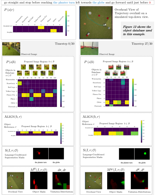
Figure 5 illustrates how the model reasoning when following an instruction can be visualized.

Appendix B Model Details

Figure 6 shows a whole-page version of Figure 3 from the main paper.

Figure 6: Full-page version of Figure 3. Policy architecture illustration. The first stage uses our few-shot language-conditioned segmentation to identify mentioned objects in the image. The segmentation and instruction embedding are used to generate an allocentric object context grounding map $\mathbf{C}^{W}_{t}$, a learned map of the environment that encodes at every position the behavior to be performed at or near it. We use LingUNet to predict visitation distributions, which the second stage maps to velocity commands. The components in blue are adopted from prior work [26, 6], while we add the components in green to enable few-shot generalization.

B.1 Object Reference Classifier ObjRef

The object reference classifier ObjRef inputs are a sequence of tokens representing a noun chunk and the object database $\mathcal{O}$. The output is True if the noun chunk refers to a physical object, and False otherwise.

We represent noun chunks with pre-trained GloVe vectors [37]. We use the en_core_web_lg model from the SpaCy library [40]. The classifier considers a noun chunk an object reference if either (a) a neural network object reference classifier assigns it a high score, or (b) the noun chunk is substantively similar to a phrase in the object database $\mathcal{O}$. The classifier decision rule for a noun chunk $\hat{r}$ is:

$$\textsc{ObjRef}(\hat{r},\mathcal{O})=\textsc{ObjRefNN}(\textsc{GloVe}(\hat{r}))+\lambda_{R1}\min_{o^{(i)}\in\mathcal{O}}\min_{j}\|\textsc{GloVe}(\hat{r})-\textsc{GloVe}(Q_{j}^{(i)})\|_{2}^{2}<T_{R2}\;,$$ (6)

where ObjRefNN is a two-layer fully connected neural network, GloVe is a function that represents a phrase as the average of its token GloVe embeddings, $\lambda_{R1}$ is a hyperparameter that balances between the database-agnostic network ObjRefNN and similarity to the object database $\mathcal{O}$, and $T_{R2}$ is a hyperparameter that adjusts precision and recall.

The classifier is trained on a dataset $\mathcal{D}_{R}=\{(\hat{r}^{(k)},l^{(k)})\}_{k}$ of noun chunks paired with labels $l^{(k)}\in\{0,1\}$ indicating whether the noun chunk is an object reference. The procedure for extracting this data from a navigation instruction dataset is described in Appendix D.

B.2 Contextualized Object Representations

Figure 7 illustrates the neural network architecture of $\psi$ and the anonymized instruction representation $\mathbf{\hat{h}}$, where all objects mentions are replaced with placeholder tokens.

Figure 7: Context embedding illustration. On top is a (shortened) instruction $u$. The second row shows the corresponding anonymized instruction $\hat{u}$. In the third row, we represent each word in $\hat{u}$ with a vector from a look-up table (LUT), and then encode the sequence with a bi-directional LSTM. The hidden states at positions corresponding to object reference tokens are object reference context embeddings. The sum of all hidden states is the anonymized instruction representation.

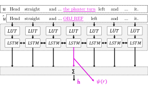
B.2.1 LingUNet Computation for Predicting Visitation Distributions

Figure 8: The LingUNet architecture. LingUNet outputs raw scores, which we normalize over the domain of each distribution. This figure is adapted from Blukis et al. [6].

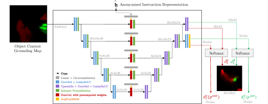
This section is adapted from Blukis et al. [6] and is included here for documentation completeness. Figure 8 illustrates the LingUNet architecture.

LingUNet uses a series of convolution and scaling operations. The input object context map $\mathbf{C}^{W}_{t}$ at time $t$ is processed through $L$ cascaded convolutional layers to generate a sequence of feature maps $\mathbf{F}_{k}=\textsc{CNN}^{D}_{k}(\mathbf{F}_{k-1})$, $k=1\dots L$. Each $\mathbf{F}_{k}$ is filtered with a 1$\times$1 convolution with weights $\mathbf{K}_{k}$. The kernels $\mathbf{K}_{k}$ are computed from the object-independent instruction representation $\mathbf{\hat{h}}$ using a learned linear transformation $\mathbf{K}_{k}=\mathbf{W}^{u}_{k}\mathbf{\hat{h}}+\mathbf{b}^{u}_{k}$. This generates $l$ language-conditioned feature maps $\mathbf{G}_{k}=\mathbf{F}_{k}\circledast\mathbf{K}_{k}$, $k=1\dots L$. A series of $L$ upscale and convolution operations computes $L$ feature maps of increasing size:

$$\mathbf{H}_{k}=\left\{\begin{array}[]{lr}{\textsc{Upscale}(\textsc{CNN}^{U}_{k}([\mathbf{H}_{k+1},\mathbf{G}_{k}]))},&\text{if }1\leq k\leq L-1\\ {\textsc{Upscale}(\textsc{CNN}^{U}_{k}(\mathbf{G}_{k}))},&\text{if }k=L\end{array}\right.\;\;.$$

An additional output head is used to output a vector h:

$$\textbf{h}=\textsc{AvgPool}(\textsc{CNN}^{\textbf{h}}(\mathbf{H}_{2}))\;\;,$$

where AvgPool takes the average across the spatial dimensions. h is the logit score assigned to the dummy location $p^{\texttt{oob}}$ representing all unobserved environment positions.

The output of LingUNet is a tuple ($\mathbf{H}_{1}$, h), where $\mathbf{H}_{1}$ is of size $W_{w}\times H_{w}\times 2$ and h is a vector of length 2. We apply a softmax operation across the spatial dimensions to produce the position visitation and goal visitation distributions given ($\mathbf{H}_{1}$, h).

B.3 Visitation Distribution Image Encoding

The visitation distributions $d^{p}_{t}$ and $d^{g}_{t}$ are represented by a four-channel square-shaped tensor of two spatial dimensions over the environment locations. Two channels correspond to the spatial domain of $d^{p}_{t}$ and $d^{g}_{t}$, and the other two channels are filled with uniform values $d^{p}_{t}(p^{\texttt{oob}})$ and $d^{g}_{t}(p^{\texttt{oob}})$. This four-channel encoding differs from the representation of Blukis et al. [6].

B.4 Control Network Architecture

The second policy stage $g(\cdot)$ generates the output velocities. It is implemented by a control network that receives from the first stage the visitation distribution encoding (Section B.3), an observability mask $\mathbf{M}^{W}_{t}$, and a boundary mask $\mathbf{B}^{W}_{t}$. The observability mask identifies locations in the environment that have been seen by the agent so far. The boundary mask indicates the four environment boundaries.

Figure 9: Control network architecture.

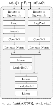
Figure 9 shows the control network architecture based on Blukis et al. [6]. We use two distinct copies of the control network, one as the policy Stage 2 action generator, and one as the value function for reinforcement learning as part of the SuReAL algorithm.

The visitation distributions $d^{p}_{t}$ and $d^{g}_{t}$ are represented by an image as described in Section B.3. This image is rotated to an egocentric reference frame defined by the agent’s current pose $P_{t}$, cropped to the agent’s immediate area, and processed with a convolutional neural network (CNN). The observability mask $\mathbf{M}^{W}_{t}$ and boundary mask $\mathbf{B}^{W}_{t}$ are concatenated along the channel dimension, spatially resized to the same pixel dimensions as the cropped visitation distributions, and processed with a convolutional neural network (CNN). The resulting representations of visitation distributions and masks are flattened, concatenated and processed with a densely-connected multi-layer perceptron.

The output of the action generation network consists of five scalars: The predicted forward and angular velocities $v$ and $\omega$, the logit of the stopping probability, and two standard deviations used during PPO training to define a continuous Gaussian probability distribution over actions.

Appendix C Learning Details

We train our model with SuReAL [6]. We remove the domain-adversarial discriminator. The algorithm’s two concurrent processes are described in Algorithms 1 and 2. The pseudocode is adapted from Blukis et al. [6] for documentation completeness.

Process A: Supervised Learning

Algorithm 1 shows the supervised learning process that is used to estimate the parameters $\theta$ of the first policy stage $f$. At every iteration, we sample executions from the dataset $\mathcal{D}^{\texttt{S}}$ (line 8) and update using the ADAM [45] optimizer (line 10) by optimizing the KL-divergence loss function:

$$\mathcal{L}_{\rm SL}(\Xi)=\frac{1}{|\Xi|}\sum_{c\in\mathcal{C}(\Xi)}D_{\rm KL}(f(c)\|f^{*}(c))$$ (8)

where $\mathcal{C}(\Xi)$ is the sequence of agent contexts observed during an execution $\Xi$, $f^{*}(c)$ creates the gold-standard visitation distributions (i.e., Stage 1 outputs) for a context $c$ from the training data, and $D_{\rm KL}$ is the KL-divergence operator. Every $K^{\rm SL}_{\rm iter}$ iterations, we send the policy stage 1 parameters to Process B (lines 12).

Process B: Reinforcement Learning

Algorithm 2 shows the reinforcement learning process that is used to estimate the parameters $\phi$ for the second policy stage $g$. This procedure is identical to the one described in Blukis et al. [6] and uses Proximal Policy Optimization [PPO; 46] to optimize an intrinsic reward function. At every iteration, we collect $N$ executions by rolling out the full policy $g(f_{\texttt{S}}(\cdot))$ in the simulator (line 8). We then perform $K^{\rm RL}_{\rm steps}$ parameter updates optimizing the PPO clipped policy-gradient loss (lines 9-12). We add the collected trajectories to the dataset shared with Process A (line 14). This allows the first policy stage $f$ to adapt its predicted distributions to the state-visitation distributions induced by the entire policy, making it robust to actions sampled from $g$. We find that this data sharing prevents $g$ from learning degenerative behaviors that exploit $f$.

We use the same intrinsic reward function as Blukis et al. [6]:

$$r(c_{t},a_{t})=\lambda_{v}r_{v}(c_{t},a_{t})+\lambda_{s}r_{s}(c_{t},a_{t})+\lambda_{e}r_{e}(c_{t},a_{t})-\lambda_{a}r_{a}(a_{t})-\lambda_{\rm step}\;\;,$$ (9)

where all $\lambda_{(\cdot)}$’s are constant hyperparameter weights, $r_{v}$ rewards correctly following the predicted trajectory distribution, $r_{s}$ rewards stopping at or near a likely stopping position according to the stopping distribution, $r_{e}$ rewards exploring the environment, and $r_{a}$ penalizes actions outside of controller range. See Blukis et al. [6] the formal definition of these terms.

Algorithm 1 Process A: Supervised Learning

1:First stage model $f$ with parameters $\theta$, dataset of simulated demonstration trajectories ${\mathcal{D}^{\texttt{S}}}$.

2:$f^{B}$ are shared with Process B.

3:$j\leftarrow 0$

4:repeat

5:   $j\leftarrow j+1$

6:   for $i=1,\dots,K^{\rm SL}_{\rm iter}$ do

7:      » Sample trajectory

8:      $\Xi^{\texttt{S}}\sim\mathcal{D}^{\texttt{S}}$

9:      » Update first stage parameters

10:      $\theta\leftarrow\textsc{ADAM}(\nabla_{\theta}\mathcal{L}_{\rm SL}(\Xi))$    

11:   » Send $f_{\texttt{S}}$ to Process B if it is running

12:   $f_{\texttt{S}}^{B}\leftarrow f_{\texttt{S}}$

13:   if $j=K_{\rm iter}^{B}$ then

14:      Launch Process B (Algorithm 2)    

15:until Process B is finished

16:return $f$

Algorithm 2 Process B: Reinforcement Learning

1:Simulation dataset ${\mathcal{D}^{\texttt{S}}}$, second-stage model $g$ with parameters $\phi$, value function $V$ with parameters $\upsilon$, first-stage simulation model $f_{\texttt{S}}$.

2:$\textsc{Merge}(\mathcal{D},E)$ is a set of sentence-execution pairs including all instructions from $\mathcal{D}$, where each instruction is paired with an execution from $E$, or $\mathcal{D}$ if not in $E$. $\mathcal{D}^{\texttt{S}}$ and $f_{\texttt{S}}^{B}$ are shared with Process A.

3:for $e=1,\dots,K^{\rm RL}_{\rm epoch}$ do

4:   » Get the most recent update from Process A

5:   $f_{\texttt{S}}\leftarrow f_{\texttt{S}}^{B}$

6:   for $i=1,\dots,K^{\rm RL}_{\rm iter}$ do

7:      » Sample simulator executions of $N$ instructions

8:      $\hat{\Xi}^{(1)},...,\hat{\Xi}^{(N)}\sim g(f_{\texttt{S}}(\cdot))$

9:      for $j=1,\dots,K^{\rm RL}_{\rm steps}$ do

10:         » Sample state-action-return tuples and update

11:         $X\sim\hat{\Xi}_{1},...,\hat{\Xi}_{N}$

12:         $\phi,\upsilon\leftarrow\textsc{ADAM}(\nabla_{\phi,\upsilon}\mathcal{L}_{PPO}(X,V))$       

13:      » Update executions to share with Process A

14:      $\mathcal{D}^{\texttt{S}}\leftarrow\textsc{Merge}(\mathcal{D}^{\texttt{S}},\{\hat{\Xi}_{1},\dots,\hat{\Xi}_{N}\})$    

15:return $g$

Appendix D Extracting Object References from a Navigation Corpus

We assume access to a dataset $\{(u^{(i)},\Xi^{(i)},\Lambda^{(i)})\}_{i}$ of natural language instructions $u^{(i)}$, each paired with a demonstration trajectory $\Xi^{(i)}$ and an environment layout $\Lambda^{(i)}$ that is a set of objects and their poses in the environment.

Given a natural language instruction $u$, let $\textsc{Ch}(u)$ denote the multi-set of noun chunks that appear in the instruction. This includes object references, such as the blue box, and spurious noun chunks, such as the left. Let $\textsc{Ob}(\Lambda,\Xi)$ denote the set of objects that appear in the layout $\Lambda$ in the proximity of the trajectory $\Xi$, which we define as within $1.41m$. We assume that the noun chunks $\textsc{Ch}(u)$ describe a subset of objects $\textsc{Ob}(\Lambda,\Xi)$ and use an alignment model similar to IBM Model 1 [47] to estimate the probabilities $p_{\gamma}(r\mid o)$ for a phrase $r\in\textsc{Ch}(u)$ and an object $o\in\textsc{Ob}(\Lambda,\Xi)$. The distribution is parameterized by $\gamma$, and is implemented with a one-layer long short-term memory network [LSTM; 41]. The input is a one-hot vector indicating the object type. The output is a sequence of tokens. The vocabulary is a union of all words in all training instructions. Noun chunks that do not refer to any landmark (e.g., left side, full stop, the front) are aligned with a special Null object.

Given a noun chunk $r$, we use the alignment model $p_{\gamma}(r\mid o)$ to infer the object $o$ referred by $r$:

$$o=\arg\max_{o\in\textsc{Ob}(\Lambda,\Xi)}p_{\gamma}(r\mid o)p(o)\;\;,$$ (10)

where $p(o)$ is estimated using object frequency counts in training data. We use this process to extract a dataset of over 4,000 textual object references, each paired with an object label. The language includes diverse ways of referring to the same object, such as the barrel, the lighter colored barrel, the silver barrel, white cylinder, and white drum. This technique is applicable to any vision and language navigation dataset that includes object annotations, such as the commonly used R2R dataset [12].

Appendix E Natural Language Navigation Data Details

We use the natural language instruction data from Misra et al. [13] and Blukis et al. [6] for training, and collect additional data with new objects. Table 2 shows basic statistics for all the data available to us. Table 3 summarizes how we used this data in our different experiments. The FsPVN and PVN2-SEEN models were trained on the ‘‘Train Seen’’ data split that includes data with 63 objects. The instructions used to train the policy include the 15 seen objects. This data excludes the eight unseen objects. The language-conditioned segmentation component is pre-trained on AR data, and is never tuned to adapt to the visual appearance of any of these objects. The PVN2-ALL model was trained on the ‘‘Train All’’ data split that includes 71 objects, including the 15 seen and eight unseen objects. The development results on eight new objects were obtained by evaluating on the ‘‘Dev Unseen’’ data split. The test results on 8 new objects were obtained by evaluating on the ‘‘Test Unseen’’ data split. The test results on 15 previously seen objects were obtained by evaluating on the ‘‘Test Seen’’ data split. We restrict the number of instructions in development and test datasets to a realistic scale for physical quadcopter experiments.

Dataset	Type	Split	# Paragraphs	# Instr.	Avg. Instr. Len.	Avg. Path
					(tokens)	Len. (m)
Lani	(A) 1-segment	(a) Train	4200	19762	11.04	1.53
		(b) Dev	898	4182	10.94	1.54
		(c) Test	902	4260	11.23	1.53
	(B) 2-segment	(a) Train	4200	15919	21.84	3.07
		(b) Dev	898	3366	21.65	3.10
		(c) Test	902	3432	22.26	3.07
Real	(A) 1-segment	(a) Train	698	3245	11.10	1.00
		(b) Dev	150	640	11.47	1.06
		(c) Test	149	672	11.31	1.06
	(B) 2-segment	(a) Train	698	2582	20.97	1.91
		(b) Dev	150	501	21.42	2.01
		(c) Test	149	531	21.28	1.99
Unseen	(A) 1-segment	(a) Train	692	2790	13.60	1.20
		(b) Dev	147	622	13.41	1.16
		(c) Test	147	577	13.14	1.25
	(B) 2-segment	(a) Train	692	2106	25.39	2.28
		(b) Dev	147	476	24.87	2.17
		(c) Test	147	431	24.77	2.39

Table 2: Dataset and split sizes. Lani was introduced by Misra et al. [13] and contains a total of 63 different objects in simulation only. Real is additional data introduced by Blukis et al. [6] with 15 objects that are a subset of Lani objects for use on the physical drone or simulation. Unseen is data that we collected containing environments with only 8 new objects that did not appear in Lani or Real data. It allows us to train models on data from Lani and Real, while testing on data with previously unseen objects from Unseen. The 2-segment data consists of instructions made of two 1-segment consecutive instructions concatenated together.

Data Split	# Instr.	Source from data splits in Table 2.
Train Seen	41508	Lani.A.a $\cup$ Lani.B.a $\cup$ Real.A.a $\cup$ Real.B.a
Train All	46404	Lani.A.a $\cup$ Lani.B.a $\cup$ Real.A.a $\cup$ Real.B.a $\cup$ Unseen.A.a $\cup$ Unseen.B.a
Dev Unseen	103	Random subset of Unseen.B.b
Test Unseen	63	Random subset of Unseen.B.c
Test Seen	73	Random subset of Real.B.c

Table 3: Dataset splits used for training, development and testing in our experiments in Section 8, showing the number of instructions, and how each data split was obtained from the available data summarized in Table 2

E.1 List of Seen and Unseen Objects

Figure 10: The list of seen (top) and unseen (bottom) objects during training in both the physical and real-world environments.

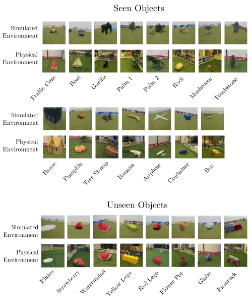
Figure 10 shows the set of seen and unseen objects in the simulated and physical environments. An additional 48 simulation-only objects that are seen during training are not shown. The agent does not see the unseen objects or references to them during training.

Appendix F Augmented Reality Object Image Data

Figure 11: Examples from the augmented reality object data in the physical (top) and simulated (bottom) environments.

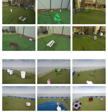
The training procedure for the few-shot language-conditioned segmentation component uses a dataset $\mathcal{D}_{o}=\{(I^{(i)},\{(b^{(i)}_{j},m^{(i)}_{j},o^{(i)}_{j})\}_{j})\}_{i}$ (Section 4.2). This data includes a large number of diverse objects that cover general object appearance properties, such as shape, colors, textures, and size, to allow generalizing to new objects. Collecting such data in a real-world environment is costly. Instead, we generate 20,000 environment layouts that consist of 6--16 objects drawn from a pool of 7,441 3D models from ShapeNet [44]. We use only objects where the longest edge of the axis-aligned bounding box is less than five times grater than the shorter edge. This excludes planar objects such as paintings. We use augmented reality to instantiate the objects in the physical and simulated environments. We collect a set of images of empty environments with no objects by flying the quadcopter along randomly generated trajectories. We use the Panda3D [48] rendering engine to render objects over the observed images, as if they are physically present in the environment. Figure 11 shows example observations. This process also automatically generates bounding box annotations tagged with object identities. The diverse shapes and textures of objects allow us to learn a view-point invariant object similarity metric, however it creates the challenge of generalizing from relatively simple ShapeNet objects to physical objects. It is possible to load the ShapeNet objects within the simulator itself, but we opted to use the AR approach in both simulated and physical environments to ensure uniform data format.

Appendix G Object Databases

Figure 12: The object database used during testing, containing previously unseen physical objects.

Figure 13: The object database used during testing, containing previously unseen simulated objects.

Figure 14: The object database used during development in the physical environment.

Figure 15: The object database used during development in the simulation..

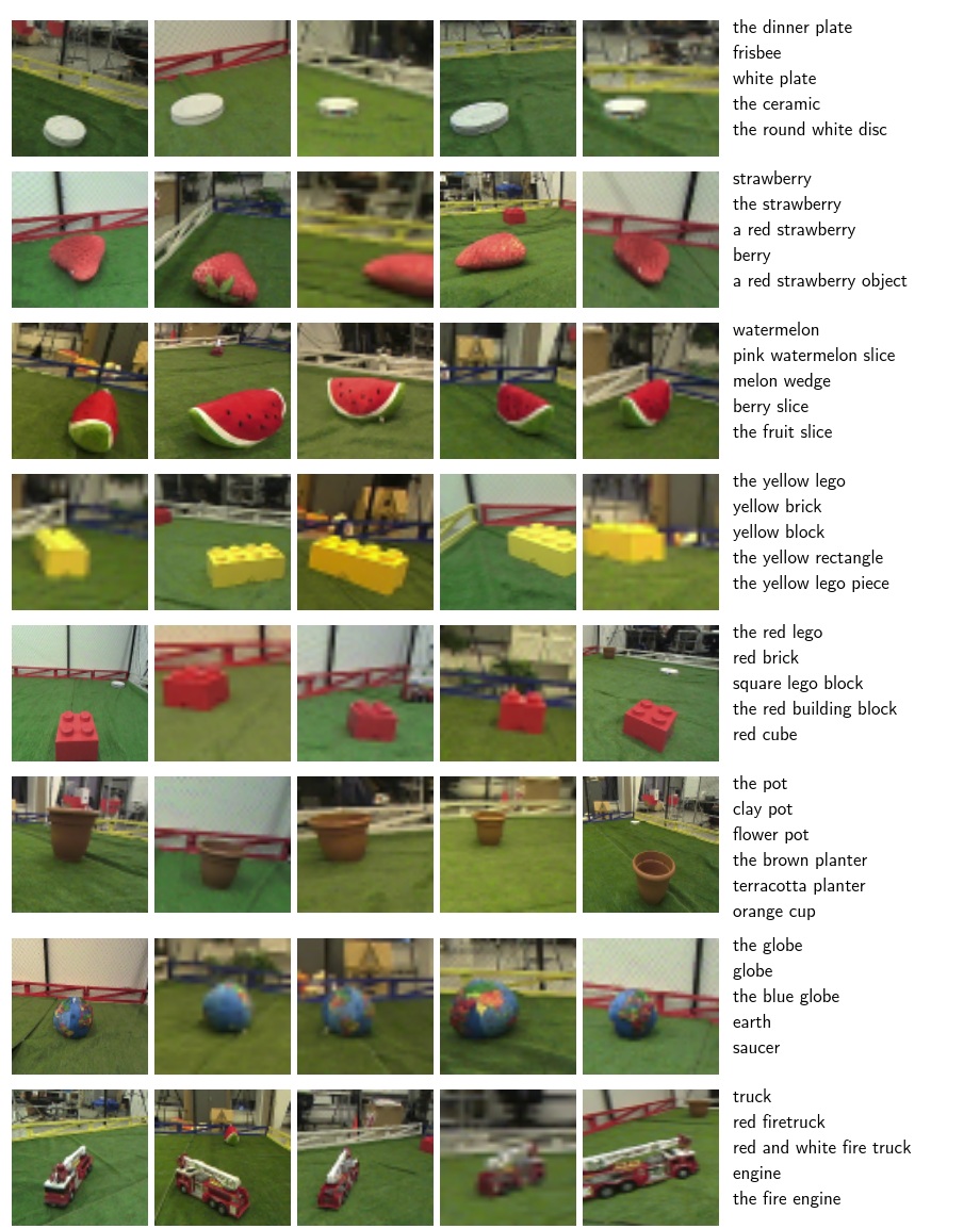
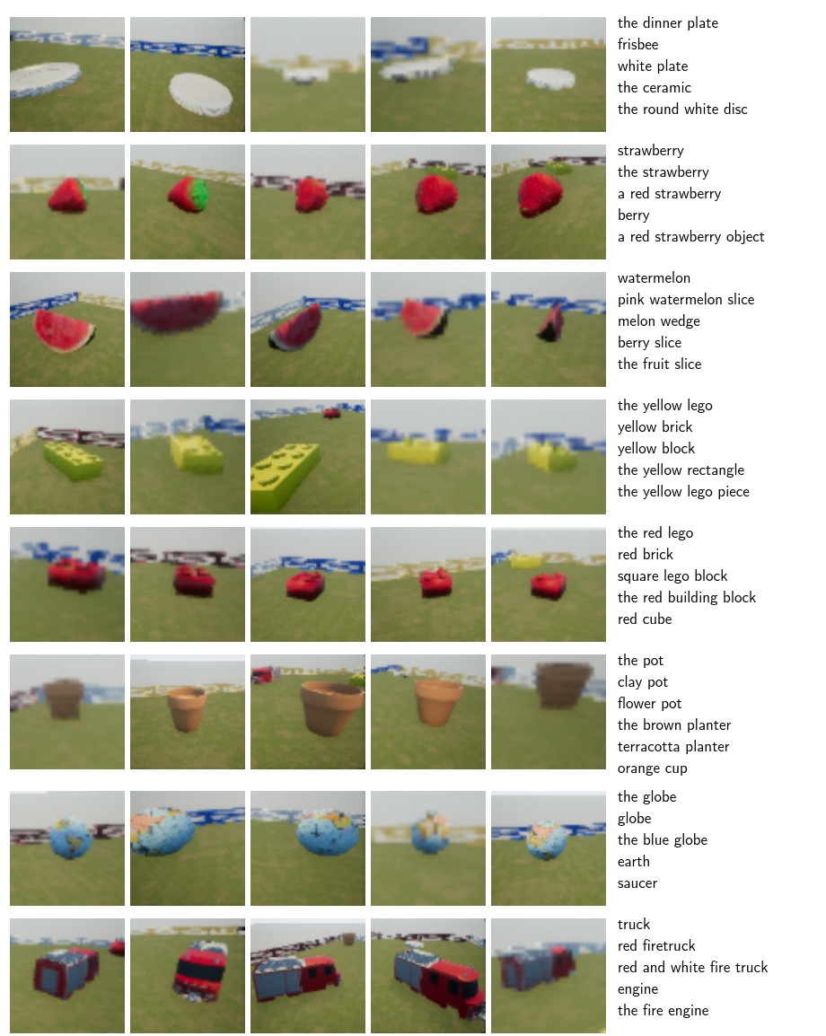
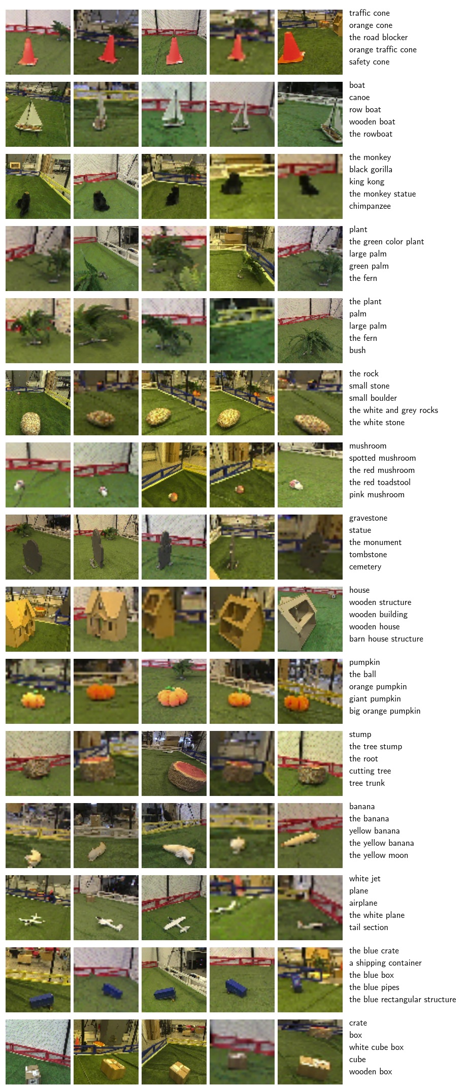
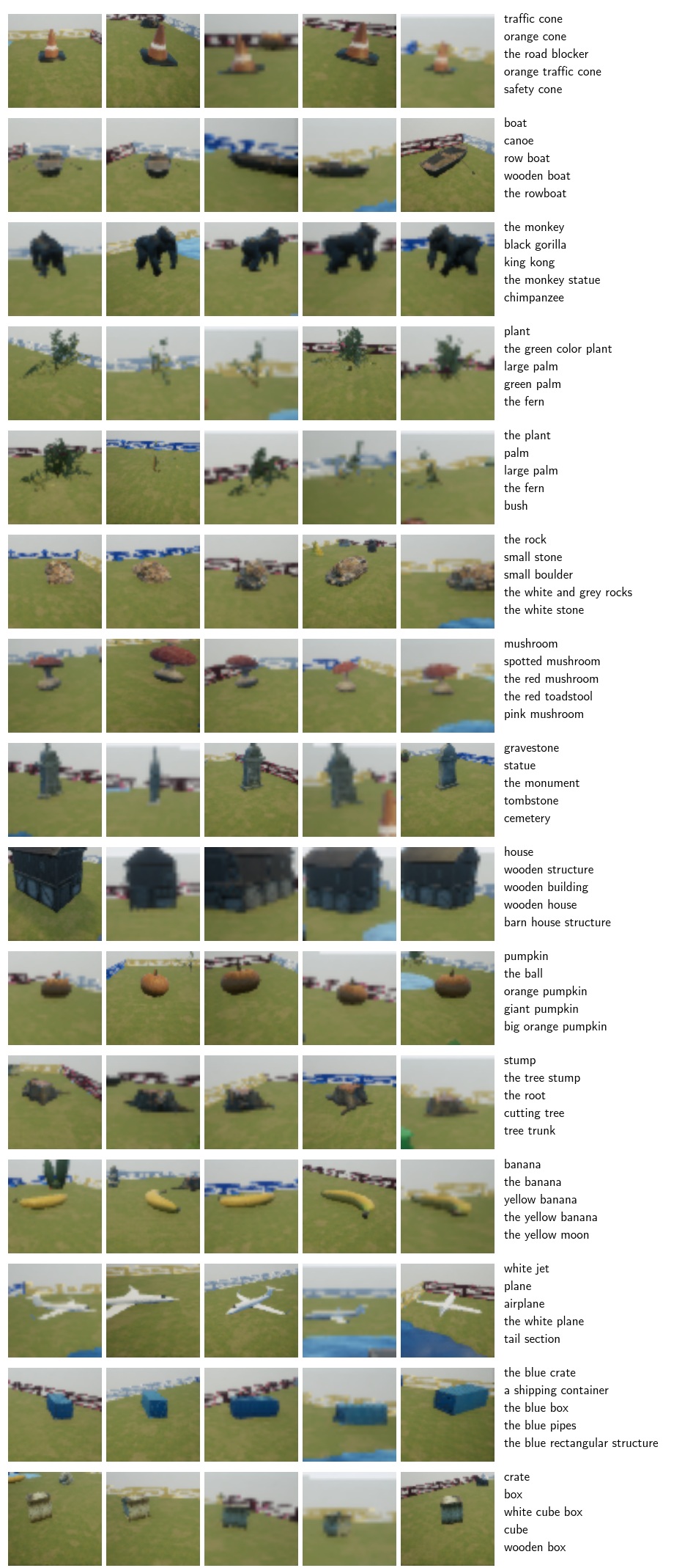
The object database $\mathcal{O}$ consists of a set of objects, each represented by five images and five textual descriptions. We use different object databases during training, development evaluation on seen objects, and test-time evaluation on unseen object. For each database, the images and textual descriptions are taken from a pre-collected pool. Object images are obtained by collecting a set of trajectories from the $\pi^{*}$ policy in random training environments, cropping out a region around each object in the image, and storing each image tagged by the object type. The textual description are obtained by first extracting all noun chunks in every instruction of the Lani dataset training split using SpaCy [40], and using Equation 10 to match each noun chunk to the object it refers to.

G.1 Object Database Figures

Test-time Database for Evaluation with Unseen Objects

Figure 12 shows the object database used at test-time on the physical quadcopter containing unseen objects only. The agent has not seen these objects before, and the only information it has available about these objects is the database. The images and textual descriptions are hand-selected from the pre-collected pool to be diverse and representative. Figure 13 shows the same content for the simulation.

Development Database for Evaluation with Seen Objects

Figure 14 shows the object database used for evaluation during development on the physical quadcopter containing objects that the agent has seen during training. The images and textual descriptions are hand-selected from the pre-collected pool to be diverse and representative. Figure 15 depicts the same content for the simulation.

Generation of Object Databases Used During Training

Each training example is a tuple $(u,\Xi)$ situated in an environment layout $\Lambda$ that specifies the set of objects in the environment and their poses. We generate an object database $\mathcal{O}$ for each training example by creating an entry in the database for each object $o\in\Lambda$. We pair each object with five images randomly selected from the pre-collected image pool, and five object references randomly selected from the pre-collected textual description pool.

Appendix H Additional Evaluation

Language-Conditioned Segmentation Evaluation

Automatic evaluation of our language-conditioned segmentation is not possible due to a lack of ground-truth alignments between object references in the instructions and object masks. We manually evaluate our language-conditioned segmentation method on 40 policy rollouts from the development data containing unseen objects to assess its performance in isolation. For each rollout, we subjectively score the segmentation mask output with a score of 1--3, where 1 means the output is wrong or missing, 2 means that at least one of the mentioned objects has been identified, and 3 means that all mentioned objects have been correctly identified, allowing only for slight visual artifacts in mask boundaries. Because each rollout consists of a sequence of images, we allow for some images to contain false negatives, so long as the mentioned objects are eventually identified in a way that conceivably allows the policy to complete the task. Our approach achieved a 3-point score on 82.5% of the rollouts.

Image Similarity Measure Evaluation

We automatically evaluate the image similarity model ImgEmb in isolation on a 2-way, 8-way, and 15-way classification task using 2429 images of 15 physical objects in the drone environment. We use the set of ‘‘seen’’ objects (Figure 14). In each evaluation example, we randomly sample a query object with five random query images, and a set of target objects with five random images each. The set of target objects includes the query object, but with a different set of images. We test the ability of the image similarity model ImgEmb to classify which of the target objects has the same identity as the query object.

We find that in the 2-way classification task (n=11480), the image similarity model achieves 92% accuracy in identifying the correct target object. In a 8-way classification task (n=14848) the accuracy drops to 73%, and on a 15-way classification task (n=14848), it drops to 63%. The model has never observed these objects, and generalizes to them from AR training data only.

The language-conditioned few-shot segmentation model combines both visual and language modalities to identify an object and produce an instance segmentation mask, considering every object in the database. This is why the segmentation model that uses ImgEmb can achieve a higher segmentation performance than ImgEmb achieves on a classification task in isolation.

Appendix I Implementation Details

I.1 Hyperparameter Settings

Table 4 shows the hyperparameter assignments. We started with the initial values from  Blukis et al. [6], and tuned the parameters relating to our few-shot grounding approach.

Hyperparameter	Value
Environment Settings
Maximum yaw rate	$\omega_{\rm max}=1m/s$
Maximum forward velocity	$v_{\rm max}=0.7m/s$
Image and Feature Dimensions
Camera horizontal FOV	$84^{\circ}$
Input image dimensions	$128\times 72\times 3$
Object mask $\mathbf{M}^{W}$ dimensions	$32\times 32\times 1$
Object context map $\mathbf{C}^{W}$ dimensions	$32\times 32\times 40$
Visitation distributions $d^{g}$ and $d^{p}$ dimensions	$64\times 64\times 1$
Database object image $Q$ dimensions	$32\times 32\times 3$
Environment edge length in meters	$4.7m$
Few-shot Language-Conditioned Segmentation
Image metric learning margin	$T_{M1}=1.0$
Image metric learning margin	$T_{M2}=2.0$
Image kernel density estimation std. dev.	$\sigma=2.0$
Text kernel density estimation std. dev.	$\sigma=0.5$
Object reference recognizer weight	$\lambda_{R1}=0.5$
Object reference recognizer threshold	$\lambda_{R2}=0.03$
General Learning
Deep Learning library	PyTorch 1.4.1
Supervised Learning
Optimizer	ADAM
Learning Rate	$0.001$
Weight Decay	$10^{-6}$
Batch Size	$1$
Reinforcement Learning (PPO)
Num supervised epochs before starting RL ($K_{iter}^{B}$)	30
Num epochs ($K_{\rm epoch}^{\rm RL}$)	200
Iterations per epoch ($K_{\rm iter}^{\rm RL})$	50
Number of parallel actors	4
Number of rollouts per iteration $N$	20
PPO clipping parameter	0.1
PPO gradient updates per iter ($K_{\rm steps}^{\rm RL})$	8
Minibatch size	2
Value loss weight	1.0
Learning rate	0.00025
Epsilon	1e-5
Max gradient norm	1.0
Use generalized advantage estimation	False
Discount factor ($\gamma$)	0.99
Entropy coefficient	0.001
Reward Weights
Stop reward weight ($\lambda_{s}$)	0.5
Visitation reward weight($\lambda_{v}$)	0.3
Exploration reward weight ($\lambda_{e}$)	1.0
Negative per-step reward ($\lambda_{\rm step}$)	-0.04

Table 4: Hyperparameter values.

References

- Tellex et al. [2011] S. Tellex, T. Kollar, S. Dickerson, M. R. Walter, A. Gopal Banerjee, S. Teller, and N. Roy. Approaching the Symbol Grounding Problem with Probabilistic Graphical Models. AI Magazine, 2011.
- Duvallet et al. [2013] F. Duvallet, T. Kollar, and A. Stentz. Imitation learning for natural language direction following through unknown environments. In ICRA, 2013.
- Misra et al. [2014] D. K. Misra, J. Sung, K. Lee, and A. Saxena. Tell me dave: Context-sensitive grounding of natural language to mobile manipulation instructions. In RSS, 2014.
- Hemachandra et al. [2015] S. Hemachandra, F. Duvallet, T. M. Howard, N. Roy, A. Stentz, and M. R. Walter. Learning models for following natural language directions in unknown environments. In ICRA, 2015.
- Gopalan et al. [2018] N. Gopalan, D. Arumugam, L. L. Wong, and S. Tellex. Sequence-to-sequence language grounding of non-markovian task specifications. In RSS, 2018.
- Blukis et al. [2019] V. Blukis, Y. Terme, E. Niklasson, R. A. Knepper, and Y. Artzi. Learning to map natural language instructions to physical quadcopter control using simulated flight. In CoRL, 2019.
- Matuszek et al. [2012] C. Matuszek, N. FitzGerald, L. Zettlemoyer, L. Bo, and D. Fox. A Joint Model of Language and Perception for Grounded Attribute Learning. In ICML, 2012.
- Thomason et al. [2015] J. Thomason, S. Zhang, R. J. Mooney, and P. Stone. Learning to interpret natural language commands through human-robot dialog. In IJCAI, 2015.
- Williams et al. [2018] E. C. Williams, N. Gopalan, M. Rhee, and S. Tellex. Learning to parse natural language to grounded reward functions with weak supervision. In ICRA, 2018.
- Misra et al. [2017] D. Misra, J. Langford, and Y. Artzi. Mapping instructions and visual observations to actions with reinforcement learning. In EMNLP, 2017.
- Shah et al. [2018] P. Shah, M. Fiser, A. Faust, J. C. Kew, and D. Hakkani-Tur. Follownet: Robot navigation by following natural language directions with deep reinforcement learning. arXiv preprint arXiv:1805.06150, 2018.
- Anderson et al. [2018] P. Anderson, Q. Wu, D. Teney, J. Bruce, M. Johnson, N. Sünderhauf, I. Reid, S. Gould, and A. van den Hengel. Vision-and-language navigation: Interpreting visually-grounded navigation instructions in real environments. In CVPR, 2018.
- Misra et al. [2018] D. Misra, A. Bennett, V. Blukis, E. Niklasson, M. Shatkin, and Y. Artzi. Mapping instructions to actions in 3D environments with visual goal prediction. In EMNLP, 2018.
- Fried et al. [2018] D. Fried, R. Hu, V. Cirik, A. Rohrbach, J. Andreas, L.-P. Morency, T. Berg-Kirkpatrick, K. Saenko, D. Klein, and T. Darrell. Speaker-follower models for vision-and-language navigation. In NeurIPS, 2018.
- Jain et al. [2019] V. Jain, G. Magalhaes, A. Ku, A. Vaswani, E. Ie, and J. Baldridge. Stay on the path: Instruction fidelity in vision-and-language navigation. In ACL, 2019.
- Blukis et al. [2018] V. Blukis, D. Misra, R. A. Knepper, and Y. Artzi. Mapping navigation instructions to continuous control actions with position-visitation prediction. In CoRL, 2018.
- Paxton et al. [2019] C. Paxton, Y. Bisk, J. Thomason, A. Byravan, and D. Foxl. Prospection: Interpretable plans from language by predicting the future. In ICRA, pages 6942--6948. IEEE, 2019.
- Roh et al. [2020] J. Roh, C. Paxton, A. Pronobis, A. Farhadi, and D. Fox. Conditional driving from natural language instructions. In CoRL, pages 540--551, 2020.
- Shridhar et al. [2020] M. Shridhar, J. Thomason, D. Gordon, Y. Bisk, W. Han, R. Mottaghi, L. Zettlemoyer, and D. Fox. Alfred: A benchmark for interpreting grounded instructions for everyday tasks. In CVPR, June 2020.
- Lenz et al. [2015] I. Lenz, H. Lee, and A. Saxena. Deep learning for detecting robotic grasps. IJRR, 2015.
- Levine et al. [2016] S. Levine, P. Pastor, A. Krizhevsky, and D. Quillen. Learning hand-eye coordination for robotic grasping with large-scale data collection. In ISER, 2016.
- Quillen et al. [2018] D. Quillen, E. Jang, O. Nachum, C. Finn, J. Ibarz, and S. Levine. Deep reinforcement learning for vision-based robotic grasping: A simulated comparative evaluation of off-policy methods. ICRA, 2018.
- Nair et al. [2017] A. Nair, D. Chen, P. Agrawal, P. Isola, P. Abbeel, J. Malik, and S. Levine. Combining self-supervised learning and imitation for vision-based rope manipulation. In ICRA, 2017.
- Tan et al. [2019] H. Tan, L. Yu, and M. Bansal. Learning to navigate unseen environments: Back translation with environmental dropout. In NAACL-HLT, 2019.
- Gordon et al. [2018] D. Gordon, A. Kembhavi, M. Rastegari, J. Redmon, D. Fox, and A. Farhadi. Iqa: Visual question answering in interactive environments. In CVPR, 2018.
- Blukis et al. [2018] V. Blukis, N. Brukhim, A. Bennet, R. Knepper, and Y. Artzi. Following high-level navigation instructions on a simulated quadcopter with imitation learning. In RSS, 2018.
- Snell et al. [2017] J. Snell, K. Swersky, and R. Zemel. Prototypical networks for few-shot learning. In NIPS, pages 4077--4087, 2017.
- Wertheimer and Hariharan [2019] D. Wertheimer and B. Hariharan. Few-shot learning with localization in realistic settings. In CVPR, June 2019.
- Wang et al. [2017] Y.-X. Wang, D. Ramanan, and M. Hebert. Learning to model the tail. In NIPS, pages 7029--7039, 2017.
- Gao et al. [2019] N. Gao, Y. Shan, Y. Wang, X. Zhao, Y. Yu, M. Yang, and K. Huang. Ssap: Single-shot instance segmentation with affinity pyramid. In ICCV, 2019.
- Roy et al. [2019] S. Roy, M. Noseworthy, R. Paul, D. Park, and N. Roy. Leveraging past references for robust language grounding. In CoNLL, 2019.
- Margffoy-Tuay et al. [2018] E. Margffoy-Tuay, J. C. Pérez, E. Botero, and P. Arbeláez. Dynamic multimodal instance segmentation guided by natural language queries. In ECCV, 2018.
- Yu et al. [2018] L. Yu, Z. Lin, X. Shen, J. Yang, X. Lu, M. Bansal, and T. L. Berg. Mattnet: Modular attention network for referring expression comprehension. In CVPR, pages 1307--1315, 2018.
- Cirik et al. [2018] V. Cirik, L.-P. Morency, and T. Berg-Kirkpatrick. Visual referring expression recognition: What do systems actually learn? In NAACL-HLT, pages 781--787, 2018.
- Shridhar and Hsu [2018] M. Shridhar and D. Hsu. Interactive visual grounding of referring expressions for human-robot interaction. In RSS, 2018.
- Wu et al. [2019] Y. Wu, A. Kirillov, F. Massa, W.-Y. Lo, and R. Girshick. Detectron2. https://github.com/facebookresearch/detectron2, 2019.
- Pennington et al. [2014] J. Pennington, R. Socher, and C. D. Manning. Glove: Global vectors for word representation. In EMNLP, 2014.
- Ronneberger et al. [2015] O. Ronneberger, P. Fischer, and T. Brox. U-net: Convolutional networks for biomedical image segmentation. In International Conference on Medical image computing and computer-assisted intervention, 2015.
- Tjong Kim Sang and Buchholz [2000] E. F. Tjong Kim Sang and S. Buchholz. Introduction to the CoNLL-2000 shared task chunking. In CoNLL, 2000.
- Honnibal and Montani [2017] M. Honnibal and I. Montani. spaCy 2: Natural language understanding with Bloom embeddings, convolutional neural networks and incremental parsing. To appear, 2017.
- Hochreiter and Schmidhuber [1997] S. Hochreiter and J. Schmidhuber. Long short-term memory. Neural computation, 1997.
- Anderson et al. [2019] P. Anderson, A. Shrivastava, D. Parikh, D. Batra, and S. Lee. Chasing ghosts: Instruction following as bayesian state tracking. In NeurIPS, 2019.
- Krantz et al. [2020] J. Krantz, E. Wijmans, A. Majumdar, D. Batra, and S. Lee. Beyond the nav-graph: Vision-and-language navigation in continuous environments. arXiv preprint arXiv:2004.02857, 2020.
- Chang et al. [2015] A. Chang, T. Funkhouser, L. Guibas, P. Hanrahan, Q. Huang, Z. Li, S. Savarese, M. Savva, S. Song, H. Su, J. Xiao, L. Yi, and F. Yu. Shapenet: An information-rich 3d model repository. 2015.
- Kingma and Ba [2015] D. P. Kingma and J. Ba. Adam: A method for stochastic optimization. ICLR, 2015.
- Schulman et al. [2017] J. Schulman, F. Wolski, P. Dhariwal, A. Radford, and O. Klimov. Proximal policy optimization algorithms. arXiv preprint arXiv:1707.06347, 2017.
- Brown et al. [1993] P. F. Brown, V. J. D. Pietra, S. A. D. Pietra, and R. L. Mercer. The mathematics of statistical machine translation: Parameter estimation. Computational linguistics, 19(2):263--311, 1993.
- Goslin and Mine [2004] M. Goslin and M. R. Mine. The panda3d graphics engine. Computer, 2004.