A unified and automated approach to attractor reconstruction

Abstract

We present a fully automated method for the optimal state space reconstruction from univariate and multivariate time series. The proposed methodology generalizes the time delay embedding procedure by unifying two promising ideas in a symbiotic fashion. Using non-uniform delays allows the successful reconstruction of systems inheriting different time scales. In contrast to the established methods, the minimization of an appropriate cost function determines the embedding dimension without using a threshold parameter. Moreover, the method is capable of detecting stochastic time series and, thus, can handle noise contaminated input without adjusting parameters. The superiority of the proposed method is shown on some paradigmatic models and experimental data from chaotic chemical oscillators.

I Introduction

State space reconstruction from observational time series often marks the first and basic step in nonlinear time series analysis. Several methods addressed the reconstruction problem, but none of them allow for a fully automatized and reliable way of embedding a uni- or multivariate set of observed time series with no, or at least very few, free parameters. The aim of this paper is to provide such a technique. The embedding theorems of Whitney (1936), Mañé (1981), and Takens (1981) among with their extension by Sauer et al. (1991) allow several approaches to tackle the reconstruction problem. Among using derivative coordinates Broomhead and King (1986); Mann et al. (2011), PCA Packard et al. (1980) or Legendre coordinates Gibson et al. (1992), uniform- and nonuniform time delay embedding Packard et al. (1980) is by far the most commonly used technique, due to its appealing simplicity. However, since Takens’ theorem Takens (1981) is based on noise-free and infinitely long data, it does not give any guidance to choose the proper time delay(s) $\tau$ in practice. Together with the unknown box-counting dimension $D_{B}$ of the observed, but unknown system, which is needed to fulfil the embedding dimension criterion $m\geqslant 2D_{B}+1$, the majority of the published articles propose ideas to infer estimates for $\tau$ and the reconstruction dimension $m$ from data, usually a univariate time series (univariate embedding). The reconstruction problem starts with the unknown system $\vec{u}(t)$ with a mapping $f:\mathbb{R}^{D_{B}}\to\mathbb{R}^{D_{B}}$, which is observed via a measurement function $h$ and lead to $M$ observational time series $\{s_{i}(t)|i=1,\ldots,M\}$ (Fig. 1). There can be different measurement functions $h^{\prime}$ forming the multivariate dataset $s_{i}(t)$ and the combination of Whitney’s and Takens’ embedding theorems allow for constructing $\vec{u}(t)$ from more than one time series (multivariate embedding) Sauer et al. (1991); Deyle and Sugihara (2011). One then tries to find optimal embedding parameters $m$ and $\tau$’s (the delays can be integer multiple of some constant, uniform time delay embedding UTDE, or different for each embedding dimension, non-uniform time delay embedding NUTDE) in order to build reconstruction vectors $\vec{v}(t)$ and, thus, a mapping $F:\mathbb{R}^{m}\to\mathbb{R}^{m}$. These can be furthermore transformed by $\Psi$ into $\vec{v}^{\prime}(t)$ and $F^{\prime}$, preserving the diffeomorphism to $\vec{u}(t)$. For a detailed introduction into the reconstruction problem we refer to Casdagli et al. (1991), Gibson et al. (1992), Uzal et al. (2011) or Nichkawde (2013).

Figure 1: Schematic representation of the embedding/reconstruction procedure. See the text for details. This figure is inspired by Casdagli et al. (1991) and Uzal et al. (2011).

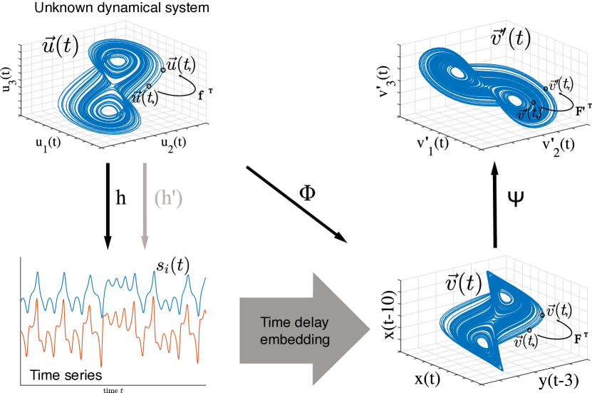
In time delay embedding the key idea is to use lagged values of the available time series as components of the reconstruction vector

$$\vec{v}(t)=\bigl{(}s_{i_{1}}(t-\tau_{1}),s_{i_{2}}(t-\tau_{2}),\ldots,s_{i_{m}}(t-\tau_{m})\bigl{)}.$$ (1)

The delays $\tau_{j}$ and the corresponding time series $s_{i_{j}},j=[1,\ldots,m]$ should be chosen, such that the resulting components of the vectors forming the reconstructed state space $\vec{v}(t)$ are as independent as possible (Packard et al., 1980; Sauer et al., 1991), but at the same time preserve the correlation structure of the system to a certain extent. These two competing objectives are also known as the problems of redundancy (delays should not be too small) and irrelevance (delays should not be too large) Casdagli et al. (1991); Rosenstein et al. (1994); Eftekhari et al. (2018); Uzal et al. (2011) and its optimization is goal to any proposed time delay embedding procedure.

Despite of its lack of a sound theoretical foundation for higher dimensional reconstructions ($m>2$) Grassberger et al. (1991); Vlachos and Kugiumtzis (2010); Fraser (1989), in a univariate scenario (i.e., $s_{i_{1}}=\ldots=s_{i_{m}}=s(t)$ in Eq. (1)), the approach to choose $\tau_{2}$ from the first minimum of the auto-mutual information Fraser and Swinney (1986); Liebert and Schuster (1989) is most common. $\tau_{1}$ is usually set to zero, i.e. the unlagged time series constitutes the first component of the reconstruction vectors. The embedding dimension $m$ is then separately determined, usually by a false nearest neighbour approach Kennel et al. (1992); Kennel and Abarbanel (2002); Cao (1997); Hegger and Kantz (1999); Tang et al. (2015) or some other neighbourhood-preserving-idea Aleksić (1991); Čenys and Pyragas (1988) and all delays up to $\tau_{m}$ are simply integer multiples of $\tau_{2}$ (UTDE). Other approaches for an appropriate choice of $\tau_{2}$ are possible Kember and Fowler (1993); Cao et al. (1998); Kugiumtzis (1996); Albano et al. (1988, 1991); Rosenstein et al. (1994); Aguirre (1995); Broomhead and King (1986). We refer to this as standard time delay embedding (TDE) in the following. More sophisticated ideas Liebert et al. (1991); Buzug et al. (1990); Buzug and Pfister (1992a, b); Kember and Fowler (1993); Gao and Zheng (1993, 1994); Judd and Mees (1998); Kim et al. (1999); Vlachos and Kugiumtzis (2010); Small and Tse (2004); Gao and Zheng (1994); Perinelli and Ricci (2018), some including non-uniform delays and the extension to multivariate input data Holstein and Kantz (2009); Nichkawde (2013); Garcia and Almeida (2005a, b); Pecora et al. (2007); Hirata et al. (2006); Han et al. (2019) have been presented Hirata and Aihara (2017); Han et al. (2019), but it seems their use is rather limited and not very popular. This could be due to their occasionally very complex nature and the lack of high quality open source implementation in the most commonly used programming languages. Another reason could be the fact that standard TDE performs surprisingly well in a range of examples; but still, its limitations should not be neglected, in particular when it comes to noisy time series, systems exhibiting multi-time scale behaviour, or multivariate input data. The latter are becoming of increasing interest in the near future, since acquisition costs for sensors and data collection decrease rapidly. Moreover, the application of complex systems approaches and nonlinear dynamics in different scientific disciplines receives increasing popularity.

Here we propose a fully automated method for an appropriate state space reconstruction of uni- or multivariate time series input, which utilizes two concepts, the continuity statistic Pecora et al. (2007) and the $L$-statistic Uzal et al. (2011). We briefly review the basic ideas we will use in our proposed method (Sect. II) in order to illustrate their specific utilization in the algorithm (Sect. III), before applying it to simulated and experimental data (Sect. IV).

II Review of used concepts

In order to ensure comprehensibility of our proposed method in Section III we explain the two main concepts of it in the following. In Section II.1 we review the continuity statistic Pecora et al. (2007) rather detailed, while the $L$-statistic is described only briefly in Section II.2 and extensively in the Appendix F.

II.1 Continuity statistic by Pecora et al.

In the continuity statistic, the problem of finding an optimal state space reconstruction with respect to redundancy and irrelevance is addressed by a statistical determination of functional independence among the components of the reconstruction vector Pecora et al. (2007). Let $\{s_{i}(t)|i=1,\ldots,M\}$ be a multivariate dataset consisting of $M$ time series, equally sampled at time instants $t=1,\ldots,N$. Suppose we have already chosen some delays $\tau_{k}$ to build our temporal reconstruction vector $\vec{v}(t)$ of dimension d. This is, $\vec{v}(t)=(s_{j_{1}}(t+\tau_{1}),s_{j_{2}}(t+\tau_{2}),\ldots,s_{j_{d}}(t+\tau_{d}))$, with $j_{k}\in\{1,\ldots,M\}$ being the choices of the different time series and $\tau_{k}$ the according delays, which can be – and most often are – different. Then for a new potential component of $\vec{v}(t)$ we ask if this new potential component can be expressed as a function of the existing components. Mathematically speaking, the equality

$$s_{j_{d+1}}(t+\tau_{d+1})\stackrel{{\scriptstyle?}}{{=}}f\left(s_{j_{1}}(t+\tau_{1}),s_{j_{2}}(t+\tau_{2}),\ldots,s_{j_{d}}(t+\tau_{d})\right)$$ (2)

needs to be tested in an appropriate way, i.e., a sensible choice for $f:\mathbb{R}^{d}\to\mathbb{R}^{1}$ has to be made. This choice can be based on the property of continuity Pecora et al. (1995).

Figure 2: Fiducial point (blue) and its $k=4$ nearest neighbours (green) in the d-dimensional $\delta$- ball (left panel). Arrows indicate the mapping $f:\mathbb{R}^{d}\to\mathbb{R}^{1}$ (right panel), which is the potential $(d+1)^{\text{th}}$ component of each of the points in the left panel (according to a specific delay $\tau_{d+1}$ and time series $s_{j_{d+1}}$), Eq. (2). To decide whether this $\varepsilon$-interval size accepts or rejects the null hypothesis on a significance level $\alpha$ the cumulative binomial distribution for getting at least $l=3$ points in the $\varepsilon$-interval with probability p is used (modified after Pecora et al. (2007)).

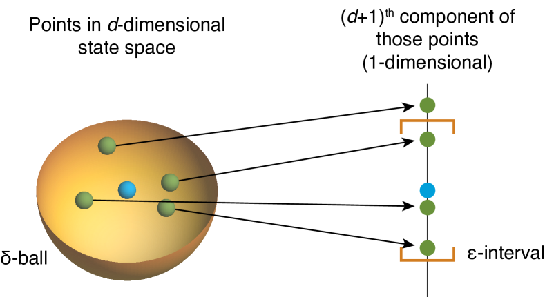
The practical implementation of Eq. (2) would start with mapping $k$ nearest neighbours, $\vec{v}_{k}(t)$, of a fiducial point $\vec{v}_{\text{fid}}(t)$ from $\mathbb{R}^{d}\to\mathbb{R}^{1}$, as illustrated in Fig. 2. That is, for each of the ($k+1$) d-dimensional points in the left panel a potential ($d+1$)th component $s_{j_{d+1}}(t+\tau_{d+1})$ is considered and drawn onto the number line (right panel). The continuity statistic now asks whether these $k+1$ points on the 1-dimensional number line fall within a certain $\varepsilon$-interval size by chance, or due to the fact that there is a functional relationship between the $d$ and the ($d+1$)th component of a potential reconstruction vector $\vec{v}(t)$. The according continuity null hypothesis is that $l$ of the $k+1$ points landed in the $\varepsilon$-interval by chance, with probability $p$ on the basis of the binomial distribution. When the number of observed neighbours, which are mapped into the $\varepsilon$-interval, is larger than the expected number from the binomial distribution for a selected $\alpha$, i.e. $l$ points, then the null can be rejected and, thus, a functional relationship can be assumed. The number of considered nearest neighbours $k$ (i.e., the size of the $\delta$-ball in Fig. 2) also determines the acceptable number of $k+1-l$ points falling outside the chosen $\varepsilon$-interval for a given probability parameter $p$ of the binomial distribution and a given $\alpha$. For each candidate delay $\tau_{d+1}$ and each time series $s_{j_{d+1}}$ for each $k$ (at a given $p$ and $\alpha$) there is a minimal spatial scale $\varepsilon^{\star}{{}^{\prime}}$ for which the null hypothesis can be rejected, i.e., a minimal size of the $\varepsilon$-interval in the right panel of Fig. 2. For the sake of avoiding redundancy while choosing the right delay, an $\varepsilon^{\star}{{}^{\prime}}$ for each potential $\tau_{d+1}$ has to be found. This is simply the distance from the fiducial point to its $l$th-nearest neighbour. By averaging over a range of fiducial points we eventually get the final continuity statistic $\langle\varepsilon^{\star}\rangle(\tau)$ as a function of considered delay values $\tau$ (Fig. 3).

The final idea for achieving an optimal embedding is a sequential one. For each embedding cycle $\mathcal{D}_{d}$, i.e. for trying to find an appropriate additional component to build a reconstruction vector $\vec{v}(t)$ of dimension $d+1$, initially starting with a 1-dimensional time series $\vec{v}(t)=\{s_{i}(t)|i=1,\ldots,M\}$, the $\langle\varepsilon^{\star}\rangle(\tau)$ values for a range of possible delay values $\tau$ and for each time series $s_{i}(t)$ gets computed. The $\tau$ of the highest relative maximum of $\langle\varepsilon^{\star}\rangle(\tau)$ is selected as the optimal delay for this embedding dimension d. This delay is used to build up the temporal reconstruction vectors $\vec{v}(t)$ with the according time series. From here the next embedding cycle $\mathcal{D}_{d+1}$ gets executed and the process gets repeated until some break criterion terminates the procedure, i.e., when a sufficiently high embedding dimension $m$ is reached.

Even though the idea of the continuity statistic is indeed promising, in this approach several unanswered questions remain, making the proposed idea not suitable for a fully automated embedding approach.

i) The choice of $p=0.5$ has been made plausible and also our tests support this idea, while $\alpha=0.05$ or $\alpha=0.01$ is standard in science (see Figs. 10, 11, 12 in Appendix C), so we can safely fix them to these values. What is not so clear, but highly relevant for the method, is how to choose the optimal delay $\tau$ from the continuity statistic. Specifically, we might ask what “relative maximum” exactly means and if there is any objective criteria for that choice. Moreover, it is also not clear how to obtain the continuity statistic in the first place with respect to the size of the neighbourhood, i.e. the size of the $\delta$-ball in Fig. 2. We propose to vary $k$ from $k=8$ to some higher value, like $k=14$, for each considered delay $\tau$ and take the minimum of all trials $\varepsilon^{\star}{{}^{\prime}}$ (and finally average over all fiducial points in order to obtain $\langle\varepsilon^{\star}\rangle$). This is allowed, because there is no preferred choice of $k$, but a lower bound (see Table 1 in Pecora et al. (2007)), and generally the choice depends on the amount of available data and its sampling rate.

ii) In the original study, it was proposed that the continuity statistic on its own provides a breaking criterion for the method, namely, when “$\langle\varepsilon^{\star}\rangle$ remains small out to large $\tau$, we do not need to add more components.” Pecora et al. (2007) However, this is no objective criterion and introduces a statistic, which would quantify small, and also a threshold, which determines when small is small enough. Due to folding and stretching of the attractor for high delay values $\tau$, especially in case of chaotic systems, we expect $\langle\varepsilon^{\star}\rangle$ to increase with higher $\tau$, anyway. For these cases a (computationally intensive) irrelevance measure, the undersampling statistic, has been proposed Pecora et al. (2007). Nevertheless, even though the undersampling statistic prevents the choice of irrelevant delays, it does not tell which of the local maxima of the continuity statistic we should pick and when to stop adding more components to the reconstruction vectors com (a). As an alternative to assess the irrelevance, the $L$-statistic has been suggested Uzal et al. (2011) which will be later used for our automated approach to attractor reconstruction.

II.2 $L$-statistic by Uzal et al.

The $L$-statistic is an objective cost function, which quantifies the goodness of a reconstruction, independent of the reconstruction method Uzal et al. (2011). It has two free parameters, $k$ and $T_{M}$. The approach uses ideas of noise amplification and minimization of the complexity of the reconstruction, which lead to a variable $\sigma$, and combines it with an irrelevance measure $\alpha$. Specifically, the method estimates the conditional variance of neighbourhoods consisting of $k$ nearest neighbours as the relative dispersal of these neighbourhood points with respect to the center of mass of that neighbourhood $T$ time steps ahead. Eventually this conditional variance estimate gets averaged over a range of prediction horizons $T$ up to a maximum value $T_{M}$ and is normalized with respect to the original neighbourhood size, thus defining $\sigma$. The irrelevance measure $\alpha$ is basically the averaged inter-point distance, which depends on the sampling. The final statistic is then defined as

$$L_{k}=\log_{10}(\alpha_{k}\sigma_{k}),$$ (3)

where the index $k$ indicates the dependence on the chosen number of nearest neighbours. A detailed description can be found in Appendix F. The authors showed, that the $L$-statistic converges for any $k\geq 3$. Our analysis (Fig. 10 in Appendix C) supports this assumption and, thus, we can fix $k=3$. However, the second free parameter $T_{M}$ will alter the resulting $L$-statistic at any value. Particularly in the way we want to utilize the concept of this cost function in our automated embedding scheme, we need to tackle this parameter dependency (see Sect. III). It is worth mentioning that the $L$-statistic inherits the minimization of a mean squared prediction error (MSE) (here computed using a local constant model based on the first $k$ neighbours) and the FNN-statistic proposed by Kennel et al. (1992) (when $k=1$ and $T_{M}=\tau$).

III New reconstruction method

The $L$-statistic (Sect. II.2, Appendix F) on its own could guide the reconstruction problem on finding the optimal delay values and a sufficiently high embedding dimension, when used in a brute-force-approach, i.e., scanning all possible delay values of all available time series in every single possible combination. It is not clear a priori how to set the parameter $T_{M}$ for obtaining the $L$-statistic, so the described procedure has to be repeated for a range of values for $T_{M}$. In most cases, this is not computationally feasible and, therefore, not suitable for a fully automated embedding approach. We propose to combine the continuity statistic (Sect. II.1) and the $L$-statistic (Sect. II.2). The continuity statistic $\langle\varepsilon^{\star}\rangle$ guides the preselection of potential delays $\tau$ and time series $\{s_{i}(t)|i=1,\ldots,M\}$ in each embedding cycle $\mathcal{D}_{d}$, whereas the $L$-statistic decides which one to pick.

This algorithm works recursively. An embedding cycle $\mathcal{D}_{d}$ determines the optimal time delay and its corresponding time series and enables us to build the actual reconstruction vectors $\vec{v}_{\text{act}}$ from this, having dimension $d+1$. Algorithm 2 and Fig. 3 explains the method in detail, which we refer to as “PECUZAL” algorithm in honour of its roots.

Figure 3: Illustration of the proposed embedding procedure for a univariate case, using the $y$-component of the Lorenz system (Appendix E.1). (A) Blue, yellow, and green lines represent the continuity statistics $\langle\varepsilon^{\star}\rangle$ for the three embedding cycles the Algorithm 2 computes. Triangles identify the $\tau$ values corresponding to local maxima of $\langle\varepsilon^{\star}\rangle$. Then, the local maximum which corresponds to the maximum decrease of the $L$-statistic with respect to the actual reconstruction vectors $\vec{v}_{\text{act}}$, denoted as $\Delta L$ (orange triangle) is chosen as a delay time in each embedding cycle. In the third embedding cycle the cost-function cannot be minimized any further, i.e. all peaks lead to a non-negative $\Delta L$. In this case no delay value is chosen and the algorithm breaks. (B) We end up with a 3-dimensional embedding and lags $\tau_{1}=0,\tau_{2}=10,\tau_{3}=5$.

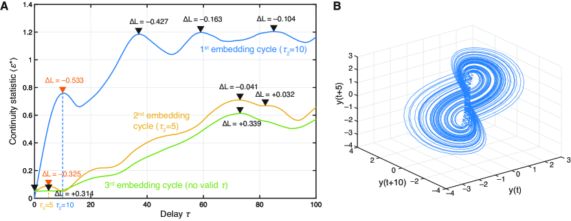
(1) For the actual reconstruction vectors $\vec{v}_{\text{act}}$, in each embedding cycle $\mathcal{D}_{d}$, $\langle\varepsilon^{\star}\rangle_{i}(\tau)$ is computed for all available $M$ time series $s_{i}(t)$. We comment on the procedure in the first embedding cycle $\mathcal{D}_{1}$ further below.
(2) We consider all those delays $\tau_{j}$ for each $\langle\varepsilon^{\star}\rangle_{i}(\tau)$, which correspond to local maxima $\hat{\tau_{j}}$ in $\langle\varepsilon^{\star}\rangle_{i}(\tau)$. These delays $\tau_{j}$ (and their corresponding time series $s_{i_{j}}(t)$) are used to build temporary reconstruction vectors $\vec{v}_{\text{temp}}(\tau_{j},s_{i_{j}})$, by concatenating $\vec{v}_{\text{act}}$ with the $\tau_{j}$-lagged time series $s_{i_{j}}(t)$.
(3) For each $\vec{v}_{\text{temp}}(\tau_{j},s_{i_{j}})$ and the actual reconstruction vectors $\vec{v}_{\text{act}}$ the $L$-statistic is simultaneous computed for many parameters $T_{M}$ (c.f. Fig. 4), and we denote them as $L_{\vec{v}_{\text{temp}}(\tau_{j},s_{i_{j}})}(T_{M})$ and $L_{\vec{v}_{\text{act}}}(T_{M})$. We compute the maximum $L$-decrease for $\vec{v}_{\text{temp}}(\tau_{j},s_{i_{j}})$ with respect to $\vec{v}_{\text{act}}$ as $\Delta L_{{\text{temp}}(\tau_{j},s_{i_{j}})}=\min\limits_{T_{M}}[L_{\vec{v}_{\text{temp}}(\tau_{j},s_{i_{j}})}(T_{M})-L_{\vec{v}_{\text{act}}}(T_{M})]$. This way $T_{M}$ is not a free parameter anymore.
(4) The delay-time series combination $(\tau_{j^{\prime}},s_{i_{j^{\prime}}}(t))$, which yields the minimum $\Delta L$ value will be picked for this embedding cycle $\mathcal{D}_{d}$, if $\Delta L<0$, and is used to construct the actual reconstruction vectors $\vec{v}_{\text{act}}=\vec{v}_{\text{temp}}(\tau_{j^{\prime}},s_{i_{j^{\prime}}})$ of dimension $d+1$
(5) $\vec{v}_{\text{act}}$ is passed into the next embedding cycle $\mathcal{D}_{d+1}$.
(6) We repeat steps (1) to (5) until we cannot minimize the $L$-statistic any further, i.e. when each considered potential embedding $\vec{v}_{\text{temp}}$ will yield a positive $\Delta L$. In this case the reconstruction cannot get any better and we stop. $\vec{v}_{\text{act}}$ constitutes the final reconstruction. Thus, the $L$-statistic provides a break criterion, without the introduction of any threshold parameter. Each embedding cycle ensures the maximum possible decrease of the cost-function.

Algorithm 1 Pecuzal Embedding

1:A uni- or multivariate dataset consisting of $M$ time series $s_{i}$ with same length and sampling and a range of possible delay values $\tau=0:\tau_{max}$

2:Normalize all $M$ time series to zero mean and unit variance

3:Set $\Delta L_{\text{min}}=-\text{inf}$

4:while $\Delta L_{\text{min}}<0$ do

5:     if 1st embedding cycle $\mathcal{D}_{1}$ then

6:         Compute $\langle\varepsilon^{\star}\rangle_{ik}(\tau)$ for all $M^{2}$ pairwise combinations of $s_{i},s_{k}$ for the given $\tau$’s

7:         for each peak $\hat{\tau_{j}}$ in each $\langle\varepsilon^{\star}\rangle_{ik}(\tau)$ do

8:              Create $\vec{v}_{\text{temp}}$ by appending the time series $s_{i}$ with the $\tau_{k}$-lagged time series $s_{k}$

9:              Compute the $L$-statistics for $\vec{v}_{\text{temp}}$ and $s_{i}$ for a range of parameter values $T_{M}=2:\tau_{max}$,

10:              denote them as $L_{\text{temp}}(T_{M})$ and $L_{s_{i}}(T_{M})$

11:              Compute $\Delta L_{\text{temp}}=\min\limits_{T_{M}}[L_{\text{temp}}(T_{M})-L_{s_{i}}(T_{M})]$

12:         end for

13:         From all $\Delta L_{\text{temp}_{j}}$ take the $\tau_{j}$, which corresponds to the peak with minimum $\Delta L$, $\Delta L_{\text{min}}$

14:         Save $\Delta L_{\text{min}}$ and $\vec{v}_{\text{temp}}$

15:     else if $\mathcal{D}_{d}$ then

16:         Compute $\langle\varepsilon^{\star}\rangle_{i}(\tau)$ for $\vec{v}_{\text{act}}$ and all $s_{i}$ for the given $\tau$’s

17:         for each peak $\hat{\tau_{j}}$ in each $\langle\varepsilon^{\star}\rangle_{i}(\tau)$ do

18:              Create $\vec{v}_{\text{temp}}$ by appending $\vec{v}_{\text{act}}$ with the $\tau_{i}$-lagged time series $s_{i}$

19:              Compute the $L$-statistics for $\vec{v}_{\text{temp}}$ and $\vec{v}_{\text{act}}$ for a range of parameter values $T_{M}=2:\tau_{max}$,

20:              denote them as $L_{\text{temp}}(T_{M})$ and $L_{\text{act}}(T_{M})$

21:              Compute $\Delta L_{\text{temp}}=\min\limits_{T_{M}}[L_{\text{temp}}(T_{M})-L_{\text{act}}(T_{M})]$

22:         end for

23:         From all $\Delta L_{\text{temp}_{j}}$ take the $\tau_{j}$, which corresponds to the peak with minimum $\Delta L$, $\Delta L_{\text{min}}$

24:         Save $\Delta L_{\text{min}}$ and $\vec{v}_{\text{temp}}$

25:     end if

26:     if $\Delta L_{\text{min}}<0$ then

27:         Set $\vec{v}_{\text{act}}=\vec{v}_{\text{temp}}$

28:     end if

29:end while

30:Set $\vec{v}_{\text{final}}=\vec{v}_{\text{act}}$

31:The final reconstruction vectors $\vec{v}_{\text{final}}$

We give some remarks on the proposed idea:

i) In case of the very first embedding cycle the actual reconstruction vectors $\vec{v}_{\text{act}}$ are not yet defined. Roughly speaking, the algorithm needs to find a time series to start with and which can act as the first component of the final reconstruction vectors. As explained in Algorithm 2, each of the available time series serves as $\vec{v}_{\text{act}}$ in the first run and consequently $M^{2}$ continuity statistics get computed in the first step, i.e., for each combination $(i,k)$ of the given time series $s_{i}(t)$. Note that we always use the unlagged available time series $s_{i}(t)$, which will constitute the first component of the reconstruction vectors, i.e. we set $\tau_{1}=0$. The continuity statistic reveals the correlation structure of its input, meaning that a lagged initial time series would lead to different consecutive delay values. However, the difference of the finally chosen delay values as well as the total time window of the reconstruction Tw$=\max(\tau_{1},\tau_{2},\ldots)$ would be identical, because the correlation structure does not change, at least in case of infinite data. Practically, any $\tau_{1}\neq 0$ only reduces the amount of data available and searching for the optimal $\tau_{1}$ in the sense of a minimal $\Delta L$ for the first embedding cycle $\mathcal{D}_{1}$ would increase the computation time tremendously.

ii) The $L$-statistic can not serve as an absolute measure, due to its dependence on the parameter $T_{M}$. Consider a time series and a potential 2-dimensional embedding consisting of this time series and a $\tau$-lagged version of it. This corresponds to the first embedding cycle $\mathcal{D}_{1}$ in Algorithm 2. Figure 4 shows the $L$-statistic for a range of parameters $T_{M}$ for the single time series and for the potential 2-dimensional reconstruction for two deterministic systems (panels A, B) and in case of the time series being uniformly distributed random numbers (panel C).

Figure 4: Illustration of the determination of $\Delta L$ within the embedding procedure for the first embedding cycle in a univariate case, using (A) the $y$-component of the Lorenz system (Appendix E.1), (B) the time series of the second node of a $N=8$ Lorenz 96 setup (Appendix E.2) and (C) 1,000 uniformly distributed random numbers. Shown are the $L$-statistics for the single time series (blue graphs) and a 2-dimensional embedding with a $\tau$-lagged version of itself (orange graphs) for a range of parameter values $T_{M}$. We set the number of nearest neighbours, which constitute a neighbourhood, necessary for computing the $L$-statistic, to $KNN=3$ and estimate $\tau$ from the first minimum of the corresponding auto-mutual information. The possible decrease of the $L$-statistic for this hypothetical embedding cycle with the chosen $\tau$ is simply $\Delta L(T_{M})=L_{\text{orange}}(T_{M})-L_{\text{blue}}(T_{M})$. When $\Delta L(T_{M})<0$ (shaded areas) the additional reconstruction vector component does increase the quality of the reconstruction, whereas when $\Delta L(T_{M})>0\leavevmode\nobreak\ \forall\leavevmode\nobreak\ T_{M}$ a further embedding is not beneficial. As expected that is the case for the stochastic signal in panel C. The Algorithm 2 automatically picks the first minimum $\Delta L$ over all $T_{M}$, which has also been the global minimum with respect to all $T_{M}$ throughout all examples we have considered so far.

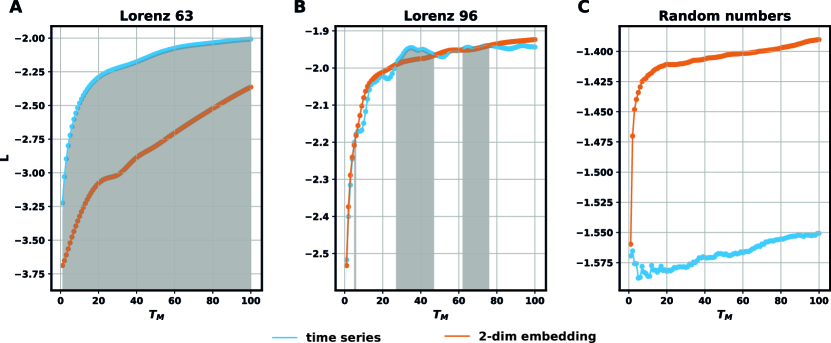
Whenever the $L$-statistic of the 2-dimensional reconstruction (orange graph) is lower than the one from the single time series (blue graph) an embedding would be beneficial (gray shaded areas in Fig. 4). But this is not always the case throughout the course of $T_{M}$ (see panel B). The conclusion is, that it is not meaningful to judge a reconstruction on a single $L$-value, gained from a fixed $T_{M}$. A reconstruction is always related to a function $L(T_{M})$ of the parameter $T_{M}$ and it is sensible to look at relative $L$-discrepancies between two consecutive embedding cycles, namely $\Delta L$. It turns out that some stochastic signals will yield a negative $\Delta L$ for $T_{M}=1$. In panel C of Fig. 4 this is not the case, but the proximity of the two curves only for $T_{M}=1$ is decernible. This is comprehensible by recalling that the $L$-statistic inherits the mean squared prediction error (see Eq. (17)), and a one-sample-prediction horizon is simply too short, to properly distinguish deterministic from stochastic sources. As a consequence we compute the $L$-statistics in each embedding cycle for $T_{M}$-values starting with $T_{M}=2$. Thus, for any embedding cycle each peak of the continuity statistic does not receive a certain absolute $L$-value, but rather a maximum possible decrease of $L$, $\Delta L$, with respect to the actual embedding (Fig. 3). Then one simply picks the peak, which yields the largest decrease. We can not rule out the possibility that we could obtain a lower overall decrease in $L$ for all embedding cycles by taking a different “path”, i.e. not go for the maximum decrease of $L$ in each embedding cycle. This would correspond to achieving a local minimum of the cost function in the parameter and embedding cycle space.

iii) We propose to stop the embedding process, when $\Delta L>0$ for all considered temporary reconstruction vectors $\vec{v}_{\text{temp}}$. One could think about incorporating a threshold, a small negative number, e.g. $\Delta L>-0.05$, to avoid only tiny decreases of the cost function encountered in an embedding cycle. Throughout all our computations this has not been necessary and, therefore, we dispense on such an additional parameter.

iv) The continuity statistic $\langle\varepsilon^{\star}\rangle$ itself contains information about the correlation structure of the data (cf. Sect. II.1), which makes it valuable in the context of an automated embedding procedure as proposed here, especially for multivariate input. Not only that the first maximum most often coincides with the value we would obtain from the first minimum of the mutual information, but the continuity statistic of two time series “levels off” at a certain value range. The absolute value of $\langle\varepsilon^{\star}\rangle$ represents the correlation structure of the data we are looking at and quantifies the independence from each other for a specific time lag. This fact allows our method to pick only time series from a multivariate set, which belong together, and, consequently, in combination with the corresponding decrease of the $L$-statistic, $\Delta L$, avoid stochastic signals (cf. Fig 4C, Table 1).

v) The time complexity of the proposed method is $\mathcal{O}(N\log{}N)$ as illustrated in Fig. 9 (Appendix A).

IV Application, Comparison & Results

We apply the proposed method to a range of different systems, artificial and experimental data, exemplifying its advantage over established methods. Specifically, we compare our method to the standard time delay embedding (TDE). We estimate the uniform delay $\tau$ by means of the first minimum of the auto-mutual information Fraser and Swinney (1986) and estimate the appropriate embedding dimension by using Cao’s method Cao (1997). Specifically, we automatically select the appropriate embedding dimension, when the $E_{1}$-statistic reaches the saturation value within a given threshold of the slope (we picked a slope of $<0.05$). We also look at two more sophisticated methods, which can also handle multivariate input, namely the method proposed by Garcia & Almeida (G&A) Garcia and Almeida (2005a, b); com (b) and Nichkawde’s method (MDOP) Nichkawde (2013). The latter mentioned methods do not come with a predefined way to terminate the embedding process. In order to terminate them we use Hegger’s Hegger and Kantz (1999) method of obtaining the optimal embedding dimension. Specifically, we set a FNN-threshold of 0.05, i.e., the algorithm breaks when the normalized fraction of FNN’s fall below this threshold in order to allow the algorithm to give meaningful results in the presence of noise. The threshold for the tolerable relative increase of the distance between the nearest neighbours, when increasing the embedding dimension is set to 2, as suggested in Hegger and Kantz (1999); Kennel et al. (1992). The threshold, which defines the factor of tolerable stretching for the $d_{E_{1}}$-statistic in case of G&A’s method is set to 10, as suggested by the authors. We estimate the decorrelation time by using the first minimum of the auto-mutual information and use it as the Theiler window Theiler (1986) in all approaches. In the multivariate input cases, we pick the maximum from all first minima of all auto-mutual information statistics. For distance computation, the Euclidean norm is used.

IV.1 Reconstruction evaluation statistics

In order to compare our approach with the established methods we need to quantify the goodness of the embedding. For this, we will consider six statistics. In addition to the overall decrease of the $L$-statistic, that is $\Delta L=\sum_{i=1}^{m-1}\Delta L_{i}$, where $m$ is the embedding dimension and $\Delta L_{i}$ the corresponding $L$-decreases in the encountered embedding cycles, we use two other statistics, which also reflect the neighbourhood relations of the reconstruction compared to the reference. One is the mutual false nearest neighbour statistic Rulkov et al. (1995). Instead of estimating the coupling strength/ degree of synchrony of two coupled oscillators, we use the statistic for assessing the similarity between the reference (time series gained from numerical integrations) and the reconstruction:

$$\text{MFNN}=\frac{1}{N}\sum_{i=1}^{N}\quad\frac{\sum_{k=1}^{K}|\vec{v}_{i}-\vec{v}_{i_{k}^{\text{ref}}}|}{\sum_{k=1}^{K}|\vec{u}_{i}-\vec{u}_{i_{k}^{\text{ref}}}|}\quad\frac{\sum_{k=1}^{K}|\vec{u}_{i}-\vec{u}_{i_{k}^{\text{rec}}}|}{\sum_{k=1}^{K}|\vec{v}_{i}-\vec{v}_{i_{k}^{\text{rec}}}|},$$ (4)

where $\vec{u}_{i}$ are the vectors of the reference/original system, $\vec{v}_{i},\leavevmode\nobreak\ i=1,\ldots,N$ the reconstruction vectors, $i_{k}^{\text{ref}}$ the indices of the $K$-nearest neighbours of index $i$ in the original system and $i_{k}^{\text{rec}},\leavevmode\nobreak\ k=1,\ldots,K$ the corresponding indices measured in the reconstruction. We propose the comparison of $K$ nearest neighbours instead of just focusing on the first nearest neighbour, in order to receive more robust results in the presence of noise. By sampling the data sufficiently high we allow the precise determination of quite large neighbourhoods of a fiducial point, so we set $K=10$ in our computations. The results vary in their absolute values with different choices of $K$, but the order of rank for the different test methods and their relative difference remain approximately constant. $\text{MFNN}=1$ corresponds to an ideal Afraimovich diffeomorphism Pecora et al. (1995); Afraimovich et al. (1986), higher values mark worse reconstructions. The other strict criterion we propose quantifies the degree of neighbourhood-relation conservation: the Joint Recurrence Rate Fraction (JRRF). It is based on the concept of a recurrence plot (RP), which is a 2-dimensional representation of a dynamical system as a binary matrix Eckmann et al. (1987); Marwan et al. (2007) (Appendix D). JRRF measures the accordance of the recurrence plot of the reference system, $\mathbf{R}^{\text{ref}}$, and the RP of the reconstruction, $\mathbf{R}^{\text{rec}}$).

JRRF $$=\frac{\sum_{i,j}^{N}JR_{i,j}}{\sum_{i,j}^{N}R_{i,j}^{\text{ref}}},\quad\text{JRRF}\in[0\leavevmode\nobreak\ 1]$$ (5)

$$\mathbf{JR} =\mathbf{R}^{\text{ref}}\circ\mathbf{R}^{\text{rec}}.$$ (6)

We compute both, $\mathbf{R}^{\text{ref}}$ and $\mathbf{R}^{\text{rec}}$, by fixing the recurrence threshold corresponding to a global recurrence rate of 8%. This is also to ensure comparability of the recurrence quantifiers described below Kraemer et al. (2018). Results a fairly similar for a wide range of choices of the recurrence rate we tried and the particular choice (in our case 8%) is not so important, since we apply them to all RP’s we compare. It is, of course, also possible to compare different recurrence plot quantifiers gained from $\mathbf{R}^{\text{rec}}$ to the ones derived from $\mathbf{R}^{\text{ref}}$ Marwan et al. (2007). We here choose the determinism (DET), the diagonal line length entropy (ENTR) and the recurrence time entropy (RTE) (Appendix D). The latter two are related to the Kolmogorov-Sinai-Entropy March et al. (2005); Baptista et al. (2010), but do not serve as straight forward estimators, when necessary corrections on the RP and its quantifiers are ignored Kraemer and Marwan (2019).

IV.2 Paradigmatic examples

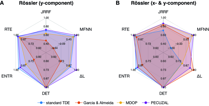
We investigate three paradigmatic chaotic systems, the Rössler system in the funnel regime (Appendix E.3), a driven Duffing oscillator in regular motion (Appendix E.3) and the Mackey-Glass delay equation (Appendix E.5). For all systems we compare the mean values of the evaluation statistics from ensembles of 1,000 trajectories with different initial conditions. Table 2 in Appendix B summarizes all results, also including uncertainties and results for 10% additive measurement noise. In order to easily compare the evaluation statistics, we use the relative deviation from the reference (e.g., $\frac{|DET^{\text{rec}}-DET^{\text{ref}}|}{DET^{\text{ref}}}$), except for the MFNN and the $\Delta L$-statistic, where we use the relative deviation from the best score (i.e., $\frac{|MFNN^{\text{rec}}-MFNN^{\text{best}}|}{MFNN^{\text{best}}}$). For a concise visual presentation we use spider plots in the following and plot 1 - rel. deviation, i.e. the closer to unity the value gets, the better the accordance to the reference or the best achieved value is.

(i) For the chaotic Rössler system, we reconstruct the state space for the univariate case (using the $y$-component, in order to allow TDE having the best chances Letellier and Aguirre (2002)) and for the multivariate case (using the $x$- and $y$-component). An overview over the results are shown in Figure 5. For TDE in the multivariate case we take the results from the univariate example, because TDE cannot handle multivariate input. Note that this leads to different relative values for MFNN and $\Delta L$, since we plot the deviation to the best score in these cases. The PECUZAL method performs best in the univariate as well as in the multivariate scenario, with improved outcomes for the multivariate one, as expected. This also holds in case of applied measurement noise, where our method even expands its lead for most measures (Table 2). Surprisingly, TDE also provides very good results in the univariate case and in the multivariate setup Garcia & Almeida’s method yields an overall larger deacrease of the $L$-statistic than PECUZAL, but only in the noise free case (see Table 2). This lower $\Delta L$ is not reflected in better performance of the other evaluation statistics. Specifically, the diagonal line length entropy values differ from the true reference value in the double-digit percentage range for G&A’s method.

Figure 5: (Relative) deviation of reconstruction by standard time delay embedding (TDE), the Garcia & Almeida (G&A), Nichkawde’s (MDOP), and PECUZAL methods, comparing the accordance of the RPs of the reconstructed attractor and the reference attractor (JRRF), mutual false nearest neighbors (MFNN), $\Delta L$-statistic, as well as the recurrence quantifiers determinism (DET), diagonal line length entropy (ENTR), and the recurrence time entropy (RTE). (A) Univariate case using the $y$-component of the numerically integrated Rössler system (Appendix E.3) and (B) multivariate case using the $x$- and $y$-values of the Rössler system. Since TDE cannot handle multivariate input we take the values from the univariate case here for illustrative reasons, which result in different relative values in case of MFNN and the $\Delta L$-statistic. For these measures we plot the 1- relative deviations to the best score, which increases in the multivariate case. For the other statistics we plot 1- relative deviations to the reference score, i.e. the closer to unity the value gets, the better the accordance to the reference or the best achieved value is.

Figure 6: Same as Fig. 5, here for the Duffing system (Appendix E.4).

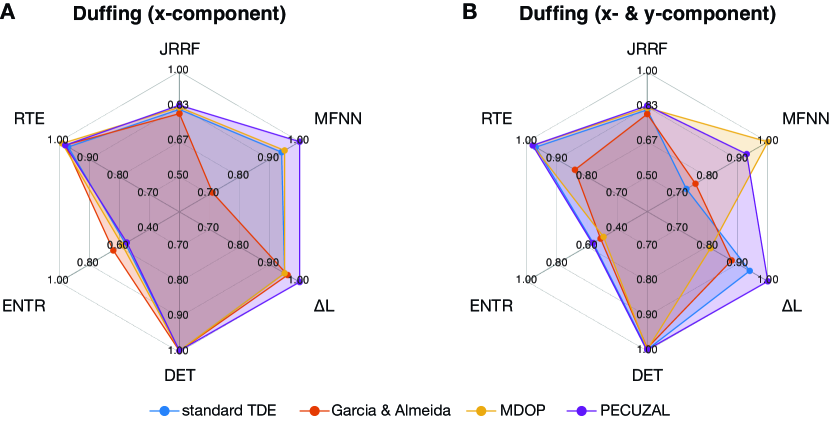
(ii) The overall rating also holds for the driven Duffing oscillator (Fig. 6), but there are severe differences. In contrast to the chaotic Rössler system here it seems that the additional given time series for the multivariate scenario do not improve the reconstructions significantly. The JRRF do not get better and remain on a quite high level of 80% (G&A) up to 84% (PECUZAL) accordance with the reference recurrence plot $\mathbf{R}^{\text{ref}}$. This is also reflected in the $\Delta L$ statistic, which also does not improve in the multivariate case for G&A and MDOP, and only slightly decreases for PECUZAL. The same story is told by looking at the other evaluation statistics summarized in Table 2. It is important to note that under noise our proposed method outperforms the others in almost all cases, but in principle we notice that the signal to noise ratio seems to be very low and biases the results of all methods more than in case of the Rössler example. Specifically in case of RTE deviations to the true reference value increase from the low single digit percentage range up to 62% in the noisy case. The reason is that in regular motion we expect a near zero value of RTE and noise easily blurrs the diagonal lines in the recurrence plot, leading to a broader distribution of recurrence times and, thus, to randomly elevated RTE values. The very same problem make the ENTR values deteriorate for all methods, here already apparent in the noise free case. In a regular motion system ENTR is biased the most when no correction of the diagonal lines is performed, which has been shown by Kraemer and Marwan (2019). The proposed skeletonizaton of the recurrence plots for the purpose of reducing the bias in the diagonal line based recurrence plot quantifiers, such as ENTR and RTE, lead to way better results in the one digit percentage range even for noise, as expected. Due to the computational complexity of the skeletonization algorithm Kraemer and Marwan (2019) we did not apply this correction scheme to all of the 1,000 runs in this experiment, but rather tried it on small samples not shown here, in order to understand the bad performances for all methods in case of ENTR and RTE.

(iii) In contrast to the above systems, the Mackey-Glass system (Appendix E.5) is infinite dimensional and we have do deal with a univariate time series from the numerical integration, which is why we do not have a “reference” value we could base our computations on. Therefore, we can only use the $\Delta L$-statistic (Table 2). The proposed PECUZAL method performs significantly better than the other methods with Garcia & Almeida’s method coming second, especially in the presence of noise. Here all methods but the proposed one yield reconstructions with corresponding positive $\Delta L$-values, i.e. the suggested embeddings do not decrease the overall $L$-statistic. Admittedly, PECUZAL also comes with a very small negative $\Delta L$ value, with 0 falling within the $1\sigma$-interval. This finding indicates a too low signal to noise ratio, which we comment on below. Farmer (1982) conjectured a linear relation between the delay chosen in the Mackey-Glass equation and the corresponding dimensionality of the attractor (c.f. Table I in Farmer (1982)). A linear fit to the data of that table suggests an attractor-dimension of $d_{A}\approx 5.3$ with the 95% confidence interval being between $\approx 2.1773$ and $\approx 8.2888$. The studied methods give $5\pm 0\leavevmode\nobreak\ (6.7\pm.5)$ (TDE), $3\pm 0\leavevmode\nobreak\ (4.6\pm 1)$ (G&A), $4\pm 0\leavevmode\nobreak\ (2\pm 0)$ (MDOP) and $7\pm 0\leavevmode\nobreak\ (2.2\pm 1.7)$ (PECUZAL). The bracketed values correspond to the case of 10% additive noise. While all methods meet Farmer’s conjecture in the noise free scenario, this does not hold for the MDOP method an the proposed method in the noisy case. Both methods suggest too low embedding dimensions. This is due to the fact that the signal to noise ratio is apparently too low and PECUZAL treats the signal as a stochastic source for some realizations where it does not embed the data at all, while it did not do it in case of the Rössler and Duffing system, despite the same variance of the white Gaussian noise. Results from G&A and TDE do fall in the 95% confidence interval, which is large, because of the weak data basis given in Ref.Farmer (1982)) and the resulting uncertain fit. We find the time window of the embedding, i.e., the total time span covered by a reconstruction vector, decreasing with increasing noise level throughout our experiments. This is very much in line with the findings of Ragwitz and Kantz (2002).

We finally look at two made up, ill-defined multivariate datasets, in order to see how the G&A, MDOP, and the PECUZAL method cope with redundant data and with stochastic signals.

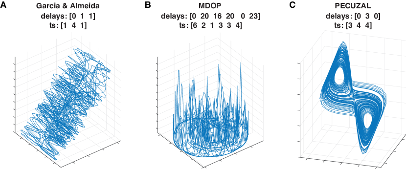
(i) First we construct a dataset consisting of six time series (Fooling dataset I). The first two time series are the $x$- and $y$-component of the Rössler system (Appendix E.3), the third and fourth time series are the $x$- and $y$-component of the Lorenz system (Appendix E.1), the fifth time series corresponds to $x_{\text{R\"{o}ssler}}^{2}+y_{\text{R\"{o}ssler}}$, whereas the sixth time series is set to $x_{\text{Lorenz}}\cdot y_{\text{Lorenz}}+y_{\text{Lorenz}}$. Our proposed method does not mix time series from both systems and sticks to one system (Lorenz in this case) (Tab. 1). It suggests a 3-dimensional embedding and also does not need the redundant information stored in the fifth and the sixth time series of the input dataset. In contrast, G&A and MDOP fail here, suggesting a 3-dimensional and a 6-dimensional embedding, respectively, mixing up the different systems yielding a useless reconstruction (Fig. 7).

(ii) The second made-up dataset (Fooling dataset II) consists of three time series of length 5,000, with the first one being an auto-regressive process of order 1 with parameters (0, 0.9) and initial condition $u_{0}=0.2$, to mimic coloured noise. The second and third time series are Gaussian and uniform random numbers. While G&A and MDOP embed the non-deterministic time series, our proposed algorithm suggests no embedding and throws an error (Tab. 1). The reason is, that the $L$-statistic is a monotonically increasing function of the embedding dimension for stochastic data for any prediction horizon parameter $T_{M}$, i.e., the algorithm cannot minimize $L$ already in the first embedding cycle. For the sake of completeness we have to stress that this particular example should not be read as a claim of a generalizable behaviour of our proposed method to deal with auto-regressive processes of arbitrary order $p$. In the case of higher-order AR processes, PECUZAL often suggests an embedding with a dimension that corresponds to the order of the AR process, as we would expect it theoretically. We have noticed, however, that the embedding depends heavily on the length of the time series used, which is in line with the findings of Holstein and Kantz (2009), but also of the choice of the particular AR-parameters and the order of the AR process under study. A systematic consideration of PECUZAL’s embedding suggestions for this class of processes is beyond the scope of this paper.

Figure 7: Reconstructions of the Fooling dataset I (see text for details). In case of the MDOP method (panel B), we plot the first three components of the 6-dimensional trajectory. While G&A and MDOP methods mix timeseries from different systems, leading to nonsensical reconstructions (panels A and B), our proposed method (panel B) sticks to time series from one system (Lorenz in this case).

Table 1: Embedding dimension, the accordingly chosen time series and corresponding time lags for the fooling datasets, mimicking mixed deterministic data from different systems and redundant time series as well as stochastic time series. We compare Garcia & Almeida’s (G&A), Nichkawde’s (MDOP), and our proposed PECUZAL method.

	m			chosen time series			Delay’s
System	G&A	MDOP	PECUZAL	G&A	MDOP	PECUZAL	G&A	MDOP	PECUZAL
Fooling dataset I	3	6	3	1, 4, 1	6, 2, 1, 3, 3, 4	3, 4, 4	0, 1, 1	0, 20, 16, 20, 0, 23	0, 3, 0
Fooling dataset II	6	6	—	1, 2, 2, 1, 1, 1	3, 3, 1, 2, 2, 1	—	0, 1, 2, 3, 2, 1	0, 1, 0, 1, 0, 1	-

IV.3 Experimental data

We will now utilize the PECUZAL embedding method on experimental data. Specifically, we look at a chaotic time series from electrochemical oscillations. The experiment was performed with the chaotic electrodissolution of nickel in sulfuric acid Kiss et al. (2000). A standard three-electrode electrochemical cell was used with a 1-mm diameter nickel wire as working, a Pt counter, and a $\textrm{Hg/Hg}_{2}\textrm{SO}_{4}/\textrm{sat.\leavevmode\nobreak\ K}_{2}\textrm{SO}_{4}$ reference electrode. The electrolyte was 4.5 M $\textrm{H}_{2}\textrm{SO}_{4}$ at 10°C. The nickel wire was connected to the working point of the potentiostat through an individual resistance ($R_{\textrm{ind}}$), and a potentiostat (Gill AC, ACM Instruments) applied a constant circuit potential ($V_{0}$, with respect to the reference electrode). At a given circuit potential, the rate of the metal dissolution, measured as the current, can exhibit chaotic oscillations due the hidden negative differential resistance and additional nonlinear processes related to the passivation kinetics Wickramasinghe and Kiss (2010). About 500 current oscillations were recorded at a data acquisition rate of 200Hz, which corresponds to about 200 points per cycle and a time series length of $N=100,000$. There are two primary bifurcation parameters in the experiment: the individual resistance, which affects the charging time constant of the electrical double layer, and the circuit potential, which drives the dissolution. We consider a setting with $R_{\textrm{ind}}$ = 1.5 k$\Omega$ and $V_{0}$ = 1,360 mV.

Figure 8: (A) Entire z-standardized and downsampled time series from electrochemical oscillations of length $N=50,000$ and (B) a sub-sample of length $\hat{N}=2,500$. (C) The relative deviation of the medians of the distributions of the RQA-quantifiers ENTR, LAM, RTE and $\mathcal{T}$ obtained from RPs of $1,000$ sub-samples to their reference values obtained from RPs of the entire time series for the four reconstruction methods.

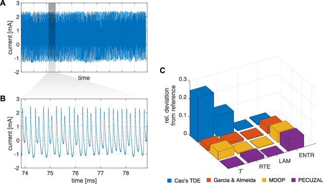
We demonstrate the ability of the proposed embedding method to cope with rather small to intermediate sized experimental datasets. We first downsample the time series to $N=50,000$ (Fig. 8A). Reconstructions for the four methods (TDE, G&A, MDOP, PECUZAL) are then computed from which we obtain RPs (with a fixed recurrence rate of 8%, in order to guarantee comparability) and the corresponding RQA-quantifiers diagonal line length entropy (ENTR), the laminarity (LAM), the recurrence time entropy (RTE) and the recurrence network measure transitivity ($\mathcal{T}$), see Appendix D. We denote each of these values for each of the reconstruction method as its reference values. We then repeat the described procedure for $1,000$ sub-samples of length $\hat{N}=2,500$ drawn from the time series at random (shown exemplary in Fig. 8B), i.e. for each of the $1,000$ sub-samples we compute the reconstruction for each of the four methods, its corresponding RP and the RQA-quantifiers. This will result in distributions for ENTR, LAM, RTE and $\mathcal{T}$ for each reconstruction method. Finally we compare the medians of these distributions to their reference values and plot the relative deviation $\frac{|\text{RQA}_{\text{median(distr.)}}-\text{RQA}_{ref}|}{\text{RQA}_{ref}}$ in Fig. 8C. The capability of the four methods to allow for satisfying estimates from short time series samples differs strongly for the different RQA-quantifiers. The largest discrepancies to the reference can be noted for TDE in case of $\mathcal{T}$ and RTE. For LAM all methods estimate the reference very well from the subsamples. While our proposed method slightly comes last in case of ENTR, it yields the best results for $\mathcal{T}$ and LAM and is performing well in case of RTE. The example shown here can not be generalized, but it underpins our claim that PECUZAL provides robust state space reconstructions for a very broad range of processes under different conditions, which are often better, but always at least equally well than the ones obtained from the established methods.

V Conclusions

A fully automated approach for state space reconstruction from uni- or even multivariate time series is proposed and compared to established methods. The algorithm works iteratively and appends the reconstruction vectors in each embedding cycle with an appropriate time delay and an according time series until a cost function cannot be minimized further. Its core functionality is based on identifying potential time delays and its corresponding time series in each embedding cycle by using the continuity statistic. For each of those delays, temporary reconstruction vectors are build and the cost function is computed. The delay value, which yields the maximum decrease of the cost function is selected. If none of the considered delay values yields a decrease of the cost function the reconstruction can not get any better and the final embedding is obtained without the need of setting any threshold parameter. Usually the time delays chosen that way are not simply multiples of each other, but rather reflect even complex correlation structures within the data. This is why the algorithm is also able to detect time series stemming from a stochastic source, which it will not embed. Except from computing the decorrelation time of the data for providing a valid Theiler window for the nearest neighbour search, and providing a range of possible delay values the algorithm shall encounter, there are neither any data preprocessing steps necessary, nor any free parameters need to be adjusted before using the proposed routine. The approach is demonstrated on a variety of exemplary systems as well as on experimental data stemming from chaotic chemical oscillators. We find that it provides often better, but always at least equally well reconstructions than the established methods. It is furthermore capable of providing meaningful reconstructions for rather short time series, which particularly holds for the case of multivariate input. The additional computational effort in comparison to standard time delay embedding is manageable and justified. Since the proposed method works automatically, is basically parameter free, and can handle multivariate input without mixing data originating from different systems, we can think of a wide range of potential applications. This is especially true for scenarios, where multiple sensors or channels of a detector monitor real world processes, which are not isolated observables, i.e., in engineering, earth- and life science contexts. The provided software (Appendix A) in three common coding languages will facilitate the use of the presented method.

Appendix A Implementation and code availability

The study that we present here is available as a fully reproducible code base Kraemer and Datseris (2021). In addition, we have implemented performant versions of the embedding algorithms, as well as the automated pipeline for optimal embedding. A single package is provided for Python Kraemer and Marwan (2021a) (https://pypi.org/project/pecuzal-embedding/) and a toolbox for MATLAB^® Kraemer and Marwan (2021b),
(https://de.mathworks.com/matlabcentral/fileexchange/86004-pecuzal-embedding-algorithm-for-matlab) while for the Julia language we have integrated the PECUZAL algorithm into the library DynamicalSystems.jl Datseris (2018) (the other methods “TDE, Garcia&Almedia, MDOP” were already part of the library). The automated pipeline for optimal embedding has been further refined for better user experience and is also part of DynamicalSystems.jl.

Figure 9: Median time complexity for the state space reconstruction from the $y$-component of the Rössler system (Appendix E.3) for TDE, Garcia & Almeida’s, MDOP, and PECUZAL method. Ensembles of function calls for each considered time series length $N$ are computed and the median values are shown (implemented in BenchmarkTools.jl Chen and Revels (2016)). A Theiler window is set as the first minimum of the auto-mutual information and the maximum encountered time delay is set to four times the Theiler window for TDE, G&A, and PECUZAL.

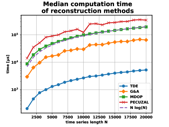
The Julia versions of the algorithms have been heavily optimized and are the most performant ones by orders of magnitude in parts, when compared to the Python (and MATLAB^®) implementation. Due to the nearest neighbour tree search, all compared methods have $\mathcal{O}(N\log{}N)$ time complexity (Fig. 9). Our proposed method is slightly (but consistently) slower than the established methods, with standard time delay embedding performing best (Cao’s method). Worth mentioning is the fact that in the MDOP case the most computational effort is put on the estimation of the maximum considered delay value and not on the computation of their $\beta$-statistic. Considering that an optimal embedding is a one-time operation, we believe that all methods shown here are practically useful with respect to their computational complexity.

Appendix B Numerical Results

Chaotic Rössler system, driven Duffing oscillator in regular motion, and nonlinear time-delay Mackey-Glass equation are used to evaluate the performance of the different embedding approaches (TDE, G&A, MDOP, and PECUZAL). We consider univariate and multivariate embedding (Rössler and Duffing). The $y$-component of the Rössler system and the $x$-component of the Duffing system are used for the univariate embedding, wheres the $x$- and $y$-values of the corresponding systems are used for the multivariate embedding. For the TDE only univariate embedding is possible and, thus, there are no results for the multivariate case.

Ensembles of 1,000 trajectories using different initial conditions are used. Additionally, we consider additive noise with an amplitude of 10% of the standard deviation of the corresponding signal.

All RPs are computed using a fixed recurrence rate of 8% and a minimum line length of 2.

Table 2: Results of the evaluation measures: accordance of the recurrence plot (JRRF), mutual false nearest neighbors (MFNN), $\Delta L$-statistic, as well as the recurrence quantifiers determinism (DET), diagonal line length entropy (ENTR), and recurrence time entropy (RTE) for the standard time delay embedding (TDE), Garcia & Almeida (G&A), Nichkawde’s (MDOP), and PECUZAL-method (see text for details), using chaotic Rössler system, driven Duffing oscillator in regular motion (both in univariate (u) and multivariate (m) case), and nonlinear time-delay Mackey-Glass equation. Mean values and standard deviation of ensembles consisting of 1,000 integrated trajectories are shown. Bracketed values present results for additive noise. The results of recurrence quantifiers are presented as relative deviations from the reference. The best results for each considered system are highlighted in black.

JRRF

MFNN

$\Delta L$

System

TDE

G&A

MDOP

PECUZAL

TDE

G&A

MDOP

PECUZAL

TDE

G&A

MDOP

PECUZAL

Rössler (u)

$.71\pm.02$

$.48\pm.04$

$.64\pm.01$

$.73\pm.01$

$3.8\pm.3$

$8.7\pm 2.4$

$4.0\pm.4$

$3.3\pm.2$

$-1.27\pm.09$

$-1.03\pm.17$

$-1.24\pm.08$

$-1.41\pm.08$

($.71\pm.02$)

($.6\pm.03$)

($.62\pm.01$)

($.73\pm.01$)

($4.1\pm.3$)

($5.1\pm.6$)

($4.8\pm.4$)

($3.7\pm.2$)

($-1.14\pm.05$)

($-0.94\pm.08$)

($-0.95\pm.04$)

($-1.23\pm.05$)

Rössler (m)

—

$.83\pm.02$

$.86\pm.04$

$.87\pm.01$

—

$1.9\pm.6$

$1.4\pm.1$

$1.29\pm.08$

—

$-1.58\pm.2$

$-1.26\pm.12$

$-1.48\pm.08$

—

($.82\pm.04$)

($.87\pm.01$)

($.87\pm.01$)

—

($2.4\pm.6$)

($1.57\pm.06$)

($1.5\pm.1$)

—

($-1.14\pm.09$)

($-1.04\pm.07$)

($-1.28\pm.04$)

Mackey-G

—

—

—

—

—

—

—

—

$-.43\pm.0$

$-.57\pm.0$

$-.35\pm.0$

$-.77\pm.0$

—

—

—

—

—

—

—

—

($.12\pm.04$)

($.12\pm.07$)

($1\times 10^{7}\pm.0$)

($-0.02\pm.03$)

Duffing (u)

$.82\pm.01$

$.80\pm.04$

$.83\pm.02$

$.84\pm.02$

$4.0\pm 1.2$

$4.9\pm 1.7$

$3.9\pm.9$

$3.8\pm.8$

$-1.66\pm 1.7$

$-1.68\pm.18$

$-1.66\pm.16$

$-1.75\pm.15$

($.74\pm.01$)

($.63\pm.04$)

($.69\pm.02$)

($.73\pm.02$)

($8.9\pm.4$)

($10.2\pm 1.6$)

($8.8\pm.3$)

($15.1\pm 3.7$)

($-.5\pm.05$)

($-.51\pm.08$)

($-.41\pm.06$)

($-.69\pm.04$)

Duffing (m)

—

$.80\pm.06$

$.83\pm.02$

$.84\pm.02$

—

$3.9\pm 1.5$

$3.1\pm.8$

$3.3\pm.9$

—

$-1.6\pm.2$

$-1.4\pm.2$

$-1.8\pm.2$

—

($.72\pm.04$)

($.74\pm.02$)

($.73\pm.01$)

—

($10.0\pm 1.8$)

($7.9\pm.6$)

($14.1\pm 3.9$)

—

($-.5\pm.1$)

($-.3\pm.1$)

($-.71\pm.04$)

	DET ($\times 10^{3}$)				ENTR				RTE
System	TDE	G&A	MDOP	PECUZAL	TDE	G&A	MDOP	PECUZAL	TDE	G&A	MDOP	PECUZAL
Rössler (u)	$.03\pm.01$	$.71\pm.28$	$.03\pm.01$	$.01\pm.01$	$.05\pm.01$	$.32\pm.03$	$.18\pm.01$	$.08\pm.01$	$.03\pm.01$	$.07\pm.02$	$.07\pm.01$	$.04\pm.01$
	($6.6\pm.8$)	($7.2\pm 1.2$)	($8.0\pm.7$)	($3.0\pm.4$)	($.14\pm.02$)	($.05\pm.03$)	($.08\pm.02$)	($.08\pm.01$)	($.02\pm.01$)	($.04\pm.01$)	($.04\pm.01$)	($.02\pm.01$)
Rössler (m)	—	$.95\pm.35$	$.19\pm.06$	$.14\pm.03$	—	$.2\pm.04$	$.09\pm.02$	$.08\pm.02$	—	$.06\pm.02$	$.02\pm.01$	$.01\pm.01$
	—	($6.6\pm 2.4$)	($4.9\pm.4$)	($2.8\pm.3$)	—	($.05\pm.03$)	($.08\pm.01$)	($.06\pm.01$)	—	($.02\pm.01$)	($.01\pm.01$)	($.01\pm.0$)
Duffing (u)	$3.9\pm.08$	$3.6\pm 1.0$	$4.1\pm.3$	$4.2\pm.3$	$.44\pm.09$	$.36\pm.07$	$.42\pm.02$	$.45\pm.05$	$.03\pm.04$	$.02\pm.03$	$.01\pm.01$	$.02\pm.02$
	($97.4\pm 4.3$)	($113.8\pm 14.2$)	($113.4\pm 15.4$)	($61.5\pm 5.7$)	($.03\pm.02$)	($.30\pm.06$)	($.37\pm.05$)	($.21\pm.09$)	($.62\pm.01$)	($.32\pm.16$)	($.54\pm.03$)	($.46\pm.06$)
Duffing (m)	—	$8.3\pm 19$	$4.2\pm.3$	$4.2\pm.3$	—	$.49\pm.12$	$.51\pm.07$	$.44\pm.06$	—	$.16\pm.57$	$.02\pm.02$	$.02\pm.03$
	—	($113\pm 18$)	($103\pm 10$)	($61\pm 4$)	—	($.32\pm.07$)	($.22\pm.07$)	($.22\pm.08$)	—	($.56\pm.09$)	($.61\pm.01$)	($.44\pm.06$)

Appendix C Dependency on parameters

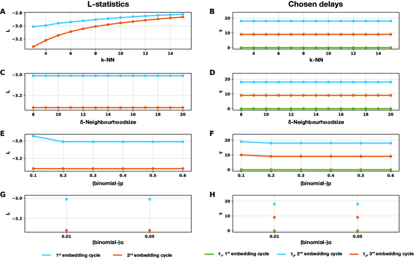
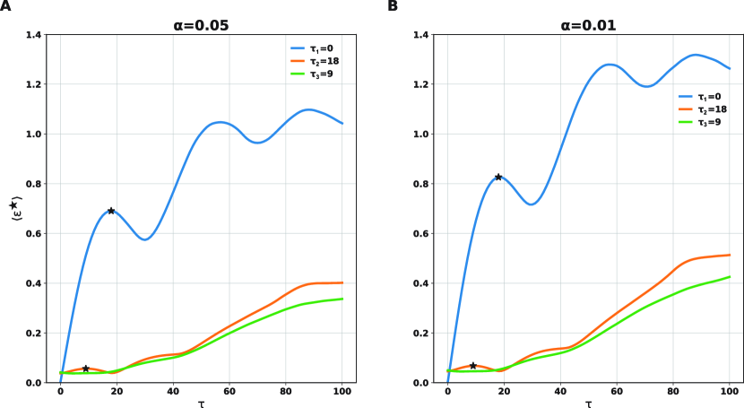
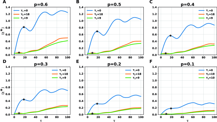
We investigate the impact of different parameter settings on the resulting reconstruction of our proposed method for the $x$-component of the Lorenz system (Appendix E.1). In particular, Figure 10) shows the sensitivity of the $L$-statistic value and the chosen delays with respect to the number of nearest neighbours $kNN$ for a fixed paramter $T_{M}=20$ (panels A, B) and also the dependence on the continuity statistic parameters $\delta$-Neighborhoodsize (panels C, D), the (binomial) probability $p$ (panels E, F) and significance-level $\alpha$ (panels G, H). The critical dependence of the $L$-statistic on the parameter $T_{M}$ is discussed in Sect. III and Fig. 4. The results show very little impact on the reconstruction quality and, thus, confirm our choice of fixed parameter values for the algorithm. Specifically, the crucial qualitative course of the continuity statistic, i.e., the position of the local maxima, remains unchanged for relevant choices of $\alpha$ and in the vicinity of $p=0.5$, which is the proposed fixed value (Figs. 11 and 12).

Figure 10: $L$-statistic (left panels) and chosen delays (right panels) for a variety of choices of parameters for embedding the Lorenz system, relevant for the PECUZAL method. See text for details. When not varied, the other parameters were fixed to $\delta$-Neighbourhoodsize$=14$, $p=0.5$, $\alpha=0.05$ and $kNN=3$, as we propose.

Figure 11: Impact of different significance-level choices $\alpha$ on the continuity statistic. The other parameters for obtaining the continuity statistic were fixed to $\delta$-Neighbourhoodsize$=14$ and $p=0.5$.

Figure 12: Impact of different choices of the binomial probability parameter $p$ on the continuity statistic. The other parameters for obtaining the continuity statistic were fixed to $\delta$-Neighbourhoodsize$=14$ and $\alpha=0.05$.

Appendix D The recurrence plot and its quantification measures

A recurrence plot (RP) is a binary, square matrix $\mathbf{R}$ representing the recurrences of states $\vec{x}_{i}$ ($i=1,\ldots,N$, with $N$ the number of measurement points) in the $d$-dimensional state space Eckmann et al. (1987); Marwan et al. (2007)

$${R}_{i,j}(\varepsilon)=\Theta\left(\varepsilon-\|\vec{x}_{i}-\vec{x}_{j}\|\right),\qquad\vec{x}\in\mathbb{R}^{d},$$ (7)

with $\|\cdot\|$ a norm, $\varepsilon$ a recurrence threshold, and $\Theta$ the Heaviside function. There are several ways to quantify the structures and dynamics encoded therein, but here we look at the determinism Webber, Jr. and Zbilut (1994), which is the fraction of recurrence points that form diagonal lines of length $\ell$

$$\text{DET}=\frac{\sum_{\ell=\ell_{\min}}^{N}P(\ell)}{\sum_{\ell=1}^{N}\ell P(\ell)},$$ (8)

with $P(\ell)$ being the histogram of all diagonal line lengths in the RP and $\ell_{\min}$ the considered minimal line length (here set to 2). Another quantifier is the Shannon entropy of the probability distribution $p(\ell)=\frac{P(\ell)}{\sum_{\ell}P(\ell)}$ to find a diagonal line of exact length $\ell$

$$\text{ENTR}=-\sum_{\ell=\ell_{\min}}^{N}p(\ell)\ln p(\ell).$$ (9)

It is also possible to look at the Shannon entropy of the length distribution of the white vertical lines $\ell_{\text{w}}$, which correspond to recurrence times

$$\text{RTE}=-\sum_{\ell_{\text{w}}=1}^{N}p(\ell_{\text{w}})\ln p(\ell_{\text{w}}).$$ (10)

Analogue to the definition of the determinism, the laminarity is the fraction of recurrence points that form vertical lines

$$\text{LAM}=\frac{\sum_{\ell_{\text{v}}=\ell_{\text{v},\text{min}}}^{N}P(\ell_{\text{v}}v)}{\sum_{\ell_{\text{v}}=1}^{N}\ell_{\text{v}}vP(\ell_{\text{v}}v)},$$ (11)

with $\ell_{v}$ the length of a vertical line, $P(\ell_{\text{v}}v)$ the histogram of all vertical lines in the RP and $\ell_{\text{v},\text{min}}$ the considered minimal line length (here set to 2).

Finally, the RP can be considered as the adjacency matrix of an $\varepsilon$-recurrence network Zou et al. (2019), $\mathbf{A}=\mathbf{R}-\mathbb{1}$ and define the transitivity Boccaletti et al. (2006) as

$$\mathcal{T}=\frac{\sum_{i,j,k=1}^{N}A_{jk}A_{ij}A_{ik}}{\sum_{i,j,k=1}^{N}A_{ij}A_{ik}(1-\delta_{jk})},$$ (12)

which is a measure characterising the geometric structure of the state space attractor Donner et al. (2011).

Appendix E Exemplary models

The models described in the following are all integrated using DynamicalSystems.jl and DifferentialEquations.jl Datseris (2018); Rackauckas and Nie (2017) in the Julia Language.

E.1 Lorenz system

The Lorenz system Lorenz (1963) is defined as

$$\dot{x} =\sigma(y-x)$$

$$\dot{y} =x(\rho-z)-y$$

$$\dot{z} =xy-\beta z.$$

We set the initial condition to $u_{0}=[1.0,1.0,50.0]$, use a sampling time of $\Delta t=0.01$ and discard the first 1,000 points of the integration as transients. For producing Fig. 3 we set the parameters to $\sigma=10,\beta=8/3,\rho=60$ and use a time series consisting of 5,000 samples. In Figs. 4, 10, 11, 12 and the redundancy fooling-dataset in section IV.2 we use the standard parameter values $\sigma=10,\ \beta=8/3,\ \rho=28$ and also a time series consisting of 5,000 samples.

E.2 Lorenz 96 system

The Lorenz 96 system Lorenz (1995) is defined as

$$\frac{dx_{i}}{dt}=(x_{i+1}-x_{i-2})x_{i-1}-x_{i}+F$$

with $x_{i}$ the state of the system for nodes $i=1,\dots,N$ and it is assumed that the total number of nodes is $N\geq 4$. The forcing constant $F$ serves as the control parameter. Here we set $N=8$, $F=4.472$ and the initial condition to $u_{0}=[0.590;0.766;0.566;0.460;0.794;0.854;0.200;0.298]$, use a sampling time of $\Delta t=0.1$ and discard the first 2,500 points of the integration as transients leaving us with a time series consisting of 5,000 samples.

E.3 Rössler system

The Rössler system Rössler (1976) is defined as

$$\dot{x} =-y-z$$

$$\dot{y} =x+ay$$

$$\dot{z} =b+z(x-c).$$

We randomly choose the initial conditions uniformly from an interval $[0,\,2]$ and discard the first 2,000 points of the integration as transients working with time series of length $N=10,000$ (for Fig. 9 we set $N=20,000$). The parameters are set to $a=0.2925,\ b=0.1,\ c=8.5$ (funnel regime) for the experiment in Sect. IV.2, where the sampling time is set to $\Delta t=0.03$ and $a=0.2,\ b=0.2,\ c=5.7$ with a sampling time of $\Delta t=0.02$ elsewhere.

E.4 Driven Duffing oscillator

The driven Duffing/Van der Pol oscillator Duffing (1918); Appleton and van der Pol junr. (1922) is defined as

$$\dot{x} =y$$

$$\dot{y} =\mu(1-x^{2})y-\alpha x-\beta x^{3}+z$$

$$\dot{z} =\gamma\cdot\omega\cdot\cos(\omega\cdot t),$$

with $\mu=0.1,\ \alpha=1,\ \beta=0,\ \gamma=0.5,$ and $\omega=2$ Cui et al. (2018) resulting in a regular, quasi periodic motion. We randomly choose the initial conditions $x_{0},\ y_{0},\ z_{0}$ uniformly from the interval $[0,\,0.2]$, use a sampling time of $\Delta t=0.1$ and discard the first 2,000 points of the integration as transients, resulting in time series of length $N=5,000$.

E.5 Mackey-Glass equation

The Mackey-Glass equation Mackey and Glass (1977) is the nonlinear time delay differential equation

$$\dot{x}=\beta\frac{x_{\tau}}{1+x^{n}}-\gamma x,$$

with the lag $\tau=44$, and the parameters $n=10$, $\beta=0.2$, and $\gamma=0.1$. $x_{\tau}$ represents the value of $x$ at time $t$-$\tau$. We randomly choose the initial conditions uniformly from an interval $[0,\,1.5]$, use a sampling time of $\Delta t=0.5$ and discard the first 2,000 points of the integration as transients, resulting in time series of length $N=10,000$.

Appendix F Details of the $L$-statistic

The concept of quantifying noise amplification in the context of the validation of an attractor reconstruction has been proposed in Casdagli et al. (1991). The reconstruction process is considered in the presence of noise and the finite data availability as a modeling problem, introducing a noise amplification and estimation/prediction error for any measures on the reconstructed attractor. The variance of the conditional probability density function is a “natural criterion for assessing predictability” Casdagli et al. (1991) and is used as the noise amplification for a fiducial point $\vec{v}_{\text{fid}}(t)$ at a given noise level $\varepsilon$ on the reconstruted attractor

$$\sigma_{\varepsilon}\bigl{(}T,\vec{v}_{\text{fid}}(t)\bigr{)}=\frac{1}{\varepsilon}\sqrt{Var\Bigl{(}\vec{v}\bigl{(}t+T\bigr{)}|B_{\varepsilon}\bigl{(}\vec{v}_{\text{fid}}(t)\bigr{)}\Bigr{)}},$$ (13)

with $Var\Bigl{(}\vec{v}\bigl{(}t+T\bigr{)}|B_{\varepsilon}\bigl{(}\vec{v}_{\text{fid}}(t)\bigr{)}\Bigr{)}$ being the conditional variance of $\vec{v}(t+T)$ for $\vec{v}_{\text{fid}}(t)$ in a radius $\varepsilon$ ball $B_{\varepsilon}\bigl{(}\vec{v}_{\text{fid}}(t)\bigr{)}$ for a prediction horizon $T$. Finally, the noise amplification $\sigma$

$$\sigma\bigl{(}T,\vec{v}_{\text{fid}}(t)\bigr{)}=\lim\limits_{\varepsilon\to 0}\sigma_{\varepsilon}\bigl{(}T,\vec{v}_{\text{fid}}(t)\bigr{)}$$ (14)

averaged over all fiducial points on the attractor (and squared), $\langle\sigma(T)\rangle^{2}$, serves as a measure of the predictive power, with respect to the time horizon $T$, the reconstruction vectors $\vec{v}$ allow for (for details see (Casdagli et al., 1991)). Broadly speaking a low conditional variance, and thus, a low value of $\langle\sigma(T)\rangle^{2}$ is achieved for sufficiently unfolded attractors, because in this case noise distortions of the true trajectory are not likely to result in mixing states, which are far away from each other in true state space and consequently preserve the neighbourhood relations on the reconstructed attractor.

Uzal et al. (2011) reinterpret Eqs. (13), (14) and give an approximation-recipe for the conditional variance. The authors redefine the mentioned equations as

$$\sigma_{\varepsilon}^{2}\bigl{(}\vec{v}_{\text{fid}}(t)\bigr{)}=\frac{1}{T_{M}}\int_{0}^{T_{M}}\sigma_{\varepsilon}^{2}\bigl{(}T,\vec{v}_{\text{fid}}(t)\bigr{)}dT$$ (15)

and consider the limit

$$\sigma\bigl{(}\vec{v}_{\text{fid}}(t)\bigr{)}=\lim\limits_{\varepsilon\to 0}\sigma_{\varepsilon}\bigl{(}\vec{v}_{\text{fid}}(t)\bigr{)}$$ (16)

where $\varepsilon$ is not related to any observational noise level anymore. The $\varepsilon$-ball $B_{\varepsilon}\bigl{(}\vec{v}_{\text{fid}}(t)\bigr{)}$ is simply a tool for determining certain neighbourhood relations of a fiducial point $\vec{v}_{\text{fid}}(t)$ and their changes when mapped to future states by the reconstruction function $F$/ $F^{\prime}$ (Fig. 1). It is possible to approximate the conditional variance in Eq. (13) by

$$E_{k}^{2}(T,\vec{v}_{\text{fid}})\equiv\frac{1}{k+1}\sum_{\vec{v}^{\prime}\in B_{k}(\vec{v}_{\text{fid}})}\bigl{(}\vec{v}^{\prime}(t+T)-u_{k}(T,\vec{v}_{\text{fid}})\bigr{)}^{2}$$ (17)

where $B_{k}(\vec{v}_{\text{fid}})$ estimates $B_{\varepsilon}\bigl{(}\vec{v}_{\text{fid}}(t)\bigr{)}$ by the fiducial point itself and its $k$ nearest neighbours, respecting a Theiler window (i.e., avoid temporal correlations in the neighbour-searching) Theiler (1986). The center of mass with respect to the chosen time horizon $T$ and the fiducial point $\vec{v}_{\text{fid}}$ is defined as

$$u_{k}(T,\vec{v}_{\text{fid}})\equiv\frac{1}{k+1}\sum_{\vec{v}^{\prime}\in B_{k}(\vec{v}_{\text{fid}})}\vec{v}^{\prime}(t+T).$$ (18)

The size of the $k$-neighbourhood of $\vec{v}_{\text{fid}}$, $B_{k}(\vec{v}_{\text{fid}})$ is estimated as

$$\epsilon^{2}_{k}(\vec{v}_{\text{fid}})\equiv\frac{2}{k(k+1)}\sum\limits_{\vec{v}^{\prime},\vec{v}^{\prime\prime}\in B_{k}(\vec{v}_{\text{fid}})\atop\vec{v}^{\prime}\neq\vec{v}^{\prime\prime}}\|\vec{v}^{\prime}-\vec{v}^{\prime\prime}\|^{2},$$ (19)

where $\|\cdot\|$ is a norm used for the distance computation. Finally, $E_{k}^{2}(T,\vec{v}_{\text{fid}})$ (Eq. (17)) is averaged over a range of $T$’s in $[0,T_{M}]$ and the noise amplification estimated from $k$ nearest neighbours is

$$\sigma_{k}^{2}(\vec{v}_{\text{fid}})\equiv\frac{E_{k}^{2}(\vec{v}_{\text{fid}})}{\epsilon^{2}_{k}(\vec{v}_{\text{fid}})},$$ (20)

which needs to averaged over all considered fiducial points $N^{\prime}$ on the reconstructed attractor to obtain

$$\sigma_{k}^{2}=\sum\limits^{N^{\prime}}\limits_{i\in\{\vec{v}_{\text{fid}}\}}\sigma_{k}^{2}(\vec{v}_{\text{i}}).$$ (21)

Since the reinterpretation of $\varepsilon$ with the related $k$ now acts as a neighbourhood size parameter (Eqs. 15,16,17,18,19,20), $\sigma_{k}^{2}$ can be normalized with respect to the averaged inter-point distance, which depends on the sampling rate and the scale of the input data Uzal et al. (2011). The normalization factor is

$$\alpha_{k}^{2}=\frac{1}{\sum\limits^{N^{\prime}}\limits_{i\in\{\vec{v}_{\text{fid}}\}}\epsilon_{k}^{-2}(\vec{v}_{\text{i}})}$$ (22)

with $\epsilon_{k}^{2}$ from Eq. (19). In this way, the final statistic will be able to compare attractor reconstructions stemming from different input data and also serves as an irrelevance measure, because large delays will result in large $\epsilon_{k}^{2}$’s.

Finally, Eqs. (21),(22) define the $L$-statistic

$$L_{k}=\log_{10}(\alpha_{k}\sigma_{k}),$$ (23)

which has a free parameter $k$ and another implicit parameter $T_{M}$ (Eq. (15)).

References

- Whitney (1936) H. Whitney, Annals of Mathematics 37, 645 (1936).
- Mañé (1981) R. Mañé, in Dynamical Systems and Turbulence, Warwick 1980, edited by D. Rand and L.-S. Young (Springer Berlin Heidelberg, Berlin, Heidelberg, 1981) pp. 230–242.
- Takens (1981) F. Takens, in Dynamical Systems and Turbulence, Warwick 1980, edited by D. Rand and L.-S. Young (Springer Berlin Heidelberg, Berlin, Heidelberg, 1981) pp. 366–381.
- Sauer et al. (1991) T. Sauer, J. A. Yorke, and M. Casdagli, Journal of Statistical Physics 65, 579 (1991).
- Broomhead and King (1986) D. Broomhead and G. P. King, Physica D: Nonlinear Phenomena 20, 217 (1986).
- Mann et al. (2011) B. Mann, F. Khasawneh, and R. Fales, Communications in Nonlinear Science and Numerical Simulation 16, 2999 (2011).
- Packard et al. (1980) N. H. Packard, J. P. Crutchfield, J. D. Farmer, and R. S. Shaw, Phys. Rev. Lett. 45, 712 (1980).
- Gibson et al. (1992) J. F. Gibson, J. Doyne Farmer, M. Casdagli, and S. Eubank, Physica D: Nonlinear Phenomena 57, 1 (1992).
- Deyle and Sugihara (2011) E. R. Deyle and G. Sugihara, PloS one 6, e18295 (2011).
- Casdagli et al. (1991) M. Casdagli, S. Eubank, J. Farmer, and J. Gibson, Physica D: Nonlinear Phenomena 51, 52 (1991).
- Uzal et al. (2011) L. C. Uzal, G. L. Grinblat, and P. F. Verdes, Phys. Rev. E 84, 016223 (2011).
- Nichkawde (2013) C. Nichkawde, Phys. Rev. E 87, 022905 (2013).
- Rosenstein et al. (1994) M. T. Rosenstein, J. J. Collins, and C. J. D. Luca], Physica D: Nonlinear Phenomena 73, 82 (1994).
- Eftekhari et al. (2018) A. Eftekhari, H. L. Yap, M. B. Wakin, and C. J. Rozell, Phys. Rev. E 97, 022222 (2018).
- Grassberger et al. (1991) P. Grassberger, T. Schreiber, and C. Schaffrath, International Journal of Bifurcation and Chaos 01, 521 (1991), https://doi.org/10.1142/S0218127491000403 .
- Vlachos and Kugiumtzis (2010) I. Vlachos and D. Kugiumtzis, Phys. Rev. E 82, 016207 (2010).
- Fraser (1989) A. M. Fraser, Physica D: Nonlinear Phenomena 34, 391 (1989).
- Fraser and Swinney (1986) A. M. Fraser and H. L. Swinney, Phys. Rev. A 33, 1134 (1986).
- Liebert and Schuster (1989) W. Liebert and H. Schuster, Physics Letters A 142, 107 (1989).
- Kennel et al. (1992) M. B. Kennel, R. Brown, and H. D. I. Abarbanel, Phys. Rev. A 45, 3403 (1992).
- Kennel and Abarbanel (2002) M. B. Kennel and H. D. I. Abarbanel, Phys. Rev. E 66, 026209 (2002).
- Cao (1997) L. Cao, Physica D: Nonlinear Phenomena 110, 43 (1997).
- Hegger and Kantz (1999) R. Hegger and H. Kantz, Phys. Rev. E 60, 4970 (1999).
- Tang et al. (2015) Y. Tang, A. Krakovská, K. Mezeiová, and H. Budáčová, Journal of Complex Systems 2015, 932750 (2015).
- Aleksić (1991) Z. Aleksić, Physica D: Nonlinear Phenomena 52, 362 (1991).
- Čenys and Pyragas (1988) A. Čenys and K. Pyragas, Physics Letters A 129, 227 (1988).
- Kember and Fowler (1993) G. Kember and A. Fowler, Physics Letters A 179, 72 (1993).
- Cao et al. (1998) L. Cao, A. Mees, and K. Judd, Physica D: Nonlinear Phenomena 121, 75 (1998).
- Kugiumtzis (1996) D. Kugiumtzis, Physica D: Nonlinear Phenomena 95, 13 (1996).
- Albano et al. (1988) A. M. Albano, J. Muench, C. Schwartz, A. I. Mees, and P. E. Rapp, Phys. Rev. A 38, 3017 (1988).
- Albano et al. (1991) A. Albano, A. Passamante, and M. E. Farrell, Physica D: Nonlinear Phenomena 54, 85 (1991).
- Aguirre (1995) L. A. Aguirre, Physics Letters A 203, 88 (1995).
- Liebert et al. (1991) W. Liebert, K. Pawelzik, and H. G. Schuster, Europhysics Letters (EPL) 14, 521 (1991).
- Buzug et al. (1990) T. Buzug, T. Reimers, and G. Pfister, Europhysics Letters (EPL) 13, 605 (1990).
- Buzug and Pfister (1992a) T. Buzug and G. Pfister, Physica D: Nonlinear Phenomena 58, 127 (1992a).
- Buzug and Pfister (1992b) T. Buzug and G. Pfister, Phys. Rev. A 45, 7073 (1992b).
- Gao and Zheng (1993) J. Gao and Z. Zheng, Physics Letters A 181, 153 (1993).
- Gao and Zheng (1994) J. Gao and Z. Zheng, Phys. Rev. E 49, 3807 (1994).
- Judd and Mees (1998) K. Judd and A. Mees, Physica D: Nonlinear Phenomena 120, 273 (1998).
- Kim et al. (1999) H. Kim, R. Eykholt, and J. Salas, Physica D: Nonlinear Phenomena 127, 48 (1999).
- Small and Tse (2004) M. Small and C. Tse, Physica D: Nonlinear Phenomena 194, 283 (2004).
- Perinelli and Ricci (2018) A. Perinelli and L. Ricci, Phys. Rev. E 98, 052226 (2018).
- Holstein and Kantz (2009) D. Holstein and H. Kantz, Phys. Rev. E 79, 056202 (2009).
- Garcia and Almeida (2005a) S. P. Garcia and J. S. Almeida, Phys. Rev. E 71, 037204 (2005a).
- Garcia and Almeida (2005b) S. P. Garcia and J. S. Almeida, Phys. Rev. E 72, 027205 (2005b).
- Pecora et al. (2007) L. M. Pecora, L. Moniz, J. Nichols, and T. L. Carroll, Chaos: An Interdisciplinary Journal of Nonlinear Science 17, 013110 (2007), https://doi.org/10.1063/1.2430294 .
- Hirata et al. (2006) Y. Hirata, H. Suzuki, and K. Aihara, Phys. Rev. E 74, 026202 (2006).
- Han et al. (2019) M. Han, W. Ren, M. Xu, and T. Qiu, IEEE Transactions on Cybernetics 49, 1885 (2019).
- Hirata and Aihara (2017) Y. Hirata and K. Aihara, Phys. Rev. E 96, 032219 (2017).
- Pecora et al. (1995) L. M. Pecora, T. L. Carroll, and J. F. Heagy, Phys. Rev. E 52, 3420 (1995).
- com (a) Implicitly the undersampling statistic could be used as a break criterion, when all of the considered delays (local maxima in the continuity statistic) are above the chosen significance level in the corresponding undersampling statistic. But this will not hold for non-chaotic systems and leads to very high embedding dimensions in these cases. (a).
- com (b) Note that we were not able to reproduce the results shown in Garcia and Almeida (2005a) and Garcia and Almeida (2005b). Two of the autors, K.H.K and N.M as well as another experienced researcher independently implemented this method and got the exact same results. An email to Prof. Garcia explaining this issues and seeking for help remains unanswered. We improved the method to be at least capable of producing acceptable results. First we implemented a Theiler window, which has not been discussed by the authors. Second we introduced the forward time step in order to produce the statistic as a free parameter. The authors only discuss the case of a forward time step of 1. Throughout all our computations we set this parameter to the same value as the Theiler window, i.e. the value of the first minimum of the auto-mutualinformation. In the multivariate input cases, we picked the maximum from all first minima of all auto-mutualinformation. The reader is welcome to follow the implementation process on https://github.com/JuliaDynamics/DelayEmbeddings.jl/pull/38. (b).
- Theiler (1986) J. Theiler, Phys. Rev. A 34, 2427 (1986).
- Rulkov et al. (1995) N. F. Rulkov, M. M. Sushchik, L. S. Tsimring, and H. D. I. Abarbanel, Phys. Rev. E 51, 980 (1995).
- Afraimovich et al. (1986) V. S. Afraimovich, N. N. Verichev, and M. I. Rabinovich, Radiophysics and Quantum Electronics 29, 795 (1986).
- Eckmann et al. (1987) J.-P. Eckmann, S. Oliffson Kamphorst, and D. Ruelle, Europhysics Letters 4, 973 (1987).
- Marwan et al. (2007) N. Marwan, M. C. Romano, M. Thiel, and J. Kurths, Physics Reports 438, 237 (2007).
- Kraemer et al. (2018) K. H. Kraemer, R. V. Donner, J. Heitzig, and N. Marwan, Chaos: An Interdisciplinary Journal of Nonlinear Science 28, 085720 (2018), https://doi.org/10.1063/1.5024914 .
- March et al. (2005) T. K. March, S. C. Chapman, and R. O. Dendy, Physica D 200, 171 (2005).
- Baptista et al. (2010) M. S. Baptista, E. J. Ngamga, P. R. F. Pinto, M. Brito, and J. Kurths, Physics Letters A 374, 1135 (2010).
- Kraemer and Marwan (2019) K. H. Kraemer and N. Marwan, Physics Letters A 383, 125977 (2019).
- Letellier and Aguirre (2002) C. Letellier and L. A. Aguirre, Chaos: An Interdisciplinary Journal of Nonlinear Science 12, 549 (2002), https://doi.org/10.1063/1.1487570 .
- Farmer (1982) J. D. Farmer, Physica D: Nonlinear Phenomena 4, 366 (1982).
- Ragwitz and Kantz (2002) M. Ragwitz and H. Kantz, Phys. Rev. E 65, 056201 (2002).
- Kiss et al. (2000) I. Z. Kiss, W. Wang, and J. L. Hudson, Phys. Chem. Chem. Phys. 2, 3847 (2000).
- Wickramasinghe and Kiss (2010) M. Wickramasinghe and I. Z. Kiss, Chaos 20, 023125 (2010).
- Kraemer and Datseris (2021) K. H. Kraemer and G. Datseris, “hkraemer/PECUZAL Julia: Reproducible code base for PECUZAL embedding,” (2021).
- Kraemer and Marwan (2021a) K. H. Kraemer and N. Marwan, “hkraemer/PECUZAL python: PECUZAL embedding algorithm,” (2021a).
- Kraemer and Marwan (2021b) K. H. Kraemer and N. Marwan, “hkraemer/PECUZAL Matlab: PECUZAL embedding algorithm,” (2021b).
- Datseris (2018) G. Datseris, Journal of Open Source Software 3, 598 (2018).
- Chen and Revels (2016) J. Chen and J. Revels, “Robust benchmarking in noisy environments,” (2016), arXiv:1608.04295 [cs.PF] .
- Webber, Jr. and Zbilut (1994) C. L. Webber, Jr. and J. P. Zbilut, Journal of Applied Physiology 76, 965 (1994).
- Zou et al. (2019) Y. Zou, R. V. Donner, N. Marwan, J. F. Donges, and J. Kurths, Physics Reports 787, 1 (2019).
- Boccaletti et al. (2006) S. Boccaletti, V. Latora, Y. Moreno, M. Chavez, and D.-U. Hwang, Physics Reports 424, 175 (2006).
- Donner et al. (2011) R. V. Donner, J. Heitzig, J. F. Donges, Y. Zou, N. Marwan, and J. Kurths, The European Physical Journal B 84, 653 (2011).
- Rackauckas and Nie (2017) C. Rackauckas and Q. Nie, Journal of Open Research Software 5 (2017).
- Lorenz (1963) E. N. Lorenz, Journal of the Atmospheric Sciences 20, 130 (1963).
- Lorenz (1995) E. Lorenz, in Seminar on Predictability, 4-8 September 1995, Vol. 1, ECMWF (ECMWF, Shinfield Park, Reading, 1995) pp. 1–18.
- Rössler (1976) O. Rössler, Physics Letters A 57, 397 (1976).
- Duffing (1918) G. Duffing, Erzwungene Schwingungen bei veraenderlicher Eigenfrequenz und ihre technische Bedeutung. (F. Vieweg & Sohn, 1918).
- Appleton and van der Pol junr. (1922) E. Appleton and B. van der Pol junr., The London, Edinburgh, and Dublin Philosophical Magazine and Journal of Science 43, 177 (1922), https://doi.org/10.1080/14786442208633861 .
- Cui et al. (2018) J. Cui, W. Zhang, Z. Liu, and J. Sun, Numerical Algorithms 78, 1217 (2018).
- Mackey and Glass (1977) M. Mackey and L. Glass, Science 197, 287 (1977).