Efficient Subspace Search in Data Streams

Abstract.

In the real world, data streams are ubiquitous – think of network traffic or sensor data. Mining patterns, e.g., outliers or clusters, from such data must take place in real time. This is challenging because (1) streams often have high dimensionality, and (2) the data characteristics may change over time. Existing approaches tend to focus on only one aspect, either high dimensionality or the specifics of the streaming setting. For static data, a common approach to deal with high dimensionality – known as subspace search – extracts low-dimensional, ‘interesting’ projections (subspaces), in which patterns are easier to find. In this paper, we address both Challenge (1) and (2) by generalising subspace search to data streams. Our approach, Streaming Greedy Maximum Random Deviation (SGMRD), monitors interesting subspaces in high-dimensional data streams. It leverages novel multivariate dependency estimators and monitoring techniques based on bandit theory. We show that the benefits of SGMRD are twofold: (i) It monitors subspaces efficiently, and (ii) this improves the results of downstream data mining tasks, such as outlier detection. Our experiments, performed against synthetic and real-world data, demonstrate that SGMRD outperforms its competitors by a large margin.

1. Introduction

1.1. Motivation

Many sources generate streaming data: online advertising, transaction processing in banks, sensor networks, self-driving cars, twitter feeds, etc. Such streams have many dimensions, i.e., they are high-dimensional. Think of predictive maintenance. Here, data is seen as a stream of measurements from hundreds or thousands of sensors in a production plant. Extracting patterns in this setting is advantageous for many industrial applications and may lead to larger production volumes or reduce operational costs.

A fundamental task of data analysis is to quantify the dependence between dimensions. This information helps understanding the data and often improves the result of subsequent tasks, e.g., outlier detection. With this in mind, researchers have proposed subspace search methods, mainly for static data, to find interesting low-dimensional projections. Such projections tend to have much structure, i.e., high dependence among their dimensions. Subspace search is state-of-the-art to deal with data of high dimensionality and has numerous applications, including exploratory data mining (Assent et al., 2007; Tatu et al., 2012), outlier detection (Zhang et al., 2008; Keller et al., 2012; Trittenbach and Böhm, 2019), or clustering (Procopiuc et al., 2002; Kailing et al., 2003; Baumgartner et al., 2004; Park and Lee, 2007; Zhang et al., 2007).

One can see subspace search as an ensemble feature selection method (Guyon and Elisseeff, 2003), as the goal is to find several projections (subspaces), not just one. The underlying assumption of subspace search is that patterns (e.g., outliers, clusters) may hide in various subspaces (Aggarwal, 2013), and that, when restricting the search to a single subspace, one may miss some patterns. In a nutshell, existing subspace search methods consist of two building blocks:

(1) A quality measure to quantify the ‘interestingness’ of a subspace, i.e., the potential to reveal patterns. Intuitively, subspaces with ‘structure’ are more likely to contain outliers or clusters (Keller et al., 2012). That measure often is a multivariate measure of dependence.

(2) A search scheme to explore the set of subspaces. Since this set grows exponentially with dimensionality, inspecting every subspace is not possible, and the search typically is a heuristic, i.e., a trade-off between completeness of the search and result quality.

These two items tend to be specific for a given data mining algorithm, e.g., a certain clustering method. The search then is helpful for this particular algorithm, but does not generalise beyond (Tatu et al., 2012). Next, existing methods for subspace search tend to assume static data. A straightforward generalisation to streams – i.e., repeating the search periodically – is computationally expensive and limited by the speed of new observations arriving.

In this paper, we facilitate subspace search for streams. The core idea is to maintain a set of high-quality subspaces over time, by updating subspace-search results continuously. Existing approaches are much less efficient in practice, as we will show.

1.2. Challenges

Searching for subspaces is difficult with static data already, because the number of subspaces increases exponentially with dimensionality. (Aggarwal, 2013) compared the task of finding a pattern (e.g., an outlier) in high-dimensional spaces to that of searching for a needle in a haystack, while the haystack is one from an exponential number of haystacks. At the same time, (Trittenbach and Böhm, 2019) showed that to ensure high-quality results, the set of subspaces found must also be diverse, and that earlier methods yield subspaces with much redundancy.

The streaming setting comes as an additional but orthogonal challenge. Stream mining algorithms are complex and must satisfy several constraints (Domingos and Hulten, 2003), which we summarise as follows:

C1: Efficiency. The algorithm must spend a short constant time and a constant amount of memory to process each record.

C2: Single Scan. The algorithm may perform at most one scan over the data – no access to past observations.

C3: Adaptation. Whenever the data distribution changes, the algorithm must adapt, e.g., by forgetting outdated information.

C4: Anytime. The algorithm results must be available at any point in time. The quality of those results must ideally be at least as high as the quality of the results from a static system.

While a periodic recomputation of existing, static methods may cope with C2 and C3, this is not efficient (C1). Additionally, results may not be available in an anytime fashion (C4).

Considering these challenges, the analogy above becomes more complex: The haystacks (subspaces) of interest are not only hidden but also change over time, together with the location of the needle.

Now, imagine that the needles of interest are the outliers in a data stream. In high-dimensional data streams, the challenge is to find the subspaces (‘haystacks’) in which outliers may be visible. We illustrate this idea in Figure 1, with a fictitious data stream. Each column is a snapshot of the latest observations at time $t$ and each row represents a different 2-dimensional subspace $S_{1},S_{2},S_{3}$. The red squares are two outliers at each time step. As we can see, $S_{1}$ is interesting for $t\in\{1,2,3,4\}$, as its structure is such that it is prone to reveal outliers. In comparison, $S_{2}$ is only interesting at time $t=\{1,3\}$. In turn, $S_{3}$ does not help to reveal outliers, as the observations mostly are uniformly distributed in this subspace. The difficulty is that there is an exponential number of potentially interesting subspaces at any time.

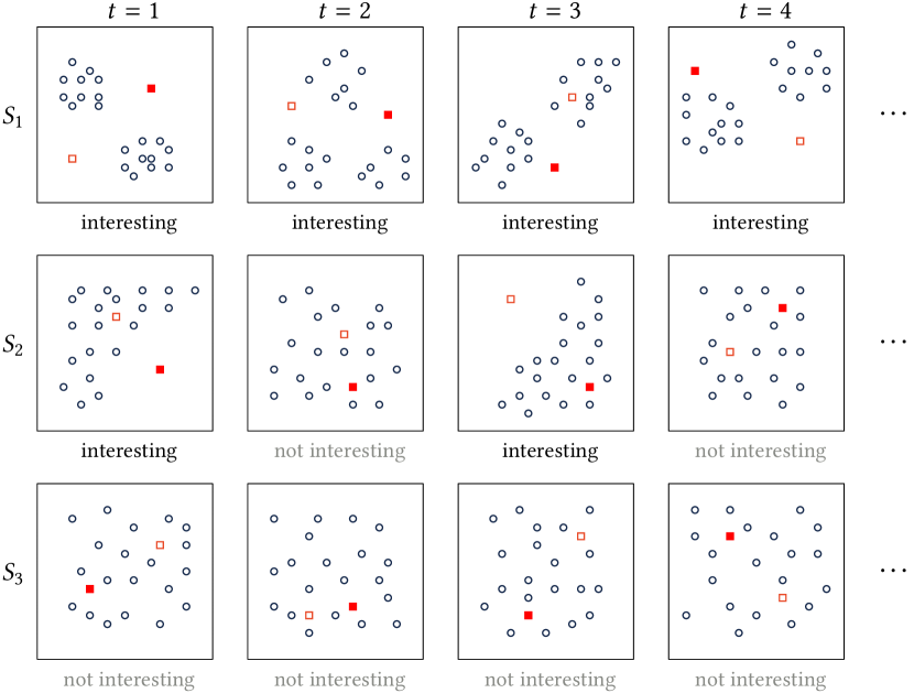
Figure 1. Subspace Search in Data Streams with outliers.

1.3. Contributions

We facilitate subspace search in data streams. After formulating the problem, we propose a new subspace search method, called Streaming Greedy Maximum Random Deviation (SGMRD).

We show that our method fulfils the above constraints. Inspired by existing static methods (Keller et al., 2012; Trittenbach and Böhm, 2019), SGMRD leverages a new multivariate dependency measure and Multi-Armed Bandit (MAB) algorithms to update the results of the search in data streams.

We perform extensive experiments, based on an assortment of synthetic and real-world data. They show that (1) our approach leads to efficient monitoring of relevant subspaces, and (2) such monitoring also improves subsequent data mining tasks, such as outlier detection. We compare our approach to competitive baselines and state-of-the-art methods.

We release our source code, experiments and documentation on GitHub, to help with the reproducibility of our study.

Outline: Section 2 covers related work, Section 3 our notation. Section 4 formulates the problem of subspace search in data streams. Section 5 presents our approach. Section 6 outlines the experimental setup. Section 7 presents our results. Section 8 concludes.

2. Related Work

Many methods for subspace search exist, but almost all of them are either coupled to a specific data mining algorithm or are limited to the static setting. For example, various approaches for streams (Kontaki et al., 2006; Zhang et al., 2007, 2008; Aggarwal, 2009) only tend to work with a given static algorithm. Other methods in turn (Keller et al., 2012; Wang et al., 2017; Bacher et al., 2016; Trittenbach and Böhm, 2019) decouple the search from the actual task, but none of them can handle streams. The existing work on subspace search mostly focuses on individual applications (Parsons et al., 2004; Kriegel et al., 2009; Zimek et al., 2012), e.g., clustering or outlier detection, while ‘general-purpose’ subspace search has received less attention.

To our knowledge, there exist two proposals to extend subspace search to streams in a general way: HCP-StreamMiner (Vanea et al., 2012) and StreamHiCS (Becker, 2016). But these approaches boil down to a periodic repetition of the procedure in (Keller et al., 2012) on synopses of the stream. We will see that our method outperforms these approaches. Greedy Maximum Deviation (GMD) (Trittenbach and Böhm, 2019) is the approach most similar to ours. It uses a so-called contrast measure (Keller et al., 2012) to quantify the interestingness of a given subspace and builds a set of subspaces via a greedy heuristic. However, GMD assumes static data.

Subspace search has been used in the past to improve the results of data mining tasks such as outlier detection (Zhang et al., 2008; Keller et al., 2012; Trittenbach and Böhm, 2019). The authors compare their results with full-space static outlier detectors. We perform an analogous evaluation in the streaming setting and compare our results against several baselines and state-of-the-art stream outlier detectors, such as xStream (Manzoor et al., 2018) and RS-Stream (Sathe and Aggarwal, 2018). See (Gupta et al., 2014) for a survey of outlier detection in streams.

3. Notation

A data stream is a set of dimensions ${D}=\{s_{1},\dots,s_{d}\}$ and an open list of observations ${B}=(\vec{{x}}_{1},\vec{{x}}_{2},\dots)$, where $\vec{{x}}_{j}$ with $j\in\mathbb{N}^{+}$ is a vector of $d$ values, and we see a dimension $s_{i}=(x_{1}^{i},x_{2}^{i},\dots)$ with $i=\{1,\dots,d\}$ as an open list of numerical values.

Since the stream is virtually infinite, we use the sliding window model: At any time ${t}\geq 1$, we only keep the ${w}$ latest observations, ${W_{t}}=\left(\vec{{x}}_{{t}-{w}+1},\dots,\vec{{x}}_{{t}}\right)$. We call a subspace ${S}$ a projection of the window ${W_{t}}$ on $|{S}|$ dimensions, with ${S}\subseteq{D}$ and $|{S}|\leq d$. $\mathcal{P}({S})$ is the power set of ${S}$, i.e., the set of all dimension subsets. We assume, without loss of generality, that observations are equidistant in time.

Window-based approaches are useful to overcome the constraints of streams, because they require a single scan of data (C2) and capture the most recent observations. Thus, algorithms based on such synopses can adapt (C3) (Gama, 2012). Note that one could easily adapt our method to accommodate other summarisation techniques, such as the landmark window or reservoir sampling (Gama, 2012).

4. Problem Formulation

4.1. Dimension-based Subspace Search

Subspace search in the static setting has already been formalised in the literature. The goal is to find a set of subspaces that fulfils a specific notion of optimality. Such subspaces must at the same time (1) be likely to reveal patterns (the ‘haystacks’ from the analogy above) and (2) be diverse, i.e., have low redundancy with each other.

To this end, the idea is to deem a set of subspaces optimal if adding or removing a subspace to/from this set makes the search results worse. To ensure diversity, the notion of optimality of each subspace must be tied to a specific dimension. This way, the resulting set may consist of the best subspaces w.r.t. each dimension, and each dimension is represented in this manner. This is the essence of what we call ‘dimension-based’ search.

To illustrate this, we show in Figure 2 an exemplary result from a dimension-based search and from another scheme. Dimension-based results are more diverse compared to other results, which tend to over-represent some dimensions. Previous work (Trittenbach and Böhm, 2019) showed that the diversity from dimension-based approaches is key to improve the performance of subspace search algorithms.

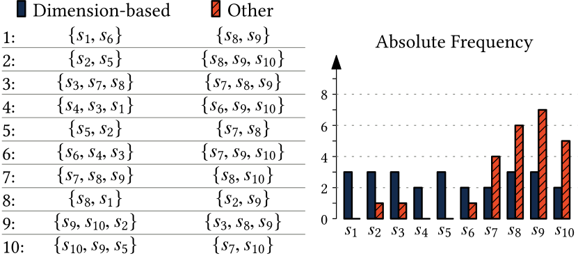
Figure 2. Dimension-based subspace search versus other methods on a toy data set ($d=10$).

Formally, we define a so-called Dimension-Subspace Quality Function (D-SQF), to capture how much a dimension $s_{i}$ helps to reveal patterns in a subspace $S$:

Definition 0 (D-SQF).

For any ${S}\in\mathcal{P}({D})$ and any ${s_{i}}\in{D}$, a Dimension-Subspace Quality Function (D-SQF) is a function of type ${q}:\mathcal{P}({D})\times{D}\mapsto[0,1]$ with $q(S,s_{i})=0,\forall{s_{i}}\notin{S}$.

$q(S,s_{i})=1$ means that $S$ has the maximum potential to reveal patterns w.r.t. $s_{i}$. Put differently, patterns may become more visible as one includes $s_{i}$ in $S$. This measure is asymmetric. For example, the quality of subspace $\{s_{1},s_{2}\}$ does not need to be the same w.r.t. $s_{1}$ or $s_{2}$. In turn, $q(S,s_{i})=0$ means that $S$ cannot reveal any patterns w.r.t. $s_{i}$. By definition, $q(S,s_{i})=0$ if ${s_{i}}$ is not part of ${S}$ because the subspace cannot reveal any pattern in ${s_{i}}$.

Recent studies (Wang et al., 2017; Trittenbach and Böhm, 2019) instantiate such D-SQF as a measure of correlation, which one can estimate without any ex-post evaluation, i.e., it is not specific to any data mining algorithm. With this, subspace search remains independent of any downstream task. We can define a notion of subspace optimality:

Definition 0 (Optimal Subspace).

A subspace ${S}\in\mathcal{P}({D})$ is optimal w.r.t. ${s_{i}}\in{D}$ and a D-SQF $q$ if and only if

$${q}({S},{s_{i}})\geq{q}(S^{\prime},{s_{i}})\quad\forall S^{\prime}\in\mathcal{P}({D}).$$

Then the optimal subspace set $\mathbb{S}^{*}$ is the set of optimal subspaces in $D$ w.r.t. each dimension $s_{i}\in D$:

Definition 0 (Optimal Subspace Set).

A set $\mathbb{S}^{*}$ is optimal w.r.t. $D$ and a D-SQF ${q}$ if and only if

$$\forall s_{i}\in D,\leavevmode\nobreak\ \exists S\in\mathbb{S}^{*}\leavevmode\nobreak\ s.t.\leavevmode\nobreak\ \forall S^{\prime}\in\mathcal{P}(D),\leavevmode\nobreak\ q(S,s_{i})\geq q(S^{\prime},s_{i}).$$

Thus, the optimal set $\mathbb{S}^{*}$ contains one subspace $S$ for each dimension ${s_{i}}\in{D}$, each one maximising the quality ${q}$ w.r.t. ${s_{i}}$. I.e., we can see $\mathbb{S}^{*}$ as a mapping of each dimension ${s_{i}}\in{D}$ to an optimal subspace w.r.t. that dimension:

$$\mathbb{S}^{*}:{s_{i}}\in{D}\mapsto{S}\in\mathcal{P}({D})\quad s.t.\quad\forall S^{\prime}\in\mathcal{P}({D})\quad{q}({S},s_{i})\geq{q}(S^{\prime},s_{i}).$$

Finding $\mathbb{S}^{*}$ is NP-hard (Nguyen, 2015). This is because one needs to assess the D-SQF of a set whose size grows exponentially with the number of dimensions. In fact, even finding a single optimal subspace is NP-hard. Thus, existing techniques do not guarantee the optimality of the results, but instead target at a good approximation of $\mathbb{S}^{*}$, while keeping the number of subspaces considered small.

This idea is suitable in the static setting (Keller et al., 2012; Wang et al., 2017). (Trittenbach and Böhm, 2019) showed that it leads to diverse sets of subspaces with better downstream mining results. Here, we propose a generalisation for streams.

4.2. Subspace Search in the Streaming Setting

The quality of subspaces, estimated via statistical correlation measures, may change over time, manifesting a phenomenon known as ‘concept drift’ (Barddal et al., 2015). Thus, in streams, the quality function $q$ is time-dependent, and so we write $\mathbb{S}_{t}^{*}$ and ${q_{t}}$. Then the problem becomes more complex — observe the following example:

Example 4.4 (Variation of Mutual Information).

We obtained measurement data from a power plant and computed the evolution of correlation (estimated via Mutual Information) between a set of 10 sensor pairs for a single day. Figure 3 graphs the results. The Mutual Information for pairs $1$ and $2$ remains stable for the whole duration, while it is more volatile for pairs $3$ to $6$. The pairs $7$ to $10$ in turn show some change, but with less variance.

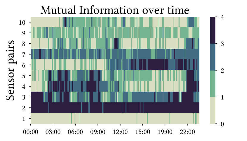
Figure 3. Evolution of Mutual Information between 10 sensor pairs in an experimental power plant for one day of data.

As the example shows, some subspaces remain optimal for a longer period of time, while others frequently become sub-optimal. So the difficulty is that, even if one finds the set of subspaces $\mathbb{S}_{t}^{*}$, there is no guarantee that this set is optimal at time ${t}+1$. Next, it is impossible to even test the optimality of $\mathbb{S}_{t}^{*}$, because one would need to evaluate an exponential number of subspaces.

Let us assume that the cost of evaluating the quality of a subspace is constant across different subspaces and time. This is the case when considering existing correlation estimators. We define a function $\mathcal{E}_{t}:\mathcal{P}(D)\times D\mapsto\{0,1\}$ such that $\mathcal{E}_{t}(S,s_{i})=1$ if a given search scheme computes $q_{t}(S,s_{i})$, else $0$. We can now formulate subspace search in data streams as a multi-objective optimisation problem at time ${t}$ with two conflicting objectives:

1. Find a set $\mathbb{S}_{t}$ which approximates $\mathbb{S}_{t}^{*}$ well. I.e., minimise an objective $O_{1}=\sum_{i=1}^{d}\left[q_{t}(\mathbb{S}_{t}^{*}({s_{i}}),s_{i})-q_{t}(\mathbb{S}_{t}({s_{i}}),s_{i})\right]$; the sum of the differences between the quality of the optimal set and the quality of the approximate set for each dimension.

2. Reduce the computation of the search, i.e., minimise an objective $O_{2}=\sum_{{s_{i}}}^{{D}}\sum_{{S}}^{\mathcal{P}({D})}\mathcal{E}_{t}(S,s_{i})$; the number of subspaces for which one computes the quality at time $t$.

If $O_{1}=0$, then $\mathbb{S}_{t}\equiv\mathbb{S}_{t}^{*}$. Conversely, if $O_{2}=0$, then choosing $\mathbb{S}_{t}$ boils down to random guessing. Thus, $O_{1}$ and $O_{2}$ conflict. They capture the trade-off between the quality of the set of subspaces and the computation effort.

Definition 4.3 implies that the search is independent for each dimension. Thus, to optimise $O_{1}$, we must find a dimension-based search algorithm, which for any dimension $s_{i}\in D$, returns a near-optimal subspace $S$ w.r.t. the dimension. More formally:

Definition 0 (Dimension-based Search Algorithm).

A search algorithm, that is dimension-based, is a function $\mathit{Search}_{t}:D\mapsto\mathcal{P}(D)$, which for any dimension $s_{i}\in D$, returns a subspace $S$ minimising $q_{t}(\mathbb{S}_{t}^{*}(s_{i}),s_{i})-q_{t}(S,s_{i})$ at time $t$.

Such an algorithm is associated with a cost, which depends on the number of subspaces evaluated. I.e., each run of $\mathit{Search}_{t}$ negatively impacts objective $O_{2}$. Thus, an additional challenge is to find an update policy $\pi:t\mapsto\mathcal{P}(D)$ to decide at any time for which dimension(s) one should repeat the search. We define it as follows:

Definition 0 (Update Policy).

An update policy is a function $\pi:t\mapsto\mathcal{P}(D)$.

The policy returns for any time $t$ a set of dimensions $I_{t}\in\mathcal{P}(D)$, so that one repeats the $\mathit{Search}_{t}$ algorithm for $s_{i}\in I_{t}$.

Overall, to achieve subspace search in data streams, we must come up with an adequate instantiation of the following elements:

• A D-SQF $q_{t}:\mathcal{P}({D})\times{D}\mapsto[0,1]$.

• A dimension-based search algorithm $\mathit{Search}_{t}:D\mapsto\mathcal{P}(D)$.

• An update policy $\pi:t\mapsto\mathcal{P}(D)$.

Our approach, Streaming Greedy Maximum Random Deviation (SGMRD), addresses the challenges described previously by instantiating and combining each of these elements in a general framework.

5. Subspace Search in Data Streams

Figure 4. SGMRD: A High-Level Overview. At any time, SGMRD delivers a set of high-quality subspaces $S_{1},\dots,S_{d}$.

5.1. Our Approach: SGMRD

Figure 4 shows an overview of our framework, in two steps:

1. Initialisation. We find an initial set of subspaces $\mathbb{S}_{0}$, using the first ${w}$ observations in the stream. To do so, we run the algorithm $\mathit{Search}_{t}$ for each dimension. The outcome of this step is a set of subspaces $S_{1},\dots,S_{d}$, one for each dimension.

2. Maintenance. For any new observation in the stream, we monitor the quality of subspaces $q_{t}(S,s_{i})$ for $S\in\mathbb{S}_{t}$, and decide, by learning a policy $\pi$, for which dimension(s) we repeat the search, i.e., algorithm $\mathit{Search}_{t}$.

Our approach is general to some extent, as one could consider various instantiations of each building block (Search, Monitor and Update). With SGMRD, we instantiate the search function $\mathit{Search}_{t}$ as a greedy hill-climbing heuristic, $q_{t}$ as an efficient dependency estimator and the policy $\pi$ as a Multi-Armed Bandit (MAB) algorithm with multiple plays. We describe the specifics of each block and explain our design decisions in the following sections.

5.1.1. Search

SGMRD’s initialisation searches for an initial set of subspaces using the first observation window. Since finding the optimal set (cf. Definition 4.3) is not feasible, we instantiate $\mathit{Search}_{t}$ as a greedy hill-climbing heuristic. Our heuristic constructs subspaces in a bottom-up, greedy manner. Algorithm 1 is our pseudo-code, and Figure 5 illustrates our idea with a toy example.

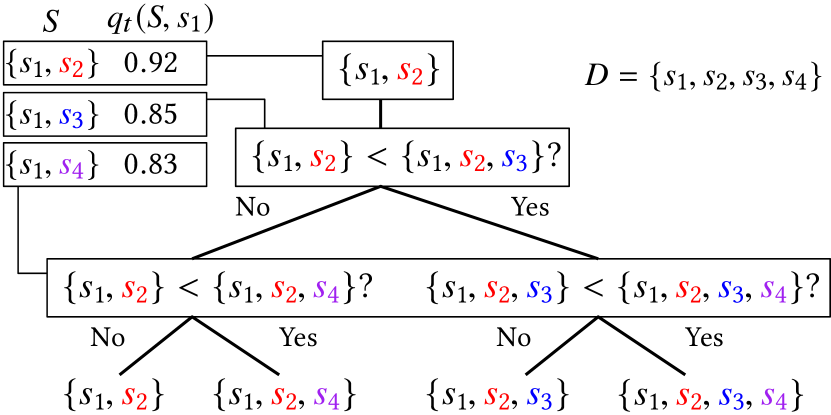
Figure 5. Example of search w.r.t. $s_{1}$ with four dimensions.

In a first step (Line 2), we select the 2-dimensional subspace maximising the quality w.r.t. $s_{i}$. In our example, $s_{i}=s_{1}$, and the subspace with the highest quality is $\{s_{1},s_{2}\}$. Then we iteratively test whether adding the dimension associated with the next best 2-dimensional subspace containing $s_{i}$ (Line 5) increases the quality of the current subspace (Line 6). If this is the case, we add it into the current subspace (Line 7), otherwise, we discard it. In our example, the heuristic first considers adding $s_{3}$, then $s_{4}$.

The advantage of only considering 2-dimensional subspaces for selecting the next dimension is that it keeps the runtime of the search linear w.r.t. the number of dimensions. More precisely, we can see that the heuristic computes the quality of exactly $(d-1)+(d-2)=2d-3$ subspaces. Thus, the runtime of Algorithm 1 is in $O(d)$. The search is independent for each dimension. At initialisation, we run it for each dimension, so the initialisation is in $O(d^{2})$.

Algorithm 1 $\mathit{Search}_{t}$(${s_{i}}$)

1:A dimension ${s_{i}}\in{D}$

2:$\mathcal{S}^{\mathit{max}}\leftarrow{s_{i}}\cup\left(\operatorname*{arg\,max}_{s_{j}\in{S}}q_{t}({s_{i}}\cup s_{j},{s_{i}})\right)$

3:${S}\leftarrow{S}\setminus\mathcal{S}^{\mathit{max}}$

4:while  ${S}$ is not empty do

5:    $\mathcal{S}^{\mathit{cand}}\leftarrow\operatorname*{arg\,max}_{s_{j}\in{S}}q_{t}({s_{i}}\cup s_{j},{s_{i}})$

6:    if $q_{t}(\mathcal{S}^{\mathit{max}}\cup\mathcal{S}^{\mathit{cand}},{s_{i}})>q_{t}(\mathcal{S}^{\mathit{max}},{s_{i}})$ then

7:         $\mathcal{S}^{\mathit{max}}\leftarrow\mathcal{S}^{\mathit{max}}\cup\mathcal{S}^{\mathit{cand}}$     

8:    ${S}\leftarrow{S}\setminus\mathcal{S}^{\mathit{cand}}$

9:return subspace $\mathcal{S}^{\mathit{max}}\subseteq{D}$

5.1.2. Monitor

So far, we did not discuss any concrete instantiation of the quality $q_{t}$. In practice, one has only a sample of observations, and thus, the quality can only be estimated from a limited number of points. In what follows, we describe a new method to estimate the quality. Considering the constraints from the streaming setting (cf. Section 1.2) and the nature of the required quality function, our method must fulfil the following technical requirements:

Efficiency. Since the search includes estimating the quality of numerous subspaces, the quality-estimation procedure must be efficient, to cope with the streaming constraints (C1).

Multivariate. Since subspaces can have an arbitrary number of dimensions, the quality measure must be multivariate. Traditional dependency estimators in turn are bivariate (Joe, 1989).

Asymmetric. Since the quality values are specific for a given dimension, the measure is not symmetric.

We define the quality as a measure of non-independence in subspace $S$ w.r.t. $s_{i}$. Observe the following definition of independence:

Definition 0 (Independence of Random Variables).

A random vector $X=\{X_{1},\dots,X_{n}\}$ is independent if and only if $p_{X}=\prod_{i=1}^{n}p_{X_{i}}$, where $p_{X}$ is the joint distribution and $p_{X_{1}},\dots,p_{X_{n}}$ are the marginal distributions.

This implies that the marginal distributions of each variable $X_{i}$ must be equal to their conditional distribution w.r.t. $X\setminus X_{i}$. By seeing each dimension as a random variable, we can estimate the quality as a degree of non-independence w.r.t. a dimension $X_{i}$, and quantify it as the discrepancy between the empirical marginal distribution $\hat{p}_{X_{i}}$ and the conditional distribution $\hat{p}_{X_{i}|(X\setminus X_{i})}$.

For the ease of discussion, let us consider $q_{t}(\{s_{1},s_{2}\},s_{1})$. Then,

(1) $$q_{t}(\{s_{1},s_{2}\},s_{1})\propto disc\left(\hat{p}_{s_{1}},\hat{p}_{s_{1}|s_{2}}\right),$$

where $disc$ is the discrepancy between both distributions.

To estimate this discrepancy, we propose a bootstrap method. Iteratively, we take a random condition w.r.t. the dimensions $S\setminus s_{1}$ (i.e., restricting the other dimensions to a random interval) and perform a statistical test between the sets of observations within and outside of this random condition w.r.t. $s_{1}$.

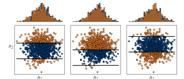
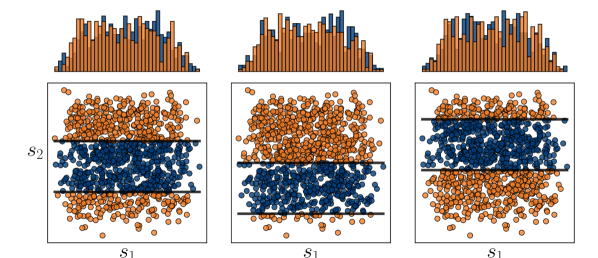
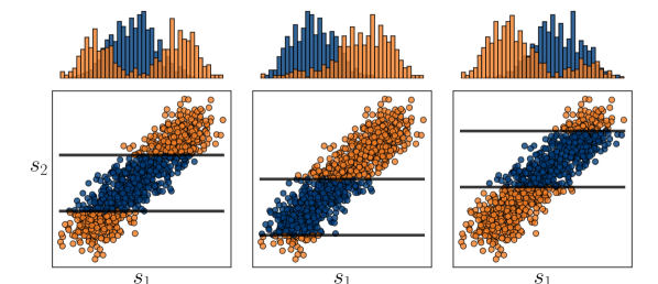
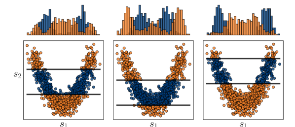
Figure 6. Our approach to estimate subspace quality.

Figure 6 illustrates this idea with two subspaces showing an independent 2-dimensional distribution and two subspaces with a linear and quadratic dependence. As we can see, over three randomly chosen conditions, the distributions of both sets of observations (see the histograms) are very similar for the first two subspaces, while they are markedly different for the other ones. Intuitively, subspaces with dependence are more likely to reveal patterns such as clusters or outliers, which are not visible in any other subspace.

To estimate $q_{t}$, we average the discrepancies over $M$ iterations:

(2) $$q_{t}(S,s_{i})=1-\frac{1}{M}\sum_{j=1}^{M}\mathcal{T}\left(\hat{p}_{S|c_{j}(s_{i})},\hat{p}_{S|\overline{c_{j}}(s_{i})}\right),$$

where $c_{j}(s_{i})$ is a random condition w.r.t. $s_{i}$, and the $\overline{c_{j}}(s_{i})$ is its complementary condition in the current window of data. The resulting two sets of observations respectively are in dark blue and light orange in the figure. $\mathcal{T}$ yields the p-value of a two-sample Kolmogorov-Smirnov test. This test is adequate as it has high power and it is non-parametric. However, other tests are possible as well, see (Siegel and Castellan, 1988). In the end, $q_{t}(S,s_{i})$ converges to $1$ as the evidence against independence between both conditional distributions increases. It is efficient, because testing requires only linear time, while conditioning requires a one-time sorting of the elements in the window.

Our examples in Figure 6 are limited to two dimensions for the sake of illustration. However, one can easily extend this principle to multiple dimensions, as in (Keller et al., 2012). Based on Hoeffding’s inequality (Hoeffding, 1963), it is easy to show that our measure converges to its expected value as the number of iterations $M$ increases, formally:

(3) $$\Pr\left(|q_{t}(S,s_{i})-\mathbb{E}(q_{t}(S,s_{i}))|\geq\varepsilon\right)\leq 2e^{-2M\varepsilon^{2}}.$$

See (Fouché and Böhm, 2019; Fouché et al., 2020) for the corresponding proof. This brings several advantages: We can estimate the quality in quasi-linear time w.r.t. the number of points and reduce the number of iterations $M$ to adapt to the speed of streams. Thus, the approach is anytime (C4).

To monitor the quality estimates of each subspace in $\mathbb{S}_{t}$ over time, we smooth out the statistical fluctuations of the estimation process via exponential smoothing with parameter $\gamma$. Preliminary experiments showed that $M=100$ with $\gamma=0.9$ leads to good estimation quality and performance w.r.t. downstream tasks. The outcome is a smoothed quality function $Q_{t}:{D}\mapsto[0,1]$:

(4) $$Q_{t+1}({s_{i}})=\gamma\cdot q_{t}(\mathbb{S}_{t}(s_{i}),{s_{i}})+(1-\gamma)\cdot{q}_{{t}+1}(\mathbb{S}_{t}(s_{i}),{s_{i}}).$$

5.1.3. Update

The initialisation step is relatively expensive, because one needs to run the search (Algorithm 1) for each dimension.

While running the search for every dimension optimises the quality of the subspace set (Objective $O_{1}$), it curbs efficiency (Objective $O_{2}$). However, as in Example 4.4, the dependence between dimensions can unexpectedly change over time. Thus, without any assumption, it is not possible to exploit our knowledge from step $t-1$. We mitigate the computational cost over time by only repeating the search for a few dimensions at each time step.

The challenge is to find a policy $\pi:t\mapsto\mathcal{P}(D)$ to decide at any time step $t$ for which $L$ dimensions to repeat the search, where $L<d$ is a budget per time step. The budget $L$ can either be set by the user, or it is based on the computational time available between two subsequent observations.

To solve this challenge, we cast the decisions of the policy $\pi$ as a MAB problem with multiple plays (Komiyama et al., 2015). Multi-Armed Bandit (MAB) models are useful tools to capture the trade-offs of sequential decision making problems. In what follows, we use the common notation from the bandit literature, as in (Bubeck and Cesa-Bianchi, 2012). We model each dimension $s_{i}\in D$ as an ‘arm’. In each round $t=\{1,\dots,T\}$, the policy $\pi$ selects $L<d$ arms $I_{t}\subset D$ and runs the search for each $s_{i}\in I_{t}$. Then there are two possible outcomes for each $s_{i}$:

1. Success: $\mathit{Search}_{t}(s_{i})$ yields a better subspace than $\mathbb{S}_{t-1}(s_{i})$, so we update $\mathbb{S}_{t}({s_{i}})$. The policy receives a reward of $1$.

2. Failure: $\mathit{Search}_{t}(s_{i})$ does not yield a better subspace, so we set $\mathbb{S}_{t}({s_{i}})\leftarrow\mathbb{S}_{{{t}}-1}({s_{i}})$. The reward is $0$.

Since the rewards are binary, we can associate each arm $s_{i}\in D$ with a Bernoulli distribution with unknown mean $\mu_{i}$. The goal of a multiple-play MAB algorithm is to find the top-$L$ arms with largest reward expectation $\mu_{i}$ from empirical observations with as few trials as possible (Komiyama et al., 2015). In our case, this means finding the $L$ dimensions for which one must repeat the search more frequently.

To find the best arms, we employ an algorithm known as Multiple-Play Thompson Sampling (MP-TS) (Komiyama et al., 2015). In a nutshell, Thompson Sampling is a Bayesian inference heuristic which selects an arm based on posterior samples of the expectations of each arm. Since the Beta distribution is a conjugate prior for the Bernoulli distribution, $\mathit{Beta}(\alpha_{i},\beta_{i})$ is the prior belief for arm $i$, and for each arm $i$, we maintain a pair of parameters $\alpha_{i},\beta_{i}$. At each step, we sample from each $\mathit{Beta}(\alpha_{i},\beta_{i})$ distribution and play the arms with highest value. Whenever we observe a success after playing arm $i$, we increment $\alpha_{i}$, otherwise we increment $\beta_{i}$. Assuming a uniform initial prior, we initialise $\alpha_{i},\beta_{i}=1$. The idea of Thompson Sampling traces back to 1933 (Thompson, 1933), but recent studies demonstrate its superiority over other bandits in theory and practice (Kaufmann et al., 2012; Chapelle and Li, 2011).

Intuitively, the behaviour of the policy $\pi$ is to explore in the beginning, by playing various arms, and then to exploit the high-reward arms, i.e., repeating the search for dimensions whose optimal subspace changes more frequently. Algorithm 2 is the pseudo-code for our update step.

Algorithm 2 $\mathit{Update}_{t}$($\mathbb{S}_{t}$, $L$)

1:A set of subspaces $\mathbb{S}_{t}$, the number of plays per round ${L}$.

2:for $i=1,\dots,{K}$ do

3:    $\theta_{i}(t)\sim\mathit{Beta}(\alpha_{i}(t),\beta_{i}(t))$

4:${I_{t}}=\operatorname*{arg\,max}_{K^{\prime}\subset[{K}],|K^{\prime}|={L}}\sum_{i}^{K^{\prime}}\theta_{i}(t)$

5:for $i\in{I_{t}}$ do

6:    $S\leftarrow\mathit{Search}_{t}({s_{i}})$ $\triangleright$ Searching for a new subspace w.r.t. $s_{i}$

7:    if ${q}_{{t}+1}({S},{s_{i}})>Q_{t+1}(\mathbb{S}_{t}({s_{i}}),{s_{i}})$ and ${S}\neq\mathbb{S}_{t}({s_{i}})$ then

8:         $\mathbb{S}_{{{t}}+1}({s_{i}})\leftarrow{S}$ ; $\alpha_{i}(t+1)=\alpha_{i}(t)+1$

9:    else

10:         $\mathbb{S}_{{{t}}+1}({s_{i}})\leftarrow\mathbb{S}_{t}({s_{i}})$ ; $\beta_{i}(t+1)=\beta_{i}(t)+1$     

11:return $\mathbb{S}_{{{t}}+1}$

Algorithm 3 SGMRD((${D},{B}$), ${w}$, $L$, $\gamma$)

1:Data stream (${D},{B}$), window size $\mathit{{w}}>0$, $L>0$, $\gamma\in(0,1)$

2:${t}\leftarrow{w}$ $\triangleright$ 1. Initialisation

3:for $s_{i}\in D$ do

4:    $\mathbb{S}_{t}(s_{i})\leftarrow\mathit{Search}_{t}({s_{i}})$ $\triangleright$ Search

5:while ${B}$ has a new observation $\vec{{x}}_{{{t}}+1}$ do $\triangleright$ 2. Maintenance

6:    ${t}\leftarrow{t}+1$

7:    for $s_{i}\in D$ do $\triangleright$ Monitor

8:         $Q_{t}({s_{i}})=\gamma\cdot q_{t-1}(\mathbb{S}_{t-1}(s_{i}),{s_{i}})+(1-\gamma)\cdot{q}_{{t}}(\mathbb{S}_{t}(s_{i}),{s_{i}})$     

9:    $\mathbb{S}_{t}\leftarrow\mathit{Update}_{t}(\mathbb{S}_{{{t}}-1},L)$ $\triangleright$ Update

10:return at anytime the set of subspaces $\mathbb{S}_{t}$

5.1.4. SGMRD

Algorithm 3 summarises our approach as pseudo-code. SGMRD finds an initial set of subspaces using the first window (Line 4). Then SGMRD monitors and updates the set of subspaces (Line 7 to 9) for each new observation $\vec{x}_{t+1}$.

Overall, our method, SGMRD, is efficient (C1), as our quality estimates can be computed in linear time. It also requires a single scan of the data (C2), as we monitor subspaces over a sliding window. By design, SGMRD adapts (C3) to the environment by updating the subspace search results with parsimonious resource consumption, and our experiments will confirm this. Finally, results are available at any point in time (C4).

In addition to reducing the number of plays ${L}$, one can further bring down the computational requirements of SGMRD by performing the update step (Line 9) only once every $v$ new observations. For simplicity, we have described Algorithm 3 with $v=1$.

In our experiments, we will study the trade-off between the quality of the results and the cost associated with our method.

5.2. Downstream Data Mining

High-quality subspaces can be useful for virtually any downstream data mining task. For example, previous work (Keller et al., 2012; Nguyen et al., 2016b; Wang et al., 2017; Trittenbach and Böhm, 2019) leverages subspaces to build ensemble-like outlier detectors. Other data mining tasks are possible as well, such as clustering (Park and Lee, 2007; Zhang et al., 2007; Agrawal et al., 2005; Aggarwal, 2009; Kontaki et al., 2006). Our approach, SGMRD, yields a set of subspaces $\mathbb{S}_{t}$ at any time. While our approach is not tied to any specific data mining task, we use outlier detection as an exemplary task in our evaluation.

The articles just cited apply an outlier detector to each subspace in $\mathbb{S}_{t}$, and the final score is a combination of the individual scores. The outcome is a ranking of objects by decreasing ‘outlierness’. In the experiments that follow, we use the LOF detector because it is a common baseline in the outlier detection literature (Keller et al., 2012).

The best combination of the individual scores depends on the concrete application. Literature has discussed this extensively (Aggarwal and Sathe, 2015; Nguyen et al., 2016a). Several studies (Lazarevic and Kumar, 2005; Pokrajac et al., 2007) argue that the average of the scores with LOF yields the best results overall in the static case, so we stick to this choice. The final outlier score of $\vec{{x}}_{{t}}$ is the average of the scores from each subspace across every window containing $\vec{{x}}_{{t}}$:

(5) $$\textit{score}^{\leavevmode\nobreak\ }(\vec{{x}}_{{t}})=\frac{1}{{w}\cdot d}\sum_{i=0}^{{w}}\sum_{{s_{i}}}^{\mathbb{S}_{{{t}}-i}}score_{W_{{{t}}-i}}^{\mathbb{S}_{{{t}}-i}({s_{i}})}(\vec{{x}}_{{t}}).$$

Again, one may also reduce the computation effort of outlier detection by evaluating the scores only once every $v$ time steps.

6. Experiment Setup

We evaluate the performance of our approach w.r.t. two aspects: (1) the quality of subspace monitoring, i.e., how efficiently and effectively can SGMRD maintain a set of high-quality subspaces over time, and (2) the benefits w.r.t. outlier detection, as an exemplary downstream data mining task.

6.1. Evaluation Measures

6.1.1. Subspace Monitoring

Evaluating the quality of subspace monitoring is difficult because finding $\mathbb{S}_{t}^{*}$ is computationally infeasible for non-trivial data. Thus, based on the definition of objective $O_{1}$ (cf. Section 4.2), we measure the regret and the average quality:

(6) $$R_{{T}}=\frac{1}{d}\sum_{{t}=0}^{{{T}}}\sum_{{i}=1}^{d}\left[{Q}_{{t}}^{*}(s_{i})-Q_{{t}}(s_{i})\right],\leavevmode\nobreak\ \overline{Q}_{{t}}=\frac{1}{d}\sum_{{i}=1}^{d}Q_{{t}}(s_{i}),$$

where $Q_{{t}}(s_{i})$ is the quality w.r.t. $s_{i}$ as defined in Equation 4, and ${Q}_{{t}}^{*}(s_{i})$ is the quality obtained when one always updates the corresponding subspace, i.e., it the same as repeating the initialisation. $R_{{T}}$ is the regret, defined as the sum of the differences between ${Q}_{{t}}^{*}(s_{i})$ and $Q_{{t}}(s_{i})$ up to time $T$. $\overline{Q}_{{t}}$ is the average quality at time $t$, and $\overline{Q}_{{T}}$ is the average quality up to time $T$.

To characterise the behaviour of our update strategy, we also look at the relative update frequency $F_{{T}}({s_{i}})$ for each dimension ${s_{i}}\in{D}$ and the rate of successful updates $U_{{T}}$, as in Section 5.1.3, i.e.:

(7) $$F_{{T}}({s_{i}})=\sum_{{t}=0}^{{{T}}}\frac{\mathbf{1}\left[{s_{i}}\in{I_{t}}\right]}{T},\leavevmode\nobreak\ U_{{T}}=\sum_{{t}=0}^{{{T}}}\sum_{{i=1}}^{{d}}\frac{\mathbf{1}\left[A_{t}(s_{i})\wedge B_{t}(s_{i})\right]}{d\cdot{{T}}},$$

where ${s_{i}}\in{I_{t}}$ means that SGMRD has selected dimension ${s_{i}}$ at time ${t}$, and $A_{t}(s_{i})$ and $B_{t}(s_{i})$ are the conditions capturing whether the search was successful (i.e., the new subspace is different and of higher quality than the previous one):

(8) $$A_{t}(s_{i}) =\mathbb{S}_{{{t}}-1}({s_{i}})\neq\mathbb{S}_{t}({s_{i}}),$$

(9) $$B_{t}(s_{i}) =Q_{t}(\mathbb{S}_{{{t}}-1}({s_{i}}),{s_{i}})<q_{t}(\mathbb{S}_{t}({s_{i}}),{s_{i}}).$$

6.1.2. Outlier Detection

By definition, outliers are rare, so the detection of outliers is an imbalanced classification problem. We report the area under the ROC curve (AUC) and the Average Precision (AP), which are popular measures for evaluating outlier detection algorithms. Outlier detectors typically ranks the observation by decreasing ‘outlierness’, measured as a score. In most applications, end users only check the top X% items. So we report the Recall (R) and Precision (P) within the top X% instances, with $\text{X}\in\{1,2,5\}$.

6.2. Data Sets

We use an assortment of data sets for our evaluation. One is a data set from a real-world use case, corresponding to measurements in a pyrolysis plant. We also include four real-world data sets with outlier ground truth: KDDCup99, Activity, Backblaze, Credit. While the former two have frequently been used in the literature, the latter two are our own addition to this benchmark. To cope with the lack of publicly available data sets for outlier detection in the streaming setting, we also generate three synthetic benchmark data sets: Synth10, Synth20 and Synth50. We describe each data set in detail hereafter; Table 1 summarises their main characteristics.

Table 1. Characteristics of the Benchmark Data Sets.

Benchmark	# Instances	# Dimensions	% Outliers
Pyro	$10000$	100	NA
KDDCup99	$25000$	38	7.12
Activity	$22253$	51	10
Backblaze	$12600$	44	1
Credit	$284807$	29	0.17
Synth10	$10000$	10	0.86
Synth20	$10000$	20	0.88
Synth50	$10000$	50	0.81

6.2.1. Real-World Data Sets

• Pyro: This data set contains $10000$ measurements (one per second) from a selection of 100 sensors, such as temperature or pressure, in various components of a pyrolysis plant. We use this data set to evaluate how well our method can search for subspaces in data streams. However, there is no ground truth, so we cannot use this data set for our downstream data mining application.

• Activity: This data set, initially proposed in (Reiss and Stricker, 2012), describes different subjects performing various activities (e.g., walking, running), monitored via body-mounted sensors. Analogously to (Sathe and Aggarwal, 2018), we took the walking data of a single subject and replaced 10% of the data with nordic walking data, which we marked as outliers. The rest of the elements are inliers. We obtained the original data set from (Dua and Graff, 2017).

• KDDCup99: This data set was part of the KDD Cup Challenge 1999. It is a network intrusion data set. Analogously to (Sathe and Aggarwal, 2018), we excluded DDoS (Denial-of-Service) attacks and marked all other attacks as outliers. We take a contiguous subset of $25000$ data points. We obtained this data set from (Dua and Graff, 2017).

• Backblaze: Similarly as in (C. et al., 2017), we obtained hard drive failure stats data from Backblaze, a computer backup and cloud storage service. We prepare a benchmark with the data from Q1 2020. We select the hard drive model ST12000NM0007, because of its relatively high failure rate, and downsample the instances from the normal class such that the outliers represent $1\%$ of the total observations.

• Credit: This data set was released via the ‘credit card fraud detection’ challenge (Pozzolo et al., 2018). It is highly imbalanced, with only $0.17\%$ outliers. Also, it has comparably more instances.

6.2.2. Synthetic Benchmark Generation

In addition, we create three data sets simulating concept drift (Barddal et al., 2015) via random variations of the data distribution over time. We generate $n+1$ distributions $\Gamma_{0},\Gamma_{1},\dots,\Gamma_{n}$, and sample from each distribution $\Gamma_{i}$ a number $e$ of observations, while letting the distribution $\Gamma_{i}$ gradually drift towards the distribution $\Gamma_{i+1}$ as we sample from it.

We initialise $\Gamma_{0}\equiv\mathcal{U}[0,1]$ over the full space $D$. Then we select a set of distinct subspaces (i.e., the subspaces do not have any dimension in common) from $\mathcal{P}({D})$ for each other distribution, so that $50\%$ of the subspaces change from one distribution to the next one. For each subspace and, with a small probability $p\in(0,1)$, we sample the next point from $\mathcal{U}[\delta,1]$ for each dimension with $\delta\in(0,1)$ chosen randomly. We call this point an ‘outlier’. With probability $1-p$, we sample the next point uniformly from the rest of the unit hypercube – this is an ‘inlier’. Figure 7 illustrates this principle with two dimensions. For the dimensions not part of any subspace, every observations are i.i.d. in $\mathcal{U}[0,1]$.

Outliers placed this way are said to be ‘non-trivial’ (Keller et al., 2012), since they do not appear in any other subspace — they are ‘hidden’ in the data. Our goal is to evaluate to what extent different approaches can detect such outliers.

We generate three benchmark data sets with $n=10$ distributions and $e=1000$ observations. We set $p<0.01$, since outliers are rare by definition. Synth10, Synth20, Synth50 have $10$, $20$ and $50$ dimensions respectively, with subspaces up to $5$ dimensions.

Note that we release the code for our data generator and our real-world benchmark data sets via our GitHub repository as well.

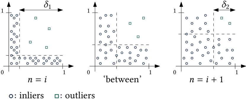
Figure 7. The synthetic benchmark generation process.

6.3. Baselines and Competitors

6.3.1. Subspace Monitoring

Our goal is to assess how effectively SGMRD can handle the trade-off between computational cost and monitoring quality. We compare SGMRD to several alternative update strategies and against several baselines.

• SGMRD-TS uses MP-TS (cf. Section 5.1.3) as update strategy, and we set $L=1$, unless noted otherwise.

• SGMRD-RD uses a random (RD) update strategy. We update a single subspace per time step, chosen at random from the current set.

• SGMRD-GD uses a greedy (GD) update strategy. We update a single subspace per time step and choose the subspace with the lowest quality.

• Batch repeats the initialisation of SGMRD periodically for every batch of data with size ${w}=1000$.

• Init runs the initialisation and then keeps the same set of subspaces for the rest of the experiment (no update).

• Gold repeats the initialisation of SGMRD at every step. This baseline represents the highest level of quality that one can reach with this instantiation of SGMRD, but it also is the most expensive configuration. In fact, we can only afford to run it on the Pyro data set.

6.3.2. Outlier Detection

We compare the results from SGMRD-TS with the following detectors:

• RS-Stream is an adaptation of the RS-Hash (Sathe and Aggarwal, 2016) outlier detector to the streaming setting, presented in (Sathe and Aggarwal, 2018). It estimates the outlierness of each observation via randomised hashing over random projections. We reproduce the approach and use the default parameters recommended by the authors.

• LOF (Breunig et al., 2000) is a well-known outlier detector. We run it periodically and average the scores over a sliding window. We use the implementation from ELKI (Schubert et al., 2015), which profits from efficient index structures.

• xStream (Manzoor et al., 2018) is an ensemble outlier detector. xStream estimates densities via randomised ensemble binning from a set of random projections. xStream declares the points lying in low density areas as outliers. We use the reference implementation with the recommended parameters.

• StreamHiCS (Becker, 2016) is an adaptation of (Keller et al., 2012), repeating the initial search, based on the signals from a change detector on a data synopsis. We use the reference implementation with the recommended parameters.

We average the scores obtained from each detector over a sliding window of size $w=1000$ for every $v=100$ time steps (cf. Section 5.2). For approaches based on LOF, such as ours, we repeat the computation with parameter $k\in\{1,2,5,10,20,50,100\}$ and report the best result in terms of AUC. The performance may vary widely w.r.t. this parameter; this is a well-known caveat of LOF (Campos et al., 2016). We average every result from $10$ independent runs. Each approach runs single-threaded on a server with 20 cores at 2.2GHz and 64GB RAM. We implement our algorithms in Scala.

7. Results

7.1. Subspace Monitoring

We first evaluate the quality of monitoring from SGMRD. We set ${w}=1000$, $v=2$ and ${L}=1$, i.e., for each update strategy, SGMRD only keeps the latest $1000$ observations, and, for any new two observations, SGMRD attempts to replace one of the current subspaces.

As we can see in Figure 8, both SGMRD-TS and SGMRD-RD can keep the average quality $\overline{Q}_{{t}}$ close to that of Gold, our strongest and most expensive baseline. In the beginning, SGMRD-TS seems to perform slightly worse than SGMRD-RD, but after some time (once SGMRD-TS has learned its update strategy), it tends to dominate SGMRD-RD. We can see that Batch occasionally leads to the same quality as Gold, but the quality drops quickly between the update steps. SGMRD-GD is not much better than Init (no monitoring).

Figure 9 confirms our observations: While the regret of SGMRD-TS is slightly worse than the one of SGMRD-RD at the beginning, it becomes better afterwards. The other approaches lead to much higher regret. For larger step size $v$, we see that SGMRD-TS is superior to SGMRD-RD. For smaller $v$, the environment does not change much between observations, and it is more difficult for bandit strategies to learn which subspaces to update more frequently.

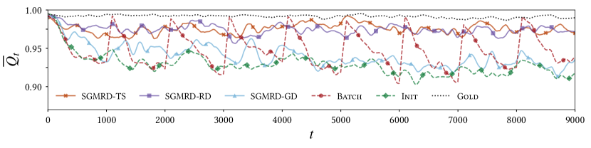
Figure 8. Average Quality at time $t$ (Pyro, ${L}=1$, $v=2$).

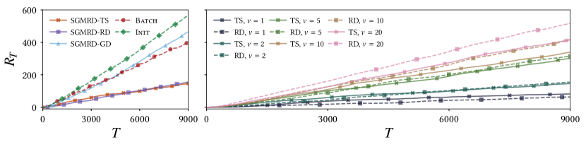
Figure 9. Regret up to $T$ (Pyro, ${L}=1$, left: $v=2$).

In Figure 10, the update frequencies give an intuition of how the three strategies differ. As expected, RD updates each subspace uniformly. GD tends to focus only on a few subspaces; most subspaces are never replaced, although they may become suboptimal as well. TS in turn tends to focus more on some subspaces, the ones requiring more frequent updates.

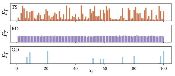
Figure 10. Frequency of update (Pyro, $v=2$, $L=1$).

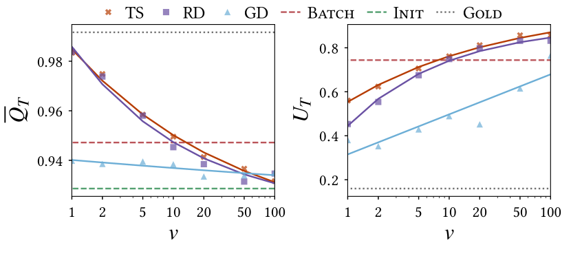
Figure 11. Quality and Success Rate w.r.t. $v$ (Pyro, ${L}=1$).

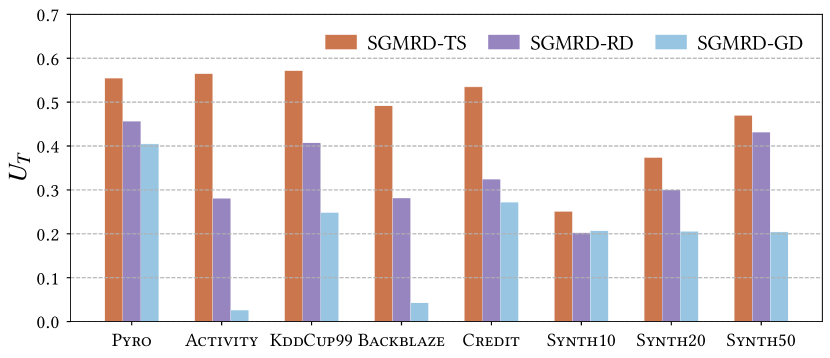
Figure 12. Success Rate (${L}=1$, $v=1$).

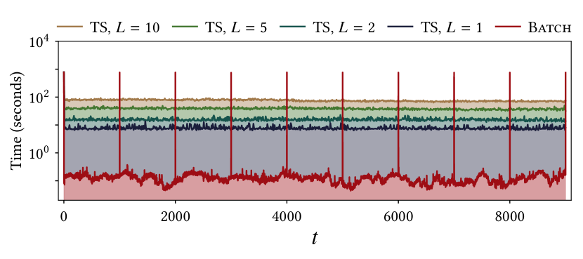
Figure 13. Stream Processing Time (Pyro, $v=1$).

Figure 11 shows that the average quality $\overline{Q}_{{T}}$ tends to decrease as we increase the update step $v$. However, the rate of successful updates $U_{{T}}$ (Equation 7) increases. As $v$ increases, it is more likely for any subspace to become suboptimal. For Batch, $U_{{T}}$ is high, but the quality $\overline{Q}_{{T}}$ is low. We observe the opposite for Gold. SGMRD is a trade-off between these two extremes, and the strategy based on TS appears superior to others, both w.r.t. $\overline{Q}_{{T}}$ and $U_{{T}}$. Figure 12 shows that our observations are not only valid for the Pyro data set, but also for other benchmarks. SGMRD-TS consistently achieves a higher rate of successful updates than other approaches.

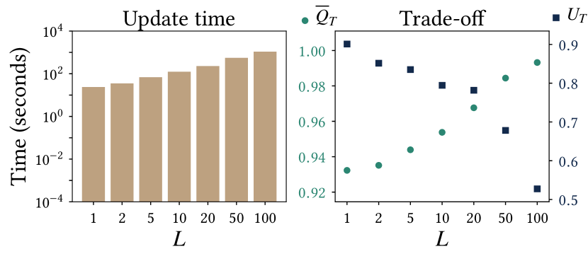
Figure 14. Quality/Efficiency (Pyro, SGMRD-TS, $v=100$).

Figure 13 highlights an important drawback of previous methods: The computation for batch-wise techniques is concentrated in a few discrete time steps. For stream mining, it is better to distribute computation uniformly over time. Computation-intensive episodes can lead to long response times of the system, and this contradicts the efficiency sought (C1) and anytime behaviour (C4). Besides this, the system becomes unable to adapt to the environment (C3).

Next, we set $v=100$ and let $L$ vary to observe the trade-off between quality of the subspaces and the efficiency of the search in SGMRD-TS (see Figure 14). As ${L}$ increases, the cost of updating subspaces increases linearly. Similarly, the quality $Q_{{T}}$ increases while the rate of successful updates $U_{{T}}$ decreases. As we can see in Table 2, SGMRD-TS has the highest quality after Gold, the best success rate $U_{{T}}$ after Batch and the smallest average regret among the baselines.

Table 2. Comparison design alternatives (Pyro, $v=1$).

Baseline	$L_{{T}}$	$\overline{Q}_{{T}}$	$U_{{T}}$	$R_{{T}}/T$
SGMRD-TS	1	95.43	0.61	3.74
SGMRD-RD	1	95.20	0.54	3.97
SGMRD-GD	1	93.72	0.43	5.45
Batch	NA	95.16	0.81	4.01
Init	NA	92.50	NA	6.67
Gold	100	99.16	0.16	NA

In conclusion, the experiments show that SGMRD is a useful tool to monitor high-quality subspaces over time, and it is highly versatile. Based on the available hardware, users can set the number of updates per round, as with SGMRD-TS, to obtain the highest quality for this budget. In the next section, we show that SGMRD-TS helps to detect outliers and compare the results with state-of-the-art outlier detectors for data streams.

7.2. Outlier Detection

Table 3. Outlier Detection Performance.

	Approach	AUC	AP	P1%	P2%	P5%	R1%	R2%	R5%
Activity	SGMRD	97.32	85.39	94.59	94.83	94.24	9.44	18.97	47.10
	LOF	93.93	61.80	74.32	64.72	64.03	7.42	12.94	32.00
	StreamHiCS	88.52	47.38	70.72	54.61	51.89	7.06	10.92	25.93
	RS-Stream	95.95	68.23	71.62	72.58	75.00	7.15	14.52	37.48
	xStream	77.71	20.41	3.60	10.14	16.31	0.36	2.02	8.13
KddCup99	SGMRD	69.98	10.29	0.00	0.20	0.56	0.00	0.06	0.39
	LOF	65.07	9.57	0.00	0.00	0.08	0.00	0.00	0.06
	StreamHiCS	57.11	7.89	0.00	0.00	0.08	0.00	0.00	0.06
	RS-Stream	43.21	5.73	0.00	0.00	0.08	0.00	0.00	0.06
	xStream	52.70	8.23	0.00	0.20	0.08	0.00	0.06	0.06
Backblaze	SGMRD	90.91	13.31	7.14	18.65	15.40	7.14	37.30	76.98
	LOF	56.92	1.65	2.38	3.57	2.38	2.38	7.14	11.90
	StreamHiCS	79.22	40.07	50.79	26.59	10.95	50.79	53.17	54.76
	RS-Stream	80.55	7.17	7.14	13.49	9.37	7.14	26.98	46.83
	xStream	76.86	3.69	1.59	3.17	6.19	1.59	6.35	30.95
Credit	SGMRD	95.06	15.87	10.69	7.47	3.22	55.51	77.57	83.65
	LOF	91.50	4.67	6.22	5.20	2.69	32.32	53.99	69.96
	StreamHiCS	89.21	3.48	3.59	2.93	2.28	18.63	30.42	59.32
	RS-Stream	85.13	1.63	2.27	2.49	1.86	11.79	25.86	48.29
	xStream	94.62	9.10	10.83	6.48	3.18	56.27	67.30	82.51
Synth10	SGMRD	92.70	59.93	50.00	26.00	12.00	58.14	60.47	69.77
	LOF	88.77	31.44	33.00	18.50	10.40	38.37	43.02	60.47
	StreamHiCS	88.81	31.16	33.00	19.00	10.40	38.37	44.19	60.47
	RS-Stream	71.23	1.87	0.00	0.00	2.80	0.00	0.00	16.28
	xStream	68.51	2.58	5.00	3.00	4.00	5.81	6.98	23.26
Synth20	SGMRD	85.05	41.19	36.00	19.50	9.20	40.91	44.32	52.27
	LOF	72.55	5.57	8.00	6.00	4.40	9.09	13.64	25.00
	StreamHiCS	71.71	5.37	8.00	6.00	4.00	9.09	13.64	22.73
	RS-Stream	48.39	0.80	0.00	0.00	0.00	0.00	0.00	0.00
	xStream	63.64	1.58	1.00	1.50	2.20	1.14	3.41	12.50
Synth50	SGMRD	75.87	31.27	27.00	16.00	7.60	33.33	39.51	46.91
	LOF	61.38	1.08	0.00	0.50	0.60	0.00	1.23	3.70
	StreamHiCS	63.90	12.00	11.00	6.00	3.40	13.58	14.81	20.99
	RS-Stream	46.52	0.73	0.00	0.00	0.00	0.00	0.00	0.00
	xStream	48.43	0.90	1.00	0.50	1.40	1.23	1.23	8.64

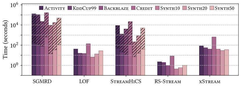
Figure 15. Outlier Detection Time (hatched: search time).

We leverage the subspaces obtained from SGMRD-TS to detect outliers, as in Section 5.2. We set ${w}=1000$, $v=1$ and ${L}=1$. Table 3 shows the results. Compared to our competitors, SGMRD clearly leads to the best results w.r.t. each benchmark. Interestingly, StreamHiCS appears to have higher recall and precision in the top 1-2%. We can see that LOF turns out to be our most competitive baseline and often outperforms our competitors.

In Figure 15, we can see that our competitors, in particular RS-Stream and xStream, are much faster than SGMRD, but they often are not much better than random guessing. Most of the computation required by SGMRD and StreamHiCS is due to the search. Nonetheless, one may reduce the required computation with SGMRD, e.g., increase $v$, without decreasing detection quality by much.

8. Conclusions

Finding interesting subspaces is fundamental to any step of the knowledge discovery process. We have proposed a new method, SGMRD, to bring subspace search to streams. It does so by combining an efficient greedy heuristic with novel multivariate quality estimators and an efficient bandit-based strategy, to update the results of subspace search over time.

Our experiments not only show that SGMRD leads to efficient monitoring of subspaces, but also to state-of-the-art results w.r.t. downstream data mining tasks, such as outlier detection, and one may expect similar benefits for other mining tasks on data streams.

An administrator can control monitoring via two parameters: the number of plays per round $L$ and the step size $v$. While the impact of a parameter value can be studied empirically, finding the most adequate parameters for a specific problem is not trivial. In future work, it would be interesting to extend our update policy in order to automatically tune those parameters, and to deal with their potential non-stationarity in the streaming setting. A possible direction is to leverage the recent bandit models from (Fouché et al., 2019).

- (1)
- Aggarwal (2009) Charu C. Aggarwal. 2009. On High Dimensional Projected Clustering of Uncertain Data Streams. In ICDE. IEEE Computer Society, 1152–1154. https://doi.org/10.1109/ICDE.2009.188
- Aggarwal (2013) Charu C. Aggarwal. 2013. Outlier Analysis. Springer. https://doi.org/10.1007/978-1-4614-6396-2
- Aggarwal and Sathe (2015) Charu C. Aggarwal and Saket Sathe. 2015. Theoretical Foundations and Algorithms for Outlier Ensembles. SIGKDD Explorations 17, 1 (2015), 24–47. https://doi.org/10.1145/2830544.2830549
- Agrawal et al. (2005) Rakesh Agrawal, Johannes Gehrke, Dimitrios Gunopulos, and Prabhakar Raghavan. 2005. Automatic Subspace Clustering of High Dimensional Data. Data Min. Knowl. Discov. 11, 1 (2005), 5–33. https://doi.org/10.1007/s10618-005-1396-1
- Assent et al. (2007) Ira Assent, Ralph Krieger, Emmanuel Müller, and Thomas Seidl. 2007. VISA: Visual Subspace Clustering Analysis. SIGKDD Explorations 9, 2 (2007), 5–12. https://doi.org/10.1145/1345448.1345451
- Bacher et al. (2016) M. Bacher, I. Ben-Gal, and E. Shmueli. 2016. Subspace selection for anomaly detection: An information theory approach. In 2016 IEEE International Conference on the Science of Electrical Engineering (ICSEE). 1–5. https://doi.org/10.1109/ICSEE.2016.7806077
- Barddal et al. (2015) Jean Paul Barddal, Heitor Murilo Gomes, and Fabrício Enembreck. 2015. A Survey on Feature Drift Adaptation. In ICTAI. IEEE Computer Society, 1053–1060. https://doi.org/10.1109/ICTAI.2015.150
- Baumgartner et al. (2004) Christian Baumgartner, Claudia Plant, Karin Kailing, Hans-Peter Kriegel, and Peer Kröger. 2004. Subspace Selection for Clustering High-Dimensional Data. In ICDM. IEEE Computer Society, 11–18. https://doi.org/10.1109/ICDM.2004.10112
- Becker (2016) Vincent Becker. 2016. Concept Change Detection in Correlated Subspaces in Data Streams. Master’s thesis. Karlsruhe Institute of Technology.
- Breunig et al. (2000) Markus M. Breunig, Hans-Peter Kriegel, Raymond T. Ng, and Jörg Sander. 2000. LOF: Identifying Density-Based Local Outliers. In SIGMOD Conference. ACM, 93–104. https://doi.org/10.1145/342009.335388
- Bubeck and Cesa-Bianchi (2012) Sébastien Bubeck and Nicolò Cesa-Bianchi. 2012. Regret Analysis of Stochastic and Nonstochastic Multi-armed Bandit Problems. Foundations and Trends in Machine Learning 5, 1 (2012), 1–122. https://doi.org/10.1561/2200000024
- C. et al. (2017) Carlos A. Rincon C., Jehan-François Pâris, Ricardo Vilalta, Albert M. K. Cheng, and Darrell D. E. Long. 2017. Disk failure prediction in heterogeneous environments. In SPECTS. IEEE, 1–7.
- Campos et al. (2016) Guilherme O. Campos, Arthur Zimek, Jörg Sander, Ricardo J. G. B. Campello, Barbora Micenková, Erich Schubert, Ira Assent, and Michael E. Houle. 2016. On the Evaluation of Unsupervised Outlier Detection: Measures, Datasets, and an Empirical Study. Data Min. Knowl. Discov. 30, 4 (2016), 891–927. https://doi.org/10.1007/s10618-015-0444-8
- Chapelle and Li (2011) Olivier Chapelle and Lihong Li. 2011. An Empirical Evaluation of Thompson Sampling. In NIPS. 2249–2257. https://dl.acm.org/doi/10.5555/2986459.2986710
- Domingos and Hulten (2003) Pedro Domingos and Geoff Hulten. 2003. A General Framework for Mining Massive Data Streams. Journal of Computational and Graphical Statistics 12, 4 (2003), 945–949. https://doi.org/10.1198/1061860032544
- Dua and Graff (2017) Dheeru Dua and Casey Graff. 2017. UCI Machine Learning Repository. http://archive.ics.uci.edu/ml
- Fouché and Böhm (2019) Edouard Fouché and Klemens Böhm. 2019. Monte Carlo Dependency Estimation. In SSDBM. ACM, 13–24. https://doi.org/10.1145/3335783.3335795
- Fouché et al. (2019) Edouard Fouché, Junpei Komiyama, and Klemens Böhm. 2019. Scaling Multi-Armed Bandit Algorithms. In KDD. ACM, 1449–1459. https://doi.org/10.1145/3292500.3330862
- Fouché et al. (2020) Edouard Fouché, Alan Mazankiewicz, Florian Kalinke, and Klemens Böhm. 2020. A Framework for Dependency Estimation in Heterogeneous Data Streams. DAPD journal (2020). https://doi.org/10.1007/s10619-020-07295-x
- Gama (2012) João Gama. 2012. A survey on learning from data streams: current and future trends. Progress in AI 1, 1 (2012), 45–55. https://doi.org/10.1007/s13748-011-0002-6
- Gupta et al. (2014) Manish Gupta, Jing Gao, Charu C. Aggarwal, and Jiawei Han. 2014. Outlier Detection for Temporal Data: A Survey. IEEE Trans. Knowl. Data Eng. 26, 9 (2014), 2250–2267. https://doi.org/10.1109/TKDE.2013.184
- Guyon and Elisseeff (2003) Isabelle Guyon and André Elisseeff. 2003. An Introduction to Variable and Feature Selection. J. Mach. Learn. Res. 3 (2003), 1157–1182. http://jmlr.org/papers/v3/guyon03a.html
- Hoeffding (1963) Wassily Hoeffding. 1963. Probability Inequalities for Sums of Bounded Random Variables. J. Amer. Statist. Assoc. 58, 301 (1963), 13–30. https://doi.org/10.1080/01621459.1963.10500830
- Joe (1989) Harry Joe. 1989. Relative Entropy Measures of Multivariate Dependence. J. Amer. Statist. Assoc. 84, 405 (1989), 157–164. https://doi.org/10.2307/2289859
- Kailing et al. (2003) Karin Kailing, Hans-Peter Kriegel, Peer Kröger, and Stefanie Wanka. 2003. Ranking Interesting Subspaces for Clustering High Dimensional Data. In PKDD (Lecture Notes in Computer Science, Vol. 2838). Springer, 241–252. https://doi.org/10.1007/978-3-540-39804-2_23
- Kaufmann et al. (2012) Emilie Kaufmann, Nathaniel Korda, and Rémi Munos. 2012. Thompson Sampling: An Asymptotically Optimal Finite-Time Analysis. In ALT (Lecture Notes in Computer Science, Vol. 7568). Springer, 199–213. https://doi.org/10.1007/978-3-642-34106-9_18
- Keller et al. (2012) Fabian Keller, Emmanuel Müller, and Klemens Böhm. 2012. HiCS: High Contrast Subspaces for Density-Based Outlier Ranking. In ICDE. IEEE Computer Society, 1037–1048. https://doi.org/10.1109/ICDE.2012.88
- Komiyama et al. (2015) Junpei Komiyama, Junya Honda, and Hiroshi Nakagawa. 2015. Optimal Regret Analysis of Thompson Sampling in Stochastic Multi-armed Bandit Problem with Multiple Plays. In ICML (JMLR Workshop and Conference Proceedings, Vol. 37). JMLR.org, 1152–1161. http://proceedings.mlr.press/v37/komiyama15.html
- Kontaki et al. (2006) Maria Kontaki, Apostolos N. Papadopoulos, and Yannis Manolopoulos. 2006. Efficient Incremental Subspace Clustering in Data Streams. In IDEAS. IEEE Computer Society, 53–60. https://doi.org/10.1109/IDEAS.2006.19
- Kriegel et al. (2009) Hans-Peter Kriegel, Peer Kröger, and Arthur Zimek. 2009. Clustering High-Dimensional Data: A Survey on Subspace Clustering, Pattern-Based Clustering, and Correlation Clustering. TKDD 3, 1 (2009), 1:1–1:58. https://doi.org/10.1145/1497577.1497578
- Lazarevic and Kumar (2005) Aleksandar Lazarevic and Vipin Kumar. 2005. Feature Bagging for Outlier Detection. In KDD. ACM, 157–166. https://doi.org/10.1145/1081870.1081891
- Manzoor et al. (2018) Emaad Manzoor, Hemank Lamba, and Leman Akoglu. 2018. xStream: Outlier Detection in Feature-Evolving Data Streams. In KDD. ACM, 1963–1972. https://doi.org/10.1145/3219819.3220107
- Nguyen (2015) Hoang Vu Nguyen. 2015. Non-parametric Methods for Correlation Analysis in Multivariate Data with Applications in Data Mining. Ph.D. Dissertation. Karlsruhe Institute of Technology. https://doi.org/10.5445/IR/1000049548
- Nguyen et al. (2016b) Hoang Vu Nguyen, Panagiotis Mandros, and Jilles Vreeken. 2016b. Universal Dependency Analysis. In SDM. SIAM, 792–800. https://doi.org/10.1137/1.9781611974348.89
- Nguyen et al. (2016a) Xuan Vinh Nguyen, Jeffrey Chan, Simone Romano, James Bailey, Christopher Leckie, Kotagiri Ramamohanarao, and Jian Pei. 2016a. Discovering outlying aspects in large datasets. Data Min. Knowl. Discov. 30, 6 (2016), 1520–1555. https://doi.org/10.1007/s10618-016-0453-2
- Park and Lee (2007) Nam Hun Park and Won Suk Lee. 2007. Grid-based Subspace Clustering over Data Streams. In CIKM. ACM, 801–810. https://doi.org/10.1145/1321440.1321551
- Parsons et al. (2004) Lance Parsons, Ehtesham Haque, and Huan Liu. 2004. Subspace Clustering for High Dimensional Data: A Review. SIGKDD Explorations 6, 1 (2004), 90–105. https://doi.org/10.1145/1007730.1007731
- Pokrajac et al. (2007) Dragoljub Pokrajac, Aleksandar Lazarevic, and Longin Jan Latecki. 2007. Incremental Local Outlier Detection for Data Streams. In CIDM. IEEE, 504–515. https://doi.org/10.1109/CIDM.2007.368917
- Pozzolo et al. (2018) Andrea Dal Pozzolo, Giacomo Boracchi, Olivier Caelen, Cesare Alippi, and Gianluca Bontempi. 2018. Credit Card Fraud Detection: A Realistic Modeling and a Novel Learning Strategy. IEEE Trans. Neural Networks Learn. Syst. 29, 8 (2018), 3784–3797.
- Procopiuc et al. (2002) Cecilia Magdalena Procopiuc, Michael Jones, Pankaj K. Agarwal, and T. M. Murali. 2002. A Monte Carlo Algorithm for Fast Projective Clustering. In SIGMOD Conference. ACM, 418–427. https://doi.org/10.1145/564691.564739
- Reiss and Stricker (2012) Attila Reiss and Didier Stricker. 2012. Introducing a New Benchmarked Dataset for Activity Monitoring. In ISWC. IEEE Computer Society, 108–109. https://doi.org/10.1109/ISWC.2012.13
- Sathe and Aggarwal (2016) Saket Sathe and Charu C. Aggarwal. 2016. Subspace Outlier Detection in Linear Time with Randomized Hashing. In ICDM. IEEE Computer Society, 459–468. https://doi.org/10.1109/ICDM.2016.0057
- Sathe and Aggarwal (2018) Saket Sathe and Charu C. Aggarwal. 2018. Subspace histograms for outlier detection in linear time. Knowl. Inf. Syst. 56, 3 (2018), 691–715. https://doi.org/10.1007/s10115-017-1148-8
- Schubert et al. (2015) Erich Schubert, Alexander Koos, Tobias Emrich, Andreas Züfle, Klaus Arthur Schmid, and Arthur Zimek. 2015. A Framework for Clustering Uncertain Data. PVLDB 8, 12 (2015), 1976–1979. https://doi.org/10.14778/2824032.2824115
- Siegel and Castellan (1988) S. Siegel and N.J. Castellan. 1988. Nonparametric Statistics for the Behavioral Sciences (2 ed.). McGraw-Hill.
- Tatu et al. (2012) Andrada Tatu, Fabian Maass, Ines Färber, Enrico Bertini, Tobias Schreck, Thomas Seidl, and Daniel Keim. 2012. Subspace Search and Visualization to Make Sense of Alternative Clusterings in High-Dimensional Data. In IEEE VAST. IEEE Computer Society, 63–72. https://doi.org/10.1109/VAST.2012.6400488
- Thompson (1933) William R. Thompson. 1933. On the Likelihood that One Unknown Probability Exceeds Another in View of the Evidence of Two Samples. Biometrika 25, 3/4 (1933), 285–294. https://doi.org/10.2307/2332286
- Trittenbach and Böhm (2019) Holger Trittenbach and Klemens Böhm. 2019. Dimension-based subspace search for outlier detection. Int. J. Data Sci. Anal. 7, 2 (2019), 87–101. https://doi.org/10.1007/s41060-018-0137-7
- Vanea et al. (2012) Andrei Vanea, Emmanuel Müller, Fabian Keller, and Klemens Böhm. 2012. Instant Selection of High Contrast Projections in Multi-Dimensional Data Streams. In Proceedings of the Workshop on Instant Interactive Data Mining (IID 2012) in conjunction with ECML PKDD.
- Wang et al. (2017) Yisen Wang, Simone Romano, Vinh Nguyen, James Bailey, Xingjun Ma, and Shu-Tao Xia. 2017. Unbiased Multivariate Correlation Analysis. In AAAI. AAAI Press, 2754–2760. http://aaai.org/ocs/index.php/AAAI/AAAI17/paper/view/14214
- Zhang et al. (2008) Ji Zhang, Qigang Gao, and Hai H. Wang. 2008. SPOT: A System for Detecting Projected Outliers From High-dimensional Data Streams. In ICDE. IEEE Computer Society, 1628–1631. https://doi.org/10.1109/ICDE.2008.4497638
- Zhang et al. (2007) Qi Zhang, Jinze Liu, and Wei Wang. 2007. Incremental Subspace Clustering over Multiple Data Streams. In ICDM. IEEE Computer Society, 727–732. https://doi.org/10.1109/ICDM.2007.100
- Zimek et al. (2012) Arthur Zimek, Erich Schubert, and Hans-Peter Kriegel. 2012. A Survey on Unsupervised Outlier Detection in High-Dimensional Numerical Data. Statistical Analysis and Data Mining 5, 5 (2012), 363–387. https://doi.org/10.1002/sam.11161