Notes on AdS-Schwarzschild eikonal phase

Abstract

We consider the eikonal phase associated with the gravitational scattering of a highly energetic light particle off a very heavy object in AdS spacetime. A simple expression for this phase follows from the WKB approximation to the scattering amplitude and has been computed to all orders in the ratio of the impact parameter to the Schwarzschild radius of the heavy particle. The eikonal phase is related to the deflection angle by the usual stationary phase relation. We consider the flat space limit and observe that for sufficiently small impact parameters (or angular momenta) the eikonal phase develops a large imaginary part; the inelastic cross-section is exactly the classical absorption cross-section of the black hole. We also consider a double scaling limit where the momentum becomes null simultaneously with the asymptotically AdS black hole becoming very large. In the dual CFT this limit retains contributions from all leading twist multi stress tensor operators, which are universal with respect to the addition of higher derivative terms to the gravitational lagrangian. We compute the eikonal phase and the associated Lyapunov exponent in the double scaling limit.

1 Introduction and Summary

1.1 Introduction

Gravitational high-energy scattering probes an interesting regime of quantum gravity. At large impact parameters (very small momentum transfer) the scattering amplitude is given by a single graviton exchange. As the impact parameter is lowered, the amplitude is related by a Fourier transform in the impact parameter space to the exponential of the eikonal phase (see e.g. Giddings:2011xs for a review). As the impact parameter $b$ becomes comparable with the Schwarzschild radius $R_{s}$ associated with the total energy, a black hole may form – this is reflected in the imaginary part of the eikonal phase. These issues have been a subject of active investigation starting from tHooft:1987vrq ; Amati:1987wq ; Muzinich:1987in ; Sundborg:1988tb ; Amati:1987uf ; Amati:1990xe ; Verlinde:1991iu . For example, ref. Giddings:2007qq advocated a black hole ansatz to describe the breakdown of unitarity. Generally one needs the full eikonal phase, to all orders in the ratio $R_{s}/b$, to study the black hole regime.

A simplification happens when one of the particles is very heavy, so that its mass is the largest scale in the problem, and the other particle is highly relativistic. In this case the eikonal phase determines the deflection of null geodesics in the Schwarzschild background (see e.g. Kabat:1992tb ; DAppollonio:2010krb ; Neill:2013wsa ; Akhoury:2013yua ; Bjerrum-Bohr:2014zsa ; Bjerrum-Bohr:2016hpa ; Luna:2016idw ; Cachazo:2017jef ; Bjerrum-Bohr:2018xdl ; Cheung:2018wkq ; Kosower:2018adc ; Bern:2019nnu ; KoemansCollado:2019ggb ; Bern:2019crd ; Bjerrum-Bohr:2019kec ; Damour:2019lcq ; Bern:2020gjj ; Blumlein:2020znm ; Cheung:2020gyp ; Cristofoli:2020uzm ; Bini:2020wpo ; Bern:2020buy ; Parra-Martinez:2020dzs ; Kalin:2020mvi ; DiVecchia:2020ymx ; Damour:2020tta ; Cheung:2020gbf for some work related to the computation of the heavy-light scattering angle.) The deflection angle can in principle be computed to all orders in $R_{s}/b$.

A similar problem can be posed in AdS spacetime , where the eikonal phase (a.k.a. the phase shift) is an interesting object from the point of view of the holographically dual CFT. For example, in Giusto:2020mup the phase shift was used to distinguish black hole microstates from conical defects. In Kulaxizi:2018dxo it was argued that conformal two-point functions in a generic heavy state could be used to obtain the AdS-Schwarzschild eikonal phase. Moreover, the phase is only sensitive to the stress-tensor sector of the correlator, which only contains contributions from the stress tensor and its composites.

There has been some progress in computing the stress-tensor sector of such correlators Fitzpatrick:2019zqz ; Karlsson:2019qfi ; Li:2019tpf ; Kulaxizi:2019tkd ; Fitzpatrick:2019efk ; Karlsson:2019dbd ; Li:2019zba ; Karlsson:2019txu ; Karlsson:2020ghx ; Li:2020dqm ; Parnachev:2020fna ; Fitzpatrick:2020yjb . In particular, in Fitzpatrick:2019zqz the leading twist stress tensor OPE coefficients in holographic CFTs were shown to be largely universal – independent of the higher derivative terms in the bulk gravitational action. In Kulaxizi:2019tkd the contributions of all leading twist double stress tensors in such CFTs were shown to produce a very simple function. In Karlsson:2019dbd it was explained how the leading twist stress tensor sector can be computed by bootstrap and in Karlsson:2020ghx it was shown how to go beyond the leading twist – the phase shift played an important role in this story. So, the AdS-Schwarzschild eikonal phase is an important object. In this paper we discuss its properties and investigate various limits.

1.2 Summary and outline

As we review in Section 2, to compute the phase shift one needs to Fourier transform a heavy-heavy-light-light (HHLL) correlator on the boundary. The Fourier transformed correlator is a function of the energy, $p^{t}$, and the angular momentum $p^{\varphi}$. In the limit where $p^{t}$ and $p^{\varphi}$ are large, the eikonal phase can be computed exactly as a function of the ratio $\alpha=p^{\varphi}/p^{t}$, related to the impact parameter, and is given by Kulaxizi:2018dxo

$$\delta=p^{t}\Delta t-p^{\varphi}\Delta\varphi\,,$$ (1)

where $\Delta t$ and $\Delta\varphi$ are the time and angular displacements of the null geodesic with the energy $p^{t}$ and angular momentum $p^{\varphi}$.

As we describe in Section 2, this is simply a consequence of the WKB approximation to the differential equation which determines the holographic correlator. Another way to illustrate how eq. (1) emerges involves considering a probe particle with the mass which is large in AdS units. The two-point function is then determined by the length of spacelike geodesics and is peaked around points connected by null geodesics. Such points form a codimension one subspace on the boundary. There is a null geodesic which gives the dominant contribution. The parameters of this geodesic can be determined from the stationary phase condition – it is precisely the null geodesic whose energy and angular momentum are equal to the $p^{t}$ and $p^{\varphi}$ parameters of the Fourier transform. Hence, we end up with the expression (1) for the phase shift.

The AdS eikonal phase is directly related to the usual eikonal phase in the flat space scattering computed in the probe limit. To get the latter, one simply needs to take the flat space limit of the AdS result, which we do in Section 3. One can confirm that the resulting formula is the conventional flat space eikonal phase by considering the relation between the AdS phase shift and the deflection angle – this relation is exactly the same as the one which follows from the stationary phase approximation to the eikonal scattering amplitude in flat spacetimes.

The flat space limit yields a very simple formula for the eikonal phase, as we observe in Section 3. It can be summed to give an analytic function; we perform this summation in four spacetime dimensions. The resulting phase is real for impact parameters larger than the radius of the circular null orbit, but develops a large imaginary part for smaller impact parameters. As a result, the total inelastic cross-section is equal to the geometric absorption cross-section of the Schwarschild black hole.

In Section 4 we consider the opposite limit of large impact parameters. More precisely, we take a double scaling limit where the impact parameter becomes large (the momentum approaches the lightcone) and at the same time the Schwarzschild radius also becomes large in AdS units. This limit is particularly interesting from the dual CFT point of view – it retains contribution from all leading twist multi-stress tensors. We study the propagation of null geodesics in the the effective metric derived in Parnachev:2020fna and use eq. (1) to compute the phase shift. It agrees (as it should) with the corresponding limit of the full phase shift. We also compute the Lyapunov exponent for the null geodesics approaching the null orbit in the effective metric.

We discuss our results in Section 5. Appendices contain some technical details used in the main text.

2 Eikonal phase in AdS-Schwarzschild

Ref. Kulaxizi:2018dxo argued that two-point functions in certain heavy states in holographic CFTs with a large central charge $C_{T}$ can be used to define the eikonal phase (a.k.a. the phase shift). One should simply Fourier transform the CFT correlator on the $d$-dimensional Lorentzian cylinder (the boundary of the $d+1$ dimensional asymptotically AdS spacetime)

$$e^{i\delta}\simeq\int dtd\varphi\ e^{-ip^{t}t}\ (\sin\varphi)^{d-2}C_{p^{\varphi}}^{d-2\over 2}(\cos\varphi)\langle{\cal O}_{H}{\cal O}_{L}(t,\varphi){\cal O}_{L}(0){\cal O}_{H}\rangle\,,$$ (2)

where the heavy operators ${\cal O}_{H}$ (with the conformal dimension $\Delta_{H}\sim C_{T}$) are inserted at $t=\pm\infty$ and $t,\varphi$ are the displacements of the two light operators [with $\Delta_{L}\simeq{\cal O}(1)$] on the cylinder ($\varphi$ is the relative angle on the $d-1$-dimensional spatial sphere of radius $R$ ). In (2) $C_{p^{\varphi}}^{d-2\over 2}(\cos\varphi)$ are the Gegenbauer polynomials with the angular momentum $p^{\varphi}$ , which generalize the spherical harmonics of the $d=4$ case. The momenta are taken to be large, $p^{t}\gg R^{-1},p^{\varphi}\gg 1$ and the integral in (2) can be computed in the stationary phase approximation. Substituting the large $p^{\varphi}$ behavior of the Gegenbauer polynomials, (2) can be written as

$$e^{i\delta}\simeq\int dtd\varphi\ e^{-ip^{t}t+ip^{\varphi}\varphi}\ \langle{\cal O}_{H}{\cal O}_{L}(t,\varphi){\cal O}_{L}(0){\cal O}_{H}\rangle\,.$$ (3)

In the following we will mostly set $R=1$, but it can be easily recovered on dimensional grounds. Note that the phase shift, as defined by (2) is related to the eikonal phase $\delta_{\ell}$ conventionally appearing in the scattering amplitudes (see e.g. Soldate:1986mk ; Giddings:2007qq ; Damour:2019lcq ; Bern:2020gjj ) by a factor of two,

$$\delta=2\delta_{\ell}\,.$$ (4)

The Fourier transformed correlator in the large $p^{t},p^{\varphi}$ limit receives a dominant contribution from a certain null geodesic, as we review below. It was argued in Kulaxizi:2018dxo that the phase shift is given by (1) where $p^{t}$ and $p^{\varphi}$ are now the conserved quantities which determine the trajectory of the corresponding null geodesic, while $\Delta t$ and $\Delta\varphi$ describe the deviation of the point where the null geodesic emerges at the boundary of the AdS-Schwarzschild from the pure AdS result. The explicit expression for the phase shift in the $D=d+1$-dimensional AdS-Schwarzschild spacetime is Kulaxizi:2018dxo

$$\begin{split}\delta(\sqrt{-p^{2}},\,L)&{=}\sum_{k=0}^{\infty}\delta_{k}(\sqrt{-p^{2}},\,L){=}\\ &{=}\sum_{k=1}^{\infty}{\mu^{k}\over k!}\,{2\Gamma\left[{dk+1\over 2}\right]\over\Gamma\left[{k(d-2)+1\over 2}\right]}\,{\pi^{k(d-2)+2\over 2}\over\Gamma[{k(d-2)+2\over 2}]}\,\,\,\sqrt{-p^{2}}\,\,\Pi_{k(d-2)+1,k(d-2)+1}(L)\,.\end{split}$$ (5)

where

$$\Pi_{\Delta-1;d-1}(x)={\pi^{1-{d\over 2}}\Gamma(\Delta-1)\over 2\Gamma(\Delta-{d-2\over 2})}\ e^{-(\Delta-1)x}\ _{2}F_{1}({d\over 2}-1,\Delta-1,\Delta-{d\over 2}+1,e^{-2x})\,.$$ (6)

and

$$e^{2L}={p^{+}\over p^{-}}={p^{t}+p^{\varphi}\over p^{t}-p^{\varphi}}\,.$$ (7)

In (5) and in the rest of the paper $\mu$ is proportional to the mass of the AdS-Schwarzschild black hole $M$ and to the ratio $\Delta_{H}/C_{T}$,

$$\mu=\left[{d-1\over 16\pi}\Omega_{d-1}\right]^{-1}G_{N}M={4\Gamma(d+2)\over(d-1)^{2}\Gamma({d\over 2})}\ {\Delta_{H}\over C_{T}}$$ (8)

where $G_{N}$ is the $d+1$-dimensional Newton’s constant and $\Omega_{d-1}$ is the volume of the $d-1$-dimensional sphere.

2.1 The phase shift formula from the WKB approximation

In this subsection we use the WKB approximation for the two-point function in the (thermal) CFT state dual to the AdS-Schwarzschild background to show that the phase shift is given by (1). (See e.g. Festuccia:2008zx and also Balasubramanian:2019stt ; Craps:2020ahu for examples of a WKB approximation in the computation of a two-point funciton).

In a $d+1$-dimensional AdS-Schwarzschild spacetime,

$$ds^{2}=-f(r)dt^{2}+{dr^{2}\over f(r)}+r^{2}d\Omega_{d-1}\,,$$ (9)

with $f=1-r^{2}+\mu/r^{d-2}$, the time delay and the anglular deflection of null geodesics are given by

$$\Delta t=2p^{t}\int_{r_{0}}^{\infty}{dr\over f(r)\ \sqrt{1-{f(r)\alpha^{2}\over r^{2}}}},\quad\Delta\varphi=2p^{\varphi}\alpha\int_{r_{0}}^{\infty}{dr\over r^{2}\ \sqrt{1-{f(r)\alpha^{2}\over r^{2}}}}\,,$$ (10)

where $p^{t}$ ($p^{\varphi}$) is the energy (angular momentum), $\alpha=p^{\varphi}/p^{t}$ and $r_{0}$ is the largest solution of $f(r)\alpha^{2}=r^{2}$. One can now use (1) to arrive at the following formula for the phase shift

$$\delta=2|p^{t}|\int_{r_{0}}^{\infty}{dr\over f(r)}\ \sqrt{1-{f(r)\alpha^{2}\over r^{2}}}\,.$$ (11)

Consider now a holographic two-point function in the thermal state (9). The action for a massive scalar is given by

$$S\simeq\int d^{5}x\sqrt{-\det g_{\alpha\beta}}\;\left[g^{\mu\nu}\partial_{\mu}\phi\partial_{\nu}\phi-m^{2}\phi^{2}\right]\,.$$ (12)

As usual, the mass is related to the conformal dimension of the dual scalar operator by the AdS/CFT correspondence Maldacena:1997re ; Witten:1998qj ; Gubser:1998bc via $m^{2}R^{2}={\Delta_{L}}({\Delta_{L}}-d)$. The equation of motion is

$$r^{1-d}\partial_{r}(r^{d-1}f\partial_{r}\phi)-f^{-1}\partial_{t}^{2}\phi+r^{-2}\partial_{\varphi}^{2}\phi+m^{2}\phi=0\,.$$ (13)

Performing the Fourier transform to $\tilde{\phi}(p^{t},p^{\varphi})$, substituting

$$\tilde{\phi}(p^{t},p^{\varphi})=e^{ip^{t}\psi}$$ (14)

and retaining the leading terms in the large energy limit, $p^{t},p^{\varphi}\gg 1,m$, yields

$$(\partial_{r}\psi)^{2}={1\over f^{2}(r)}\left(1-{\alpha^{2}f(r)\over r^{2}}\right)\,,$$ (15)

which can be integrated and gives precisely (11) for the phase shift.

2.2 Null geodesics and the phase shift

It is not hard to prove the following identity for the null geodesics, by performing direct differentiation of both the lower limit of integration and the integrands,

$$\alpha{\partial\over\partial\alpha}\int_{r_{0}}^{\infty}{\alpha dr\over r^{2}\sqrt{1-{f(r)\alpha^{2}\over r^{2}}}}-{\partial\over\partial\alpha}\int_{r_{0}}^{\infty}{dr\over f(r)\sqrt{1-{f(r)\alpha^{2}\over r^{2}}}}=0\,.$$ (16)

With this identity, one can further show that

$$\Delta t={\partial\delta\over\partial p^{t}},\qquad\Delta\varphi=-{\partial\delta\over\partial p^{\varphi}}\,.$$ (17)

Equations (17) generalize the result of Appendix E in Karlsson:2020ghx . Note that (17) are exactly the relations between the eikonal phase and the time delay and angular deflection, familiar from the Regge scattering in flat spacetime [they follow from the stationary phase approximation for the scattering amplitude; one should also bear in mind a factor of two in (4) ].

The identity (16) can be used to illustrate how eq. (1) emerges from the Fourier transform of the correlator in the large $\Delta_{L}$ limit. In this limit, the two-point function is related to the length of a geodesic which connects two points on the boundary. At large momenta, the dominant contribution comes from null geodesics, since they minimize the length (see e.g. Hubeny:2006yu for a related discussion). There is one specific null geodesic which extremizes the phase shift – its parameters can be determined by the stationary phase consition. We need to extremize

$${\delta\over p^{t}}=\int_{r_{0}}^{\infty}{dr\over f(r)\ \sqrt{1-{f(r)\alpha^{2}\over r^{2}}}}-{p^{\varphi}\over p^{t}}\alpha\int_{r_{0}}^{\infty}{dr\over r^{2}\ \sqrt{1-{f(r)\alpha^{2}\over r^{2}}}}$$ (18)

with respect to the parameter $\alpha$, which labels null geodesics. In (18) the ratio of the external momenta $p^{\varphi}/p^{t}$ is fixed ( $p^{\varphi}$ and $p^{t}$ are simply the variables of the Fourier transform).

According to (16) the extremum is achieved for the value of $\alpha$ which is precisely equal to the ratio $p^{\varphi}/p^{t}$, thereby confirming (1).

3 Flat space limit (small AdS impact parameter)

3.1 Taking the flat space limit

It is interesting to take the flat space limit of (5). This is achieved by taking the AdS radius $R$ to be large compared to the Schwarzschild radius $R_{s}$ of the black hole and the impact parameter $b$. Recall that Kulaxizi:2018dxo

$$b=R\ \sinh L,\qquad\mu\approx\left({R_{s}\over R}\right)^{D-3}\,.$$ (19)

Hence, the flat space limit corresponds to the limit of small $\mu$ and $L$ with

$${\mu\over L^{D-3}}\approx\left({R_{s}\over b}\right)^{D-3}\approx\left({R_{s}p^{t}\over p^{\varphi}}\right)^{D-3}$$ (20)

fixed. The result of this limit for the phase shift is

$$\delta_{M}=\sum_{k=1}^{\infty}{\sqrt{\pi}\Gamma\left({(D-1)k+1\over 2}\right)\over((D-3)k-1)k!\Gamma\left({(D-3)k\over 2}+1\right)}{(R_{s}p^{t})^{k(D-3)}\over(p^{\varphi})^{k(D-3)-1}}\,,$$ (21)

where the subscript ”M” stands for Minkowski spacetime. It is instructive to compute the deflection angle,

$$\varphi_{M}=-{d\delta_{M}\over dp^{\varphi}}\,.$$ (22)

Differentiating eq. (21) yields

$$\varphi_{M}=\sum_{k=1}^{\infty}{\sqrt{\pi}\Gamma\left({(D-1)k+1\over 2}\right)\over k!\Gamma\left({(D-3)k\over 2}+1\right)}\left({R_{s}\over b}\right)^{k(D-3)}$$ (23)

where we substituted $b=p^{\varphi}/p^{t}$.

3.2 Four-dimensional spacetime

Consider the four-dimensional spacetime, $D=4$. As an extra check, we can make use of eq. (11.32) in Bern:2019crd (see also appendix D of KoemansCollado:2019ggb ) where the scattering angle is quoted up to the next-to-next to leading order. To compare with our results, we need to take the probe limit, where the mass of one particle is the largest scale in the problem. This produces

$$\varphi_{M}=2\left({R_{s}\over b}\right)+{15\pi\over 16}\left({R_{s}\over b}\right)^{2}+{16\over 3}\left({R_{s}\over b}\right)^{3}+\ldots\,.$$ (24)

This is in complete agreement with (23).

It is interesting that the sum in (21) can be computed exactly. One way to do it is to substitute $D=4$ in (23) and then integrate the result. It will be convenient to define

$$x={3\sqrt{3}\over 2}\ {R_{s}p^{t}\over p^{\varphi}}\,,$$ (25)

which yields

$$\delta_{M}={3\sqrt{3}R_{s}p^{t}\over 2x}\left(i\pi-\pi\ _{3}F_{2}[-\frac{1}{2},\frac{1}{6},\frac{5}{6};\frac{1}{2},1;x^{2}]-{x\over 4}G^{2,3}_{4,4}[-\frac{1}{3},0,\frac{1}{3},1;0,0,-\frac{1}{2},-\frac{1}{2};-x^{2}]\right)+c\,,$$ (26)

where $G^{2,3}_{4,4}$ is the Meijer G-function (see Appendix A) and $c$ is a real constant. We will be interested in the imaginary part of the phase shift, which develops for $x>1$ (this corresponds to the impact parameter of a null geodesic which approaches the light orbit).

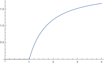
Figure 1: The plot of $Im\delta_{M}/(R_{s}p^{t}\pi)$

It has the form (see Appendix A)

$$Im\ \delta_{M}=R_{s}p^{t}f(x)\,,$$ (27)

where $f(x)$ is plotted in Fig. 1. The imaginary part is vanishing (the scattering is elastic) for $x<1$ which corresponds to the impact parameter larger than the radius of the circular light orbit, $R_{*}=3\sqrt{3}R_{s}/2$. On the other hand, for $x>1$, $Im\ \delta_{M}$ is very large (since $R_{s}p^{t}\gg 1$ in the eikonal limit we consider) - the scattering for these partial waves is completely non-elastic (they are totally absorbed). The inelastic scattering cross-section is

$$\sigma_{in,M}={\pi\over(p^{t})^{2}}\sum_{\ell=0}^{p^{t}R_{*}}(2\ell+1)(1-|e^{i\delta}|^{2})=\pi R_{*}^{2}\,.$$ (28)

This is the geometric absorption cross-section of the Schwarzschild metric.

4 Leading twist limit (large AdS impact parameter)

Each term in the phase shift result (5) has the following behavior in the large impact parameter regime, $L\gg 1$,

$$\delta^{(k)}(p^{2},L)\sim\sqrt{-p^{2}}e^{-(k(d-2)+1)L}\sim p^{-}e^{-k(d-2)L}\,,$$ (29)

which summarizes the contributions of all leading twist k-stress tensors. Hence, one can take a double scaling limit $\mu\rightarrow\infty$, $\mu e^{-(d-2)L}$ fixed, where only such operators survive.

This limit was recently considered in Parnachev:2020fna , where an effective three-dimensional metric with the boundary coordinates $x^{+}=t+\varphi$, $x^{-}=\mu^{2\over d-2}(t-\varphi)$ was introduced. It is clear that one should be able to recover (38) directly from that effective metric,

$$\delta={1\over 2}p^{+}(\Delta t-\Delta\varphi)+{1\over 2}p^{-}{\Delta x^{+}}={p^{-}\over 2}\left({p^{+}\over\mu^{2\over d-2}p^{-}}{\Delta x^{-}}+{\Delta x^{+}}\right)\,.$$ (30)

where ${\Delta x^{+}}\equiv\Delta t+\Delta\varphi$ and ${\Delta x^{-}}\equiv\mu^{2\over d-2}(\Delta t-\Delta\varphi)$ are the coordinate displacements of the null geodesic.

4.1 Effective metric and null geodesics

We start with the AdS-Schwarschild spacetime (9) and consider the limit $\mu\rightarrow\infty$, $x^{-}$ fixed. This corresponds to taking the lightcone limit and the large $\mu$ limit simultaneously. A null geodesic propagates in the $x^{+},x^{-},r$ part of the spacetime. In the double-scaling limit the metric (9) becomes Parnachev:2020fna

$$ds^{2}=-\frac{1}{4}\left(1-\frac{1}{y^{2}}\right)(dx^{+})^{2}-y^{2}dx^{+}\,dx^{-}+\frac{dy^{2}}{y^{2}}\,,$$ (31)

where $y=r\mu^{-{1\over d-2}}$. There are two conserved quantities,

$$K_{+}=-\frac{1}{4}\left(1-\frac{1}{y^{d-2}}\right)\dot{x}^{+}-\frac{y^{2}}{2}\dot{x}^{-},\qquad K_{-}=-K=-\frac{y^{2}}{2}\dot{x}^{+}\,.$$ (32)

Note that $K>0$ and $K_{+}<0$ to ensure $\Delta x^{\pm}>0$. The geodesic equation becomes

$$\dot{y}^{2}+4KK_{+}+(y^{-2}-y^{-d})K^{2}=0\,.$$ (33)

As usual, the problem is equivalent to a problem of one-dimensional motion in some effective potential. We can write

$${\Delta x^{+}}=4\int_{y_{0}}^{\infty}{dy\over(y^{4-d}-y^{-2}+\tilde{\alpha}y^{4})^{1\over 2}}$$ (34)

while

$${\Delta x^{-}}=2\int_{y_{0}}^{\infty}dy{y^{-d}-y^{-2}+{\tilde{\alpha}\over 2}\over(y^{4-d}-y^{-2}+\tilde{\alpha}y^{4})^{1\over 2}}\,,$$ (35)

where

$$\tilde{\alpha}=-{4K_{+}\over K}={4K_{+}\over K_{-}}={4\mu^{2\over d-2}p_{-}\over p_{+}}={4\mu^{2\over d-2}p^{-}\over p^{+}}=4\mu^{2\over d-2}e^{-2L}$$ (36)

is kept finite in the double scaling limit. The phase shift takes the form

$$\delta={4p^{-}\over\tilde{\alpha}}\int_{y_{0}}^{\infty}dyy^{-4}(\tilde{\alpha}y^{4}-y^{2}+y^{4-d})^{1\over 2}\,.$$ (37)

4.2 Leading twist in $d=4$

To illustrate the discussion above, consider the case of $d=4$. One can compute the sum (5) in the double scaling limit directly; the result for the leading twist phase shift is

$$\delta=p^{-}\pi\,_{2}F_{1}({1\over 4},{3\over 4},2,16\mu e^{-2L})\,.$$ (38)

One can also use the effective metric to write down the explicit expressions for ${\Delta x^{+}}$, ${\Delta x^{-}}$:

$${\Delta x^{+}}={2\pi\over\sqrt{\tilde{\alpha}u_{0}}}\ _{2}F_{1}({1\over 2},{1\over 2},1,\tilde{u}_{1})\,,$$ (39)

$${\Delta x^{-}}={\tilde{\alpha}\over 4}{\Delta x^{+}}+{\pi\over 8\sqrt{\alpha}}\left({3\over 2}\,_{2}F_{1}({5\over 2},{1\over 2},3,\tilde{u}_{1})-\,_{2}F_{1}({3\over 2},{1\over 2},2,\tilde{u}_{1})\right)\,,$$ (40)

where $u_{0,1}=(1\pm\sqrt{1-4\tilde{\alpha}})/(2\tilde{\alpha})$ and $\tilde{u}_{1}=u_{1}/u_{0}$. Now we can compute the leading twist phase shift

$$\delta={2p^{-}\over\tilde{\alpha}\sqrt{u_{0}}}\int_{u_{0}}^{\infty}{du\over u^{5\over 2}}\,(\tilde{\alpha}u^{2}-u+1)^{1\over 2}={\pi p^{-}\over\sqrt{\tilde{\alpha}u_{0}}}\,_{2}F_{1}(-{1\over 2},{1\over 2},2,\tilde{u}_{1})\,.$$ (41)

Note that (41) exactly agrees with (38), as expected (see Appendix B).

4.3 Lyapunov exponent

As explained in Cardoso:2008bp (and recently investigated in the context similar to that of the present paper in Bianchi:2020des ; Berenstein:2020vlp ) an interesting quantity is the Lyapunov exponent $\lambda$. It is related to the critical behavior of $\Delta t$,

$$\Delta t\approx-{1\over\lambda}\log(\tilde{\alpha}-\tilde{\alpha}_{c}),\qquad\Delta\varphi\approx-{\omega_{c}\over\lambda}\log(\tilde{\alpha}-\tilde{\alpha}_{c})\,,$$ (42)

which leads to the Lyapunov scaling as $\tilde{\alpha}$ approaches $\tilde{\alpha}_{c}$,

$${\delta\Delta\varphi\over\delta\tilde{\alpha}}\sim e^{\lambda\Delta t}\,.$$ (43)

In the double scaling limit we consider in this Section, $\Delta t\approx\Delta\varphi\approx{\Delta x^{+}}/2$, and from (39) we infer $\tilde{\alpha}_{c}=1/4$ and $\lambda=\sqrt{2}$ for $d=4$. More generally, one can use the explicit formula Cardoso:2008bp to compute

$$\lambda=\sqrt{V_{eff}^{\prime\prime}\over 2\dot{t}^{2}}=\sqrt{d-2}\,,$$ (44)

where the effective potential is read off from (33) and all quantities in (44) are evaluated on the circular light orbit.

It would be interesting to investigate the relation of the classical Lyapunov exponent discussed in this section and the Lyapunov exponent which appears in out-of-time ordered correlators which satisfy the bound on chaos Maldacena:2015waa . The latter originated from a (squared) commutator of two local operators and hence measures quantum chaos. The regularization used in Maldacena:2015waa , which involves separating commutators by a half thermal circle in the euclidean time, leads to a correlator where operators appear on both sides of the thermofield double. This holographically corresponds to insertions of the operators on the two sides of the ethernal AdS-Schwarzschild. The resulting geodesic calculation probes different geometry, compared to the one discussed in this section – it would be interesting to see if there is a connection between the two calculations.

5 Discussion and open questions

In this paper we consider the eikonal phase which appears in the probe limit of high energy gravitational scattering in AdS spacetime. The AdS eikonal phase has been useful in the context of holographic CFTs, where it receives contributions from the stress tensor sector and is often insensitive to the double trace contributions (see however Giusto:2020mup ). It remains to be seen whether it can play an important role outside of holography, since in generic CFTs one expects a number of low lying higher spin operators, which would contribute to the phase shift. It would be interesting to see how the finite gap in the spectrum of spinning operators would affect the phase shift. This corresponds to stringy corrections to the eikonal phase in the bulk, a subject that received a lot of attention starting from Amati:1987wq . It would also be interesting to see a direct derivation of the scattering amplitude in AdS in the Regge limit.

Note that to reproduce the correct inelastic scattering cross-section of the Schwarzschild metric it was sufficient to observe that the phase shift develops a large imaginary part (27) for $x>1$. The exact behavior of the function $f(x)$ didn’t matter for this conclusion, but it would be interesting to understand it better. Can it be obtained from some effective action for Regge scattering Lipatov:1991nf ; Amati:1993tb ? One may also wonder whether geodesics which probe the black hole interior (see e.g. Fidkowski:2003nf ; Grinberg:2020fdj ) play a role in computing $f(x)$.

From the dual CFT point of view the flat space limit of the phase shift equals the anomalous dimension of the corresponding heavy-light operators Hence, complex values of the phase shift imply complex anomalous dimensions. Of course in the heavy-light scattering case considered here, the heavy-light operators are extremely heavy to start with. On the other hand, the situation must be qualitatively similar for the light-light scattering. Namely, the physics of the black hole formation at sufficiently small impact parameters should imply complex anomalous dimensions of the double trace operators. It would be interesting to see if holography can shed more light on this (see e.g. Gorbenko:2018ncu for a recent CFT interpretation of complex anomalous dimensions). Another possibility would be a scenario similar to what happens in a light-light scattering setup when the finite string length corrections are taken into account and the phase shift becomes complex. In this case new single trace operators emerge Li:2017lmh ; Meltzer:2019pyl in the S-channel (heavy-light channel in our situation).

In addition to the eikonal phase, we computed the Lyapunov exponent associated with the limiting behavior of null geodesics as they approach the circular null orbit (the photosphere). We obtained a universal value $\lambda=\sqrt{d-2}$ which does not depend on the addition of higher derivative gravitational terms to the bulk action. It is interesting to compare it with the Lyapunov exponent considered in Maldacena:2015waa , $\lambda_{C}=2\pi T$, even though the two quantities apprarently describe different physics ($\lambda_{C}$ is related to the behavior of four-point functions in the finite temperature background, while $\lambda$ is related to the two-point function; in the bulk language the former is dominated by the near-horizon scattering, while the latter reflects the behavior of geodesics near the photosphere). The minimal value of the AdS-Schwarzschild temperature in the units of AdS radius is $T_{min}=(2\pi)^{-1}\sqrt{d(d-2)}$, which gives $\lambda_{C,min}=\sqrt{d(d-2)}>\lambda$, so, interestingly, $\lambda$ satisfies the bound on chaos Maldacena:2015waa .

It would be interesting to see how generic the value of $\lambda$ is. Generalization to the asymptotically AdS black holes with rotation and/or charge should be straightforward. Another natural question is a field theoretic interpretation of the critical behavior (42). Note that it is related to the critical behavior of the eikonal phase $\delta$, since $\Delta t$ is related to $\delta$ via (17). Presumably this critical behavior of the eikonal phase is related to the asymptotic behavior of the leading twist multi stress tensor OPE coefficients. It would be interesting to make it precise.

Finally, one may wonder whether the effective metric (31), which encodes the contributions of leading twist multi stress operators, has important physical significance. It is interesting to note that this metric is not maximally symmetric and is not a solution of the vacuum Einstein equations. Perhaps the asymptotic symmetries of this metric can be used to infer a higher dimensional analog of the Virasoro algebra . We leave this for future investigation.

Appendix A Analytic continuation of phase shift

The phase shift in $D=4$ is given by (26) To continue it to $x>1$, we use the integral expression for the functions,

$${}_{3}F_{2}\left[\begin{matrix}-\frac{1}{2},\frac{1}{6},\frac{5}{6}\\ \frac{1}{2},1\end{matrix};x^{2}\right]=-\frac{1}{4\pi}\int ds\ \Gamma(s)\frac{\Gamma(-1/2-s)\Gamma(1/6-s)\Gamma(5/6-s)}{\Gamma(1/2-s)\Gamma(1-s)}(-x^{2})^{-s}\,.$$ (45)

For $x>1$, we take the poles $s=1/6+n\,,5/6+n$. We adjust the contour so that $s=1/2$ pole is also included. We deform the contour to exclude the pole and a clean distinction of contour. Finally,

$$\begin{split}{}_{3}F_{2}\left[\begin{matrix}-\frac{1}{2},\frac{1}{6},\frac{5}{6}\\ \frac{1}{2},1\end{matrix};x^{2}\right]_{ac}=&\frac{\Gamma(-\frac{2}{3})\Gamma(\frac{1}{6})}{4\sqrt[3]{2}\pi^{3/2}(-x^{2})^{1/6}}\ {}_{3}F_{2}\left[\begin{matrix}\frac{1}{6},\frac{1}{6},\frac{2}{3}\\ \frac{1}{3},\frac{5}{3}\end{matrix};\frac{1}{x^{2}}\right]+\frac{\Gamma(-\frac{4}{3})\Gamma(\frac{5}{6})}{8\sqrt[3]{4}\pi^{3/2}(-x^{2})^{5/6}}\ {}_{3}F_{2}\left[\begin{matrix}\frac{5}{6},\frac{5}{6},\frac{4}{3}\\ \frac{5}{3},\frac{7}{3}\end{matrix};\frac{1}{x^{2}}\right]\\ &-\frac{2ix}{3\sqrt{3}}\,.\end{split}$$ (46)

Similarly the analytical continuation of the Meijer-G function is given by,

$$\begin{split}&G^{2,3}_{4,4}\left[-x^{2}\bigg{|}\begin{matrix}-\frac{1}{3},0,\frac{1}{3};1\\ 0,0;-\frac{1}{2},-\frac{1}{2}\end{matrix}\right]_{ac}=\pi\int ds\frac{\csc\pi s}{s}\frac{\Gamma(2/3-s)\Gamma(4/3-s)}{\Gamma(3/2-s)^{2}}(-x^{2})^{-s}\,,\\ &=\frac{\sqrt{3}\pi\Gamma(-\frac{2}{3})}{2\Gamma(\frac{1}{6})^{2}(-x^{2})^{4/3}}{}_{3}F_{2}\left[\begin{matrix}\frac{5}{6},\frac{5}{6},\frac{4}{3}\\ \frac{5}{3},\frac{7}{3}\end{matrix};\frac{1}{x^{2}}\right]-\frac{\sqrt{3}\pi\Gamma(\frac{2}{3})}{\Gamma(\frac{5}{6})^{2}(-x^{2})^{2/3}}{}_{3}F_{2}\left[\begin{matrix}\frac{1}{6},\frac{1}{6},\frac{2}{3}\\ \frac{1}{3},\frac{5}{3}\end{matrix};\frac{1}{x^{2}}\right]-\frac{2\sqrt{3}}{x^{2}}{}_{4}F_{3}\left[\begin{matrix}\frac{1}{2},\frac{1}{2},1,1\\ \frac{2}{3},\frac{4}{3},2\end{matrix};\frac{1}{x^{2}}\right]\,.\end{split}$$ (47)

The relevant pole contributions being $s=1+n$, $s=2/3+n$ and $s=4/3+n$ with $n\in\mathbb{Z}_{\geq 0}$. The last term in the above does not have any imaginary contribution and hence we will neglect this term subsequently.

Hence, for $x>1$,

$$\begin{split}{\delta_{M}(x)\over\pi R_{s}p^{t}}&=\bigg{(}1+\frac{2ix}{3\sqrt{3}}-\frac{\Gamma(-\frac{2}{3})\Gamma(\frac{1}{6})}{4\sqrt[3]{2}\pi^{3/2}(-x^{2})^{1/6}}\ {}_{3}F_{2}\left[\begin{matrix}\frac{1}{6},\frac{1}{6},\frac{2}{3}\\ \frac{1}{3},\frac{5}{3}\end{matrix};\frac{1}{x^{2}}\right]-\frac{\Gamma(-\frac{4}{3})\Gamma(\frac{5}{6})}{8\sqrt[3]{4}\pi^{3/2}(-x^{2})^{5/6}}\ {}_{3}F_{2}\left[\begin{matrix}\frac{5}{6},\frac{5}{6},\frac{4}{3}\\ \frac{5}{3},\frac{7}{3}\end{matrix};\frac{1}{x^{2}}\right]\\ &-\frac{x}{4\pi}\bigg{(}\frac{\sqrt{3}\pi\Gamma(-\frac{2}{3})}{2\Gamma(\frac{1}{6})^{2}(-x^{2})^{4/3}}{}_{3}F_{2}\left[\begin{matrix}\frac{5}{6},\frac{5}{6},\frac{4}{3}\\ \frac{5}{3},\frac{7}{3}\end{matrix};\frac{1}{x^{2}}\right]-\frac{\sqrt{3}\pi\Gamma(\frac{2}{3})}{\Gamma(\frac{5}{6})^{2}(-x^{2})^{2/3}}{}_{3}F_{2}\left[\begin{matrix}\frac{1}{6},\frac{1}{6},\frac{2}{3}\\ \frac{1}{3},\frac{5}{3}\end{matrix};\frac{1}{x^{2}}\right]\\ &-\frac{2\sqrt{3}}{x^{2}}{}_{4}F_{3}\left[\begin{matrix}\frac{1}{2},\frac{1}{2},1,1\\ \frac{2}{3},\frac{4}{3},2\end{matrix};\frac{1}{x^{2}}\right]\bigg{)}\bigg{)}\,.\end{split}$$ (48)

Now consider the imaginary part of the phase shift. For $0<x\leq 1$,

$$\mathfrak{Im}\ \delta_{M}(x\leq 1)=0\,.$$ (49)

For $x>1$,

$$\begin{split}\mathfrak{Im}\ {\delta_{M}(x>1)\over\pi R_{s}p^{t}}&=\bigg{(}1+\frac{2x}{3\sqrt{3}}+\frac{\Gamma(-\frac{2}{3})\Gamma(\frac{1}{6})}{8\sqrt[3]{2}\pi^{3/2}x^{1/3}}\ {}_{3}F_{2}\left[\begin{matrix}\frac{1}{6},\frac{1}{6},\frac{2}{3}\\ \frac{1}{3},\frac{5}{3}\end{matrix};\frac{1}{x^{2}}\right]+\frac{\Gamma(-\frac{4}{3})\Gamma(\frac{5}{6})}{16\sqrt[3]{4}\pi^{3/2}x^{5/3}}\ {}_{3}F_{2}\left[\begin{matrix}\frac{5}{6},\frac{5}{6},\frac{4}{3}\\ \frac{5}{3},\frac{7}{3}\end{matrix};\frac{1}{x^{2}}\right]\\ &-\frac{3\Gamma(-\frac{2}{3})}{16\Gamma(\frac{1}{6})^{2}x^{5/3}}{}_{3}F_{2}\left[\begin{matrix}\frac{5}{6},\frac{5}{6},\frac{4}{3}\\ \frac{5}{3},\frac{7}{3}\end{matrix};\frac{1}{x^{2}}\right]-\frac{3\Gamma(\frac{2}{3})}{8\Gamma(\frac{5}{6})^{2}x^{1/3}}{}_{3}F_{2}\left[\begin{matrix}\frac{1}{6},\frac{1}{6},\frac{2}{3}\\ \frac{1}{3},\frac{5}{3}\end{matrix};\frac{1}{x^{2}}\right]\bigg{)}\,.\end{split}$$ (50)

Since the hypergeometric functions and the $\Gamma-$functions are real, the imaginary part comes only from the factor $(-)^{1\over 3}$ etc. After some simplifications,

$$\mathfrak{Im}\ {\delta_{M}(x>1)\over\pi R_{s}p^{t}}=2+\frac{3\sqrt{3}}{2x}\left(\frac{9\Gamma(\frac{1}{3})}{16\Gamma(\frac{1}{6})^{2}}\frac{1}{x^{5/3}}{}_{3}F_{2}\left[\begin{matrix}\frac{5}{6},\frac{5}{6},\frac{4}{3}\\ \frac{5}{3},\frac{7}{3}\end{matrix};\frac{1}{x^{2}}\right]-\frac{3\Gamma(\frac{2}{3})}{4\Gamma(\frac{5}{6})^{2}}\frac{1}{x^{1/3}}{}_{3}F_{2}\left[\begin{matrix}\frac{1}{6},\frac{1}{6},\frac{2}{3}\\ \frac{1}{3},\frac{5}{3}\end{matrix};\frac{1}{x^{2}}\right]\right)\,.$$ (51)

One can show that

$$\lim_{x\rightarrow\infty}\mathfrak{Im}\ {\delta_{M}(x>1)\over\pi R_{s}p^{t}}=2.$$ (52)

Appendix B Phase shift for leading twist

Here we will show that (38)

$${\delta\over p^{-}}=\pi{}_{2}F_{1}\left(\frac{1}{4},\frac{3}{4},2,4{\tilde{\alpha}}\right)$$ (53)

exactly equals (41). Start from

$${\delta\over p^{-}}=\frac{2}{{\tilde{\alpha}}\sqrt{u_{0}}}\int_{u_{0}}^{\infty}\frac{du}{u^{5/2}}({\tilde{\alpha}}u^{2}-u+1)^{1/2}=\frac{\pi}{\sqrt{{\tilde{\alpha}}u_{0}}}{}_{2}F_{1}\left(-\frac{1}{2},\frac{1}{2},2,\frac{u_{1}}{u_{0}}\right)\,.$$ (54)

where, $u_{0,1}=(1\pm\sqrt{1-4{\tilde{\alpha}}})/(2{\tilde{\alpha}})$, so that $u_{0}u_{1}=1/{\tilde{\alpha}}$. After some simplifications,

$${\delta\over p^{-}}=\frac{\sqrt{2}\pi}{\sqrt{1+\sqrt{1-\rho}}}{}_{2}F_{1}\left[\begin{matrix}-\frac{1}{2},\frac{1}{2}\\ 2\end{matrix};\frac{(1-\sqrt{1-\rho})^{2}}{\rho}\right]\,,\ \ \rho=4{\tilde{\alpha}}\,.$$ (55)

We expand the ${}_{2}F_{1}[-1/2,1/2,2,x]$ in terms of the sum,

$${\delta\over p^{-}}=\sqrt{2}\pi\sum_{k=0}^{\infty}\frac{(-\frac{1}{2})_{k}(\frac{1}{2})_{k}}{k!(2)_{k}}\frac{(1-\sqrt{1-\rho})^{2k+1/2}}{\rho^{k+1/2}}\,.$$ (56)

and,

$$\frac{(1-\sqrt{1-\rho})^{2k+1/2}}{\rho^{k+1/2}}=\sum_{n=0}^{\infty}\frac{2^{-3/2-2k-2n}(1+4k)\Gamma(\frac{1}{2}+2k+2n)}{n!\Gamma(\frac{3}{2}+2k+n)}\rho^{k+n}\,,$$ (57)

so that,

$${\delta\over p^{-}}=\sqrt{2}\pi\sum_{k=0}^{\infty}\sum_{n=0}^{\infty}\frac{(-\frac{1}{2})_{k}(\frac{1}{2})_{k}}{k!(2)_{k}}\frac{2^{-3/2-2k-2n}(1+4k)\Gamma(\frac{1}{2}+2k+2n)}{n!\Gamma(\frac{3}{2}+2k+n)}\rho^{k+n}\,.$$ (58)

We change variables $n=a-k$ with $0\leq k\leq a$. We perform the $k-$sum so that,

$${\delta\over p^{-}}=\sqrt{2}\pi\sum_{a=0}^{\infty}\frac{2^{-1/2-2a}(2a-1/2)!}{\sqrt{\pi}a!(1+a)!}\rho^{a}=\pi{}_{2}F_{1}\left(\frac{1}{4},\frac{3}{4},2,4{\tilde{\alpha}}\right)\,.$$ (59)

References

- (1) S. B. Giddings, “The gravitational S-matrix: Erice lectures,” Subnucl. Ser. 48 (2013) 93–147, arXiv:1105.2036 [hep-th].
- (2) G. ’t Hooft, “Graviton Dominance in Ultrahigh-Energy Scattering,” Phys. Lett. B 198 (1987) 61–63.
- (3) D. Amati, M. Ciafaloni, and G. Veneziano, “Superstring Collisions at Planckian Energies,” Phys. Lett. B 197 (1987) 81.
- (4) I. Muzinich and M. Soldate, “High-Energy Unitarity of Gravitation and Strings,” Phys. Rev. D 37 (1988) 359.
- (5) B. Sundborg, “High-energy Asymptotics: The One Loop String Amplitude and Resummation,” Nucl. Phys. B 306 (1988) 545–566.
- (6) D. Amati, M. Ciafaloni, and G. Veneziano, “Classical and Quantum Gravity Effects from Planckian Energy Superstring Collisions,” Int. J. Mod. Phys. A 3 (1988) 1615–1661.
- (7) D. Amati, M. Ciafaloni, and G. Veneziano, “Higher Order Gravitational Deflection and Soft Bremsstrahlung in Planckian Energy Superstring Collisions,” Nucl. Phys. B 347 (1990) 550–580.
- (8) H. L. Verlinde and E. P. Verlinde, “Scattering at Planckian energies,” Nucl. Phys. B 371 (1992) 246–268, arXiv:hep-th/9110017.
- (9) S. B. Giddings and M. Srednicki, “High-energy gravitational scattering and black hole resonances,” Phys. Rev. D 77 (2008) 085025, arXiv:0711.5012 [hep-th].
- (10) D. N. Kabat and M. Ortiz, “Eikonal quantum gravity and Planckian scattering,” Nucl. Phys. B388 (1992) 570–592, arXiv:hep-th/9203082 [hep-th].
- (11) G. D’Appollonio, P. Di Vecchia, R. Russo, and G. Veneziano, “High-energy string-brane scattering: Leading eikonal and beyond,” JHEP 11 (2010) 100, arXiv:1008.4773 [hep-th].
- (12) D. Neill and I. Z. Rothstein, “Classical Space-Times from the S Matrix,” Nucl. Phys. B877 (2013) 177–189, arXiv:1304.7263 [hep-th].
- (13) R. Akhoury, R. Saotome, and G. Sterman, “High Energy Scattering in Perturbative Quantum Gravity at Next to Leading Power,” arXiv:1308.5204 [hep-th].
- (14) N. E. J. Bjerrum-Bohr, J. F. Donoghue, B. R. Holstein, L. Planté, and P. Vanhove, “Bending of Light in Quantum Gravity,” Phys. Rev. Lett. 114 no. 6, (2015) 061301, arXiv:1410.7590 [hep-th].
- (15) N. E. J. Bjerrum-Bohr, J. F. Donoghue, B. R. Holstein, L. Plante, and P. Vanhove, “Light-like Scattering in Quantum Gravity,” JHEP 11 (2016) 117, arXiv:1609.07477 [hep-th].
- (16) A. Luna, S. Melville, S. G. Naculich, and C. D. White, “Next-to-soft corrections to high energy scattering in QCD and gravity,” JHEP 01 (2017) 052, arXiv:1611.02172 [hep-th].
- (17) F. Cachazo and A. Guevara, “Leading Singularities and Classical Gravitational Scattering,” arXiv:1705.10262 [hep-th].
- (18) N. E. J. Bjerrum-Bohr, P. H. Damgaard, G. Festuccia, L. Planté, and P. Vanhove, “General Relativity from Scattering Amplitudes,” Phys. Rev. Lett. 121 no. 17, (2018) 171601, arXiv:1806.04920 [hep-th].
- (19) C. Cheung, I. Z. Rothstein, and M. P. Solon, “From Scattering Amplitudes to Classical Potentials in the Post-Minkowskian Expansion,” Phys. Rev. Lett. 121 no. 25, (2018) 251101, arXiv:1808.02489 [hep-th].
- (20) D. A. Kosower, B. Maybee, and D. O’Connell, “Amplitudes, Observables, and Classical Scattering,” JHEP 02 (2019) 137, arXiv:1811.10950 [hep-th].
- (21) Z. Bern, C. Cheung, R. Roiban, C.-H. Shen, M. P. Solon, and M. Zeng, “Scattering Amplitudes and the Conservative Hamiltonian for Binary Systems at Third Post-Minkowskian Order,” Phys. Rev. Lett. 122 no. 20, (2019) 201603, arXiv:1901.04424 [hep-th].
- (22) A. Koemans Collado, P. Di Vecchia, and R. Russo, “Revisiting the second post-Minkowskian eikonal and the dynamics of binary black holes,” Phys. Rev. D 100 no. 6, (2019) 066028, arXiv:1904.02667 [hep-th].
- (23) Z. Bern, C. Cheung, R. Roiban, C.-H. Shen, M. P. Solon, and M. Zeng, “Black Hole Binary Dynamics from the Double Copy and Effective Theory,” JHEP 10 (2019) 206, arXiv:1908.01493 [hep-th].
- (24) N. Bjerrum-Bohr, A. Cristofoli, and P. H. Damgaard, “Post-Minkowskian Scattering Angle in Einstein Gravity,” JHEP 08 (2020) 038, arXiv:1910.09366 [hep-th].
- (25) T. Damour, “Classical and quantum scattering in post-Minkowskian gravity,” Phys. Rev. D 102 no. 2, (2020) 024060, arXiv:1912.02139 [gr-qc].
- (26) Z. Bern, H. Ita, J. Parra-Martinez, and M. S. Ruf, “Universality in the classical limit of massless gravitational scattering,” Phys. Rev. Lett. 125 no. 3, (2020) 031601, arXiv:2002.02459 [hep-th].
- (27) J. Blümlein, A. Maier, P. Marquard, and G. Schäfer, “Testing binary dynamics in gravity at the sixth post-Newtonian level,” Phys. Lett. B 807 (2020) 135496, arXiv:2003.07145 [gr-qc].
- (28) C. Cheung and M. P. Solon, “Classical gravitational scattering at (G3) from Feynman diagrams,” JHEP 06 (2020) 144, arXiv:2003.08351 [hep-th].
- (29) A. Cristofoli, P. H. Damgaard, P. Di Vecchia, and C. Heissenberg, “Second-order Post-Minkowskian scattering in arbitrary dimensions,” JHEP 07 (2020) 122, arXiv:2003.10274 [hep-th].
- (30) D. Bini, T. Damour, and A. Geralico, “Binary dynamics at the fifth and fifth-and-a-half post-Newtonian orders,” Phys. Rev. D 102 no. 2, (2020) 024062, arXiv:2003.11891 [gr-qc].
- (31) Z. Bern, A. Luna, R. Roiban, C.-H. Shen, and M. Zeng, “Spinning Black Hole Binary Dynamics, Scattering Amplitudes and Effective Field Theory,” arXiv:2005.03071 [hep-th].
- (32) J. Parra-Martinez, M. S. Ruf, and M. Zeng, “Extremal black hole scattering at : graviton dominance, eikonal exponentiation, and differential equations,” arXiv:2005.04236 [hep-th].
- (33) G. Kälin and R. A. Porto, “Post-Minkowskian Effective Field Theory for Conservative Binary Dynamics,” arXiv:2006.01184 [hep-th].
- (34) P. Di Vecchia, C. Heissenberg, R. Russo, and G. Veneziano, “Universality of ultra-relativistic gravitational scattering,” arXiv:2008.12743 [hep-th].
- (35) T. Damour, “Radiative contribution to classical gravitational scattering at the third order in ,” arXiv:2010.01641 [gr-qc].
- (36) C. Cheung, N. Shah, and M. P. Solon, “Mining the Geodesic Equation for Scattering Data,” arXiv:2010.08568 [hep-th].
- (37) L. Cornalba, M. S. Costa, J. Penedones, and R. Schiappa, “Eikonal Approximation in AdS/CFT: From Shock Waves to Four-Point Functions,” JHEP 08 (2007) 019, arXiv:hep-th/0611122 [hep-th].
- (38) L. Cornalba, M. S. Costa, J. Penedones, and R. Schiappa, “Eikonal Approximation in AdS/CFT: Conformal Partial Waves and Finite N Four-Point Functions,” Nucl. Phys. B767 (2007) 327–351, arXiv:hep-th/0611123 [hep-th].
- (39) L. Cornalba, M. S. Costa, and J. Penedones, “Eikonal approximation in AdS/CFT: Resumming the gravitational loop expansion,” JHEP 09 (2007) 037, arXiv:0707.0120 [hep-th].
- (40) R. C. Brower, M. J. Strassler, and C.-I. Tan, “On the eikonal approximation in AdS space,” JHEP 03 (2009) 050, arXiv:0707.2408 [hep-th].
- (41) L. Cornalba, “Eikonal methods in AdS/CFT: Regge theory and multi-reggeon exchange,” arXiv:0710.5480 [hep-th].
- (42) M. S. Costa, V. Goncalves, and J. Penedones, “Conformal Regge theory,” JHEP 12 (2012) 091, arXiv:1209.4355 [hep-th].
- (43) X. O. Camanho, J. D. Edelstein, J. Maldacena, and A. Zhiboedov, “Causality Constraints on Corrections to the Graviton Three-Point Coupling,” JHEP 02 (2016) 020, arXiv:1407.5597 [hep-th].
- (44) M. Kulaxizi, A. Parnachev, and A. Zhiboedov, “Bulk Phase Shift, CFT Regge Limit and Einstein Gravity,” JHEP 06 (2018) 121, arXiv:1705.02934 [hep-th].
- (45) D. Li, D. Meltzer, and D. Poland, “Conformal Bootstrap in the Regge Limit,” JHEP 12 (2017) 013, arXiv:1705.03453 [hep-th].
- (46) M. S. Costa, T. Hansen, and J. a. Penedones, “Bounds for OPE coefficients on the Regge trajectory,” JHEP 10 (2017) 197, arXiv:1707.07689 [hep-th].
- (47) D. Meltzer, “AdS/CFT Unitarity at Higher Loops: High-Energy String Scattering,” JHEP 05 (2020) 133, arXiv:1912.05580 [hep-th].
- (48) S. Giusto, M. R. Hughes, and R. Russo, “The Regge limit of AdS3 holographic correlators,” arXiv:2007.12118 [hep-th].
- (49) M. Kulaxizi, G. S. Ng, and A. Parnachev, “Black Holes, Heavy States, Phase Shift and Anomalous Dimensions,” SciPost Phys. 6 no. 6, (2019) 065, arXiv:1812.03120 [hep-th].
- (50) A. L. Fitzpatrick and K.-W. Huang, “Universal Lowest-Twist in CFTs from Holography,” JHEP 08 (2019) 138, arXiv:1903.05306 [hep-th].
- (51) R. Karlsson, M. Kulaxizi, A. Parnachev, and P. Tadić, “Black Holes and Conformal Regge Bootstrap,” JHEP 10 (2019) 046, arXiv:1904.00060 [hep-th].
- (52) Y.-Z. Li, Z.-F. Mai, and H. Lu, “Holographic OPE Coefficients from AdS Black Holes with Matters,” JHEP 09 (2019) 001, arXiv:1905.09302 [hep-th].
- (53) M. Kulaxizi, G. S. Ng, and A. Parnachev, “Subleading Eikonal, AdS/CFT and Double Stress Tensors,” JHEP 10 (2019) 107, arXiv:1907.00867 [hep-th].
- (54) A. L. Fitzpatrick, K.-W. Huang, and D. Li, “Probing universalities in d ¿ 2 CFTs: from black holes to shockwaves,” JHEP 11 (2019) 139, arXiv:1907.10810 [hep-th].
- (55) R. Karlsson, M. Kulaxizi, A. Parnachev, and P. Tadić, “Leading Multi-Stress Tensors and Conformal Bootstrap,” JHEP 01 (2020) 076, arXiv:1909.05775 [hep-th].
- (56) Y.-Z. Li, “Heavy-light Bootstrap from Lorentzian Inversion Formula,” arXiv:1910.06357 [hep-th].
- (57) R. Karlsson, “Multi-stress tensors and next-to-leading singularities in the Regge limit,” arXiv:1912.01577 [hep-th].
- (58) R. Karlsson, M. Kulaxizi, A. Parnachev, and P. Tadić, “Stress tensor sector of conformal correlators ,” JHEP 07 (2020) 019, arXiv:2002.12254 [hep-th].
- (59) Y.-Z. Li and H.-Y. Zhang, “More on Heavy-Light Bootstrap up to Double-Stress-Tensor,” arXiv:2004.04758 [hep-th].
- (60) A. Parnachev, “Near Lightcone Thermal Conformal Correlators and Holography,” arXiv:2005.06877 [hep-th].
- (61) A. L. Fitzpatrick, K.-W. Huang, D. Meltzer, E. Perlmutter, and D. Simmons-Duffin, “Model-Dependence of Minimal-Twist OPEs in Holographic CFTs,” arXiv:2007.07382 [hep-th].
- (62) M. Soldate, “Partial Wave Unitarity and Closed String Amplitudes,” Phys. Lett. B 186 (1987) 321–327.
- (63) G. Festuccia and H. Liu, “A Bohr-Sommerfeld quantization formula for quasinormal frequencies of AdS black holes,” Adv. Sci. Lett. 2 (2009) 221–235, arXiv:0811.1033 [gr-qc].
- (64) V. Balasubramanian, B. Craps, M. De Clerck, and K. Nguyen, “Superluminal chaos after a quantum quench,” JHEP 12 (2019) 132, arXiv:1908.08955 [hep-th].
- (65) B. Craps, M. De Clerck, P. Hacker, K. Nguyen, and C. Rabideau, “Slow scrambling in extremal BTZ and microstate geometries,” arXiv:2009.08518 [hep-th].
- (66) J. M. Maldacena, “The Large N limit of superconformal field theories and supergravity,” Int. J. Theor. Phys. 38 (1999) 1113–1133, arXiv:hep-th/9711200 [hep-th]. [Adv. Theor. Math. Phys.2,231(1998)].
- (67) E. Witten, “Anti-de Sitter space and holography,” Adv. Theor. Math. Phys. 2 (1998) 253–291, arXiv:hep-th/9802150 [hep-th].
- (68) S. S. Gubser, I. R. Klebanov, and A. M. Polyakov, “Gauge theory correlators from noncritical string theory,” Phys. Lett. B428 (1998) 105–114, arXiv:hep-th/9802109 [hep-th].
- (69) V. E. Hubeny, H. Liu, and M. Rangamani, “Bulk-cone singularities & signatures of horizon formation in AdS/CFT,” JHEP 01 (2007) 009, arXiv:hep-th/0610041.
- (70) V. Cardoso, A. S. Miranda, E. Berti, H. Witek, and V. T. Zanchin, “Geodesic stability, Lyapunov exponents and quasinormal modes,” Phys. Rev. D 79 (2009) 064016, arXiv:0812.1806 [hep-th].
- (71) M. Bianchi, A. Grillo, and J. F. Morales, “Chaos at the rim of black hole and fuzzball shadows,” JHEP 05 (2020) 078, arXiv:2002.05574 [hep-th].
- (72) D. Berenstein, Z. Li, and J. Simon, “ISCOs in AdS/CFT,” arXiv:2009.04500 [hep-th].
- (73) L. Lipatov, “High-energy scattering in QCD and in quantum gravity and two-dimensional field theories,” Nucl. Phys. B 365 (1991) 614–632.
- (74) D. Amati, M. Ciafaloni, and G. Veneziano, “Effective action and all order gravitational eikonal at Planckian energies,” Nucl. Phys. B 403 (1993) 707–724.
- (75) L. Fidkowski, V. Hubeny, M. Kleban, and S. Shenker, “The Black hole singularity in AdS / CFT,” JHEP 02 (2004) 014, arXiv:hep-th/0306170.
- (76) M. Grinberg and J. Maldacena, “Proper time to the black hole singularity from thermal one-point functions,” arXiv:2011.01004 [hep-th].
- (77) V. Gorbenko, S. Rychkov, and B. Zan, “Walking, Weak first-order transitions, and Complex CFTs,” JHEP 10 (2018) 108, arXiv:1807.11512 [hep-th].
- (78) J. Maldacena, S. H. Shenker, and D. Stanford, “A bound on chaos,” JHEP 08 (2016) 106, arXiv:1503.01409 [hep-th].
- (79) K.-W. Huang, “Stress-tensor commutators in conformal field theories near the lightcone,” Phys. Rev. D 100 no. 6, (2019) 061701, arXiv:1907.00599 [hep-th].
- (80) K.-W. Huang, “Lightcone Commutator and Stress-Tensor Exchange in CFTs,” Phys. Rev. D 102 no. 2, (2020) 021701, arXiv:2002.00110 [hep-th].