Quantum Assisted Simulator
Abstract
Quantum simulation can help us study poorly understood topics such as high-temperature superconductivity and drug design. However, existing quantum simulation algorithms for current quantum computers often have drawbacks that impede their application. Here, we provide a novel hybrid quantum-classical algorithm for simulating the dynamics of quantum systems. Our approach takes the Ansatz wavefunction as a linear combination of quantum states. The quantum states are fixed, and the combination parameters are variationally adjusted. Unlike existing variational quantum simulation algorithms, our algorithm does not require any classical-quantum feedback loop and by construction bypasses the barren plateau problem. Moreover, our algorithm does not require any complicated measurements such as the Hadamard test. The entire framework is compatible with existing experimental capabilities and thus can be implemented immediately.
I Introduction
The near-term success of the second quantum revolution critically depends on the practical applications of noisy intermediate-scale quantum (NISQ) Preskill (2018); Deutsch (2020); Bharti et al. (2021) devices. Though experimental demonstration of “quantum supremacy” has induced widespread hope Arute et al. (2019), the essential question regarding how to translate such breakthroughs into quantum advantages for practical use-cases remains unsolved. The search for the “killer app” for NISQ devices continues, with potential areas of application being solid-state physics, quantum chemistry and combinatorial optimization. Most of the problems from the aforementioned areas can be mapped are Hamiltonian ground state problem and the simulation of quantum dynamics. Variational classical simulation (VCS) techniques have been suggested to handle static problems in estimating the ground state and ground state energy of a Hamiltonian, as well as dynamical problems in simulating the time evolution (real as well as imaginary) of quantum systems. However, for problems involving exponentially large Hilbert spaces, VCS in general fails to provide the desired solution.
The canonical NISQ era algorithm for approximating the ground state of a Hamiltonian is the variational quantum eigensolver (VQE) Peruzzo et al. (2014); McClean et al. (2016); Kandala et al. (2017); Farhi et al. (2014); Farhi and Harrow (2016); Harrow and Montanaro (2017); Farhi and Harrow (2016); McArdle et al. (2020); Endo et al. (2021). The VQE is a hybrid quantum-classical algorithm that employs a classical optimizer to tune the parameters of a parameterized quantum circuit using measurements performed on the quantum device. The classical optimization landscape corresponding to VQE is highly non-convex and in general uncharacterized, rendering any proper theoretical study difficult Bittel and Kliesch (2021). Moreover, the recent results on the appearance of the barren plateau as the hardware noise, amount of entanglement or number of qubits increase, has led to genuine concerns regarding the fate of VQE McClean et al. (2018); Huang et al. (2019); Sharma et al. (2020); Cerezo et al. (2020); Wang et al. (2020); Marrero et al. (2020). To tackle the existing challenges in VQE, the quantum assisted eigensolver (QAE) Bharti (2020) and iterative quantum assisted eigensolver (IQAE) Bharti and Haug (2020) have been recently proposed in the literature. The classical optimization program of algorithms is a quadratically constrained quadratic program with single equality constraint, which is a well characterized optimization program. In particular, the IQAE algorithm provides a systematic path to build Ansatz, bypasses the barren plateau problem and can be efficiently implemented on existing hardware.
The broader task of simulating quantum dynamics is challenging as the Hilbert space dimension increases exponentially, which poses a considerable bottleneck to the study and design of new drugs, catalysts, and materials. A universal quantum computer, with millions of qubits with noise levels beneath a critical threshold offers a possibility to simulate the dynamics. Simulation algorithms such as Trotterization usually require many quantum gates, which most likely would require the use of fault tolerant quantum computers to implement Poulin et al. (2014). However, most likely fault-tolerant quantum computers will not be available in the near feature. Thus, to harness the potential of NISQ hardware, variational quantum simulation (VQS) algorithms have been suggested in literature Li and Benjamin (2017); McArdle et al. (2019); Yuan et al. (2019). The algorithm is hybrid quantum-classical in nature and utilizes dynamical variational principles to update the parameters of a parametric quantum circuit, such that the Ansatz evolution emulates quantum evolution. However, the VQS algorithm shares the issues faced by VQE as it may suffer from the barren plateau problem as well. Moreover, it requires complicated measurements involving controlled unitaries, which may not be viable in the NISQ era. The classic-quantum feedback loop requires extensive waiting times in the queues of cloud based quantum computers which slows down the algorithm on existing quantum hardware. Furthermore, the Ansatz if VQS is often not chosen in a systematic way and typically requires adjustable parameters to be real-valued Yuan et al. (2019).
In this work, we provide a novel hybrid quantum-classical algorithm for simulating the dynamics of quantum systems. We refer to our algorithm as quantum assisted simulator (QAS) algorithm. The Hamiltonian is assumed to be a linear combination of unitaries, and the Ansatz is a linear combination of quantum states. The combination coefficients are complex-valued, in general. Our algorithm can perform both real and imaginary time evolution of Hamiltonians. Unlike existing variational quantum simulation algorithms, our algorithm does not mandate any classical-quantum feedback loop, which speeds up computations on current cloud-based quantum computers. By construction, the algorithm circumvents the barren plateau problem. Our algorithm does not demand any complicated measurement involving controlled unitaries and can be run by simple measurements of Pauli strings. The entire framework is compatible with existing experimental capabilities and thus can be implemented immediately.


II QAS Algorithm
The time evolution of a closed system, represented by the time-dependent quantum state for Hamiltonian is given by
| (1) |
Let us consider the Hamiltonian as a linear combination of unitaries
| (2) |
where the combination coefficients and the -qubit unitaries , for . Moreover, each unitary acts non-trivially on at most qubits. If the unitaries in Eq.(2) are tensored Pauli matrices, we do not need the aforementioned constraint. Let us consider the Ansatz state as time dependent linear combination of quantum states
| (3) |
for . Normalization of the Ansatz wavefunction is achieved by demanding
| (4) |
where
| (5) |
Using Dirac and Frenkel variational principle Dirac (1930); Frenkel et al. (1934), we get
| (6) |
where
| (7) |
The evolution of can be solved to be
| (8) |
where and are
| (9) |
| (10) |
Using Eq.2, we define
| (11) |
Notice that
| (12) |
| (13) |
Thus, we identify of Eq.(9) and Eq.(5) as being identical and
| (14) |
Finally, we have
| (15) |
Thus, one can solve for and hence update the parameters as
| (16) |
for an evolution corresponding to time . It is easy to show that the evolution keeps normalized according to Eq.(4). Similarly, we can define the QAS algorithm for imaginary time evolution by substituting with in Eq.(1) (see Appendix C).
For pedagogical reasons, we use the notion of -moment states and cumulative -moment states Bharti and Haug (2020).
Definition 1.
Given a set of unitaries , a positive integer and some quantum state -moment states is the set of quantum states of the form for We denote the aforementioned set by . The singleton set will be referred to as the -moment state (denoted by .) The cumulative -moment states is defined to be .
For example, the set of -moment states is given by , for a given initial state and the unitaries which define the Hamiltonian . The set of cumulative -moment states is given by , and the set describing cumulative -moment states is .
The accuracy of QAS improves with increasing moment and number of measured overlaps. The -moment states are generated by the action of the product of unitaries on a fixed quantum state. Thus, when the set of unitaries used to generate the -moment states attains closure under multiplication, the set of cumulative -moment states also closes. In such cases, the cumulative -moment states do not increase any further as we increase . Here, the Lie group structure of the unitaries defining the Hamiltonian plays a crucial role for what we see closure.
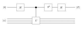
The QAS algorithm involves three steps (see Fig.1 for pictorial synopsis).
-
1.
Ansatz selection
-
2.
Calculation of the overlap matrices on a quantum computer
-
3.
Solving the differential equation using equations 15 on a classical computer
The first step of the QAS algorithm is crucial and heavily determines the accuracy of the algorithm. We consider our Ansatz to be a linear combination of cumulative -moment states, i.e.,
| (17) |
where For the given selection of the Ansatz in Eq.17, the second step of the QAS algorithm involves computing the overlap matrices. The matrix elements of can be estimated efficiently on a quantum computer, using the techniques from Mitarai et al., without any complicated measurement such as the Hadamard test Mitarai and Fujii (2019). If the Hamiltonian is a linear combination of tensored Pauli operators, the elements can be directly inferred from measurements in the corresponding computational basis as we further discuss later on as well as in Appendix E. Once the overlap matrices have been computed, the job of the quantum computer is over. For the third and final step of the QAS algorithm we solve Eq. 15 on a classical computer. If the desired accuracy has not been attained, one can re-run the whole algorithm for an increased choice of .
III Justification for the Ansatz
We now proceed to provide a small justification for the choice of the Ansatz in the QAS algorithm. Suppose the initial state (-moment state) is . Starting with , if one applies for some , the evolved state is given by
| (18) |
Using , we get
| (19) |
Let us define the operator
| (20) |
for Notice that corresponds to the sum of first terms of Using we proceed to define
| (21) |
For , Using the expression for Hamiltonian as linear combination of unitary, it is easy to see that can be written as linear combination of cumulative -moment states, i.e,
where the combination coefficients The aforementioned arguments justify the choice of Ansatz as linear combination of cumulative -moment states. Our Ansatz is based on the Krylov subspace idea. For a scalar , a matrix and a -dimensional vector , the action of the matrix exponential operator on can be approximated as Lanczos (1950); Saad (1992); Seki and Yunoki (2021); Motta et al. (2020)
| (22) |
where is a degree polynomial. The approximation in Eq.(22) is an element of the Krylov subspace,
| (23) |
Thus, the problem of approximating can be recast as finding an element from Note that the approximation in Eq.(22) becomes exact when In our case, we can identify with the initial state , with and with the Hamiltonian . Thus, one could implement the Krylov subspace ansatz directly with QAS by using the ansatz space . However, here we would have to estimate overlaps involving , which is a challenge for NISQ computers. Importance sampling has been proposed to estimate McClean et al. (2020), however this may require more measurements than current NISQ computers can handle. Our cumulative -moment states as shown in Definition 1 subsumes the Krylov subspace, however in contrast can be measured in a NISQ friendly way as we show below.
QAS requires the measurement of overlaps. For commonly used Hamiltonians, the unitaries in Eq.(2) are Pauli strings , where . In this case, the overlaps can be easily measured on NISQ devices. The matrix elements of and (Eqs.9,11) are written as , which can be rewritten as a single Pauli string with a prefactor . Thus, the measurement of overlaps simply becomes the measurement of Pauli strings, which is efficient on current NISQ devices via a simple sampling task. We discuss further details on measurements of overlaps in the Appendix E.
IV Examples
We now show examples of the QAS algorithm applied to various Hamiltonians and Ansatz states. First, in Fig.2, we investigate two elementary examples. In Fig.2a, we show the evolution with QAS of a single qubit for the Hamiltonian . In step of the QAS algorithm, we choose the initial Ansatz state (-moment state) . Then, following Definition 1, we use the set of unitaries that make up the Hamiltonian and generate the -moment states with . The union of and gives us the cumulative -moment states . Higher orders of the moment expansion can be prepared by repeating this approach. In step 2, we calculate the overlap matrices , (Eq.9, 11). Then, in step , we choose initial state of evolution with and , and then evolve to get the superposition state . We show the evolution of the expectation value of the Pauli operator . We find that the simulation with QAS and the exact evolution matches for the first moment expansion () as the set of -moment states closes here already.
Next, in Fig.2b, our initial state for evolution is a deep quantum circuit as studied in McClean et al. (2018) to demonstrate the so-called barren plateau problem of variational quantum algorithms. This Ansatz consists of qubits with layers of unitaries, composed of alternating single-qubit rotations around randomly chosen -, - or -axis parameterized with parameter and control phase gates arranged in a hardware efficient manner. This circuit suffers from the barren plateau problem where the variance of the gradients of the circuit in respect to an underlying cost function vanishes exponentially with the number of qubits , i.e. . For variational quantum algorithms, evolving these states is difficult as the gradients become exponentially small with increasing . While optimizing the circuit parameters is difficult, we show that we can simulate quantum dynamics with the very same state by using our QAS method instead. As QAS does not adjust the parameters , and instead only varies the classical parameter of the linear combination of states ansatz, we can circumvent the barren plateau problem. We now evolve this deep circuit as initial state with the Hamiltonian as chosen by Ref.McClean et al. (2018). We measure the overlaps Eqs.(11),(9) and solve Eq.(15). We find that we can already reproduce the time evolution of this state for the first moment expansion .
 a
a  b
b


Next, we discuss two further examples for the same variational Ansatz for different Hamiltonians in Fig.3. We evolve in Fig.3a this Ansatz with the Hamiltonian . After applying the Jordan-Wigner transformation Jordan and Wigner (1993), this Hamiltonian corresponds to a system of fermions tunneling from the first to the last site in a lattice system of length with , where () is the fermionic creation (annihilation) operator acting on site . Evolving this Hamiltonian with naive implementations of Trotter can be difficult as it requires implementing a -qubit rotation. We show fidelity of QAS with the exact evolution . We find optimal fidelity for moment . In Fig.3b we show the evolution of an exemplary many-body Hamiltonian, the Ising model. The Hamiltonian is given by
| (24) |
which describes a spin system with nearest-neighbor coupled spins with amplitude and an applied transverse magnetic field . We find increasing fidelity with increasing . For , the -moment states cover the full dynamics of the problem and thus we achieve unit fidelity.
 a
a  b
b


Now, we discuss QAS for dynamical simulation of a chemistry problem. In Fig.4, we show the evolution of an excited state of a LiH molecule. The LiH molecule Hamiltonian is mapped to 6 qubits using STO-3G basis using methods of McArdle et al. (2020), resulting in a Hamiltonian with 174 terms. We find that for the moment, the dynamics can be fully reproduced with QAS.


In Fig.5, we evolve a many-body Hamiltonian that consists of randomly chosen -body Pauli strings , where . The cumulative -moment states capture at order the full dynamics. We can simulate the dynamics for thousands of qubits . We show the simulation of the dynamics of an initial product state using a classical computer. For a general entangled initial state, the overlaps required for QAS are intractable for classical computers and one requires a quantum computer to simulate the dynamics.
Finally, we discuss imaginary time evolution with QAS. We defer the details to Appendix C. In Fig.6, we show the energy of the imaginary time evolution of the Ising model for the deep variational Ansatz introduced above. With longer evolution time, the energy of the quantum state decreases, until it reaches a minimal value. The found minimal energy decreases with increasing , reaching the exact ground state for .


We show further examples for the simulated dynamics for a quenched many-body system in Appendix D.
V Discussion and Conclusion
In this work, we provided a hybrid quantum-classical algorithm for simulating the dynamical evolution of a quantum system. Without loss of generality, we assume the Hamiltonian to be a linear combination of unitaries. Our algorithm proceeds in three steps and does not mandate any classical-quantum feedback loop. For algorithms with feedback loops, the quantum computer has to wait until the classical computer has executed its task. Most of the currently available quantum computers are accessed in a queue fashion and the feedback loop yields the whole process extremely slow, as the waiting time in the queue can be a few hours. The absence of the feedback loop renders our protocol exceptionally faster than its variational alternatives. The first step of the algorithm involves the selection of the Ansatz. We consider our Ansatz to be a linear combination of quantum states, where the quantum states belong to the set of cumulative -moment states, constructed using the unitaries defining the Hamiltonian. The combination coefficients are complex numbers in general. For the choice of the Ansatz in the first step, the second step involves the computation of two overlap matrices on the quantum computer. This step can be performed efficiently on existing quantum computers without the requirement of any complicated measurements by measuring Pauli strings. Once the overlap matrices have been computed, the third (and final) step of the QAS algorithm involves solving the differential equation and updating the parameters corresponding to Eq. (15) and (16) on a classical computer. If the desired accuracy has not been attained, one can re-run the whole algorithm for a different choice of .
It is in general difficult for classical computers to calculate quantum states. Here, the advantage of our algorithm comes into play. With a quantum computer, we can prepare quantum states out of reach for classical computers. Then, we measure overlaps via sampling from the quantum computers, which is in general a difficult task for classical computers, including tensor network methods. Above statement is bolstered by the Quantum Threshold Assumption (QUATH) Aaronson and Chen (2016) by Aaronson and Chen. It states that there is no polynomial-time classical algorithm which takes as input a random circuit and can decide with success probability at least that whether is greater than the median of taken over all bitstrings . Finally, the task of integrating the time evolution using the overlaps is left to the classical computer, as this task can be efficiently performed there. Our algorithm solves the task of quantum simulation by leaving classically easy tasks to the classical computer, and distributing only the classically difficult tasks to the quantum computer. This way, we use the resources available in the NISQ era prudently.
Apart from Dirac and Frenkel variational principle, there are two other variational principles, which can be used for variational simulation of dynamics: the McLachlan variational principle McLachlan (1964) and the time-dependent variational method principle Kramer and Saraceno (1980); Broeckhove et al. (1988). For an Ansatz with complex adjustable parameters, all three variational principles lead to same dynamical evolution Yuan et al. (2019). We also discussed the extension of our algorithm to imaginary time evolution (see Appendix C for details). It is noteworthy to stress that the quantum states defining the Ansatz are fixed, and only the variational parameters are (classically) updated. The algorithm does not mandate the computation of gradients using the quantum computer and thus circumvents the barren plateau problem by construction. Our approach of linear combination of quantum states could offer an advantage even at the level of initial state preparation. There exists cases where the initial state is difficult to prepare, but is respresentable as linear combination of -moment states for some efficiently preparable zero-moment state. Such cases though intractable via variational algorithms such as VQS, are easily simulable with our method. Our algorithm can easily subsume VQS using the following Ansatz
| (25) |
where and
Since we unlock a fresh paradigm, there are many open questions for further investigation. In future, one could study the extension of our algorithm for simulating open system dynamics, in the presence of noise as well as for Gibbs state preparation. Extending our algorithm to simulate generalized time evolution is another exciting direction Endo et al. (2020). It would be interesting to provide complexity-theoretic guarantees as well as analyze the error in-depth. A proper study of the Ansatz construction is another exciting direction. We believe that an in-depth study of our algorithm will lead to the design of quantum-inspired classical algorithms for simulating the dynamics of quantum systems.
Acknowledgements.
We are grateful to the National Research Foundation and the Ministry of Education, Singapore for financial support. We thank Jonathan for interesting discussions.References
- Preskill (2018) J. Preskill, Quantum 2, 79 (2018).
- Deutsch (2020) I. H. Deutsch, arXiv preprint arXiv:2010.10283 (2020).
- Bharti et al. (2021) K. Bharti, A. Cervera-Lierta, T. H. Kyaw, T. Haug, S. Alperin-Lea, A. Anand, M. Degroote, H. Heimonen, J. S. Kottmann, T. Menke, W.-K. Mok, S. Sim, L.-C. Kwek, and A. Aspuru-Guzik, arXiv:2101.08448 (2021).
- Arute et al. (2019) F. Arute, K. Arya, R. Babbush, D. Bacon, J. C. Bardin, R. Barends, R. Biswas, S. Boixo, F. G. Brandao, D. A. Buell, et al., Nature 574, 505 (2019).
- Peruzzo et al. (2014) A. Peruzzo, J. McClean, P. Shadbolt, M.-H. Yung, X.-Q. Zhou, P. J. Love, A. Aspuru-Guzik, and J. L. Obrien, Nature communications 5, 4213 (2014).
- McClean et al. (2016) J. R. McClean, J. Romero, R. Babbush, and A. Aspuru-Guzik, New Journal of Physics 18, 023023 (2016).
- Kandala et al. (2017) A. Kandala, A. Mezzacapo, K. Temme, M. Takita, M. Brink, J. M. Chow, and J. M. Gambetta, Nature 549, 242 (2017).
- Farhi et al. (2014) E. Farhi, J. Goldstone, and S. Gutmann, arXiv:1411.4028 (2014).
- Farhi and Harrow (2016) E. Farhi and A. W. Harrow, arXiv preprint arXiv:1602.07674 (2016).
- Harrow and Montanaro (2017) A. W. Harrow and A. Montanaro, Nature 549, 203 (2017).
- McArdle et al. (2020) S. McArdle, S. Endo, A. Aspuru-Guzik, S. C. Benjamin, and X. Yuan, Reviews of Modern Physics 92, 015003 (2020).
- Endo et al. (2021) S. Endo, Z. Cai, S. C. Benjamin, and X. Yuan, Journal of the Physical Society of Japan 90, 032001 (2021).
- Bittel and Kliesch (2021) L. Bittel and M. Kliesch, arXiv:2101.07267 (2021).
- McClean et al. (2018) J. R. McClean, S. Boixo, V. N. Smelyanskiy, R. Babbush, and H. Neven, Nature communications 9, 4812 (2018).
- Huang et al. (2019) H.-Y. Huang, K. Bharti, and P. Rebentrost, arXiv preprint arXiv:1909.07344 (2019).
- Sharma et al. (2020) K. Sharma, M. Cerezo, L. Cincio, and P. J. Coles, arXiv preprint arXiv:2005.12458 (2020).
- Cerezo et al. (2020) M. Cerezo, A. Sone, T. Volkoff, L. Cincio, and P. J. Coles, arXiv preprint arXiv:2001.00550 (2020).
- Wang et al. (2020) S. Wang, E. Fontana, M. Cerezo, K. Sharma, A. Sone, L. Cincio, and P. J. Coles, arXiv preprint arXiv:2007.14384 (2020).
- Marrero et al. (2020) C. O. Marrero, M. Kieferová, and N. Wiebe, arXiv preprint arXiv:2010.15968 (2020).
- Bharti (2020) K. Bharti, arXiv preprint arXiv:2009.11001 (2020).
- Bharti and Haug (2020) K. Bharti and T. Haug, arXiv preprint arXiv:2010.05638 (2020).
- Poulin et al. (2014) D. Poulin, M. B. Hastings, D. Wecker, N. Wiebe, A. C. Doherty, and M. Troyer, arXiv:1406.4920 (2014).
- Li and Benjamin (2017) Y. Li and S. C. Benjamin, Physical Review X 7, 021050 (2017).
- McArdle et al. (2019) S. McArdle, T. Jones, S. Endo, Y. Li, S. C. Benjamin, and X. Yuan, npj Quantum Information 5, 1 (2019).
- Yuan et al. (2019) X. Yuan, S. Endo, Q. Zhao, Y. Li, and S. C. Benjamin, Quantum 3, 191 (2019).
- Dirac (1930) P. A. Dirac, in Mathematical Proceedings of the Cambridge Philosophical Society, Vol. 26 (Cambridge University Press, 1930) pp. 376–385.
- Frenkel et al. (1934) I. Frenkel et al., (1934).
- Mitarai and Fujii (2019) K. Mitarai and K. Fujii, Physical Review Research 1, 013006 (2019).
- Lanczos (1950) C. Lanczos, (1950).
- Saad (1992) Y. Saad, SIAM Journal on Numerical Analysis 29, 209 (1992).
- Seki and Yunoki (2021) K. Seki and S. Yunoki, PRX Quantum 2, 010333 (2021).
- Motta et al. (2020) M. Motta, C. Sun, A. T. Tan, M. J. O’Rourke, E. Ye, A. J. Minnich, F. G. Brandão, and G. K.-L. Chan, Nature Physics 16, 205 (2020).
- McClean et al. (2020) J. R. McClean, Z. Jiang, N. C. Rubin, R. Babbush, and H. Neven, Nature communications 11, 1 (2020).
- Jordan and Wigner (1993) P. Jordan and E. P. Wigner, in The Collected Works of Eugene Paul Wigner (Springer, 1993) pp. 109–129.
- Aaronson and Chen (2016) S. Aaronson and L. Chen, arXiv preprint arXiv:1612.05903 (2016).
- McLachlan (1964) A. McLachlan, Molecular Physics 8, 39 (1964).
- Kramer and Saraceno (1980) P. Kramer and M. Saraceno, in Group Theoretical Methods in Physics (Springer, 1980) pp. 112–121.
- Broeckhove et al. (1988) J. Broeckhove, L. Lathouwers, E. Kesteloot, and P. Van Leuven, Chemical physics letters 149, 547 (1988).
- Endo et al. (2020) S. Endo, J. Sun, Y. Li, S. C. Benjamin, and X. Yuan, Phys. Rev. Lett. 125, 010501 (2020).
Appendix A Error Analysis
Appendix B Realification
Recall that the Ansatz evolution equation is given by
| (28) |
where . Moreover, the overlap matrices and can be in general complex. We can use realification to solve the above differential equation for . The idea of realification is to create a mapping from to The crux of the idea is the following real matrix representation for and ,
| (29) |
and
| (30) |
It can be seen that which mimics Let , and , be the real and imaginary parts of the overlap matrices and Let and be the real and imaginary parts of Using the mappings in 29 and 30, one can obtain the following representation for
| (31) |
| (32) |
and
| (33) |
Using the above representation, one trivially gets the following realified evolution equation.
| (34) |
Appendix C Imaginary Time Evolution
Substituting with in the Schrödinger equation we get
| (35) |
where The presence of preserves the norm of Let us consider the Ansatz state as linear combination of quantum states
| (36) |
for Using Dirac and Frenkel variational principle, we get
| (37) |
where
| (38) |
The evolution of parameters is given by
| (39) |
where and are
| (40) |
| (41) |
Further simplification leads to
| (42) |
Appendix D Quantum Quench
We now give further numerical examples for QAS. We demonstrate quench dynamics for many-body systems. Here, the system is prepared in the ground state of a Hamiltonian. Then, to generate the dynamics, the parameters of the Hamiltonian are instantaneously changed to another value. We show two examples for such dynamics in Fig.7. We study the Ising Hamiltonian given by
| (43) |
and the Heisenberg model
| (44) |
which describe spin systems with nearest-neighbor coupled spins with parameters and . We find that for the Ising Hamiltonian (Fig.7a), the evolution becomes more accurate with increasing , reaching optimal fidelity for . In Fig.7b, we study the Heisenberg model. We find that we converge to optimal fidelity for .
 a
a  b
b


Appendix E Measurements
We reiterate here the content from reference Bharti and Haug (2020). For the purposes of this section, a unitary will be referred -local if it acts non-trivially on at most qubits. We assume . The moment- Ansatz, for some positive integer , in QAS algorithm requires computation of matrix elements of the form where is a k-local unitary matrix (since is product of at most k-local unitary matrices). By invoking the following result from Mitarai et. al. Mitarai and Fujii (2019), we guarantee an efficient computation of the overlap matrices on a quantum computer without the use of the Hadamard test.
Fact 2.
Mitarai and Fujii (2019) Let k be an integer such that , where is the number of qubits and be an -qubit quantum state. For any k-local quantum gate it is possible to estimate up to precision in time without the use of the Hadamard test, with classical preprocessing of time
We proceed to discuss the methodology suggested in (Mitarai and Fujii, 2019) to calculate the required matrix elements. For detailed analysis, refer to (Mitarai and Fujii, 2019). Since is a -local unitary, it can be decomposed as such that acts on qubits. Clearly, is a matrix. Suppose the eigenvalues of are Using the integers let us denote the computational basis of each subsystem by We diagonalize each and obtain some unitary matrix such that where Since , the aforementioned diagonalized can be performed in polynomial time. A simple calculation gives,
| (45) |
Thus, one can evaluate by calculating the probability of getting from the measurement of in the computational basis.
If the unitaries defining the Hamiltonian are Pauli strings over qubits, one can use the following Lemma Huang et al. (2019) to provide an estimate of the number of measurements needed to achieve a given desired accuracy.
Lemma 3.
Huang et al. (2019) Let and be a Pauli string over qubits. Let multiple copies of an arbitrary -qubit quantum state be given. The expectation value can be determined to additive accuracy with failure probability at most using copies of
We now discuss how to measure the matrix elements of and for the special case where the components of the Hamiltonian are Pauli strings , with . For a -moment state expansion of Ansatz , the elements to calculate are
| (46) |
Now, each overlap element is a product of a set of some Pauli strings to be measured on state , with . The product rule of Pauli operators states that , where , is the Kronecker delta and the Levi-Civita symbol. Thus, a product of two Pauli strings is again a Pauli string , with a prefactor . To calculate the matrix elements on the quantum computer, first one has to evaluate which Pauli string corresponds to the product of unitaries in Eq.46 and the corresponding prefactor. Then, the expectation value of the resulting Pauli string is measured for the Ansatz state . This observable is a hermitian operator, and can be easily measured by rotating each qubit into the computational basis corresponding to the Pauli operator. Finally, the expectation value of the measurement is multiplied with the prefactor .