Identifying Majorana bound states by tunneling shot-noise tomography

Abstract

Majorana fermions are promising building blocks of forthcoming technology in quantum computing. However, their non-ambiguous identification has remained a difficult issue because of the concomitant competition with other topologically trivial fermionic states, which poison their detection in most spectroscopic probes. By employing numerical and analytical methods, here we show that the Fano factor tomography is a key distinctive feature of a Majorana bound state, displaying a spatially constant Poissonian value equal to one. In contrast, the Fano factor of other trivial fermionic states, like the Yu-Shiba-Rusinov or Andreev ones, is strongly spatially dependent and exceeds one as a direct consequence of the local particle-hole symmetry breaking.

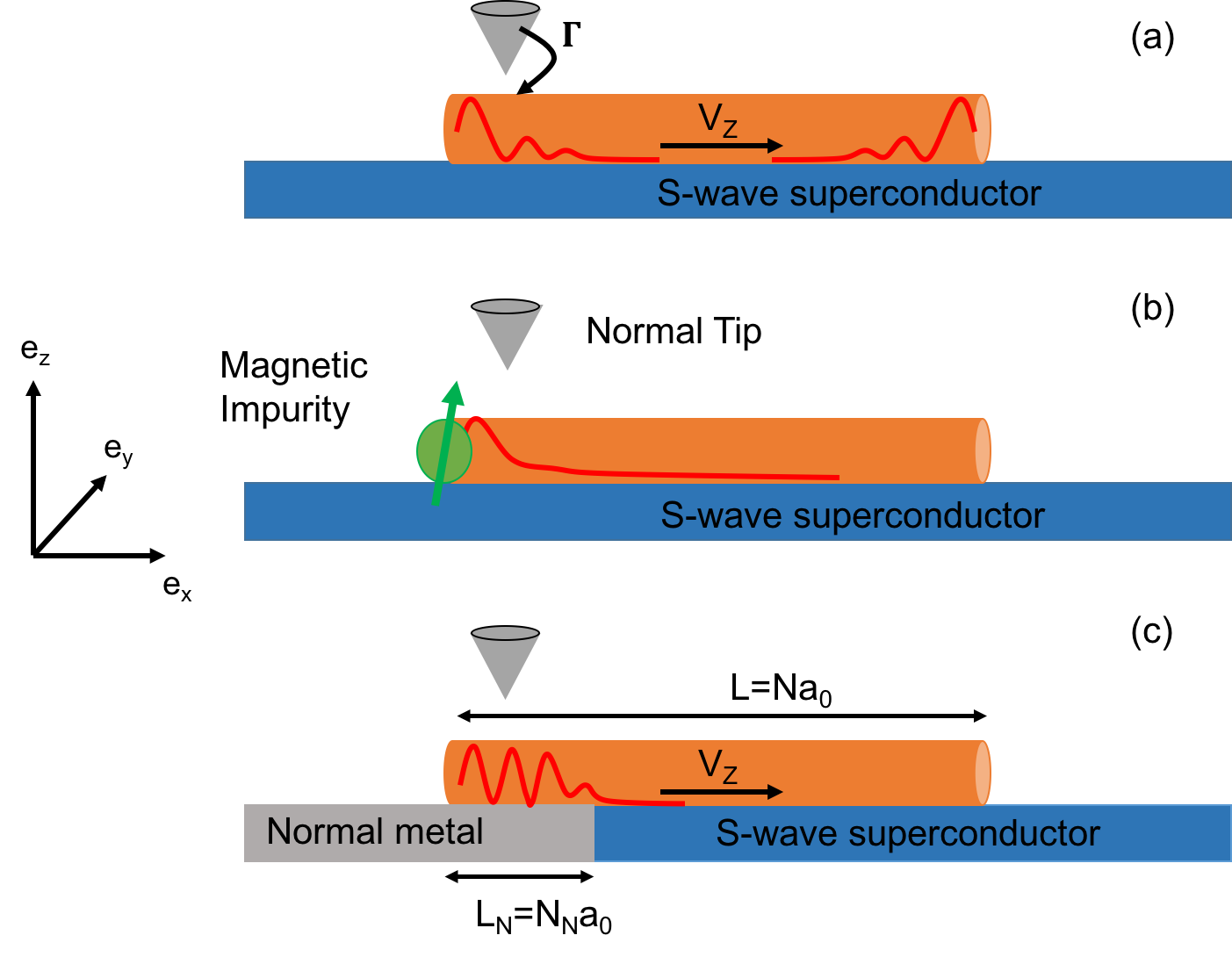
Figure 1: Schematic representation of the typical experimental set-up considered. (a) A nano-wire placed on top of a s-wave superconductor subject to an external Zeeman field $V_{Z}$ along the wire $\mathbf{e}_{x}$ axis. This system can host MBS at its ends, as depicted by the red solid lines. (b) A nano-wire terminated by a magnetic impurity on top of a s-wave superconductor. This system hosts a YSR bound-state at its left-end (red solid line). (c) Same as in a) except that the substrate contains a small normal region. This system can host ABS (red solid lines). In all cases, the wire is probed by a metallic tip via tunneling effect of strength $\Gamma$.

Since the theoretical work of Kitaev Kitaev (2001) the search of Majorana bound-states (MBS) has been a highly investigated topic in condensed matter. MBS are promising building blocks for quantum information processing Alicea (2010) because they are protected from local perturbation and possess non-Abelian braiding statistics. Many platforms exhibiting MBS have been experimentally studied in the past decade. This includes semiconducting wires in proximity of a s-wave superconductor Lutchyn et al. (2018), vortices in iron-based superconductors Wang et al. (2018); Chiu et al. (2020), two-dimensional (2D) phase-controlled Josephson junctions Ren et al. (2019); Fornieri et al. (2019), and one-dimensional (1D) chains of magnetic atoms on top of a superconducting substrate Nadj-Perge et al. (2014); Ruby et al. (2015); Pawlak et al. (2016); Feldman et al. (2017); Kim et al. (2018), to list a few.

Recent scanning tunneling spectroscopy (STS) on self-assembled magnetic chains or magnetic atoms on a s-wave superconducting surface have revealed the existence of zero bias peaks, spatially localized at the end of such chains Nadj-Perge et al. (2014); Ruby et al. (2015); Pawlak et al. (2016); Feldman et al. (2017); Kim et al. (2018). These measurements have been interpreted as signatures of topologically protected MBS. However this conclusion remains openly debated. Indeed, zero-bias peaks could also be due to the presence of other trivial zero-energy fermionic bound states mimicking topologically protected MBS Ruby et al. (2015), like, e.g., Yu-Shiba-Rusinov (YSR) bound states Balatsky et al. (2006), Andreev bound states (ABS) and quasi-Majorana states (QMS) Kells et al. (2012); Prada et al. (2012); Liu et al. (2017); Moore et al. (2018); Vuik et al. (2019); Rossi et al. (2020); Prada et al. (2020).

Therefore, having clear experimental protocols capable to distinguish trivial fermionic bound-states from MBS is highly desirable. In this respect, conductance tomography has been proposed as a promising route, as the zero-bias conductance peak due to a pure MBS is quantized. Such a quantization is however weak against quasiparticle poisoning Peng et al. (2015a); Das Sarma and Pan (2021) or inhomogeneities of the superconducting order parameter Fleckenstein et al. (2018) and moreover necessitates a strong tunneling regime to observe a distinctive conductance saturation-plateau in proximity of MBS Chevallier and Klinovaja (2016).

Following earlier theoretical predictions about non-trivial spin signatures of MBS Sticlet et al. (2012); Haim et al. (2015); Björnson et al. (2015); Kotetes et al. (2015); Setiawan et al. (2015); Szumniak et al. (2017) and spin-selective Andreev reflection He et al. (2014); Sun et al. (2016), Jeon et al. have used spin polarized STS as a diagnostic tool Jeon et al. (2017). However, discerning some local excess of polarization over a magnetic background remains a difficult task. Other possible signatures of MBS could be provided by current shot-noise Law et al. (2009), spin-resolved shot-noise measurements Haim et al. (2015); Devillard et al. (2017), finite-frequency current shot-noise Jonckheere et al. (2020), or time-resolved transport spectroscopy Tuovinen et al. (2019). However, such protocols are more involved than the ones employed in usual STS.

Here we focus on the most typical MBS experimental set-up, the hybrid magnetic-superconducting wire. We show that the current shot-noise spatial tomography with a metallic tip, nowadays realized within scanning tunneling microscopy (STM) Massee et al. (2018); Bastiaans et al. (2018), can distinguish MBS from other zero-energy fermionic states. In particular, we shall prove that the MBS Fano factor is spatially constant and equals to one, the Poissonian limit. This result is a consequence of the local particle-hole symmetry of the MBS wave function. However, in other zero-energy trivial bound states, like YSR or ABS, the breaking of such a symmetry implies a strongly spatially dependent Fano factor. Even for the case of QMS, we shall show that the Fano factor oscillates above 1 in the superconducting part of the wire. Although our proposal cannot definitely distinguish whether MBS are topologically protected Prada et al. (2020), the spatially unity Fano factor is a clear distinguishing signature of the Majorana wave function.

Models and methods. The typical system that we consider consists of a nanowire deposited on a conventional s-wave superconductor Lutchyn et al. (2010); Oreg et al. (2010) [see Fig. 1(a)] in presence of spin orbit interactions (SOI) and a Zeeman field. We first study a zero-energy YSR state created by a magnetic impurity located at one extremity of the wire [as depicted in Fig. 1(b)]. As second reference case, we study ABS which can be obtained by assuming the $N_{N}$ first sites of the wire in contact with a normal substrate [Fig. 1(c)]. This situation can also harbor a QMS by fine-tuning a confining potential separating the normal and superconducting part.

A tight-binding Bogoliubov-de Gennes (BdG) Hamiltonian describing such configuration reads

$$\mathcal{H}_{S}= \frac{1}{2}\sum_{l=0}^{N-1}\psi^{\dagger}_{l,S}[(2t-\mu+V(l))\tau_{z}+\Delta(l)\tau_{x}+V_{Z}\sigma_{x}]\psi_{l,S}$$

$$+\frac{1}{2}\sum_{l=0}^{N-2}\psi^{\dagger}_{l+1,S}[-{t_{w}}\tau_{z}-i\alpha\sigma_{y}\tau_{z}]\psi_{l,S}+\text{H.c.}$$

$$-\frac{1}{2}\psi^{\dagger}_{0,S}J\sigma_{z}\psi_{0,S}~{},$$ (1)

where $N$ is the total number of chain sites. Here we define the Nambu-spinor $\psi_{l,S}=(c_{\uparrow,l},c_{\downarrow,l},c^{\dagger}_{\downarrow,l},-c^{\dagger}_{\uparrow,l})^{T}$, where the operator $c_{\sigma,l}$ annihilates an electron of spin $\sigma$ at site $l$ of the nanowire. $\Delta(l)=\Delta\,\Theta({l+1-N_{N}})$ represents a non-uniform pairing potential induced by proximity effect with the superconducting substrate, $\Theta({l+1-N_{N}})$ is the Heaviside step function and $N_{N}$ is the size of the normal region of the wire. $V(l)=V_{0}\exp(-\frac{(l-N_{N})^{2}}{2\sigma^{2}})$ is a smooth Gaussian potential barrier at the NS interface. The Pauli matrices $\tau_{i}$ and $\sigma_{i}$ act in the particle-hole and spin spaces respectively, $\mu$ denotes the chemical potential, $t_{w}$ the nearest-neighbor hopping, $V_{Z}$ the Zeeman exchange energy, $\alpha$ the SOI. Finally, $J$ is the local exchange coupling due to a magnetic atom localized on the left end of the wire (Fig. 1b). This model is rather general, but we shall focus on 6 experimentally relevant cases Chevallier and Klinovaja (2016); Haim et al. (2015); Vuik et al. (2019), described in Table I. For $N_{N}=0$, the whole wire is superconducting. When $J=0$ and $V_{Z}>\sqrt{\mu^{2}+\Delta_{0}^{2}}$, (case a), a topological phase characterized by MBS at the ends of the wire emerges (Fig. 1a) Lutchyn et al. (2010); Oreg et al. (2010). When $J\neq 0$, (case b), a YSR bound state appears on the wire left end [Fig. 1(b)]. For $N_{N}>0$, the left part of the wire is in normal state. In this case, when $V_{Z}>\sqrt{\mu^{2}+\Delta_{0}^{2}}$, (case c), MBS are present while for $V_{Z}<\sqrt{\mu^{2}+\Delta_{0}^{2}}$ a trivial zero-energy ABS localized in the normal region can appear due to fine tuning of parameters. Finally, when $V_{Z}>\sqrt{\mu^{2}+\Delta_{0}^{2}}$ and a smooth potential barrier is present at the NS interface (case e), MBS are present while for $V_{Z}<\sqrt{\mu^{2}+\Delta_{0}^{2}}$, a zero-energy QMS can appear due to the smooth confinement potential (case f) Vuik et al. (2019); Prada et al. (2020); Sup . Note that this Hamiltonian is also suitable to describe a ferromagnetic nanowire grown on a substrate with strong SOI. This situation occurs, e.g., in Pb Nadj-Perge et al. (2014); Ruby et al. (2015); Pawlak et al. (2016) or in an array of magnetic impurities adsorbed on a superconducting substrate Kim et al. (2018) displaying a helical magnetic ground state Choy et al. (2011); Nadj-Perge et al. (2013); Braunecker and Simon (2013); Klinovaja et al. (2013); Vazifeh and Franz (2013); Pientka et al. (2013, 2014); Pöyhönen et al. (2014); Westström et al. (2015); Peng et al. (2015b); Hui et al. (2015); Braunecker and Simon (2015). In such a situation $V_{Z}$ describes the magnetic exchange energy.

	Case	$\mu$	$t_{w}$	$\Delta$	$V_{Z}$	$\alpha$	$J$	$N$	$N_{N}$	$V_{0}$	$s$	$\Delta_{\rm eff}$
a	MBS 1	0.5	10	1	2	1.2	0	80	0	0	X	0.63
b	YSR	0.5	10	0.6	0	1.2	11.23	80	0	0	X	0.6
c	MBS 2	0.5	10	1	1.4	2	0	100	20	0	X	0.31
d	ABS	0.5	10	1	0.38	2	0	100	20	0	X	0.27
e	MBS 3	1	10	2	3.2	3	0	100	20	4.5	5	0.27
f	QMS	3	10	1	2.75	3	0	100	20	4.5	5	0.27

Table 1: Table summarizing 6 different parameter sets of experimentally relevant situations. $\Delta_{\rm eff}$ is the effective gap separating the zero-energy bound-state from other states.

In all cases summarized in Table I, zero energy bound states do appear well separated from other states by a gap $\Delta_{\rm eff}$. This can be visualized in the single-particle density of states plotted in the insets of Fig. 2.

In the customary weak tunneling regime, STM allows to detect the local density of states (LDoS) $\rho(j,\omega)$. However, the LDoS does not allow for a clear distinction between trivial states and MBS, because of interference or other non-universal effects Sup . These complications could be overcome in the strong tunneling regime, which is dominated by Andreev reflections as recently shown experimentally Ruby et al. (2015). In that case, it is expected that the differential conductance in the vicinity of MBS is quantized, displaying a flat spatial profile Peng et al. (2015a). However, the oscillations of the MBS wave function ultimately spoil the conductance plateau and do not allow once again to discriminate MBS from trivial bound states Chevallier and Klinovaja (2016). In what follows, we show that, within a rather strong tunneling regime, shot-noise STM is the right observable that allows such discrimination.

To model the STM experiment we define the complete Hamiltonian $\mathcal{H}_{tot}=\mathcal{H}_{T}+\mathcal{H}_{S}+\mathcal{H}_{tunnel},$ which includes the coupling between the tip and the sample:

$$\mathcal{H}_{tunnel} =\frac{t}{2}[\psi^{\dagger}_{T}\tau_{z}\psi_{j,S}]+\text{H.c.}.$$ (2)

Here we introduce the Nambu-spinor $\psi_{T}=(d_{\uparrow},d_{\downarrow},d^{\dagger}_{\downarrow,},-d^{\dagger}_{\uparrow})^{T}$, where the operator $d_{\sigma}$ annihilates an electron of spin $\sigma$ at the apex of the tip. $\mathcal{H}_{T}$ is the Hamiltonian of the isolated metallic tip and $\mathcal{H}_{tunnel}$ describes the sample-tip tunneling, which is assumed purely local. We fix $\hbar=1$ throughout. Tunneling events are thus characterized by the energy width $\Gamma=2\pi\nu_{T}t^{2}$, where $\nu_{T}$ is the density of states in the tip. The bias voltage $V$ between the tip and the sample is taken into account in the chemical potential of the tip as $\mu_{T}=\mu+eV$.

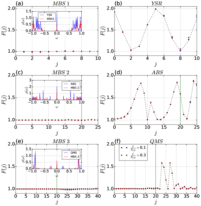
Figure 2: Dots: Fano factor as a function of the tip position ($j$) at fixed voltage $eV=0.7\Delta_{\rm eff}$ for increasing tunneling strengths ($\Gamma/\Delta_{\rm eff}=0.1,0.3$) for different zero-energy states: MBS 1 (a), YSR (b), MBS 2 (c), ABS (d), MBS 3 (e), and QMS (f) (see Table I). In the vicinity of MBS, cases (a),(c) and (e), a flat plateau $F(j)=1$ is observed in sharp contrast with trivial cases (b) and (d) where strong oscillations of $F$ well above $1$ are obtained. In vicinity of a QMS, case (f), $F(j)=1$ in the whole metallic region, where the Majorana wavefunctions do not overlap, however as they start overlapping in the SC region, $20<j<40$, (see Sup ) spatial oscillations of $F$ above 1 are found, allowing for a distinction with the isolated MBS of case (e). Dashed line: Analytical approximation obtained from the low-energy models Eq. (8) and Eq. (9). The low-energy approximation is in excellent agreement with numerical points. The green line denotes the NS interface when it exists. The three insets show the DOS for the six cases considered here.

Current shot-noise. The charge current flowing from the tip is $I(j,t_{1})=-e\frac{d\hat{N}_{T}(t_{1})}{dt_{1}}$, where $\hat{N}_{T}(t_{1})$ is the number operator counting the electrons in the tip at time $t_{1}$ in the Heisenberg picture. In the dc regime, $I(j,t_{1})=I(j)$ and

$$\langle I(j)\rangle=\frac{et}{2}\int\frac{d\omega}{2\pi}\Tr{G^{<}_{jS,T}(\omega)-G^{<}_{T,Sj}(\omega)},$$ (3)

where $G^{<}_{jS,T}(\omega)$ and $G^{<}_{T,Sj}(\omega)$ are local Keldysh Green’s matrices at site $j$, describing the electron hopping between the sample $S$ and the tip $T$. These and all the Green’s functions of the tip $G^{R/A}_{T,T}$, $G^{</>}_{T,T}$ and of the substrate $G^{R/A}_{jS,jS}$, $G^{</>}_{jS,jS}$ are related by equations of motion with the isolated tip $g^{R/A}_{T}$, $g^{</>}_{T}$ and isolated substrate $g^{R/A}_{S}$, $g^{</>}_{S}$ bare Green’s functions respectively Sup . The shot-noise is defined as the zero-frequency limit of the time-symmetrized current-current correlator, $S=\int d(t_{1}-t_{2})S(t_{1},t_{2})$, where $S(t_{1},t_{2})=\langle\delta I(t_{1})\delta I(t_{2})\rangle+\langle\delta I(t_{2})\delta I(t_{1})\rangle$ and $\delta I(t_{1})=I(t_{1})-\langle I(t_{1})\rangle$. Using the Wick theorem Sup , we find

$$S(j,eV)= {e^{2}t^{2}}\int\frac{d\omega}{2\pi}\Tr{G^{<}_{T,T}(\omega)G^{>}_{jS,jS}(\omega)}$$

$$- \Tr{G^{<}_{jS,T}(\omega)G^{>}_{jS,T}(\omega)}+(jS\leftrightarrow T).$$ (4)

Finally the Fano factor is given by

$$F(j,eV)=S(j,eV)/(2e|I(j,eV)|).$$ (5)

Consequently, with the retarded uncoupled Green’s functions $g^{R}_{T}$ and $g^{R}_{S}$ in hands, the charge current $I(j)$, the shot noise $S(j,eV)$ and the Fano factor $F(j,eV)$ are readily computed Sup .

Fano factor tomography (FFT). We numerically calculated the FFT of the wire for the different configurations displayed in Table I and many values of the tunneling amplitude. We shall present results for $\Gamma/\Delta_{\rm eff}=0.1,0.3$, which correspond to a strong tunneling strength. Typically, the shot-noise signal vanishes at low voltage (following the current) and rapidly saturates to finite value for higher voltage. We thus set $eV=0.7\Delta_{\rm eff}$, which assures that the signal has reached saturation. Since we are interested in the low-temperature quantum regime, we set $k_{B}T=\frac{\Delta_{\rm eff}}{200}$. We investigated temperature effects and our results showed that the FFT remains robust as long as $k_{B}T$ is much smaller than $\Delta_{\rm eff}$ Sup . Figures. 2()a, 2()c and 2(e) (which correspond to case a, c, and e, respectively, in Table I) show that the Fano factor in the vicinity of MBS states does not significantly deviate from the Poissonian limit, $F=1$ and does not depend strongly on the tip position ($j$). This behavior is observed for any tunneling regime. Notice that for the first sites of the wire ($j<5$) $F(j)$ weakly decreases to less than one when tunneling strength increases. In contrast, Fig. 2(b) (case b in Table I) shows that in vicinity of YSR bound-states, the Fano factor can reach values significantly greater than 1, oscillating strongly as a function of the tip position ($j$). This behavior is again observed for any tunneling regime and does not significantly depend on $\Gamma$. Those qualitative results are also found in the vicinity of an ABS, as plotted in Fig. 2d (case d in Table I). Our results for a QMS (case f) in Table I) are shown in Fig. 2f. This case is less discriminating as the Fano factor oscillates above 1 only in the superconducting part of the wire where the two Majorana wave functions start overlapping. In the following, we provide analytical insight into these results showing that they are universally rooted to the breaking of the particle-hole symmetry of unpaired MBS.
Insights from low-energy models. Within our BDG formalism applied to a one-band Hamiltonian, a general zero-energy state (topological or trivial) is associated to the 4 particle-hole component wave-function $\phi_{+}(j)=[u_{\uparrow}(j),u_{\downarrow}(j),v_{\uparrow}(j),-v_{\downarrow}(j)]^{T}$ and its particle-hole partner $\phi_{-}(j)=\sigma_{y}\tau_{y}\mathcal{K}\phi_{+}(j)$, where $\mathcal{K}$ denotes the complex conjugation. Using the Lehmann’s representation, and restricting to low-energy bound states, the sample retarded bare Green’s function reads $g^{R}_{S,j,j}(\omega)\approx\frac{\phi_{+}(j)\phi_{+}^{\dagger}(j)+\phi_{-}(j)\phi_{-}^{\dagger}(j)}{\omega+i0^{+}}.$ Under the general assumption that the sample Hamiltonian is real , $u_{\sigma}(j)$ and $v_{\sigma}(j)$ can be safely chosen as real numbers. By using the equations of motion Sup , we are able to obtain exact expressions for both the current and the shot-noise. In the general case of finite temperature and finite voltage, these expressions turn out to be lengthy and not insightful Sup . However, in the zero-temperature limit and saturated voltage regime, $eV\gg\Gamma_{j}$, with $\Gamma_{j}=\Gamma\sum_{\sigma}(|u_{\sigma}(j)|^{2}+|v_{\sigma}(j)|^{2})$, we obtain

$$S(j) \simeq{8e^{2}\Gamma}\frac{(\sum_{\sigma}u_{\sigma}^{2})(\sum_{\sigma}v_{\sigma}^{2})[(\sum_{\sigma}u_{\sigma}^{2})^{2}+(\sum_{\sigma}v_{\sigma}^{2})^{2}]}{(\sum_{\sigma}u_{\sigma}^{2}+\sum_{\sigma}v_{\sigma}^{2})^{3}},$$ (6)

$$I(j) \simeq{2e}\Gamma\frac{(\sum_{\sigma}u_{\sigma}^{2})(\sum_{\sigma}v_{\sigma}^{2})}{(\sum_{\sigma}u_{\sigma}^{2}+\sum_{\sigma}v_{\sigma}^{2})},$$ (7)

$$F(j) \simeq 1+\left(\frac{\sum_{\sigma}(u_{\sigma}^{2}-v_{\sigma}^{2})}{\sum_{\sigma}(u_{\sigma}^{2}+v_{\sigma}^{2})}\right)^{2}=1+\delta_{\rm ph}^{2}(j),$$ (8)

where $\delta_{\rm ph}(j)$ denotes the local particle-hole asymmetry. Consequently $F(j)$ does not depend on the tunneling strength and $1\leq F(j)$. Furthermore, and most importantly, we prove that $F(j)-1$ is in direct correspondence with $\delta_{\rm ph}(j)$ and can thus display strong spatial variations. Nonzero $\delta_{\rm ph}(j)$ obviously requires finite overlap of Majorana components, we thus expect $F$ to be sensitive to MBS overlap Sup . Indeed, we show in Figs. 2(b), 2(d) and 2(f) that the low-energy approximation of Eq. (8) is in excellent quantitative agreement with the numerical results.

In sharp contrast, a perfectly isolated MBS has a local particle-hole symmetry for any position, imposing strong constraints on the spatial dependence of $F(j)$. An isolated MBS is described by the retarded Green’s function, $g^{R}_{S,j,j}(\omega)=\frac{\phi_{M}(j)\phi_{M}^{\dagger}(j)}{\omega+i0^{+}}$ with $\phi_{M}(j)=(u_{\uparrow},u_{\downarrow},u_{\downarrow}^{*},-u_{\uparrow}^{*})^{T}$. Setting $T=0$, the shot-noise and current can be obtained exactly and have a compact form even for finite voltage. The resulting Fano factor reads

$$F(j,eV) =1-\frac{\Gamma_{j}}{\arctan(\frac{eV}{\Gamma_{j}})}\frac{eV}{(eV)^{2}+\Gamma_{j}^{2}}.$$ (9)

Therefore, in the saturated regime, $eV\gg\Gamma_{j}$, $F(j)\approx 1$ and the Fano factor does not depend on $j$. Moreover, the leading order corrections in $\frac{\Gamma_{j}}{eV}$ reads $F(j)\simeq 1-\frac{2\Gamma_{j}}{\pi eV}$, showing that the Fano factor in the vicinity of a MBS weakly decreases with increasing tunneling strength $\Gamma$ and takes values lower than 1, in agreement with the numerical curves displayed in Figs. 2(a), 2(c) and 2(e).

As any zero-energy Dirac fermions can be written as a pair of Majorana fermions Kitaev (2001), the breaking of the particle-hole symmetry, producing the large overshooting of the Fano factor above one, can be interpreted in terms of a spatial overlap of the two Majorana wavefunctions. This must be contrasted with the particle-hole symmetry preserved in a spatially well isolated MBS. We can directly prove this by analyzing how the Fano factor departs from $F\sim 1$ by increasing the overlap of the Majorana wavefunctions in the nanowire model (see Sup ). These arguments are general and rely only on the existence of a zero-energy bound state in an effective single-band Hamiltonian. Although the FFT does not provide any direct signature of the topology of the bulk substrate, it is of great practical interest to select those MBS, which do not overlap and are therefore resilient to local noise which makes them good candidates for quantum computation Prada et al. (2020).

Conclusions and perspectives. We show that the recently developed STM shot-noise techniques can provide a key discerning tool MBS from other zero-energy fermionic states. In particular, we evidence that the Fano factor strongly oscillates spatially for ABS and YSR bound states around the impurity location, with amplitudes greatly exceeding one, i.e the Poissonian limit. This must be sharply contrasted with the behavior of the MBS Fano factor, which barely deviates from one. These sharp differences have a universal character which is rooted in the intrinsic particle-hole symmetry of the MBS wavefunction. Such signature in the FFT in vicinity of a zero-bias conductance peak thus constitutes an additional necessary condition to identify non-overlapped MBS although it does not directly access the topology of the bulk. Our results should foster further experimental developments of STM shot-noise experiments in the field of Majorana fermions and, more generally, in topological matter.

Acknowledgments. We acknowledge fruitful discussions and exchange with M. Aprili, D. Chevallier, F. Massee, A. Mesaros, and A. Palacios-Morales.

References

- Kitaev (2001) A. Y. Kitaev, Physics-Uspekhi 44, 131 (2001), URL http://stacks.iop.org/1063-7869/44/i=10S/a=S29.
- Alicea (2010) J. Alicea, Phys. Rev. B 81, 125318 (2010), URL http://link.aps.org/doi/10.1103/PhysRevB.81.125318.
- Lutchyn et al. (2018) R. M. Lutchyn, E. P. A. M. Bakkers, L. P. Kouwenhoven, P. Krogstrup, C. M. Marcus, and Y. Oreg, Nature Reviews Materials 3, 52 (2018), URL https://doi.org/10.1038/s41578-018-0003-1.
- Wang et al. (2018) D. Wang, L. Kong, P. Fan, and et al., Science 362, 333 (2018), URL https://science.sciencemag.org/content/362/6412/333.
- Chiu et al. (2020) C.-K. Chiu, T. Machida, Y. Huang, T. Hanaguri, and F.-C. Zhang, Science Advances 6, eaay0443 (2020), eprint https://www.science.org/doi/pdf/10.1126/sciadv.aay0443, URL https://www.science.org/doi/abs/10.1126/sciadv.aay0443.
- Ren et al. (2019) H. Ren, F. Pientka, S. Hart, and et al., Nature 569, 93 (2019), URL https://doi.org/10.1038/s41586-019-1148-9.
- Fornieri et al. (2019) A. Fornieri, A. Whiticar, F. Setiawan, and et al., Nature 569, 89 (2019), URL https://doi.org/10.1038/s41586-019-1068-8.
- Nadj-Perge et al. (2014) S. Nadj-Perge, I. Drozdov, J. Li, H. Chen, S. Jeon, J. Seo, A. MacDonald, B. Bernevig, and A. Yazdani, Science 346, 602 (2014), ISSN 0036-8075.
- Ruby et al. (2015) M. Ruby, F. Pientka, Y. Peng, F. von Oppen, B. W. Heinrich, and K. J. Franke, Phys. Rev. Lett. 115, 197204 (2015), URL https://link.aps.org/doi/10.1103/PhysRevLett.115.197204.
- Pawlak et al. (2016) R. Pawlak, M. Lisiel, J. Klinovaja, T. Meier, S. Kawai, T. Gladzel, D. Loss, and E. Meyer, npj Quantum Information 2, 16035 (2016).
- Feldman et al. (2017) B. E. Feldman, M. T. Randeria, J. Li, S. Jeon, Y. Xie, Z. Wang, I. K. Drozdov, B. A. Bernevig, and A. Yazdani, Nature Physics 13, 286 (2017).
- Kim et al. (2018) H. Kim, A. Palacio-Morales, T. Posske, L. Rózsa, K. Palotás, L. Szunyogh, M. Thorwart, and R. Wiesendanger, Science Advances 4, eaar5251 (2018), eprint https://www.science.org/doi/pdf/10.1126/sciadv.aar5251, URL https://www.science.org/doi/abs/10.1126/sciadv.aar5251.
- Balatsky et al. (2006) A. V. Balatsky, I. Vekhter, and J.-X. Zhu, Rev. Mod. Phys. 78, 373 (2006), URL http://link.aps.org/doi/10.1103/RevModPhys.78.373.
- Kells et al. (2012) G. Kells, D. Meidan, and P. W. Brouwer, Phys. Rev. B 86, 100503 (2012), URL https://link.aps.org/doi/10.1103/PhysRevB.86.100503.
- Prada et al. (2012) E. Prada, P. San-Jose, and R. Aguado, Phys. Rev. B 86, 180503 (2012), URL https://link.aps.org/doi/10.1103/PhysRevB.86.180503.
- Liu et al. (2017) C.-X. Liu, J. D. Sau, T. D. Stanescu, and S. Das Sarma, Phys. Rev. B 96, 075161 (2017), URL https://link.aps.org/doi/10.1103/PhysRevB.96.075161.
- Moore et al. (2018) C. Moore, C. Zeng, T. D. Stanescu, and S. Tewari, Phys. Rev. B 98, 155314 (2018), URL https://link.aps.org/doi/10.1103/PhysRevB.98.155314.
- Vuik et al. (2019) A. Vuik, B. Nijholt, A. R. Akhmerov, and M. Wimmer, SciPost Phys. 7, 61 (2019), URL https://scipost.org/10.21468/SciPostPhys.7.5.061.
- Rossi et al. (2020) L. Rossi, F. Dolcini, and F. Rossi, Phys. Rev. B 101, 195421 (2020), URL https://link.aps.org/doi/10.1103/PhysRevB.101.195421.
- Prada et al. (2020) E. Prada, P. San-Jose, M. W. A. de Moor, A. Geresdi, E. J. H. Lee, J. Klinovaja, D. Loss, J. Nygård, R. Aguado, and L. P. Kouwenhoven, Nature Reviews Physics 2, 575 (2020), URL https://doi.org/10.1038/s42254-020-0228-y.
- Peng et al. (2015a) Y. Peng, F. Pientka, Y. Vinkler-Aviv, L. I. Glazman, and F. von Oppen, Phys. Rev. Lett. 115, 266804 (2015a), URL https://link.aps.org/doi/10.1103/PhysRevLett.115.266804.
- Das Sarma and Pan (2021) S. Das Sarma and H. Pan, Phys. Rev. B 103, 195158 (2021), URL https://link.aps.org/doi/10.1103/PhysRevB.103.195158.
- Fleckenstein et al. (2018) C. Fleckenstein, F. Domínguez, N. Traverso Ziani, and B. Trauzettel, Phys. Rev. B 97, 155425 (2018), URL https://link.aps.org/doi/10.1103/PhysRevB.97.155425.
- Chevallier and Klinovaja (2016) D. Chevallier and J. Klinovaja, Phys. Rev. B 94, 035417 (2016), URL https://link.aps.org/doi/10.1103/PhysRevB.94.035417.
- Sticlet et al. (2012) D. Sticlet, C. Bena, and P. Simon, Phys. Rev. Lett. 108, 096802 (2012), URL https://link.aps.org/doi/10.1103/PhysRevLett.108.096802.
- Haim et al. (2015) A. Haim, E. Berg, F. von Oppen, and Y. Oreg, Phys. Rev. Lett. 114, 166406 (2015), URL https://link.aps.org/doi/10.1103/PhysRevLett.114.166406.
- Björnson et al. (2015) K. Björnson, S. S. Pershoguba, A. V. Balatsky, and A. M. Black-Schaffer, Phys. Rev. B 92, 214501 (2015), URL https://link.aps.org/doi/10.1103/PhysRevB.92.214501.
- Kotetes et al. (2015) P. Kotetes, D. Mendler, A. Heimes, and G. Schön, Physica E: Low-dimensional Systems and Nanostructures 74, 614 (2015), ISSN 1386-9477, URL http://www.sciencedirect.com/science/article/pii/S1386947715301739.
- Setiawan et al. (2015) F. Setiawan, K. Sengupta, I. B. Spielman, and J. D. Sau, Phys. Rev. Lett. 115, 190401 (2015), URL https://link.aps.org/doi/10.1103/PhysRevLett.115.190401.
- Szumniak et al. (2017) P. Szumniak, D. Chevallier, D. Loss, and J. Klinovaja, Phys. Rev. B 96, 041401 (2017), URL https://link.aps.org/doi/10.1103/PhysRevB.96.041401.
- He et al. (2014) J. J. He, T. K. Ng, P. A. Lee, and K. T. Law, Phys. Rev. Lett. 112, 037001 (2014), URL https://link.aps.org/doi/10.1103/PhysRevLett.112.037001.
- Sun et al. (2016) H.-H. Sun, K.-W. Zhang, L.-H. Hu, C. Li, G.-Y. Wang, H.-Y. Ma, Z.-A. Xu, C.-L. Gao, D.-D. Guan, Y.-Y. Li, et al., Phys. Rev. Lett. 116, 257003 (2016), URL https://link.aps.org/doi/10.1103/PhysRevLett.116.257003.
- Jeon et al. (2017) S. Jeon, Y. Xie, J. Li, Z. Wang, B. A. Bernevig, and A. Yazdani, Science 358, 772 (2017), ISSN 0036-8075, URL https://science.sciencemag.org/content/358/6364/772.
- Law et al. (2009) K. T. Law, P. A. Lee, and T. K. Ng, Phys. Rev. Lett. 103, 237001 (2009).
- Devillard et al. (2017) P. Devillard, D. Chevallier, and M. Albert, Phys. Rev. B 96, 115413 (2017), URL https://link.aps.org/doi/10.1103/PhysRevB.96.115413.
- Jonckheere et al. (2020) T. Jonckheere, J. Rech, L. Raymond, A. Zazunov, R. Egger, and T. Martin, The European Physical Journal Special Topics 229, 577 (2020).
- Tuovinen et al. (2019) R. Tuovinen, E. Perfetto, R. van Leeuwen, G. Stefanucci, and M. A. Sentef, New Journal of Physics 21, 103038 (2019), URL https://doi.org/10.1088%2F1367-2630%2Fab4ab7.
- Massee et al. (2018) F. Massee, Q. Dong, A. Cavanna, Y. Jin, and M. Aprili, Review of Scientific Instruments 89, 093708 (2018), eprint https://doi.org/10.1063/1.5043261, URL https://doi.org/10.1063/1.5043261.
- Bastiaans et al. (2018) K. M. Bastiaans, T. Benschop, D. Chatzopoulos, D. Cho, Q. Dong, Y. Jin, and M. P. Allan, Review of Scientific Instruments 89, 093709 (2018), eprint https://doi.org/10.1063/1.5043267, URL https://doi.org/10.1063/1.5043267.
- Lutchyn et al. (2010) R. M. Lutchyn, J. D. Sau, and S. Das Sarma, Phys. Rev. Lett. 105, 077001 (2010), URL http://link.aps.org/doi/10.1103/PhysRevLett.105.077001.
- Oreg et al. (2010) Y. Oreg, G. Refael, and F. von Oppen, Phys. Rev. Lett. 105, 177002 (2010), URL http://link.aps.org/doi/10.1103/PhysRevLett.105.177002.
- (42) See Supplementary Material for the technical details about the derivation of the current and noise in the Keldysh formalism and further complementary information. The SM also includes Refs. Mourik et al. (2012); Rusinov (1969); Ménard et al. (2015); Kaladzhyan et al. (2016).
- Choy et al. (2011) T.-P. Choy, J. M. Edge, A. R. Akhmerov, and C. W. J. Beenakker, Phys. Rev. B 84, 195442 (2011), URL http://link.aps.org/doi/10.1103/PhysRevB.84.195442.
- Nadj-Perge et al. (2013) S. Nadj-Perge, I. K. Drozdov, B. A. Bernevig, and A. Yazdani, Phys. Rev. B 88, 020407 (2013), URL http://link.aps.org/doi/10.1103/PhysRevB.88.020407.
- Braunecker and Simon (2013) B. Braunecker and P. Simon, Phys. Rev. Lett. 111, 147202 (2013), URL http://link.aps.org/doi/10.1103/PhysRevLett.111.147202.
- Klinovaja et al. (2013) J. Klinovaja, P. Stano, A. Yazdani, and D. Loss, Phys. Rev. Lett. 111, 186805 (2013), URL http://link.aps.org/doi/10.1103/PhysRevLett.111.186805.
- Vazifeh and Franz (2013) M. M. Vazifeh and M. Franz, Phys. Rev. Lett. 111, 206802 (2013), URL http://link.aps.org/doi/10.1103/PhysRevLett.111.206802.
- Pientka et al. (2013) F. Pientka, L. I. Glazman, and F. von Oppen, Phys. Rev. B 88, 155420 (2013), URL http://link.aps.org/doi/10.1103/PhysRevB.88.155420.
- Pientka et al. (2014) F. Pientka, L. I. Glazman, and F. von Oppen, Phys. Rev. B 89, 180505 (2014), URL http://link.aps.org/doi/10.1103/PhysRevB.89.180505.
- Pöyhönen et al. (2014) K. Pöyhönen, A. Westström, J. Röntynen, and T. Ojanen, Phys. Rev. B 89, 115109 (2014), URL http://link.aps.org/doi/10.1103/PhysRevB.89.115109.
- Westström et al. (2015) A. Westström, K. Pöyhönen, and T. Ojanen, Phys. Rev. B 91, 064502 (2015), URL http://link.aps.org/doi/10.1103/PhysRevB.91.064502.
- Peng et al. (2015b) Y. Peng, F. Pientka, L. I. Glazman, and F. von Oppen, Phys. Rev. Lett. 114, 106801 (2015b), URL http://link.aps.org/doi/10.1103/PhysRevLett.114.106801.
- Hui et al. (2015) H.-Y. Hui, P. M. R. Brydon, J. D. Sau, S. Tewari, , and S. Das Sarma, Sci. Rep. 5, 8880 (2015).
- Braunecker and Simon (2015) B. Braunecker and P. Simon, Phys. Rev. B 92, 241410 (2015), URL http://link.aps.org/doi/10.1103/PhysRevB.92.241410.
- Mourik et al. (2012) V. Mourik, K. Zuo, S. M. Frolov, S. Plissard, E. Bakkers, and L. Kouwenhoven, Science 336, 1003 (2012).
- Rusinov (1969) A. I. Rusinov, Sov. Phys. JETP Lett. 9, 85 (1969).
- Ménard et al. (2015) G. Ménard et al., Nature Physics 11, 1013 (2015), URL http://www.nature.com/nphys/journal/vaop/ncurrent/fig_tab/nphys3508_ft.html.
- Kaladzhyan et al. (2016) V. Kaladzhyan, C. Bena, and P. Simon, Phys. Rev. B 93, 214514 (2016), URL https://link.aps.org/doi/10.1103/PhysRevB.93.214514.