Magnetic anisotropy of individual maghemite mesocrystals

Abstract

Interest in creating magnetic metamaterials has led to methods for growing superstructures of magnetic nanoparticles. Mesoscopic crystals of maghemite ($\gamma\text{-Fe}_{2}\text{O}_{3}$) nanoparticles can be arranged into highly ordered body-centered tetragonal lattices of up to a few micrometers. Although measurements on disordered ensembles have been carried out, determining the magnetic properties of individual mesoscopic crystals is challenging due to their small total magnetic moment. Here, we overcome these challenges by utilizing sensitive dynamic cantilever magnetometry to study individual micrometer-sized $\gamma\text{-Fe}_{2}\text{O}_{3}$ mesocrystals. These measurements reveal an unambiguous cubic anisotropy, resulting from the crystalline anisotropy of the constituent maghemite nanoparticles and their alignment within the mesoscopic lattice. The signatures of anisotropy and its orgins come to light because we combine the self-assembly of highly ordered mesocrystals with the ability to resolve their individual magnetism. This combination is promising for future studies of the magnetic anisotropy of other nanoparticles, which are too small to investigate individually.

I Introduction

Maghemite ($\gamma$-Fe₂O₃) nanoparticles have a long history in magnetic recording applications [1] and recent interest has been building for new technical and biomedical applications [2, 3]. If small enough, these nanoparticles have been shown to be superparamagnetic at room temperature [4]. A number of studies have been carried out on superparamagnetic maghemite nanoparticles, focusing on different physical aspects, including morphology [5, 6], spatial magnetization distribution, shape anisotropy, spin disorder, superparamagnetic relaxation, and surface spin canting [5, 6, 7, 8]. In such measurements, which are all done on ensembles of nanoparticles, inter-particle interactions [9] become relevant for small enough inter-particle distance.

At the same time, techniques to produce ordered assemblies of magnetic nanoparticles have also been developed [10, 11, 12, 13, 14, 15, 16, 17, 18]. In fact, maghemite nanoparticles can now be self-assembled into highly ordered three-dimensional (3D) superlattice structures up to micrometers in size. Magnetic measurements have mostly been carried out on large ensembles of mesocrystals, because conventional magnetometry techniques lack the sensitivity to resolve the magnetic moment of an individual mesocrystal. DC and AC superconducting quantum interference device magnetometry on large mesocrystal ensembles has provided temperature-dependent susceptibility measurements, yielding superparamagnetic blocking temperatures [12, 19, 20, 21, 22, 23, 24]. Measurements of high- and low-temperature hysteresis loops have allowed the determination of saturation magnetizations [20, 21, 22, 24], coercive fields [19, 25, 21], and have shown first indications of magnetic anisotropy [26, 22, 13]. Nevertheless, ensembles of mesocrystals have a distribution of size, shape, and orientation and – depending on the density – may interact with each other. These complications can obscure the magnetic properties of the individual mesocrystals. Although Okuda et al. [27] reported on microwave absorption experiments on an individual mesocrystal, a cubic Fe₃O₄-ferritin crystal $50\times 50\times$40\text{\,}\mathrm{\SIUnitSymbolMicro m}$$ in size, the results did not yield a detailed picture of the magnetism of the mesocrystal in question.

Here, we use sensitive dynamic cantilever magnetometry (DCM) [28, 29, 30, 31] to investigate individual 3D maghemite mesocrystals. The well-defined orientational order of the magnetic nanoparticles in the mesocrystal allows us to unambiguously identify the presence of cubic magnetic anisotropy, attributed to the crystal structure of the individual maghemite particles. In order to analyze our measurements, we develop a model that describes the DCM response of a paramagnet and distinguishes between a ferro- and paramagnet. We find proof of superparamagnetic behavior down to a blocking temperature $T_{b}^{\text{spm}}=$133\text{\,}\mathrm{K}$$ for three different mesocrystals. Furthermore, an exchange bias and frozen spin state below $90\text{\,}\mathrm{K}$ provide evidence for a disordered surface spin layer on the individual maghemite nanoparticles.

II Measurement Technique

In DCM, as shown in Fig. 1, the sample under investigation is attached to the end of a cantilever, which is driven into self-oscillation at its resonance frequency $f$. Changes in this resonance frequency $\Delta f=f-f_{0}$ are measured as a function of a uniform applied magnetic field $\mathbf{H}$, where $f_{0}$ is the resonance frequency at $H=0$ (a few kilohertz for the cantilevers used here). $\Delta f$ reveals the curvature of the magnetic system’s free energy $\mathcal{F}$ with respect to rotations about the cantilever oscillation axis [32, 31, 33, 34]:

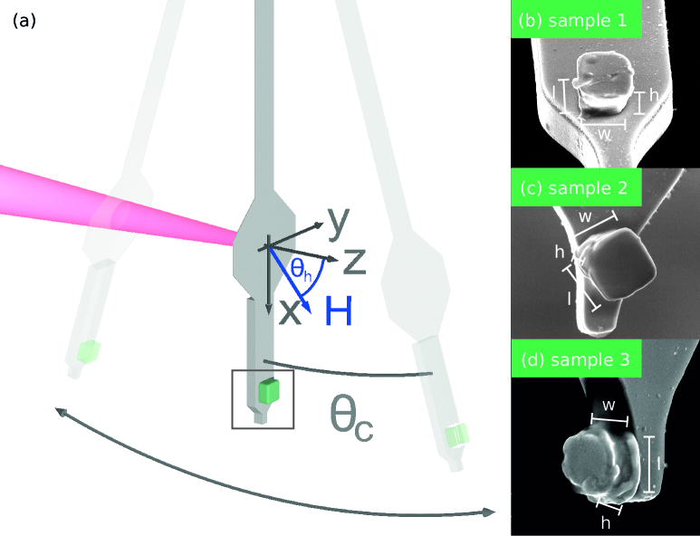
Figure 1: Sketch of the experiment and image of the samples. (a) An infrared laser, focused on the cantilever paddle, allows interferometric readout of the cantilever position. An externally applied, homogeneous magnetic field $\mathbf{H}$ can be rotated around the cantilever rotation axis $\mathbf{\hat{y}}$, spanning an angle $\theta_{h}$ with the $z$-axis. The magnetic specimen under investigation is shown as a green cube. (b)-(d) SEM images of the investigated mesocrystals attached to cantilevers. The length $l$ $\times$ width $w$ $\times$ height $h$ of the samples are determined from the images to be $$1.95\text{\,}\mathrm{\SIUnitSymbolMicro m}$\times$1.87\text{\,}\mathrm{\SIUnitSymbolMicro m}$\times$1.58\text{\,}\mathrm{\SIUnitSymbolMicro m}$$, $$1.7\text{\,}\mathrm{\SIUnitSymbolMicro m}$\times$1.89\text{\,}\mathrm{\SIUnitSymbolMicro m}$\times$1.12\text{\,}\mathrm{\SIUnitSymbolMicro m}$$, and $$1.55\text{\,}\mathrm{\SIUnitSymbolMicro m}$\times$1.54\text{\,}\mathrm{\SIUnitSymbolMicro m}$\times$1.35\text{\,}\mathrm{\SIUnitSymbolMicro m}$$, for samples 1, 2, and 3, respectively. $h$ is defined to be along the [001] direction of the BCT crystal structure.

$$\Delta f=\frac{f_{0}}{2k_{0}l_{e}^{2}}\left(\left.\frac{\partial^{2}\mathcal{F}}{\partial\theta_{c}^{2}}\right|_{\theta_{c}=0}\right),$$ (1)

where $k_{0}$ is the cantilever’s spring constant, $l_{e}$ its effective length, and $\theta_{c}$ its angle of oscillation. Measurements of $\Delta f$ are particularly useful for identifying magnetic phase transitions [32], because it is discontinuous for both first and second order phase transitions [33], just as the magnetic susceptibility $\chi=\partial^{2}\mathcal{F}/\partial H^{2}$. $\Delta f$ can also provide information on the switching, saturation magnetization, coercivity, and the anisotropy of a magnetic system.

The ultrasensitive cantilevers are fabricated from undoped Si and are $90\text{\,}\mathrm{\SIUnitSymbolMicro m}$-long, $3.5\text{\,}\mathrm{\SIUnitSymbolMicro m}$-wide and $0.1\text{\,}\mathrm{\SIUnitSymbolMicro m}$-thick with a mass-loaded end and a $11\text{\,}\mathrm{\SIUnitSymbolMicro m}$-wide paddle for optical detection, as shown in Fig. 1. The resonance frequency $f_{0}$ of the fundamental mechanical mode used for magnetometry is between 5 and $6\text{\,}\mathrm{kHz}$ with $k_{0}$ and $l_{e}$ $314\text{\,}\mathrm{\SIUnitSymbolMicro}\mathrm{N}\mathrm{/}\mathrm{m}$ and $74\text{\,}\mathrm{\SIUnitSymbolMicro m}$, respectively. Mesocrystals are attached to the tips of ultrasensitive Si cantilevers with nonmagnetic epoxy, using an optical microscope equipped with precision micromanipulators. The sample-loaded cantilever is then mounted in a vibration-isolated closed-cycle cryostat. The pressure in the sample chamber is less than $10^{-6}$ mbar and the temperature can be stabilized between 4 and $300\text{\,}\mathrm{K}$. Using an external rotatable superconducting magnet, magnetic fields up to $4.5\text{\,}\mathrm{T}$ can be applied along any direction spanning $225\text{\,}\mathrm{\SIUnitSymbolDegree}$ in the plane of cantilever oscillation ($xy$-plane), as shown in Fig. 1. This direction is specified by $\theta_{h}$, which is the angle between $\mathbf{H}$ and $\mathbf{\hat{z}}$, where $\mathbf{\hat{x}}$ is parallel to the cantilever’s long axis and $\mathbf{\hat{y}}$ coincides with its axis of oscillation. The cantilever’s flexural motion is read out using a optical fiber interferometer employing $100\text{\,}\mathrm{nW}$ of laser light at $1550\text{\,}\mathrm{nm}$ [35]. A piezoelectric actuator mechanically drives the cantilever at $f_{0}$ with a constant oscillation amplitude of a few tens of nanometers using a feedback loop implemented by a field-programmable gate array. This process enables the fast and accurate extraction of $f_{0}$ from the cantilever deflection signal.

III Samples

The mesocrystal samples are composed of nanoparticles, which are synthesized following a modified version of the metal oleate route [36, 14]. These particles consist of $\gamma$-Fe₂O₃ (maghemite) with less than $10\text{\,}\mathrm{\char 37\relax}$ Fe₃O₄ (magnetite) content [26, 37]. The nanoparticles have an edge-length of $10.9\text{\,}\mathrm{nm}$, their atomic structure shows a crystalline inverse spinel structure, and their morphology can be described by a rounded cube model [38]. The micron-sized mesocrystals, i.e. 3D superlattices of the maghemite nanocubes arranged with a high degree of both positional and orientational order, have been carefully grown using an optimized evaporation-driven self-assembly process [14, 12, 38]. Small angle X-ray diffraction performed on an individual mesocrystals reveals a body centered tetragonal (BCT) crystal lattice with an in-plane lattice constant $a=$13.47\text{\,}\mathrm{nm}$$, and an out-of-plane lattice constant $c=$15.08\text{\,}\mathrm{nm}$$ [38], cf. Fig. 2 (c) for a cross-sectional transmission electron microscopy (TEM) image of a thinned mesocrystal layer showing the BCT structure. The self-assembly process for the mesocrystals is both size- and shape-selective [12, 38], i.e. the mesocrystals are composed of particles with a size dispersity which is drastically smaller than that in the initial dispersion [38]. Fig. 2 (a) and (b) show scanning electron microscopy (SEM) images of a typical mesocrystal.

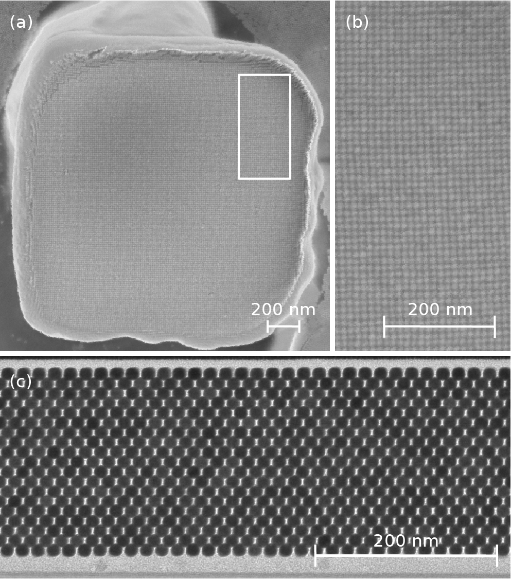
Figure 2: (a) SEM image of a mesocrystal showing the superlattice structure from a top view. (b) Zoom of region shown in (a). (c) Cross-sectional TEM image viewed from the [100] direction of a thinned mesocrystal layer deposited on a Si single crystal, showing the BCT structure. Nanoparticles in the TEM image appear as dark circles.

IV Results and Analysis

We investigate three different mesocrystals, which are each attached in different orientations to the end of a cantilever, as shown Fig. 1. The different orientations allow us to probe the anisotropy in different planes of the superlattice. The crystals have slightly different sizes, which we estimate from SEM images and list in the caption of Fig. 1.

DCM experiments are first carried out at $T=$270\text{\,}\mathrm{K}$$.

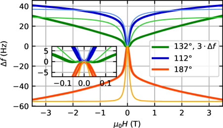
Figure 3: DCM measurements at $270\text{\,}\mathrm{K}$. Dark thick lines show measured $\Delta f(H)$ in sample 1 for orientations $\theta_{h}=$112\text{\,}\mathrm{\SIUnitSymbolDegree}$$, $187\text{\,}\mathrm{\SIUnitSymbolDegree}$ (blue and orange) and $\Delta f(H)$ in sample 3 for $\theta_{h}=$132\text{\,}\mathrm{\SIUnitSymbolDegree}$$ (green). Light thin lines with similar coloring show the corresponding simulations according to a model for a thermally activated Stoner-Wohlfarth particle. The inset shows an enlargement around $H=0$.

In Fig. 3, we plot $\Delta f(H)$ measured in samples 1 and 3, where the external field is swept between $H=\pm$3.5\text{\,}\mathrm{T}$$ for three orientations of $\theta_{h}$. Most DCM curves show a V- or V -shape, depending on the orientation of the applied field. At low field, well below magnetic saturation, some curves present a W-shape, as seen in the inset. In this regime, $\Delta f(H)$ shows a small hysteresis with a coercive field of $\mu_{0}H_{c}\approx$10\text{\,}\mathrm{mT}$$ for all three mesocrystals. At high fields, the curves show an asymptotic behavior and approach either a positive or negative $\Delta f$, depending on the orientation of the external field. The presence of this asymptotic frequency shift implies a magnetic anisotropy in the system [31]. A positive (negative) asymptote signifies alignment with a magnetically easy (hard) direction. We further investigate the mesocrystals’ magnetic anisotropy by measuring the DCM frequency shift of the 3 samples as a function of applied field angle $\theta_{h}$ for $\Delta f(H=$3.5\text{\,}\mathrm{T}$/\mu_{0},\theta_{h})$, at which the samples are near magnetic saturation. The bulk value of the saturation magnetization $M_{s}$ is approximately $3\times 10^{5}$\mathrm{A}\mathrm{/}\mathrm{m}$=$0.38\text{\,}\mathrm{T}$/\mu_{0}$ [6]. Fig. 4 shows polar plots of these measurements, which show evidence of multi-axial anisotropy, most clearly in the case of sample 3.

IV.1 High-field Limit

In order to understand these measurements, we consider the contributions of the possible types of magnetic anisotropy. For a system with uniaxial anisotropy only, set by a uniaxial anisotropy constant $K_{u1}$ (assuming higher order terms are negligible, e.g. $K_{u2}=0$), the frequency shift in the limit of large applied field, i.e. $H\gg|K_{u1}/(\mu_{0}M_{s})|$, is given by [31]

$$\begin{split}\Delta f_{\text{uniaxial}}=&\frac{K_{u1}Vf_{0}}{4k_{0}l_{e}^{2}}\bigg{(}\cos 2\theta_{h}\Big{(}1+3\cos 2\theta_{h}-2\cos 2\phi_{u}\\ &\sin^{2}\theta_{u}\Big{)}+4\cos\phi_{u}\sin 2\theta_{h}\sin 2\theta_{u}\bigg{)},\end{split}$$ (2)

where $V$ is the volume of the magnetic object. $\theta_{u}$, $\phi_{u}$ and $\theta_{h}$ denote the orientation of the anisotropy axis and the external field, respectively. Because the external field is restricted to the $xz$-plane in our setup, no azimuthal angle of the applied field appears in the equation. Similar contributions can be deduced for other types of anisotropy. For cubic anisotropy (again assuming higher order terms are negligible, e.g. $K_{c2}=0$), in the limit of large applied field, i.e. $H\gg|K_{c1}/(\mu_{0}M_{s})|$, we find:

$$\begin{split}\Delta f_{\text{cubic}}=&-\frac{K_{c1}Vf_{0}}{8k_{0}l_{e}^{2}}\cdot\bigg{(}\cos 2\theta_{h}+7\cos 4\theta_{h}\\ &-2\Big{(}1+2\cos 2\theta_{h}\Big{)}\cos 4\phi_{u}\sin^{2}\theta_{h}\bigg{)}.\end{split}$$ (3)

In this case, one of the three anisotropy vectors is assumed to be orthogonal to the cantilever plane ($\mathbf{\hat{u}_{3}}\parallel\mathbf{\hat{z}}$). Therefore, $\mathbf{\hat{u}_{1}}$ and $\mathbf{\hat{u}_{2}}$ lie in the $xy$-plane, and $\phi_{u}$ is the angle between $\mathbf{\hat{u}_{1}}$ and $\mathbf{\hat{x}}$. In light of these relations, we analyze the measured dependence $\Delta f(H=$3.5\text{\,}\mathrm{T}$/\mu_{0},\theta_{h})$ in Fig. 4. To fit the measurements, we find that a sum of a uniaxial, cf. eq. (2), and a cubic, cf. eq. (3), anisotropy is required. A quantitative determination of $K_{u1}$ and $K_{c1}$ is not possible from these particular fits, because $4.5\text{\,}\mathrm{T}$, which is the highest field that we can apply in our apparatus, does not fully satisfy the high-field limit. We can, however, determine the relative weight of the two contributions to the anisotropy.

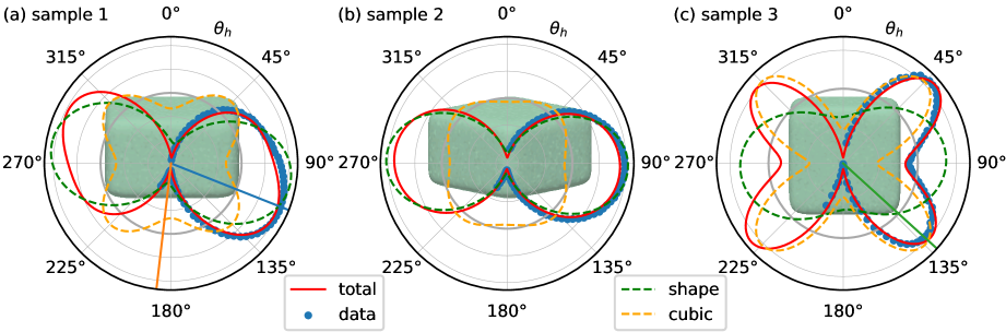
Figure 4: Angular dependence of DCM in the high-field limit. (a)-(c) Polar plots of the high-field frequency shift $\Delta f(H=$3.5\text{\,}\mathrm{T}$/\mu_{0},\theta_{h})$ for sample 1 to 3 (blue dots) and corresponding fits (red, dashed green, and dashed orange lines). Straight, radial lines indicate the direction of the measurements and calculations in Fig. 3, according to the color code. Gray polar lines indicate $\Delta f$ in steps of (a, b) $20\text{\,}\mathrm{Hz}$ and (c) $10\text{\,}\mathrm{Hz}$, with a thick line for $\Delta f=0$. In (a) a sketch of the mesocrystal is shown in the background to illustrate its orientation.

The cubic shape of the nanoparticles within a mesocrystal and the fact that random fluctuations in the shape of individual particles average out over the entire mesocrystal allows us to neglect uniaxial anisotropy due to the shape of individual nanoparticles. Therefore, we assume any observed uniaxial anisotropy to be the result of an effective shape anisotropy of the mesocrystal as a whole. The dipolar interactions between the nanoparticles and, therefore, the shape and lattice spacing of the mesocrystal determine this effective shape anisotropy, in analogy to the shape anisotropy of a continuous magnetic solid [39, 40]. A 1D equivalent of such an effective anisotropy has previously been used to describe chains of iron oxide nanoparticles [13, 41]. Micromagnetic simulations show that this effective magnetic shape anisotropy is dominated by the overall shape of the mesocrystal samples, rather than by the small difference between the in- and out-of-plane lattice spacings of their BCT lattice (cf. Appendix C.2).

A cubic component of the anisotropy may be present in the mesocrystals as a result of the cubic shape of the overall mesocrystal or of the individual maghemite nanoparticles [42], their crystalline anisotropy [43, 44], or their surface anisotropy, as suggested in Refs. 45, 46, 47. The latter is calculated to be relevant only for particles with up to about 100 atoms per dimension, which is exceeded by our nanoparticles. Micromagnetic simulations show that the contribution from the cubic shape of the mesocrystals and the constituent nanoparticles are both at least one order of magnitude too small to account for the anisotropy observed in our DCM measurements (cf. Appendix C.1). On the other hand, the crystalline contribution should appear in our measurements, due to the alignment of the individual nanoparticles with respect to each other.

Indeed, in all three mesocrystal orientations shown in Fig. 4, both the uniaxial and the cubic components of the fitted curves match the expected orientation of the mesocrystal and its constituent crystalline nanoparticles. Furthermore, the magnitude of the uniaxial term is seen to scale with the overall shape of the mesocrystals: e.g. sample 3, the most symmetric mesocrystal (cf. caption of Fig. 2), shows a nearly vanishing uniaxial anisotropy.

IV.2 Full Field Dependence

In order to extract quantitative values for the uniaxial and cubic anisotropies and to understand the full field dependence of the measured $\Delta f(H)$ curves shown in Fig. 3, including the low-field regime, we develop a model of the entire DCM response. Although such models are well-established for ferromagnetic systems, through a simple Stoner-Wohlfarth approach [31] or using micromagnetic simulations [31, 48, 49], no such framework exists for superparamagnetic systems. At $T=$270\text{\,}\mathrm{K}$$ we expect individual maghemite cubes of the given dimensions to be superparamagnetic, despite being embedded in a superlattice structure [13]. The dense arrangement of the nanoparticles within a mesocrystal involves significant inter-particle dipolar interactions. These interactions alter the magnetic behavior of the system, resulting in a shifted blocking temperature, hysteresis, or even a suppression of superparamagnetism. Below the blocking temperature, we expect the system to become ferromagnetic.

We follow Ref. 50 to develop a DCM model for the simplest superparamagnet: an individual, thermally activated Stoner-Wohlfarth particle. To do so, an effective single particle Hamiltonian is constructed, and the corresponding partition function and free energy $\mathcal{F}$ are numerically calculated. Then, thermodynamic quantities are extracted by determining the corresponding derivatives, as shown in Appendix A. In the case of DCM, $\Delta f$ can be found according to eq. (1). In Appendix B, we verify the applicability of this model by recovering the ferromagnetic Stoner-Wohlfarth response, as calculated in Ref. 31, for a thermally activated particle with only magnetic shape anisotropy in the low temperature limit. In this model, paramagnetic behavior sets in as the temperature is increased.

For a mesocrystal of superparamagnetic nanoparticles, we then consider $n$ interacting superparamagnets, where $n$ is the number of nanoparticles in the mesocrystal lattice. Each obeys an effective Hamiltonian, which includes both uniaxial and cubic magnetic anisotropy terms. The uniaxial term reflects the dipolar interactions between particles, i.e. the effective shape anisotropy of the whole mesocrystal, and the cubic term reflects the crystalline anisotropy of each particle. Because we model the inter-particle interaction with an effective single particle term in the Hamiltonian, the model has limited validity, similar to approaches relying on mean-field Hamiltonians [51]. Model parameters for each mesocrystal are summarized in Appendix A. $n$ is estimated from the mesocrystal dimensions, as determined from SEM images and adjusted to match the measurements at high field. To account for the expected presence of a disordered surface spin layer and to adequately fit the data, we model the individual maghemite particles to be slightly smaller, $9$ rather than $10.9\text{\,}\mathrm{nm}$ on a side. $M_{s}$ is taken to be $3\times 10^{5}$\mathrm{A}\mathrm{/}\mathrm{m}$$ [6]. We use the same magnitude of $K_{c1}$ for all mesocrystals, since this term represents the crystalline anisotropy of the individual maghemite nanoparticles, and set it to $-3.0\text{\,}\mathrm{k}\mathrm{J}\mathrm{/}\mathrm{m}^{3}$ to best match the measurements. This value is smaller than the $-4.7\text{\,}\mathrm{k}\mathrm{J}\mathrm{/}\mathrm{m}^{3}$ of bulk $\gamma\text{-Fe}_{2}\text{O}_{3}$, perhaps due to interparticle interactions [52]. Fitting the data also yields $K_{u1}=9.7$, $20.8$, and $2.1\text{\,}\mathrm{k}\mathrm{J}\mathrm{/}\mathrm{m}^{3}$ or $D_{u}=-0.17$, $-0.37$, and $-0.04$ in terms of the effective demagnetization factor for samples 1, 2, and 3, respectively. All of these values should be treated as approximate, given the simpleness of the model and the uncertainty (up to $20\%$) in precisely determining the magnetic volume of the mesocrystal samples.

Calculated $\Delta f(H)$ curves are plotted along with measured $\Delta f(H)$ curves for the same field orientations in Fig. 3. The model adequately captures the overall features of the measurements, including V-, V -, and W-shapes. This agreement is evidence that the particles making up the mesocrystals are indeed in a superparamagnetic state at $T=$270\text{\,}\mathrm{K}$$. Most notably, the V -shape is observed for a hard axis alignment of the external field (yellow curve) and is in strong contrast to the signature of a ferromagnet (cf. Appendix B). The model also explains the occurrence of W-shaped curves: it is a consequence of the opposing sign of the cubic crystalline and the uniaxial shape anisotropy contributions for certain orientations of the external field, e.g. for $\theta_{h}\approx$135\text{\,}\mathrm{\SIUnitSymbolDegree}$$, cf. Fig. 4 (c). A pure cubic system in this orientation leads to a relatively broad V-shape, while a pure uniaxial system leads to a relatively sharp V -shape with a small negative high-field asymptote. The presence of both anisotropies and their resultant competition produces a W-shaped curve.

Despite this agreement, the model predicts high-field $\Delta f(H)$ asymptotes that saturate at lower field than in experiment, presumably as a consequence of the interactions between the particles, which we do not fully consider. Furthermore, in contrast to the experiments, the model does not predict hysteresis as a function of $H$. However, introducing strong interactions (e.g. with a mean field approach) or large anisotropies (increasing the anisotropy constants) to the model leads to ferromagnetic behavior, which includes hysteresis. We thus hypothesize that the observed hysteresis originates from the presence of the inter-particle interactions.

IV.3 Behavior at low temperature

Temperature dependent measurements of the DCM response down to $5\text{\,}\mathrm{K}$ allow us to extract further information about the mesocrystals. Measurements of $\Delta f(T)$ after a mesocrystal is cooled in an applied field, i.e. field cooling (FC), and in zero field, i.e. zero-field cooling (ZFC) show the onset of ferromagnetism below a superparamagnetic blocking temperature $T_{b}^{\text{spm}}\approx$133\text{\,}\mathrm{K}$$, as discussed in Appendix D. Furthermore, measurements of magnetic hysteresis in $\Delta f(H)$ as a function of decreasing temperature show that a more complicated magnetic state emerges at lower temperatures. In particular, measurements show an exchange bias field $H_{\text{eb}}$ emerging below a blocking temperature of $T_{b}^{\text{eb}}\approx$90\text{\,}\mathrm{K}$$. Just below $50\text{\,}\mathrm{K}$ the coercivity $H_{c}$ is seen to increase dramatically, possibly indicating a magnetic transition of unknown origin.

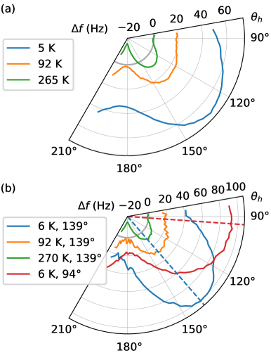
Figure 5: High-field frequency shift $\Delta f(H=$3.5\text{\,}\mathrm{T}$/\mu_{0},\theta_{h})$ for sample 3 depending on the external field direction for various temperatures. The sample undergoes (a) ZFC and (b) FC. The magnetic field for FC is applied at the angle indicated by the color-coded dashed line.

Fig. 5 shows high-field DCM data, similar to that shown in Fig. 4 (a)-(c), measured at different temperatures under both ZFC and FC. The measurements show that under ZFC, shown in Fig. 5 (a), while the shape of $\Delta f(\theta_{h})$ is preserved down to $5\text{\,}\mathrm{K}$, its magnitude increases with decreasing temperature. This behavior indicates an increase of either the anisotropy, the saturation magnetization, or both. Measurements under FC give similar results as those under ZFC regardless of the FC field direction for all but the lowest temperature measurements. Below $90\text{\,}\mathrm{K}$, however, the shape, orientation, and magnitude of the signal change for ZFC and FC. The direction of the maximum in $\Delta f(\theta_{h})$ is observed to follow the direction of the FC field. This reorientation of the magnetic anisotropy by the FC field is observed both when the sample is cooled in an external field applied at $139\text{\,}\mathrm{\SIUnitSymbolDegree}$ and $94\text{\,}\mathrm{\SIUnitSymbolDegree}$, as shown in Fig. 5 (b). Upon heating above $90\text{\,}\mathrm{K}$, the original shape and magnitude of $\Delta f(\theta_{h})$ is restored.

Similar observations have been made in dilute systems of particles, where inter-particle interactions are negligible [53, 9]. As in those and similar studies [54, 55, 56], including small angle neutron scattering measurements [7, 8], we conclude that the individual nanoparticles are likely surrounded by a disordered system of surface spins. Below $T_{b}^{\text{eb}}$, these spins freeze, leading to the observed exchange bias and an additional magnetic anisotropy that can be set and oriented by FC.

Given the agreement of these previous measurements with our data, we find that frozen surface spins are more likely to explain the observed exchange bias and anisotropy than frustration of the core spins in our densely-packed superlattice of nanoparticles. Nevertheless, the configuration of the core spins at low temperatures remains unknown. States such as superferromagnetic and superantiferromagnetic [4] ordering or a superspin glass [57] are potentially present. Further experiments, such as real space imaging or aging experiments are necessary to pin down the mesocrystal’s low-temperature magnetic configuration. The kink in the temperature dependence of $H_{c}$ around $50\text{\,}\mathrm{K}$, which is discussed in Appendix E, may be an indication of a phase transition of such a superspin state.

V Conclusion

In conclusion, our measurements reveal the different contributions to the magnetic anisotropy of a mesocrystal of maghemite nanoparticles, most notably a cubic component, which we attribute to the crystalline anisotropy of the constituent nanoparticles. A model considering interacting superparamagnetic nanoparticles captures most of our findings. The system remains in a superparamagnetic state down to $T_{b}^{\text{spm}}\approx$133\text{\,}\mathrm{K}$$. Below $T_{b}^{\text{eb}}\approx$90\text{\,}\mathrm{K}$$, exchange bias and a frozen spin state are present in the system, consistent with a disordered layer of surface spins on the individual nanoparticles, as observed in earlier works.

We emphasize that the observation of cubic magnetic anisotropy in these nanoparticles is only possible, because of the combination of two techniques: the size-selective self-assembly of nanoparticle mesocrystals with a narrow size distribution and a high degree of orientational order [12, 38], and measurement by DCM, which is sensitive enough to resolve the magnetism of individual mesocrystals. This ability to isolate the magnetic response of a single mesocrystal overcomes the limitations of measuring ensembles, which are composed of mesocrystals of varying size, shape, and orientation. This disorder and the potential for interactions between mesocyrstals complicates the determination of their individual magnetic properties and those of their constituent nanoparticles, especially anisotropy. In the future, similar techniques combining self-assembly and DCM may become a powerful means for assessing the magnetic properties of other nanoparticles, which are too small to investigate individually.

Appendix A Model for DCM response

We follow Ref. 50 to establish a model for the DCM response of an individual, thermally activated Stoner-Wohlfarth particle. We consider a particle with saturation magnetization $M_{s}$, volume $V$, uniaxial anisotropy constant $K_{u1}$, and cubic anisotropy constant $K_{c1}$. The magnetization vector of the macrospin is given by $\mathbf{M}=M_{s}\cdot\mathbf{\hat{m}}$, where $\mathbf{\hat{m}}$ is a unit vector. The unit vector defining the uniaxial anisotropy is given by $\mathbf{\hat{u}}$ and the unit vectors defining the cubic anisotropy are $\mathbf{\hat{u}_{i}}$ with $i=1,2,3$. For simplicity, we do not consider higher order anisotropies. The Hamiltonian of the magnetic system is then given by $\mathcal{H}=\mathcal{H}_{\text{Zeeman}}+\mathcal{H}_{\text{uniaxial}}+\mathcal{H}_{\text{cubic}}$, where,

$$\mathcal{H}_{\text{Zeeman}}=-\mu_{0}\mathbf{M}\cdot\mathbf{H}V,$$ (4)

$$\mathcal{H}_{\text{uniaxial}}=-K_{u1}V\left(\mathbf{\hat{m}}\cdot\mathbf{\hat{u}}\right)^{2},$$ (5)

$$\begin{split}\mathcal{H}_{\text{cubic}}=-VK_{c1}&\Big{(}\left(\mathbf{\hat{m}}\cdot\mathbf{\hat{u}_{1}}\right)^{2}\left(\mathbf{\hat{m}}\cdot\mathbf{\hat{u}_{2}}\right)^{2}\Big{.}\\ &+\left(\mathbf{\hat{m}}\cdot\mathbf{\hat{u}_{2}}\right)^{2}\left(\mathbf{\hat{m}}\cdot\mathbf{\hat{u}_{3}}\right)^{2}\\ &\Big{.}+\left(\mathbf{\hat{m}}\cdot\mathbf{\hat{u}_{3}}\right)^{2}\left(\mathbf{\hat{m}}\cdot\mathbf{\hat{u}_{1}}\right)^{2}\Big{)}.\end{split}$$

By substituting $-\frac{\mu_{0}}{2}D_{u}M_{s}^{2}$ for $K_{u1}$, the uniaxial anisotropy can be expressed as a shape anisotropy, where $D_{u}$ is the effective demagnetization factor [39, 40]. We incorporate oscillations of the cantilever, which correspond to rotations of $\mathbf{\hat{u}}$ and $\mathbf{\hat{u}_{i}}$ about $\mathbf{\hat{y}}$ by an oscillation angle $\theta_{c}$, by applying a rotation matrix $\mathbf{\widetilde{R}}(\theta_{c})$ to all $\mathbf{\hat{u}}$ and $\mathbf{\hat{u}_{i}}$. The partition function of the system is given by:

$$\mathcal{Z}=\frac{1}{2\pi}\int^{\pi}_{0}\mathop{}\!\mathrm{d}\theta_{m}\sin\theta_{m}\int^{2\pi}_{0}\mathop{}\!\mathrm{d}\phi_{m}\exp\left[-\frac{\mathcal{H}\left(\theta_{m},\phi_{m}\right)}{k_{B}T}\right],$$ (6)

where $\theta_{m}$ and $\phi_{m}$ are the polar and azimuthal angles of $\mathbf{\hat{m}}$. This yields the free energy, through $\mathcal{F}=-k_{b}T\ln\mathcal{Z}$. Once all parameter values are set, the integral over $\theta_{m}$ and $\phi_{m}$ can be evaluated numerically. Using the difference quotient to approximate the second derivative, we then calculate the frequency shift of the cantilever,

$$\Delta f=\frac{f_{0}}{2k_{0}l_{e}^{2}}\left(\frac{\partial^{2}\mathcal{F}}{\partial\theta_{c}^{2}}\right)\approx\frac{f_{0}}{2k_{0}l_{e}^{2}}\frac{\mathcal{F}\left(\theta_{c}\right)-2\mathcal{F}\left(0\right)+\mathcal{F}\left(-\theta_{c}\right)}{\theta_{c}^{2}}.$$ (7)

For the model fits shown in Fig. 3, we use a temperature of $T=$270\text{\,}\mathrm{K}$$, a saturation magnetization of $M_{s}=3\times 10^{5}$\mathrm{A}\mathrm{/}\mathrm{m}$$, a cubic anisotropy constant of $K_{c1}=$-3.0\text{\,}\mathrm{k}\mathrm{J}\mathrm{/}\mathrm{m}^{3}$$ and a volume of the individual nanoparticles of $(9$\mathrm{nm}$)^{3}$. The particle number is taken to be $n=1.87\times 10^{6}$, $0.83\times 10^{6}$ and $1.67\times 10^{6}$ and the uniaxial anisotropy constant $K_{u1}=9.7$, $20.8$, and $2.1\text{\,}\mathrm{k}\mathrm{J}\mathrm{/}\mathrm{m}^{3}$ (or $D_{u}=-0.17$, $-0.37$, and $-0.04$) for samples 1,2 and 3, respectively. The cantilever properties are $k_{0}=$314\text{\,}\mathrm{\SIUnitSymbolMicro}\mathrm{N}\mathrm{/}\mathrm{m}$$ and $l_{e}=$74\text{\,}\mathrm{\SIUnitSymbolMicro m}$$, and the angular oscillation amplitude is $\theta_{c}=1.5^{\circ}$.

Appendix B Modeling a superparamagnetic particle

As an example of the DCM model discussed in Appendix A, we calculate $\Delta f$ of a magnetic particle for two different temperatures, one at $T=$5\text{\,}\mathrm{K}$$ leading to a blocked state and the other one at $T=$300\text{\,}\mathrm{K}$$ leading to a superparamagnetic state. The particle has a magnetic shape anisotropy, given by the effective demagnetization factor $D_{u}$. We do each calculation for two different orientations of $\mathbf{\hat{u}}$ and $\mathbf{H}$: $\mathbf{\hat{u}}\bot\mathbf{H}$ and $\mathbf{\hat{u}}\parallel\mathbf{H}$, as shown in Fig. 6. We use the following parameters: $f_{0}=$5\text{\,}\mathrm{kHz}$$, $l_{e}=$100\text{\,}\mathrm{\SIUnitSymbolMicro m}$$, $k_{0}=$100\text{\,}\mathrm{\SIUnitSymbolMicro}\mathrm{N}\mathrm{/}\mathrm{m}$$, $\theta_{c}=$1\text{\,}\mathrm{\SIUnitSymbolDegree}$$, $V=$1000\text{\,}\mathrm{n}\mathrm{m}^{3}$$, $M_{s}=$300\text{\,}\mathrm{k}\mathrm{A}\mathrm{/}\mathrm{m}$$, $D_{u}=-0.1$, $\theta_{h}=\phi_{u}=0$, and $\theta_{u}=$0\text{\,}\mathrm{\SIUnitSymbolDegree}$$, and $90\text{\,}\mathrm{\SIUnitSymbolDegree}$.

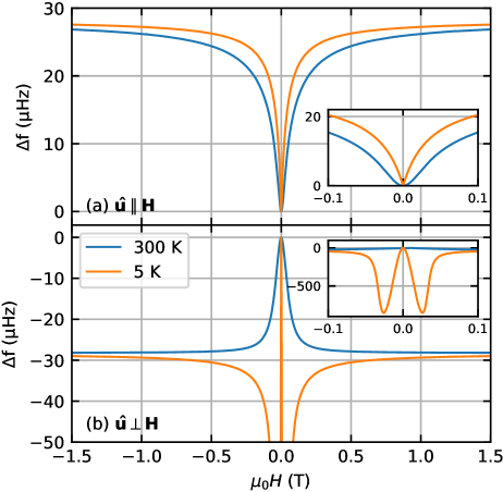
Figure 6: Simulation of DCM for an individual, thermally-activated Stoner-Wohlfarth particle at $T=300$ and $5\text{\,}\mathrm{K}$. Simulated $\Delta f(H)$ with (a) $\mathbf{\hat{u}}\parallel\mathbf{H}$, and (b) $\mathbf{\hat{u}}\bot\mathbf{H}$.

In the $\mathbf{\hat{u}}\parallel\mathbf{H}$ configuration, the difference between the curves at $300\text{\,}\mathrm{K}$ and $5\text{\,}\mathrm{K}$ is small: the curve at $300\text{\,}\mathrm{K}$ is broader and approaches the horizontal asymptote more slowly than the curve at $5\text{\,}\mathrm{K}$. In the $\mathbf{\hat{u}}\bot\mathbf{H}$ configuration, however, the curves behave in a fundamentally different way. The curve at $300\text{\,}\mathrm{K}$ is similar to the case of $\mathbf{\hat{u}}\parallel\mathbf{H}$, but mirrored across $\Delta f=0$. The curve at $5\text{\,}\mathrm{K}$ has a distinct W-shape for low fields, cf. the inset, approaching the horizontal asymptote from negative rather than positive values of $\Delta f$. This curve matches the DCM curves calculated from the ferromagnetic Stoner-Wohlfarth model of Ref. 31. There is a difference at low fields, where $\Delta f$ becomes positive in Ref. 31, but not in the model here. We ascribe this to the different approaches to the problem: here, we have a statistical model, that considers thermal excitation of the magnetization. In Ref. 31, a direct energy minimization leads to the equilibrium magnetization and temperature is not considered. In the $\mathbf{\hat{u}}\perp\mathbf{H}$ case, the distinction between the V - and W-shape of the DCM curve can be used to identify the para- or ferromagnetic state of a magnetic specimen.

To understand the progression of $\mathbf{M}$ with external field, it is instructive to look at the equilibrium probability distribution of magnetic moments, which is given by

$$P_{e}\left(\theta_{m},\phi_{m}\right)=\frac{\exp\left[-\mathcal{H}\left(\theta_{m},\phi_{m}\right)/k_{b}T\right]}{\mathcal{Z}}.$$ (8)

Integrating $P_{e}$ over $\phi_{m}$ and plotting it as a function of $m_{z}=M_{z}/M_{s}=\cos\left(\theta_{m}\right)$ for a few values of the external field, illustrates the difference between the blocked and the superparamagnetic state, cf. Fig. 7. In (a), we plot the probability for $\mathbf{\hat{u}}\parallel\mathbf{H}$ and $H=0$. For the ferromagnet at $5\text{\,}\mathrm{K}$ (green), there are very sharp maxima at $m_{z}=\pm 1$. This means that $\mathbf{M}$ favors alignment with $\mathbf{\hat{u}}$, with parallel and anti-parallel alignment being equally probable. Away from these two peaks, $P_{e}$ is essentially zero, i.e. the magnetization is very unlikely to point in any direction other than along $\mathbf{\hat{u}}$. Turning on a slight external field ($\mu_{0}H=$10\text{\,}\mathrm{mT}$$), the peak at $m_{z}=-1$ vanishes, and only $m_{z}=+1$ is favored (red curve). Although not obvious in the DCM curves, $P_{e}$ shows how this behavior differs from the paramagnetic behavior at $300\text{\,}\mathrm{K}$ (blue and orange curves). Here, $\mathbf{M}\parallel\mathbf{\hat{u}}$ is still favored, but the probability for $\mathbf{M}$ to point in any other direction is not negligible. Turning on a small external field has a much smaller effect on $P_{e}$ at $300\text{\,}\mathrm{K}$ than at $5\text{\,}\mathrm{K}$, which explains why the DCM curve for the paramagnetic case is broader than the ferromagnetic one. Similar effects can be observed for $\mathbf{\hat{u}}\bot\mathbf{H}$, cf. Fig. 7 (b). In general, when an external field is applied, $\mathbf{M}$ rotates from being aligned with $\mathbf{\hat{u}}$ towards the direction of $\mathbf{H}$. For the ferromagnetic case, this is manifested in relatively sharp peaks that shift towards $m_{z}=+1$ with increasing field. For the paramagnetic case, very broad probability distributions are present and the macro spin may fluctuate significantly in a broad range of directions.

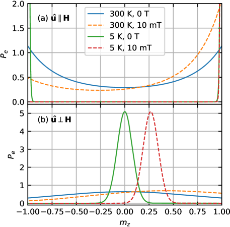
Figure 7: $P_{e}$ for an individual, thermally activated Stoner-Wohlfarth particle with (a) $\mathbf{u}\parallel\mathbf{H}$, and (b) $\mathbf{u}\bot\mathbf{H}$.

Appendix C Micromagnetic simulations

Finite difference simulations are all performed with the Mumax software package [58] using the following parameters, which are determined by the properties of the investigated samples and measurement apparatus: $M_{s}=3\times 10^{5}$ $\mathrm{A}\mathrm{/}\mathrm{m}$, $A_{ex}=10$ $\mathrm{p}\mathrm{J}\mathrm{/}\mathrm{m}\mathrm{{}^{3}}$, $f_{0}=5572.134$ $\mathrm{Hz}$, $k_{0}=314$ $\mathrm{\SIUnitSymbolMicro}\mathrm{N}\mathrm{/}\mathrm{m}$, $l_{e}=73.4$ $\mathrm{\SIUnitSymbolMicro m}$ and $\mu_{0}H=3.5$ $\mathrm{T}$. We minimize the energy of a magnetic state using a steepest descent method [59], and then calculate the frequency shift using eq. (7).

C.1 Cubic shape anisotropy

We analyze the symmetry and magnitude of the shape anisotropy of an individual maghemite nanoparticle by calculating $\Delta f(\theta_{h})$ for a $11\text{\,}\mathrm{nm}$ cube. In the simulations, the cube is discretized in cells with $0.2\text{\,}\mathrm{nm}$ edge length. To estimate the impact of a single cube’s anisotropy on $\Delta f$ of a full mesocrystal, we multiply with the approximate particle number $n\approx 2\times 10^{6}$ in a mesocrystal. The simulation results are shown in Fig. 8 (a) in blue. The symmetry of $\Delta f$ is cubic, as expected, and the magnitude is below $0.5\text{\,}\mathrm{Hz}$ for $\mu_{0}H=3.5$ $\mathrm{T}$. This is far too small to explain the observed magnitude of the cubic component of $\Delta f$ (in the tens of $\mathrm{Hz}$) in experiment. To contrast this result, we add a cubic crystalline anisotropy with $K_{c1}=-$3\text{\,}\mathrm{k}\mathrm{J}\mathrm{/}\mathrm{m}\mathrm{{}^{3}}$$ to the simulation and get a magnitude of $\Delta f$ of around $25\text{\,}\mathrm{Hz}$, which is on the scale of the experimental results. Note that the real particles are rounded cubes as compared to a perfectly shaped cube in the simulation, further reducing the cubic shape anisotropy.

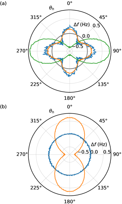
Figure 8: (a) Simulated frequency shift of an individual nanoparticle of $11\text{\,}\mathrm{nm}$ side length multiplied by $2\times 10^{6}$ (blue curve), a symmetric $1\text{\,}\mathrm{\SIUnitSymbolMicro m}$ sized cube (orange curve) and a slightly asymmetric $1\text{\,}\mathrm{\SIUnitSymbolMicro m}$ sized cube (green curve). (b) Simulated frequency shift of a BCT lattice of rounded nanocubes with lattice constants $a=c=$14\text{\,}\mathrm{nm}$$ (blue curve) and $a=$14\text{\,}\mathrm{nm}$$, $c=$16\text{\,}\mathrm{nm}$$ (orange curve).

The same modeling procedure is carried out for a perfectly shaped $1\times 1\times$1\text{\,}\mathrm{\SIUnitSymbolMicro m}\text{\,}{\mathrm{}}^{3}$$ cube, in order to estimate the contribution of the mesocrystal’s overall shape to the cubic component of the observed $\Delta f$. We use a cell size of $10\text{\,}\mathrm{nm}$, which is well below the exchange length of $13.3\text{\,}\mathrm{nm}$ for the used material parameters, and have checked with $5\text{\,}\mathrm{nm}$ cells that the results are robust against a further reduction of the cell size. The simulation results are shown in Fig. 8 (a) in orange. Again, the magnitude of this effect is too small to account for the observed magnitude of the cubic component of $\Delta f$. For comparison, we show the result for a slightly asymmetric cube ($1\times 1\times$0.99\text{\,}\mathrm{\SIUnitSymbolMicro m}\text{\,}{\mathrm{}}^{3}$$) in green. The small asymmetry leads to a strong uniaxial component in $\Delta f$ as compared to the cubic component.

C.2 Anisotropy due to the body centered tetragonal superlattice

The periodicity of a mesocrystal’s superlattice structure affects the effective shape anisotropy (see main text for definition) of the mesocrystal. Depending on the lattice constants, certain directions may have stronger or less strong dipolar interactions. To quantify this influence, we carry out micromagnetic simulations of BCT lattices of rounded cubes with different lattice constants. To avoid uniaxial contributions to the shape anisotropy, resulting from elongation of the mesocrystal in one direction, we choose a cubic simulation volume of $112\text{\,}\mathrm{nm}$ on a side. The cubes themselves have a side length of $10\text{\,}\mathrm{nm}$ and rounded edges by intersecting with a $12\text{\,}\mathrm{nm}$ sphere. We use periodic boundary conditions in all directions with 4 repetitions on each side of the simulation volume, so that edge effects are negligible (half- and quartercubes sitting on the edges and corners of the simulation volume guarantee correct periodicity). In this way, each spatial dimension of the simulated mesocrystal is equally sized with approximately $1\text{\,}\mathrm{\SIUnitSymbolMicro m}$ length. Two sets of lattice constants are chosen, set 1 is $a=c=$14\text{\,}\mathrm{nm}$$ and set 2 $a=$14\text{\,}\mathrm{nm}$$ and $c=$16\text{\,}\mathrm{nm}$$, where $c$ points in $z$-direction in the coordinate system shown in Fig. 1. The calculated $\Delta f(\theta_{h})$ for set 1, which is perfectly symmetric with respect to all three spatial dimensions, is shown as a blue curve in Fig. 8 (b). $\Delta f$ is negligible in all directions compared to the value measured in our experiment. Set 2, for which the cubes have a slightly larger spacing in $z$-direction, shows an easy uniaxial ansiotropy contribution in this direction. However, the magnitude of the effect is around $0.5\text{\,}\mathrm{Hz}$, and hence small compared to the effect of elongations of the mesocrystal in one spatial direction. The lattice constants of set 2 and their difference are very comparable with the values of the experimentally investigated samples ($a=$13.47\text{\,}\mathrm{nm}$$ and $c=$15.08\text{\,}\mathrm{nm}$$), and we thus expect a minor contribution of the superlattice structure on the shape anisotropy of the samples.

Appendix D Measurement of the superparamagnetic blocking temperature

Typically, the blocking temperature $T_{b}^{\text{spm}}$ of a superparamagnetic system is identified by comparing FC to ZFC magnetization measurements [4]. DCM does not give access to the magnetization ($M\propto\partial\mathcal{F}/\partial H$), but rather to the curvature of $\mathcal{F}$ with respect to $\theta_{c}$ ($\Delta f\propto\partial^{2}\mathcal{F}/\partial\theta_{c}^{2}$). $\Delta f$ is hence comparable to the magnetic susceptibility ($\chi\propto d^{2}\mathcal{F}/dH^{2}$). Frequency dependent measurements of $\chi$ allow the identification of $T_{b}^{\text{spm}}$ [4]. Frequency dependent DCM measurements, however, are complicated by the cantilever’s discrete mechanical modes. We can, however, compare FC and ZFC measurements of $\Delta f$. Fig. 9 shows the difference between these frequency shifts, $\Delta f_{\text{ZFC}}-\Delta f_{\text{FC}}$, for sample 3.

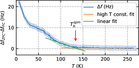
Figure 9: Field cooling data for sample 3. The graph shows the difference between the frequency shift for a zero field cooling and a field cooling measurement in $\mu_{0}H=$125\text{\,}\mathrm{mT}$$.

The mesocrystal is first cooled in zero field; then $\Delta f_{\text{ZFC}}$ is recorded while the sample is heated to room temperature with $125\text{\,}\mathrm{mT}$ of field applied. To measure $\Delta f_{\text{FC}}$, the same procedure is repeated, but with field-cooling in $1\text{\,}\mathrm{T}$. For temperatures above $133\text{\,}\mathrm{K}$ there is no difference between ZFC and FC measurements. Below this temperature, a difference begins to appear, suggesting that the individual nanoparticles stop behaving like superparamagnets and begin behaving like ferromagnets, i.e. they are blocked. Therefore, we conclude that the blocking temperature is $T_{b}^{\text{spm}}\approx$133\text{\,}\mathrm{K}$$ for these mesocrystals.

This temperature compares well with data from ensemble measurements of mesocrystals with similar sizes [12] ($125\text{\,}\mathrm{K}$ for $9.6\text{\,}\mathrm{nm}$ and $155\text{\,}\mathrm{K}$ for $12.6\text{\,}\mathrm{nm}$ particles, while the present ones are $10.9\text{\,}\mathrm{nm}$ sized). Measurements on a dilute ensemble of similar-sized maghemite particles size, but with large silica shells to suppress inter-particle interactions, show $T_{b}^{\text{spm}}\approx$60\text{\,}\mathrm{K}$$[9]. Hence, the interactions between the particles in the mesocrystal appear to increase $T_{b}^{\text{spm}}$ significantly.

Temperature dependent hysteresis data, recorded for sample 2, provide further support for the value of $T_{b}^{\text{spm}}$, cf. Fig. 10.

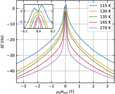
Figure 10: DCM response vs. external field with $\theta_{h}=$180\text{\,}\mathrm{\SIUnitSymbolDegree}$$ for various temperatures around the blocking temperature for sample 2. The curves are offset for better visibility.

With the applied magnetic field aligned along the hard axis, the shape of $\Delta f(H)$ drastically changes at $T_{b}^{\text{spm}}$. Above $T_{b}^{\text{spm}}$, the data match the predictions of our model of interacting superparamagnets. Below $T_{b}^{\text{spm}}$, however, the maximum in $\Delta f$ at zero field transforms into a asymmetric W -shape with two maxima. From the shape of the DCM curves predicted by our model for the para- and ferromagnetic states, we can identify the low-temperature onset of ferromagnetism.

Appendix E Behavior below the superparamagnetic blocking temperature

Hysteresis loops taken at $T=$5\text{\,}\mathrm{K}$$ for sample 3 show that at low temperatures not only superparamagnetism is blocked, but a more complicated magnetic state is present. Depending on the cooling procedure, the measurement proceeds differently, as can be seen in Fig. 11 for measurements with (a) ZFC and (b) FC in $3.5\text{\,}\mathrm{T}$.

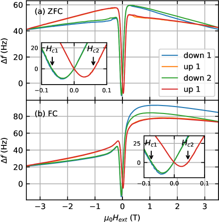
Figure 11: Two consecutive $\Delta f$ hysteresis loops at $5\text{\,}\mathrm{K}$ for (a) ZFC and (b) FC measurements with $\theta_{h}=$184\text{\,}\mathrm{\SIUnitSymbolDegree}$$ for sample 3.

Three main observations can be made from the low temperature measurements: First, the hysteresis loops do not saturate even for the highest applied fields. Second, there is exchange bias [56] present, which can be seen by comparing the positive and negative coercive fields ($\Delta f=0$) in the insets of the figure. Both statements are true irrespective of the cooling procedure. Third, we find a highly asymmetric behavior with respect to the sign of the external field for the FC measurement. The high-field frequency shift differs strongly for positive and negative field values, which is considerably reduced for a second consecutive hysteresis loop. This means that the system can be trained, a typical behavior in a system with an exchange bias. To further understand these findings, we analyze temperature dependent measurements of the coercive field and exchange field.

The blue line in Fig. 12 shows the temperature dependence of the coercive field $H_{c}=\left|H_{c2}-H_{c1}\right|/2$, where $H_{c1}$ ($H_{c2}$) is the negative (positive) coercive field for a ZFC measurement.

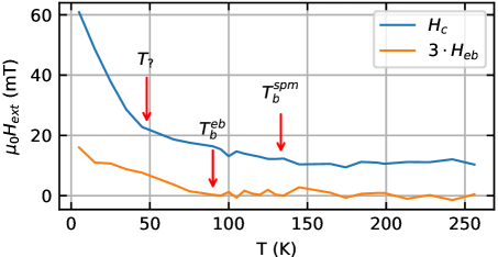
Figure 12: $H_{c}$ and $H_{\text{eb}}$ vs $T$ for zero field cooling in easy anisotropy orientation for sample 2 with $\theta_{h}=$180\text{\,}\mathrm{\SIUnitSymbolDegree}$$.

The coercivity $H_{c}\approx$10\text{\,}\mathrm{mT}$$ is constant above $T_{b}^{\text{spm}}$, as we may expect for a superparamagnetic system with strong interactions. Below $T_{b}^{\text{spm}}$, $H_{c}$ starts to increase, suggesting that the net magnetic moments of an increasing number of nanoparticles switch collectively with decreasing temperature. Just below $50\text{\,}\mathrm{K}$ the curve steepens significantly. This may indicate a magnetic transition of unknown origin.

$H_{c1}$ and $H_{c2}$ show the same magnitude above $90\text{\,}\mathrm{K}$. Below $90\text{\,}\mathrm{K}$, $H_{c1}$ becomes larger than $H_{c2}$ in magnitude. This effect can be quantified by the exchange bias field $H_{\text{eb}}=\left|H_{c2}+H_{c1}\right|/2$ and is shown as orange curve in Fig. 12. From this data, we infer a blocking temperature of the exchange bias effect of $T_{b}^{\text{eb}}\approx$90\text{\,}\mathrm{K}$$. Below $T_{b}^{\text{eb}}$, $H_{\text{eb}}$ increases moderately with decreasing temperature. Doing the same experiment after a FC procedure leads to a significantly enhanced $H_{eb}$.