A Distance-Deviation Consistency and Model-Independent Method to Test the Cosmic Distance-Duality Relation

Abstract

A distance-deviation consistency and model-independent method to test the cosmic distance duality relation (CDDR) is provided. The method is worth attention on two aspects: firstly, a distance-deviation consistency method is used to pair subsamples: instead of pairing subsamples with redshift deviation smaller than a value, say $\left|\Delta z\right|<0.005$. The redshift deviation between subsamples decreases with the redshift to ensure the distance deviation stays the same. The method selects more subsamples at high redshift, up to $z=2.16$, and provides 120 subsample pairs. Secondly, the model-independent method involves the latest data set of $1048$ type Ia supernovae (SNe Ia) and $205$ strong gravitational lensing systems (SGLS), which are used to obtain the luminosity distances $D_{L}$ and the ratio of angular diameter distance $D_{A}$ respectively. With the model-independent method, parameters of the CDDR, the SNe Ia light-curve, and the SGLS are fitted simultaneously. The result shows that $\eta=0.047^{+0.190}_{-0.151}$ and CDDR is validated at 1$\sigma$ confidence level for the form $\frac{{{D_{L}}}}{{{D_{A}}}}{(1+z)^{-2}}=1+\eta z$.

1 Introduction

The cosmic distance duality relation (CDDR), also called Etherington’s reciprocity relation (Etherington, 1933), plays an important role in modern cosmology, especially in galaxy observations (Cunha, Marassi & Shevchuk, 2007; Mantz et al., 2010), cosmic microwave background (CMB) radiation observations (Komatsu et al., 2011), and the gravitational lensing (Ellis, 2007). The CDDR reads

$$\frac{{{D_{L}}}}{{{D_{A}}}}{(1+z)^{-2}}=1,$$ (1)

where $D_{L}$ is the luminosity distance, $D_{A}$ is the angular diameter distance, and $z$ is the redshift. The CDDR is valid for all cosmological models based on Riemannian geometry. The basis of this relation is that the number of photons is conservative and photons travel along the null geodesic in a Riemannian space-time (Ellis, 2007).

The validity of the CDDR is explored widely for the past decades, because any deviation of CDDR may trigger new physics. Uzan et al. (2004) investigates the possible deviation from the CDDR by analysing the measurements of SZE and X-ray emission data of galaxy clusters and reports that the parameter $\eta=0.89^{+0.04}_{-0.03}$ and is at 1$\sigma$ confidence level. Holanda, Lima & Ribeiro (2011) takes more parametrized forms of $\eta$ and found no departure from the CDDR. Nair et al. (2011); Basset & Kunz (2004); Holanda et al. (2010); Holanda, Lima & Ribeiro (2011); Cao & Liang (2011); Meng et al. (2012)used $D_{L}$ directly from type Ia supernovae (SNe Ia) to test the CDDR. Hu, & Wang (2018) and Melia (2018) used the $D_{L}$ form SNe Ia with the $R_{h}=ct$ cosmology model to test the CDDR and compared the model with the $\Lambda$CDM model. Basset & Kunz (2004) found a 2$\sigma$ violation of the CDDR using the luminosity distances $D_{L}$ from SNe Ia and the angular diameter distance $D_{A}$ from FRIIb radio galaxies. Räsänen et al. (2016) used CMB anisotropy to test the CDDR. The CDDR is also important in studying cosmic opacity (Lv & Xia, 2016; Hu et al., 2017).

To test the CDDR, many $D_{L}$ and $D_{A}$ pairs at the same redshift $z$ need to be provided simultaneously. In principle, the two distances should neither be correlated nor based on any cosmology models. That is, a model-independent method and a quality and quantity collection of sample pairs are important. Conventionally, in determining $D_{L}$, the method of Standard Candles (e.g. SNe Ia, GRB (Wang & Dai, 2006; Wang et al., 2007; Wang & Dai, 2008; Wang et al., 2009; Wang & Dai, 2006; Wang et al., 2015; Tu & Wang, 2018; Wang & Wang, 2019)) plays a prominent part. However, the method of Standard Candles is model-dependent, i.e., a special cosmology model is used in calibrating the light-curve parameters. For example, Suzuki et al. (2012) used the cold dark matter (CDM), wCDM, and owCDM models to fit the parameters of Union2.1 SNe Ia and to constrain the cosmology parameters. In determining $D_{A}$, the method of using the Sunyaev–Zel’dovich effect (SZE) and X-ray observations (Cavaliere & Fusco-Fermiano, 1978; Sunyaev & Zel’dovich, 1972; Bonamente et al., 2006) is important in finding $D_{A}$ from galaxy clusters. $D_{A}$ can also be obtained from ultra-compact radio sources (Li & Lin, 2018) and baryon acoustic oscillations (BAOs) (Wu et al., 2015).

There are model-independent methods. Liao et al. (2016) introduced a new method to test the CDDR based on strong gravitational lensing systems and SNe Ia. In their work, they constrain $\eta$, the parameter of the SNe Ia light-curve, and the parameter of the SGLS simultaneously. Räsänen et al. (2016) uses the temperature-redshift relation of CMB to test the CDDR, in their work, a flat FRW universe is assumed. Ruan et al. (2018) use a similar model-independent method with the SGLS, the SNe Ia, and the HII galaxy Hubble diagram to test the CDDR. To avoid the effect of the cosmic opacity, Liao (2019) uses the $D_{L}$ from the gravitational wave signals and the ratio of $D_{A}$ from the SGLS (for details see below) with a model-independent method, which is proposed in (Liao et al., 2016). These model independent methods show that the CDDR is valid in the given redshift range, say, $z<1.0$.

In this paper, we provide a distance-deviation consistency and model-independent method to test the CDDR. The distance-deviation consistency method pairs subsamples with redshift deviation decrease with the redshift to ensure the distance deviation stays the same. It is because the distance grows nonlinearly with the redshift, the larger the redshift is, the smaller the redshift deviation is between two sources with the same distance deviation. The latest data set of SNe Ia with $1048$ samples and strong gravitational lensing system (SGLS) with $205$ samples are involved and the distance-deviation consistency method enables us to take full advantage of the data: the method selects more subsamples at high redshift, up to $z=2.16$, and provide 121 subsample pairs. With the model-independent method, parameters of the CDDR, the SNe Ia light-curve, and the SGLS are fitted simultaneously.

This paper is organized as follows. In Sec.2, we introduce the latest data set of the SNe Ia with $1048$ samples and the SGLS with $205$ samples. In Sec.3, we explain a distance-deviation consistency method to pair subsamples and describe the method of statistical analysis. The numerical results are shown. Conclusions and discussions are given in Sec.4.

2 Data

In this section, we describe two sets of data suitable for testing the CDDR, one based on the redshift and the light-curve of the SNe Ia, from which we can obtain $D_{L}(z)$, the other base on the observational velocity dispersion of the lens galaxy, redshifts of the strong gravitational lensing system (SGLS), from which we can obtain the ratio of $D_{A}(z)$.

2.1 The Pantheon SNe Ia Sample

In this section, we introduce the contents of the Pantheon sample (Scolnic et al., 2018). The Pantheon sample consisting of a total of 1048 SNe Ia in the range of $0.01<z<2.3$ is constructed by a subset include 279 SNe Ia ($0.03<z<0.68$) from the Pan-STARRS1 (PS1) Medium Deep Survey, the Sloan Digital Sky Survey (SDSS), the SNLS, the various low-z, and Hubble Space Telescope (HST) samples.

On one hand, the luminosity distances $D_{L}(z)$ can be determined accurately by multiple light-curve fitters (e.g., (Jha et al., 2007; Guy et al., 2010; Burns et al., 2011; Mandel et al., 2011)). From the phenomenological point of view, the distance modulus, $\mu$, of an SNe Ia can be extracted from its light curve. In a modified version of the Tripp formula (Tripp et al., 1998), the SALT2 light-curve fit parameters are transformed into distances:

$$\mu=m_{B}-M+\alpha x_{1}-\beta c+\Delta_{M}+\Delta_{B},$$ (2)

where $m_{B}$ is the apparent magnitude, $M$ is the absolute B-band magnitude of a fiducial SNe Ia with $x_{1}=0$ and $c=0$, $\Delta_{M}$ and $\Delta_{B}$ are distance corrections based on the mass of the host galaxy of the SNe Ia and predicted biases from simulations respectively. $\alpha$ and $\beta$ are light-curve parameters of relations between the luminosity and the stretch and between the luminosity and the color respectively. Moreover, $\Delta_{M}$ in the equation (2) can be written in the form Scolnic et al. (2018)

$$\Delta_{M}=\gamma[1+e^{(-(m-m_{step})/\tau)}]^{-1},$$ (3)

where $\gamma$, $m_{step}$, and $\tau$ are coefficients to be determined (Scolnic et al., 2018). On the other hand, one assumes that the SNe Ia with identical color, shape, and galactic environment have on average the same intrinsic luminosity for all redshifts (Betoule et al., 2014). According to the definition of the distance modulus, it can be written as

$$\mu=5\log(\frac{D_{L}}{\rm Mpc})+25.$$ (4)

By using equations (2) and (4), we can obtain the luminosity distances $D_{L}(z)$ for the Pantheon SNe Ia Sample.

2.2 The strong gravitational lensing system Sample

For the new SGLS sample, we used from Amante et al. (2019), which contains 205 SGLS. This sample constituted from some survey projects, (e.g. the SLACS, the CASTLES survey, the BELLS, the LSD …). In an SGLS, the light is bent by massive bodies (e.g., galaxy, galaxy cluster) which is predicted by the general theory of relativity. The SGLS is a powerful astrophysical tool to explore the universe and galaxy and has been rapidly developed in recent years, especially like dark energy (Biesiada, 2006; Biesiada et al., 2010; Cao et al., 2012, 2015; Jullo et al., 2010; Magaña et al., 2015, 2018), the CDDR (Liao et al., 2016; Liao, 2019), the cosmic acceleration (Tu et al, 2019), calibrating the standard candles (Wen et al., 2019), and cosmological models’ comparison(Melia et al., 2015; Leaf & Melia, 2018; Tu et al, 2019). In an SGLS, a single galaxy acting as the lens, the Einstein radius depends on three parameters: depends on the angular distance to the source and between the lens and the source, and the mass distribution within the lensing galaxy. A singular isothermal sphere (SIS) model (Ratnatunga et al, 1999) is used to describe the lens galaxy’s mass distribution. The ratio of the angular diameter distances between lens and source and between observer and source can be obtained from a special physical model (e.g. SIS model). Because these distances depend on the cosmological metric, the ratio can be used to constrain cosmological parameters.

In an SIS model of the SGLS, the distance ratio $R^{A}(z_{l},z_{s})$   ($D^{A}_{l}s/D^{A}_{s}$) is related to observables in the following way (Biesiada et al., 2010),

$$R^{A}(z_{l},z_{s})=\frac{c^{2}\theta_{E}}{4\pi\sigma^{2}_{SIS}},$$ (5)

where $c$ is the speed of light, $\theta_{E}$ is the Einstein radius, and $\sigma_{SIS}$ is the velocity dispersion of the stellar in the periphery of the lens galaxy due to the lens mass distribution in the SIS model. In general, $\sigma_{SIS}$ not equals to the observed stellar velocity dispersion $\sigma_{0}$ (White & Davis, 1996). To express the difference, researchers use a phenomenological free parameter $f_{e}$ defined by the relation $\sigma_{SIS}=f_{e}\sigma_{0}$ (Kochanek, 1992; Ofek et al, 2003; Cao et al., 2012), where $(0.8)^{1/2}<f_{e}<(1.2)^{1/2}$. In this case, the systematic error is caused by $\sigma_{0}$ as $\sigma_{SIS}$, the deviation of the SIS model, the effects of secondary lenses (nearby galaxies), the line of sight contamination (Ofek et al, 2003), etc. The uncertainty of equation (5) can be written by (Liao et al., 2016)

$$\sigma_{R^{A}}(z_{l},z_{s})=R^{A}(z_{l},z_{s})\sqrt{(4\delta_{\sigma_{sis}})^{2}+(\delta_{\theta_{E}})^{2}}.$$ (6)

In equation(6), $\delta_{\sigma_{sis}}$ and $\delta_{\theta_{E}}$ are the fractional uncertainty of the $\sigma_{sis}$ and $\theta_{E}$, respectively. To test the CDDR, the left term of equation (ref5), $R^{A}(z_{l},z_{s})$, should be expressed as the ratio of luminosity distance, $D^{A}_{ls}/D^{A}_{s}$. We transform $R^{A}(z_{l},z_{s})$ into the ratio of Comoving distance($D_{C}$) or dimensionless distance $H_{0}D_{C}/c$. In a flat space, the dimensionless distance satisfies

$$d(z_{l},z_{s})=d(z_{s})-d(z_{l}).$$ (7)

By using the equation,

$$D_{A}(z)=\frac{D_{C}(z)}{1+z}=\frac{H_{0}d(z)}{c(1+z)},$$ (8)

$R^{A}(z_{l},z_{s})$ can be written as

$$R^{A}(z_{l},z_{s})=1-\frac{(1+z_{l})D_{A}(z_{l})}{(1+z_{s})D_{A}(z_{s})}.$$ (9)

In a non-flat space, the expression of $R^{A}(z_{l},z_{s})$ is more complicated, one can refer to Räsänen et al. (2015). Fortunately, most cosmological tests today support a flat cosmic (Planck Collaboration et al., 2016), in this work, we test the CDD relation in the case where we assume that space-time is flat.

To test the CDDR, equation (1) is rewritten by the parametrization of the deviation:

$$\frac{{{D_{L}}}}{{{D_{A}}}}{(1+z)^{-2}}=1+\eta z.$$ (10)

Combining equations (9) and (10), $R^{A}(z_{l},z_{s})$ can be written as

$$R^{A}_{0}(z_{l},z_{s})=1-\frac{(1+\eta z_{s})(1+z_{s})d_{L}(z_{l})}{(1+\eta z_{l})(1+z_{l})d_{L}(z_{s})}.$$ (11)

By using equation (4), the part $\frac{d_{L}(z_{l})}{d_{L}(z_{s})}$ of equation (11) can be rewritten as

$$\begin{split}\lg[\frac{d_{L}(z_{l})}{d_{L}(z_{s})}]=&0.2\{m_{B}(z_{l})-m_{B}(z_{s})+\alpha[x(z_{l})-x(z_{s})]-\\ &\beta[c(z_{l})-c(z_{s})]+\Delta_{M}(z_{l})-\Delta_{M}(z_{s})\},\end{split}$$ (12)

where, the absolute magnitude of SNe Ia subsample is offset, $z_{l}$ is the redshift of the lens, and $z_{s}$ is the redshift of the sources.

3 Method and results

In this section, we introduce a distance-deviation consistency method of data selection and show the result.

3.1 Method of data selection: a distance-deviation consistency method

To test the CDDR, $D_{L}$ and $D_{A}$ at the same redshift $z$ need to be provided simultaneously. However, redshifts of subsamples from the SGLS and the SNe Ia are different. To take full advantage of the data, one needs to pair the subsamples efficiently. In this section, we provide a distance-deviation consistency method to pair subsamples, which outperforms the conventional method.

The redshift-difference of subsample-pairs in this work is not fixed, and it decreases with the redshifts to ensure the distance deviation of the sources stays the same. The relation between $\Delta z$ and coordinate distance with a cosmology model reads

$$\Delta{d_{c}^{model}(z)}=d_{c}^{model}(z+\Delta z^{model})-d_{c}^{model}(z),$$ (13)

where $R_{h}=ct$ and flat $\Lambda$CDM model with $\Omega_{m}=0.31$(Planck Collaboration et al., 2016) are used. By setting $\Delta d_{c}/d_{c}$ equals 5% and combining equation(13), $\Delta{z}(z)$ can be calculated:

$$\Delta{z}(z)=min\{\Delta{z}^{\Lambda CDM}(z),\Delta{z}^{R_{h}=ct}(z)\},$$ (14)

where the distance formulas of the two cosmology model, $\Lambda$CDM and $R_{h}=ct$ are used. The $R_{h}=ct$ cosmological model was proposed in Melia (2007). In the $R_{h}=ct$ universe, the luminosity distance $D_{L}$ can be written by:

$$D_{L}^{R_{h}=ct}(z)=\frac{c}{H_{0}}(1+z)\ln(1+z)$$ (15)

This model is a Friedmann–Robertson–Walker (FRW) cosmological model, which is obeying the cosmological principle and Weyl’s postulate(Melia, 2007; Melia & Shevchuk, 2012). In $R_{h}=ct$ universe that space expands at a constant rate, rather than an accelerating rate. Theoretically, there are some controversies with this model, which focus on the zero active mass condition $\rho$$+3p=0$(for more details see Melia (2016); Kim, Lasenbyet & Hobson (2016); Melia (2017)). In terms of the fitting of observational data, the model performs relatively well. The originator of this model himself and his collaborators have done extensive work comparing it with the standard model using many different types of observations, and they have found that the $R_{h}=ct$ model is better than the Standard Model(e.g.Melia (2013); Melia&Manoj (2018); Fatuzzo&Melia (2017b); Melia (2014); Wei et al. (2015); Melia (2019)). Additional work by others also illustrates this point(Yu & Wang, 2014; Yuan & Wang, 2015). There is also a lot of work against this model(e.g. Tutusaus et al. (2016); Shafer (2015)) Thus, despite the theoretical controversy, this model has gained some support for the data, and we can use this model jointly with the standard model to select the data.

For a given SGLS subsample, the redshift-dimensionless distance relation, equation(14), is used to acquire a suitable redshift deviation interval. Then, the subsamples of the SNe Ia with redshifts within the interval are selected as the candidate. Finally, the subsample with the smallest redshift-deviation is selected.

Our method outperforms the conventional method in two aspects: (1) information of subsamples at high-redshifts is conserved. To pair subsamples with a slight difference of redshift is a simple and commonly used method. For example, $\Delta z=0.005$ (Holanda et al., 2010, 2012; Holanda, Busti, & Alcaniz, 2016; Li et al, 2011; Nair et al., 2011), $\Delta z=0.006$ (Goncalves, Holanda& Alcaniz, 2012), and $\Delta z=0.003$ (Liao, 2019). Gaussian Process (GP) reconstruction is also a usable method (Zhang, 2014; Ruan et al., 2018). The linear interpolation method is also taken by some researchers (Liang et al., 2013; Hu, & Wang, 2018). These methods reduce the systematic error to an extent but do not consider the distance-deviation consistency. The relation between the distance and the redshift is non-linear: the same redshift deviation at the higher redshift has a smaller distance deviation. For example, some researchers set the $\Delta z=0.005$, the uncertainty of dimensionless distance is 5% at $z\sim 0.1$, the minimum redshift of the subsample we select, but small than 1% at $z\sim 1$ for selecting data with a general cosmology model, so the selecting uncertainty is not the consistency of distance-deviation. The selecting uncertainty of their methods are all ignoring, and if they were taking them into account in their fitting, they had to introduce a cosmological model so that their methods were no longer model-independent. In our approach, although two cosmological models are introduced, they are used to jointly pick the data, breaking the dependence on a single cosmological model when picking the data, and are not introduced into the $\chi^{2}$ function, in other words, the final parameter fit results are independent of the cosmological model. Cao et al. (2017)used a similar method for selecting the data with a $\Lambda$CDM model to fitting the parameters of the ultra-compact radio quasars. At high redshift, in general, subsamples are sparse and matching pairs of subsamples is difficult if a fixed $\Delta z$ is used. The distance deviation consistency method selects more subsamples at high-redshifts.

(2) More subsample pairs are selected. For example, in the work of Liao et al. (2016), they gain only 60 pairs of samples to testing the CDDR. According to figure(1), at z=0.11, the most previously used $\Delta z=0.005$ and the curve of $\Delta d/d$ in this method are intersecting. So, the $\Delta d/d=5\%$ is the maximum allowable uncertainty of dimensionless distance. In other words, if the error of selecting exceeds 5%, the statistical error of our results must be higher than that of previous work. If the error is significantly lower than 5%, the number of data pairs we choose will not be significantly improved. With the method of fixed $\Delta d/d=5\%$, the number of the pairs can reach 68. The data utilization increases by 13.3%. In this work, we have obtained 120 pairs of samples that redshift from 0.11 to 2.16.

A comparison between our method with a fixed $\Delta d/d$ and the conventional method with a fixed $\Delta z$ are shown in figures (1) and (2). In figure (1), the deviation, $\Delta d/d$, falls rapidly with the increase of redshift with $\Delta z$ fixed. The main advantage of a fixed $\Delta d/d$ is shown in figure (2). To conclude, on the one hand, our method maintains more information about subsamples at high-redshifts. On the other hand, our method selects more subsample-pairs thus reduces the systematic error.

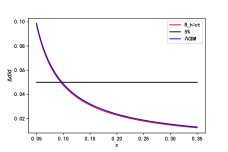
Figure 1: The relation between the $\Delta d/d$ and $z$,the red line and the blue line indicate the relationship between the relative error of $d$ and the redshift in $R_{h}=ct$ model and $\Lambda CDM$ model, respectively. The black line indicates the scheme we used.

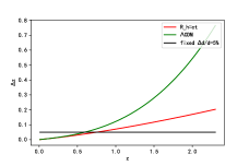
Figure 2: The relation between the $\Delta_{z}$ and $z$

3.2 Method of statistical analysis

To determine the parameters, we minimize $\chi^{2}$ function. By using equations (5) and (11), $\chi^{2}$ function can be written as

$$\chi^{2}=\sum^{120}_{1}(\frac{(R^{A}(z_{l},z_{s})-R^{A}_{0}(z_{l},z_{s}))^{2}}{\sigma^{2}_{R^{A}(z_{l},z_{s})}+\sigma^{2}_{R^{A}_{0}(z_{l},z_{s})}+\sigma^{2}_{sel}}),$$ (16)

where $\sigma_{R^{A}(z_{l},z_{s})}$ is the uncertainty of the SGLS with SIS model, $\sigma_{R^{A}_{0}(z_{l},z_{s})}$ is the error caused by the uncertainty of the distance modulus of SNe Ia, which is related to the uncertainty of observed data (e.g. $m_{B}$), and $\sigma_{sel}$ is the uncertainty of data selection, which is related to artificial selection. By using equation(11), the uncertainty of data selection can be written as

$$\sigma_{sel}=\frac{(1+\eta z_{s})(1+z_{s})d_{L}(z_{l})}{(1+\eta z_{l})(1+z_{l})d_{L}(z_{s})}*\sqrt{(\frac{\Delta d_{l}}{d_{l}})^{2}+(\frac{\Delta d_{s}}{d_{s}})^{2}},$$ (17)

where $\frac{\Delta d_{l}}{d_{l}}=\frac{\Delta d_{s}}{d_{s}}=\frac{\Delta d}{d}=5\%$.

We use the Markov chainMonte Carlo (MCMC) method to constrain the parameters in equation(17). EMCEE (Foreman-Mackey et al., 2013) python package is used. In order to execute the MCMC process, we need to provide the prior values first. In Scolnic et al. (2018), the best value and the 1$\sigma$ confidence level of the parameters are shown. But in our work, we take an SIS model of SGLS to calibrating these parameters, which will different. So, we take the prior interval that completely covering the value range of the value from Scolnic et al. (2018). The prior probability for parameters $P(\alpha,\beta,f_{e},\eta,\gamma,m_{step},\tau)$ is the product of prior probability of each parameter. The prior probability is assumed to be uniform distributions: $P(\alpha)=U[-0.2,0.2]$, $P(\beta)=U[2,6]$, $P(f_{e})=U[0.5,1.5]$, $P(\eta)=U[-0.5,1.5]$, $P(\gamma)=U[0,0.3]$, $P(M_{step})=U[5,15]$, $P(\tau)=U[0.001,1]$. In Pantheon samples, the errors include both statistic and systematic deviation. The systematic error relatives to all data point and appears as a huge covariance matrix. In this work, part of SNe Ia are selected, only the statistic error is considered.

3.3 Results

The result is shown in figure (3) and table (1). Triangle contours are plotted by using the open-source python package “Getdist”. One can see from figure (3) that the best-fitted center value is $\eta=0.047^{+0.190}_{-0.151}$, which is at 1$\sigma$ confidence level. The result indicates that the CDDR is in agreement with the observations and there are no signs of violation in light of SN Ia and SL data.

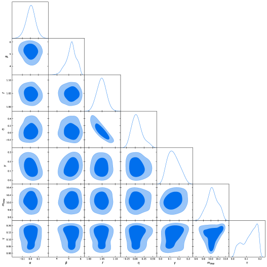
Figure 3: The 2D regionsand 1D marginalized distributions with 1$\sigma$ and 2$\sigma$ contours for the parameters $\alpha$, $\beta$, $f_{e}$, $\gamma$, $m_{step}$,$\tau$ and $\eta$ using Pantheon sample and SGLS sample.

Table 1: Constraints on the coefficients of light-curve parameters and $\eta$ at the 1$\sigma$ confidence levels.

parameters	value
$\alpha$	$0.001^{+0.061}_{-0.061}$
$\beta$	$5.283^{+0.417}_{-0.464}$
$f_{e}$	$1.046^{+0.020}_{-0.019}$
$\eta$	$0.047^{+0.190}_{-0.151}$
$\gamma$	$0.141^{+0.080}_{-0.070}$
$m_{step}$	$10.055^{+0.177}_{-0.148}$
$\tau$	$0.134^{+0.048}_{-0.073}$
$\chi^{2}$	117.430
$\chi^{2}/{d.o.f}$	117.430/113

4 DISCUSSIONS AND CONCLUSIONS

The validation of the CDDR is a crucial topic in cosmology. Any violation of the CDDR may generate a new theory of physics. In recent years, to compare the $D_{L}$ derived from SNe la and the $D_{A}$ measured using galaxy clusters is the common method to test the CDDR. To use this method, a specific cosmology model with some parameters (e.g. the matter density parameter $\Omega_{m}$, the cosmic equation of state, and the Hubble constant) must be assumed. Such results are hardly convincing.

In testing the CDDR, using a model-independent method is necessary. Moreover, to obtain a data sample contains a large number of $D_{L}$ and $D_{A}$ pairs are also important. However, the number of useful subsample pairs is limited by the observed data, and pair subsamples with redshift-deviation smaller than a constant will lose the subsamples at high redshift which leads to systematic errors.

In this paper, we provide a distance-deviation consistency and a model-independent method to test the CDDR. By applying the distance-deviation consistency method on the latest data set of SNe Ia with $1048$ samples and strong gravitational lensing system (SGLS) with $205$ samples, we obtain the collection of subsample pairs not only contains more subsamples but also maintains the information of subsamples at high redshift, up to $z=2.16$. By applying a model-independent method: the SGLS model is used to replace the cosmology model in SNe Ia light-curve fitting, the result shows that $\eta=0.047^{+0.190}_{-0.151}$ and CDDR is validated at 1$\sigma$ confidence level for the form $\frac{{{D_{L}}}}{{{D_{A}}}}{(1+z)^{-2}}=1+\eta z$.

References

- Amante et al. (2019) Amante, M. H., et al. 2019, arXiv:1906.04107
- Basset & Kunz (2004) Basset, B. A., Kunz, M., 2004, PRD, 69, 101305
- Betoule et al. (2014) Betoule, M., et al. 2014, A&A, 568, A22
- Biesiada (2006) Biesiada, M., 2006, PRD, 73, 023006
- Biesiada et al. (2010) Biesiada, M., et al. 2010, MNRAS, 406, 1055
- Bonamente et al. (2006) Bonamente, M., et al. 2006, ApJ, 647, 25
- Burns et al. (2011) Burns, C. R., Stritzinger, M., Phillips, M. M., et al. 2011, AJ, 141, 19
- Cao et al. (2012) Cao, S., et al., 2012, JCAP, 03, 016
- Cao et al. (2015) Cao, S., Biesiada, M., Gavazzi, R., Piorkowska, A., Zhu, Z. U., 2015, ApJ, 806, 185
- Cao et al. (2017) Cao, S., et al. 2017, JCAP, 02, 012
- Cao & Liang (2011) Cao, S., Liang, N., 2011, RAA, 11, 10
- Cavaliere & Fusco-Fermiano (1978) Cavaliere, A., Fusco-Fermiano, R., 1978, A&A., 667, 70
- Cunha, Marassi & Shevchuk (2007) Cunha, J. V., Marassi, L., Lima, J. A. S., 2007, MNRAS, 379, L1
- Ellis (2007) Ellis, G. F. R., 2007, Gen. Relativ. Gravit, 39, 1047
- Etherington (1933) Etherington, I. M. H., 1933, Philos. Mag, 15, 761
- Fatuzzo&Melia (2017b) Fatuzzo, M., &Melia F. 2017, ApJ, 846, 2
- Foreman-Mackey et al. (2013) Foreman-Mackey, D., Hogg, D. W., Lang, D., Goodman, J., 2013, PASP, 125, 306
- Goncalves, Holanda& Alcaniz (2012) Goncalves, R. S., Holanda, R. F. L., Alcaniz, J. S., 2012, MNRAS, 420, L43
- Guy et al. (2010) Guy, J., Sullivan, M., Conley, A., et al. 2010, A&A, 523, A7
- Holanda, Busti, & Alcaniz (2016) Holanda, R. F. L., Busti, V.C., Alcaniz, J. S., 2016, JCAP, 02, 054
- Holanda et al. (2010) Holanda, R. F. L., Lima, J. A. S., Ribeiro, M. B., 2010, ApJL, 722, L233
- Holanda, Lima & Ribeiro (2011) Holanda, R. F. L., Lima, J. A. S., Ribeiro, M. B., 2011, A&A, 528, L14
- Holanda et al. (2012) Holanda, R. F. L., Lima, J. A. S., Ribeiro, M. B., 2012, A&A, 538, A131
- Hu et al. (2017) Hu, J., Yu, H., Wang, F. Y., 2017, ApJ, 836, 1
- Hu, & Wang (2018) Hu, J., Wang, F. Y., 2018, MNRAS, 477, 5064
- Jha et al. (2007) Jha, S., Riess, A. G., Kirshner, R. P., 2007, ApJ, 659, 122
- Jullo et al. (2010) Jullo, E., Natarajan, P., Kneib, J.-P., et al. 2010, Sci, 329, 924
- Kim, Lasenbyet & Hobson (2016) Kim, D. Y., Lasenby, A. N., Hobson, M. P., 2016, MNRAS, 460, L119
- Kochanek (1992) Kochanek, C. S., 1992, ApJ, 384, 1
- Komatsu et al. (2011) Komatsu, E., et al. 2011, ApJS, 192, 2
- Leaf & Melia (2018) Leaf, K., Melia, F., 2018, MNRAS, 478, 5104
- Li & Lin (2018) Li, Xin, & Lin, H. N., 2018, MNRAS, 474, 313
- Li et al (2011) Li, Z. X., Wu, P. X., Yu, H. W. 2011, ApJL, 729, L14
- Liang et al. (2013) Liang, N., Li, Z. X., Wu, P. X., Cao, S., Liao, K., Zhu, Z. H. 2013, MNRAS, 436, 1017
- Liao et al. (2016) Liao, K., et al. 2016, ApJ, 822, 2
- Liao (2019) Liao, K. 2019, arXiv:1906.09588
- Lv & Xia (2016) Lv, M. Z., Xia J. Q. 2016, PDU, 13, 139
- Magaña et al. (2015) Magaña, J. Motta, V., Cárdenas, V. H., Verdugo, T., Jullo E. 2015, ApJ, 813, 69
- Magaña et al. (2018) Magaña, J., et al. 2018, ApJ, 865, 122
- Mandel et al. (2011) Mandel, K. S., Narayan, G., & Kirshner, R. P. 2011, ApJ, 731, 120
- Mantz et al. (2010) Mantz, A. et al. 2010, MNRAS, 406, 1759
- Melia (2007) Melia, F. 2007, MNRAS, 382, 1917
- Melia & Shevchuk (2012) Melia, F., Shevchuk, A. S. H. 2012, MNRAS, 419, 2579
- Melia (2013) Melia, F. 2013, ApJ, 764, 6
- Melia (2014) Melia, F. 2014, ApJ, 149, 72
- Melia et al. (2015) Melia, F., Wei, J.J., Wu, X. F. 2015, ApJ, 149, 2
- Melia (2016) Melia, F. 2016a, FP, 11, 119801
- Melia (2017) Melia, F. 2017, FP, 12, 129802
- Melia (2018) Melia, F. 2018, MNRAS, 481, 4855
- Melia&Manoj (2018) Melia, F.,& Yennapureddy, Manoj K, 2018, MNRAS,480,2
- Melia (2019) Melia, F. 2019, MNRAS, 489, 517
- Meng et al. (2012) Meng, X. L., Zhang, T. J., Zhan, H., Wang, X. 2012, ApJ, 745, 98
- Nair et al. (2011) Nair, R., Jhingan, S., Jain D. 2011, JCAP, 05, 023
- Ofek et al (2003) Ofek, E. O., Rix, H.-W., & Maoz, D. 2003, MNRAS, 343, 639
- Planck Collaboration et al. (2016) Planck Collaboration, Ade, P. A. R. et al. 2016, A&A, 594, A13
- Räsänen et al. (2015) Räsänen, S., Bolejko, K., & Finoguenov, A. 2015, PRL, 115, 101301
- Räsänen et al. (2016) Räsänen, S., Valiviita J., Kosonen, V. 2016, JCAP, 04, 050
- Ratnatunga et al (1999) Ratnatunga, K., U.,et al. 1999, AJ, 117, 2010
- Ringermacher & Mead (2016) Ringermacher, H. I., Mead, L. R. 2016, arXiv:1611.00999
- Ruan et al. (2018) Ruan, C. Z., Melia, F., Zhang, T. J. 2018, ApJ, 866, 31
- Scolnic et al. (2018) Scolnic, et al. 2018, ApJ, 859, 101
- Shafer (2015) Shafer, D. L. 2015, PRD, 91, 103516
- Sunyaev & Zel’dovich (1972) Sunyaev, R. A., Zel’dovich Y. B. 1972, Comments Astrophys. Space Phys., 4, 173
- Suzuki et al. (2012) Suzuki, N., et al. 2012, ApJ, 746, 58
- Tripp et al. (1998) Tripp, R. 1998, A&A, 331, 815
- Tu & Wang (2018) Tu, Z. L., Wang, F. Y. 2018, ApJ, 869, 2
- Tu et al (2019) Tu, Z. L., Hu J., Wang, F. Y. 2019, MNRAS, 484, 4337
- Tutusaus et al. (2016) Tutusaus, I., et al. 2016, PRD, 94, 103511
- Uzan et al. (2004) Uzan, J. P., Aghanim, N., Mellier, Y. 2004, PRD, 70, 083533
- Wang & Dai (2006) Wang, F. Y., Dai, Z. G. 2006, MNRAS, 368, 371
- Wang et al. (2007) Wang, F. Y., Dai, Z. G., Zhu, Z. H. 2007, ApJ, 667, 1
- Wang & Dai (2008) Wang, F. Y., Dai, Z. G. 2006, MNRAS, 368, 371
- Wang et al. (2009) Wang, F. Y., Dai, Z. G., Qi, S. 2009, A&A, 507, 1
- Wang & Dai (2006) Wang, F. Y., Dai, Z. G. 2009, MNRAS, 400, 1
- Wang et al. (2015) Wang, F. Y., Dai, Z. G., Liang, E. W. 2015, New Astronomy Reviews, 67, 1
- Wang & Wang (2019) Wang, Y. Y., Wang F. Y. 2019, ApJ, 873, 1
- Wei et al. (2015) Wei, J. J., Wu, X. F., Melia, F. 2015, MNRAS, 463, 1114
- Wen et al. (2019) Wen, X. D., Liao, K., 2019, arXiv:1907.02693
- White & Davis (1996) White, R. E., Davis, D. S. 1996, BAAS, 28, 1323
- Wu et al. (2015) Wu, P., Li, Z., Liu, X., & Yu, H. 2015, PRD, 92, 023520
- Yu & Wang (2014) Yu, H., Wang, F. Y. 2014, EPJC, 74, 3090
- Yuan & Wang (2015) Yuan, C. C., Wang, F. Y. 2015, MNRAS, 452, 2423
- Zhang (2014) Zhang, Y. 2019, arXiv:1408.3897