Interpretable Multi-dataset Evaluation for
Named Entity Recognition

Abstract

With the proliferation of models for natural language processing tasks, it is even harder to understand the differences between models and their relative merits. Simply looking at differences between holistic metrics such as accuracy, BLEU, or F1 does not tell us why or how particular methods perform differently and how diverse datasets influence the model design choices. In this paper, we present a general methodology for interpretable evaluation for the named entity recognition (NER) task. The proposed evaluation method enables us to interpret the differences in models and datasets, as well as the interplay between them, identifying the strengths and weaknesses of current systems. By making our analysis tool available, we make it easy for future researchers to run similar analyses and drive progress in this area: https://github.com/neulab/InterpretEval.

1 Introduction

With improvements in model architectures Hochreiter and Schmidhuber (1997); Kalchbrenner et al. (2014); Lample et al. (2016); Collobert et al. (2011) and learning of pre-trained embeddings Peters et al. (2018); Akbik et al. (2018, 2019); Devlin et al. (2018); Pennington et al. (2014), Named Entity Recognition (NER) systems are evolving rapidly but also quickly reaching a performance plateau (Akbik et al., 2018, 2019). This proliferation of methods poses a great challenge for the current evaluation methodology, which usually is based on comparing systems on a single holistic score assessing accuracy (usually entity $F1$-score). There are several issues with this practice. First, a single evaluation number does not allow us to distinguish on a fine-grained level the strengths and weaknesses among diverse systems. Second, it is hard to improve what we do not understand; if an engineer or researcher looking to make model improvements cannot tell where the model is failing, it is also hard to decide which methodological improvements to try next.

To alleviate this problem, a few works (Ichihara et al., 2015; Derczynski et al., 2015) have attempted to perform fine-grained error analysis of NER systems. While a step in the right direction, these analyses frequently rely upon labor-intensive manual examination and also customarily depend on pre-existing error typologies encoding assumptions about the errors a system is likely to make.

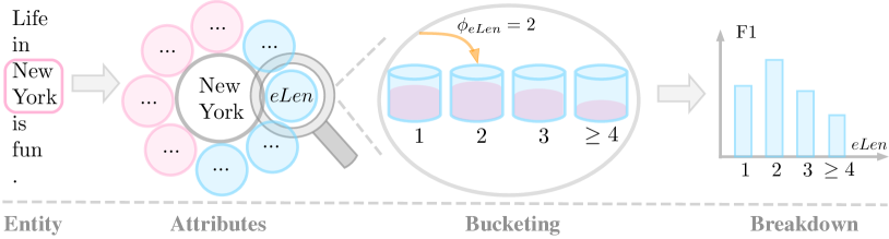
Figure 1: An example of our evaluation methodology. eLen (entity length) represents one of the attributes (detailed in Sec. 3.1) of the entity “New York”. After bucketing, performance can be broken down over different attribute values.

Orthogonally, some other works Qian et al. (2018); Hu et al. (2020); Luo et al. (2020); Li et al. (2020); Lin et al. (2020) evaluate holistic metrics such as F1 across multiple datasets that differ in domain, language, or other characteristics (Sang and De Meulder, 2003; Collobert et al., 2011; Weischedel et al., 2013). Although this enables us to more comprehensively assess the models, the reliance on holistic metrics precludes a finer-grained view of how various aspects of the model performance vary across the different settings.

In this paper, we argue that an ideal evaluation methodology should be (1) fully or partially automatic, (2) allow evaluation and comparison across multiple datasets, and (3) allow users to dig deeper into fine-grained strengths and weaknesses of each model. To this end, we devise a generalized, fine-grained, and multi-dataset evaluation methodology for the task of NER, as demonstrated in Fig. 1. Specifically, it leverages the notion of “attributes”, values which characterize the properties of an entity that may be correlated with the NER performance (e.g. entity length in words). Afterward, we partition test entities into a set of buckets based on the entity’s attributes, where entities in different buckets may have different performance scores on average (e.g. entities with more words may be predicted less accurately).

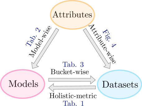
Figure 2: Relations among attributes, models, and datasets.

Methodologically, our evaluation framework allows for three analytical views as elucidated in Fig. 2. Model-wise (Sec. 5.1) analysis investigates how the performances of different models vary according to attribute value (e.g. “Is a model with a CRF layer better at dealing with long entities?”). Attribute-wise (Sec. 5.2) analysis compares how different attributes affect performance on different datasets (e.g. “Does entity length correlate with model performance on all datasets or just some?”). Bucket-wise (Sec. 5.3) compares among all possible analysis dimensions, and can diagnose the strengths and weaknesses of existing models (e.g. “What entity attributes indicate that a BERT-based model will likely fail?”), or help us understand how different choices of datasets influence model performance (e.g. “On which datasets is using a CRF layer more appropriate?”).

Experimentally, we conduct a comprehensive analysis over twelve models, eight attributes, and six datasets. Proposed quantifiable measures allow us to draw several qualitative conclusions as highlighted below: 1) label consistency (the degree of label agreement of an entity on the training set) and entity length have a consistent influence on NER task’s performance (Sec. 5.2.2); 2) CRF-based systems are more likely to make a mistake compared with MLP-based systems when dealing with long entities (Sec. 5.1.2); 3) Higher-frequency tokens of a test entity cannot guarantee better performance since other crucial factors such as label consistency also matter (Sec. 5.2.2); 4) Even more advanced models (e.g., BERT, Flair) fail to predict entities with low label consistency (Sec. 5.3.2).

Finally, motivated by observation 4), we present an effective solution to improve current NER systems. Quantitative and qualitative experiments demonstrate that introducing larger context is an effective method, obtaining improvements of up to 10 points in F1 score on some datasets.

2 Background

Task Description

NER is frequently formulated as a sequence labeling problem (Chiu and Nichols, 2015; Huang et al., 2015; Ma and Hovy, 2016; Lample et al., 2016), where $X=\{x_{1},x_{2},\ldots,x_{T}\}$ is an input sequence and $Y=\{y_{1},y_{2},\ldots,y_{T}\}$ are the output labels (e.g., “B-PER”, “I-LOC”, “O”). The goal of this task is to accurately predict entities by assigning output label $y_{t}$ for each token $x_{t}$: $P(Y|X)=P(y_{t}|X,y_{1},\cdots,y_{t-1})$

Standard Evaluation Strategy for NER

The common evaluation metric for NER systems Sang and De Meulder (2003) is to compute a corpus-level metric using micro-averaged $F1$ score: $F1=\frac{2\times P\times R}{P+R}$: where $P$ is the percentage of named entities output by learning system that are correct. $R$ is the percentage of gold entities identified by the system. Here a named entity is correct only if it is an exact match of an annotated entity.

3 Attribute-aided Evaluation

Our proposed attribute-aided evaluation methodology involves two key elements: attribute definition and bucketing. We first define diverse attributes for each entity, by which test entities are partitioned into different buckets. We then calculate the performance for each bucket of test entities.

3.1 Attribute Definition

Attributes are defined either over a span or a token and characterize the diverse properties thereof. In practice, the span will be instantiated as a genuine or a mis-predicted entity (calculating precision) in the test set, while tokens can be any token in the test corpus. We classify attributes into two categories: local attributes and aggregate attributes.

Local attributes

are calculated with respect to a span or token regarding attributes of the span/token itself, its label, or the sentence in which the span appeared. We define a token $x$ or span $\mathbf{x}$, to have a gold-standard or predicted label $y=\text{lab}(\cdot)$, which occurs in sentence $X=\text{sent}(\mathbf{x})$. We also define two functions that count the number of words outside the training set $\text{oov}(\cdot)$ and the number of entities $\text{ent}(\cdot)$ in a sequence of words. Based on this, we define several feature functions $\phi(\mathbf{x})$ that can compute different attributes of each span:

• $\phi_{\texttt{str}}(\mathbf{x})$ = $\mathbf{x}$: span surface string

• $\phi_{\texttt{label}}(\mathbf{x})=\text{lab}(\mathbf{x})$: entity span label

• $\phi_{\texttt{eLen}}(\mathbf{x})=|\mathbf{x}|$: entity span length

We additionally define feature functions over tokens $\phi(x)$:

• $\phi_{\texttt{str}}(x)$ = $x$: token surface string

• $\phi_{\texttt{label}}(x)=\text{lab}(x)$: token label

We also define several features of the underlying sentence, which can be applied to either spans $\mathbf{x}$ or tokens $x$; we show the example of applying to token $x$ below:

• $\phi_{\texttt{sLen}}(x)=|\text{sent}(x)|$: sentence length

• $\phi_{\texttt{eDen}}(x)=|\text{ent}(\text{sent}(x))|/\phi_{sLen}(x)$:
  entity density

• $\phi_{\texttt{oDen}}(x)=|\text{oov}(\text{sent}(x))|/\phi_{sLen}(x)$:
  OOV density

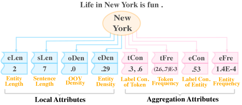
Figure 3: The eight attributes defined in this paper and corresponding values with respect to the entity “New York” in the sentence “Life in New York is fun .”. The text in orange is the full name of the attribute, in which Con. denotes Consistency.

Aggregate attributes

are properties of spans or tokens based on aggregate statistics that require calculation over the whole training corpus. To calculate these attributes, we first define $\mathcal{E}^{\text{tr}}$ as all spans/tokens in the training set. We then define an aggregation function that takes a particular span/token (example of tokens below), feature function $\phi(\cdot)$, and span set $\mathcal{E}\subseteq\mathcal{E}^{\text{tr}}$ as arguments:

$$\mathcal{F}(x,\phi(\cdot),\mathcal{E})=\frac{|\{\varepsilon|\phi(\varepsilon)=\phi(x),\forall\varepsilon\in\mathcal{E}\}|}{|\mathcal{E}|},$$ (1)

calculating the ratio of spans/tokens in $\mathcal{E}$ that have the same feature value $\phi(\cdot)$ as $x$. We can define $\mathcal{E}:=\mathcal{E}^{\text{tr}}$, calculating statistics over the entire training set. We can also choose it to be only the spans/tokens with a particular surface form:

$$\mathcal{E}^{x}:=\{\varepsilon|\phi_{\texttt{str}}(\varepsilon)=\phi_{\texttt{str}}(x),\varepsilon\in\mathcal{E}^{\text{tr}}\}.$$ (2)

Based on the above general formulation, we defined a few specific instantiations that we use in the following experiments. First, entity frequency and token frequency:

$$\phi_{\texttt{eFre}}(\mathbf{x}) :=\mathcal{F}(\mathbf{x},\phi_{\texttt{str}}(\cdot),\mathcal{E}^{\text{tr}})$$ (3)

$$\phi_{\texttt{tFre}}(x) :=\mathcal{F}(x,\phi_{\texttt{str}}(\cdot),\mathcal{E}^{\text{tr}})$$ (4)

Besides, we use two consistency-based attributes, which attempt to measure how consistently a particular span/token is labeled with a particular label:

$$\phi_{\texttt{eCon}}(\mathbf{x}) :=\mathcal{F}(\mathbf{x},\phi_{\texttt{label}}(\cdot),\mathcal{E}^{\text{tr}})$$ (5)

$$\phi_{\texttt{tCon}}(x) :=\mathcal{F}(x,\phi_{\texttt{label}}(\cdot),\mathcal{E}^{\text{tr}})$$ (6)

We give an example to illustrate above by setting $\mathbf{x}=$ “New York” with gold label “LOC”. Therefore, the numerator of $\phi_{eCon}$ tallies entities “New York” with label “LOC” in training set, while the denominator counts spans “New York”. The overall ratio quantifies the degree of label consistency in train set for a given span “New York”.

3.2 Bucketing

Bucketing is an operation that breaks down the holistic performance into different categories Neubig et al. (2019); Fu et al. (2020b). This can be achieved by dividing the set of test entities into different subsets of test entities (regarding span- and sentence-level attributes) or test tokens (regarding token-level attributes). Here we describe the entity-based bucketing strategies, which can also be similarly applied to token-based strategies. The bucketing process can be expressed in the following general form:

$$\mathcal{E}_{1}^{te},\cdots,\mathcal{E}_{m}^{te}=\mathrm{Bucket}(\mathcal{E}^{te},\phi(\cdot))$$ (7)

where $\mathcal{E}^{te}$ represents a set of test entities or tokens, and $m$ is the number of buckets. $\phi(\cdot)$ denotes one type of feature functions (as defined in Sec. 3.1) to calculate attribute value for a given entity (e.g., $\phi_{\texttt{eLen}}(\mathbf{x})$ to compute span length).

Specifically, we divide the range of attribute values into $m$ discrete parts, whose intervals can be obtained mainly based on two ways: 1) dividing value range evenly 2) dividing test entities or tokens equally. In practice, the way to obtain intervals may be diverse for different attributes. We detail our settings in the appendix. Finally, once we have generated buckets, we calculate the F1 score with respect to entities (or tokens) of each bucket. We can easily extend the attribute-aided evaluation to other tasks, such as Chinese Word Segmentation Fu et al. (2020a).

4 Experimental Settings

Models	Char/Subword					Word			Sentence		Decoder		Overall F1
	none	cnn	elmo	flair	bert	none	rand	glove	lstm	cnn	crf	mlp	CoNLL	WNUT	BN	BC	MZ	WB
CRF++													80.74	21.53	82.02	67.71	77.80	47.90
CnonWrandLstmCrf	$\surd$						$\surd$		$\surd$		$\surd$		78.13	17.24	80.36	66.17	73.89	49.80
CcnnWnoneLstmCrf		$\surd$				$\surd$			$\surd$		$\surd$		77.01	22.73	77.96	65.01	79.05	47.31
CcnnWrandLstmCrf		$\surd$					$\surd$		$\surd$		$\surd$		83.80	22.57	83.59	71.57	78.85	52.14
CcnnWgloveLstmCrf		$\surd$						$\surd$	$\surd$		$\surd$		90.48	40.61	86.78	76.04	85.39	60.17
CcnnWgloveCnnCrf		$\surd$						$\surd$		$\surd$	$\surd$		90.14	36.21	86.42	76.74	88.10	49.10
CcnnWgloveLstmMlp		$\surd$						$\surd$	$\surd$			$\surd$	88.05	32.84	84.07	70.00	81.09	56.61
CelmWnoneLstmCrf			$\surd$			$\surd$			$\surd$		$\surd$		91.64	44.56	89.75	77.10	86.32	60.51
CelmWgloveLstmCrf			$\surd$					$\surd$	$\surd$		$\surd$		92.22	45.33	89.35	78.71	85.70	63.26
CbertWnoneLstmMlp					$\surd$	$\surd$			$\surd$			$\surd$	91.11	47.77	89.64	81.03	86.90	66.35
CflairWnoneLstmCrf				$\surd$		$\surd$			$\surd$		$\surd$		89.98	41.49	87.98	77.46	84.11	56.71
CflairWgloveLstmCrf				$\surd$				$\surd$	$\surd$		$\surd$		93.03	45.96	87.92	77.23	85.56	63.38

Table 1: Neural NER systems with different architectures. CRF++ is a Conditional Random Fields Lafferty et al. (2001) method based on feature engineering. Bold is the best performance of a given dataset according to F1. For the model name, “C” refers to “Char/Subword” and “W” refers to “Word”. For example, ”CnonWrandLstmCrf” is a model with no character features, with randomly initialized embeddings, and the sentence encoder is LSTM and decoder is CRF.

In this section we describe our experimental settings, each of which is followed by an experiment and analysis results.

4.1 NER Datasets for Evaluation

We conduct experiments on: CoNLL-2003 (CoNLL),  WNUT-2016 (WNUT), and OntoNotes 5.0 dataset.  The CoNLL dataset (Sang and De Meulder, 2003) is based on Reuters data (Collobert et al., 2011). The WNUT dataset (Strauss et al., 2016) is provided by the second shared task at WNUT-2016 and consists of social media data from Twitter. The OntoNotes 5.0 dataset (Weischedel et al., 2013) is collected from broadcast news (BN), broadcast conversation (BC), weblogs (WB), and magazine genre (MZ).

4.2 Models

We varied the evaluated models mainly in terms of four aspects: 1) character/subword-sensitive encoder: ELMo (Peters et al., 2018), Flair (Akbik et al., 2018, 2019), BERT  (Devlin et al., 2018)

2) additional word embeddings: GloVe (Pennington et al., 2014); 3) sentence-level encoders: LSTM (Hochreiter and Schmidhuber, 1997), CNN (Kalchbrenner et al., 2014; Chen et al., 2019); 4) decoders: MLP or CRF (Lample et al., 2016; Collobert et al., 2011). In total, we study 12 NER models and we give more detailed description of models in the appendix. Detailed model settings are illustrated in Tab.1. We use the result from the model with the best development set performance, terminating training when the performance on development is not improved in 20 epochs.

4.3 Holistic Analysis

Before giving a fine-grained analysis, we present the results of different models on different datasets as traditional multi-dataset evaluation does. As Tab. 1 demonstrates, there is no one-size-fits-all model; different models get the best results on different datasets. Naturally, this raises the following questions: 1) what factors of the datasets significantly influence NER performance? 2) how do these factors influence the choices of models? 3) does a worse-ranked model outperform the best-ranked model in some aspects and how do datasets influence the choices of models? The following analyses will investigate these questions.

5 Fine-grained Analysis

To better characterize the relationship among models, attributes, and datasets, we propose three analysis approaches: model-, attribute-, and bucket-wise.

Formally, we refer to $M=\{m_{1},\cdots,m_{|M|}\}$ as a set of models and $\Phi=\{\phi_{1},\cdots,\phi_{|\Phi|}\}$ as a set of attributes. As described in Sec. 3.2, the test set $\mathcal{E}$ could be split into different buckets of $\mathcal{E}=\{\mathcal{E}^{j}_{1},\cdots,\mathcal{E}^{j}_{|\mathcal{E}|}\}$ based on an attribute $\phi_{j}$. We introduce the concept of a performance table $\mathcal{T}\in\mathbb{R}^{|M|\times|\Phi|\times|\mathcal{E}|}$, whose element $\mathcal{T}_{ijk}$ represents the performance ($F1$ score) of $i$-th model on the $k$-th sub-test set (bucket) generated by $j$-th attribute. Next, we will explain how above-mentioned analysis approaches are defined based on $\mathcal{T}$.

		Spearman ($\mathbf{S}^{\rho}_{i,j}$)								Standard Deviation ($\mathbf{S}^{\sigma}_{i,j}$)
Model	F1	eDen	oDen	sLen	eCon	tCon	eFre	tFre	eLen	eDen	oDen	sLen	eCon	tCon	eFre	tFre	eLen
CRF++	55.00	-4	9	-10	87	79	96	56	-92	5.5	7.5	5.2	16.2	12.7	14.8	6.6	5.8
CnonWrandLstmCrf	60.93	-37	-2	-7	90	79	94	57	-92	5.9	8.2	4.4	21.2	16.3	21.3	9.9	7.8
CcnnWnoneLstmCrf	61.51	-11	-6	-7	77	85	95	49	-75	6.1	6.7	5.6	15.2	11.9	14.3	5.9	7.2
CcnnWrandLstmCrf	65.42	-19	5	-7	87	82	95	44	-92	5.5	7.3	4.0	16.0	12.5	15.5	6.6	8.8
CcnnWgloveLstmCrf	73.25	-23	2	-15	90	64	93	12	-92	5.7	6.6	4.0	12.0	9.2	14.9	5.2	9.0
CcnnWgloveCnnCrf	75.52	-16	-11	-25	90	65	88	0	-83	5.6	6.8	3.8	12.4	9.6	14.7	6.1	9.0
CcnnWgloveLstmMlp	68.78	-34	5	-17	93	63	97	3	-67	5.9	6.8	3.9	14.9	11.6	16.5	6.8	7.1
CelmWnoneLstmCrf	74.99	7	3	5	87	56	98	16	-83	5.8	6.6	4.1	11.5	8.5	13.6	4.9	6.5
CelmWgloveLstmCrf	75.76	-3	-8	-9	87	60	93	-2	-92	5.5	6.8	4.0	11.4	8.2	13.4	5.1	6.4
CbertWnoneLstmMlp	76.26	0	-12	0	83	56	87	17	-58	5.4	5.6	3.7	11.8	8.3	12.5	5.8	4.8
CflairWnoneLstmCrf	72.96	-25	7	-23	80	72	97	21	-83	5.6	6.4	4.1	12.2	9.1	13.6	5.3	6.6
CflairWgloveLstmCrf	75.51	-16	-11	8	87	67	91	24	-92	5.2	5.8	4.0	11.6	8.7	13.1	5.3	6.5

Table 2: Model-wise measures (Percentage) $\mathbf{S}^{\rho}_{i,j}$ and $\mathbf{S}^{\sigma}_{i,j}$ which are the average over all the datasets. The F1 score for a model is also an average case on all the datasets. The value in grey denotes the attribute does not pass a significance test ($p\geq 0.05$). The values in green and in pink support observation 1 and observation 2, respectively. The bold is the maximum value in the attribute column.

5.1 Exp-I: Model-wise Analysis

Model-wise analysis investigates how different attributes influence performance of models with different architectures and initializations, e.g. “does eLen influence performance of a CNN-LSTM-CRF-based NER system?”

5.1.1 Approach

Here we adopt two types of statistical variables $\mathbf{S}^{\rho}_{i,j}$ and $\mathbf{S}^{\sigma}_{i,j}$ to characterize how the $j$-th attribute influences the of performance $i$-th model.

$$\mathbf{S}^{\rho}_{i,j} =\mathrm{Spearman}(\mathcal{T}[i,j:],R_{j})$$ (8)

$$\mathbf{S}^{\sigma}_{i,j} =\mathrm{Std}(\mathcal{T}[i,j:])$$ (9)

where $\mathrm{Spearman}$ is a function to calculate the Spearman’s rank correlation coefficient (Mukaka, 2012) and $R_{j}$ is the rank values of buckets based on the $j$-th attribute. $\mathrm{Std}(\cdot)$ is the function to compute the standard deviation.

Intuitively, $\mathbf{S}^{\rho}_{i,j}$ characterizes how well the performance of the $i$-th model correlates with the values of the $j$-th attribute while $\mathbf{S}^{\sigma}_{i,j}$ measures the degree to which this attribute influences the model’s performance. For example, $\mathbf{S}^{\rho}_{CNN,\texttt{eCon}}=0.9$ reveals that the performance of the CNN model positively and highly correlates with the attribute value eCon (label consistency). And a larger $\mathbf{S}^{\sigma}_{CNN,\texttt{eCon}}$ implies that CNN model’s performance is heavily influenced by the factor eCon.

Significance Tests: We perform Friedman’s test Zimmerman and Zumbo (1993) with $p=0.05$. We examine whether the performance of different buckets partitioned by an attribute have the same expected performance, and the significance testing results are shown in appendix. We omit the attributes whose $\mathbf{S}^{\rho}_{i,j}$ and $\mathbf{S}^{\sigma}_{i,j}$ are not statistically significant (the values in grey in Tab. 2).

5.1.2 Observations

Tab. 2 illustrates the average case of $\mathbf{S}^{\rho}_{i,j}$ and $\mathbf{S}^{\sigma}_{i,j}$ on all datasets. We highlight some major observations and more are in the appendix.

1) The performance of character-unaware models is more sensitive to the label consistency. We observe that the performances of CRF++ and CnonWrandLstmCrf are highly correlated with eCon, and tCon with high values of $\mathbf{S}^{\rho}$ and $\mathbf{S}^{\sigma}$. Specifically, CcnnWrandLstmCrf achieve higher performance and lower $\mathbf{S}^{\sigma}$ than CnonWrandLstmCrf. This suggests that the character-level encoder plays a major role in generalization to entities with low label consistency.

2) The influence of entity length varies greatly between different decoders. Entity length is strongly negatively correlated with the performance of models, which means the performance of the model will drop with the entity length increasing. We observe that the variance scores $S^{\sigma}$ of CcnnWgloveLstmMlp and CbertWnoneLstmMlp are the smallest, compared with the variances of the models using non-contextualized and contextualized pre-trained embeddings, respectively. We attribute this to the structural biases of different decoders: MLP-based models have better robustness when dealing with long entities, while CRF-based models may lead to error propagation. We will present a detailed explanation of this in Sec. 5.3.2.

5.2 Exp-II: Attribute-wise Analysis

Attribute-wise analysis aims to quantify the degree to which an attribute influences NER performance overall, across all systems.

5.2.1 Approach

To achieve this, we introduce two dataset bias measures: task-independent variable $\zeta_{j}$ and task-dependent variable $\rho_{j}$ based on Eq. 8:

$$\zeta_{j}(\mathcal{E},\phi(\cdot)) =\frac{1}{N}\sum_{i}^{N}\phi_{j}(\mathbf{x}),$$ (10)

$$\rho_{j} =\frac{1}{|M|}\sum_{i}^{|M|}|\mathbf{S}^{\rho}_{i,j}|,$$ (11)

where $\mathcal{E}$ denotes a dataset, $\phi_{j}(\mathbf{x})$ is the feature function to calculate an attribute value for a given entity $\mathbf{x}$, $j$ denotes the $j$-th attribute function, and $N$ and $|M|$ are the numbers of test entities and models respectively.

For example, when $j$ denotes the attribute of sentence length, $\zeta_{j}$ is the average sentence length of the whole dataset. Intuitively, a higher absolute value of $\rho_{j}$ suggests that attribute $j$ is a crucial factor, whose values heavily correlate with the performances of NER systems.

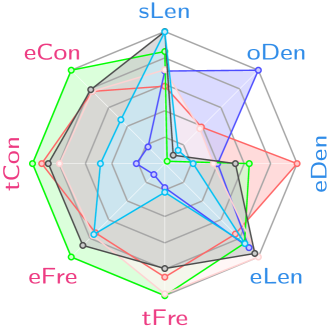
(a) $\zeta$

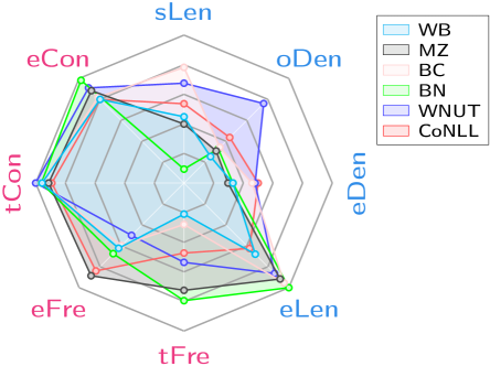
(b) $\rho$

Figure 4: Dataset biases characterized by measures $\zeta$ and $\rho$. We normalize $\zeta$ on each attribute by dividing the maximum $\zeta$ on six datasets, and $\rho\in[0,1]$.

5.2.2 Observations

Similar to the above section, we conduct Friedman’s test at $p=0.05$. For all attributes, we find different-valued buckets are significantly different in their expected performance ($p<0.05$). We include a full version of $p$ values in the appendix. Detailed observations are listed as follows:

1) Label consistency and entity length have a more consistent influence on NER performance. The common parts of the radar chart in Fig. 4(b) illustrate that for all datasets, the performance of the NER task is highly correlated with these attributes: tCon (label consisency of tokens), eCon (label consistency of entities), eLen (entity length). This reveals that the prediction difficulty of a named entity is commonly influenced by label consistency (tCon, eCon) and entity length (eLen).

2) Frequency and sentence length matter but are minor factors. The outliers in the radar chart highlight the peculiarities of different datasets. Intuitively, in Fig. 4(b), on these attributes: sLen, tFre, oDen, the extent to which different datasets are affected varies greatly, and thus these attributes are not, in general, decisive factors for the NER task. Typically, as observed from Fig. 4(b), Spearman correlations of $\rho$ on the attribute tFre vary greatly, i.e., a smaller $\rho$ on BC and WB. This implies that tFre is not a decisive factor and higher-frequency tokens cannot guarantee better performance since other crucial factors such as label consistency also matter. We print the performance of the buckets with respect to token frequency, and find that the bucket with higher token frequency does not achieve a better performance.

Understanding these intrinsic differences in datasets provides us with evidence to explain how different datasets may influence different choices of models, which will be elaborated later (Sec. 5.3).

CoNLL03

WNUT16

OntoNotes-MZ

OntoNotes-BC

OntoNotes-BN

OntoNotes-WB

eDen

oDen

sLen

eCon

eFre

tCon

tFre

eLen

eDen

oDen

sLen

eCon

eFre

tCon

tFre

eLen

eDen

oDen

sLen

eCon

eFre

tCon

tFre

eLen

eDen

oDen

sLen

eCon

eFre

tCon

tFre

eLen

eDen

oDen

sLen

eCon

eFre

tCon

tFre

eLen

eDen

oDen

sLen

eCon

eFre

tCon

tFre

eLen

Overall F1

M1: 91.11

M1: 47.77

M1: 86.90

M1: 81.03

M1: 89.64

M1: 66.35

M1: CbertWnoneLstmMlp

Self-diagnosis

Overall F1

M1: 90.48; M2: 88.05

M1: 40.61; M2: 32.84

M1: 85.39; M2: 81.09

M1: 76.04; M2: 70.00

M1: 86.78; M2: 84.07

M1: 60.17; M2: 56.61

M1: CcnnWgloveLstmCrf

M2: CcnnWgloveLstmMlp

Comparative diagnosis

Table 3: Self-diagnosis, and Comparative diagnosis (Sec. 5.3.1) of different NER systems. M1 and M2 denote two models. We classify the attribute values into four categories: extra-small (XS), small (S), large (L) and extra-large (XL). In the self-diagnosis histogram, green (red) $x$ ticklabels represents the bucket value of a specific attribute on which system achieved best (worst) performance. Gray bins represent worst performance while blue bins denote the gap between best and worst performance. In the comparative diagnosis histogram, green (red) $x$ ticklabels represents the bucket value of a specific attribute on which system M1 surpasses (under-performs) M2 by the largest margin that is illustrated by a green (red) bin.

5.3 Exp-III: Bucket-wise Analysis

Bucket-wise analysis aims to identify the buckets that satisfy some specific constraints. In this paper, we present two flavors of diagnostic: self-diagnosis and comparative diagnosis.

5.3.1 Approach

Self-diagnosis

Given a model $M_{1}$ and a specific evaluation attribute (e.g., eLen), self-diagnosis selects the buckets in which test samples have achieved the highest and lowest performance (F1 score). Intuitively, this operation can help us diagnose under which conditions a particular model performs well or poorly: $\mathrm{SelfDiag}(M_{1})=\mathrm{argFunc}_{k}\mathcal{T}[M_{1},j,k]$ where $\mathrm{argFunc}$ can be instantiated as $\mathrm{argMax}$ and $\mathrm{argMin}$.

Comparative diagnosis

Given two models $M_{1}$, $M_{2}$ and an attribute, comparative diagnosis aims to select buckets in which the performance gap between the two systems achieve the highest and lowest values. This method can indicate under which conditions a particular system may have a relative advantage over another system: $\mathrm{CoDiag}(M_{1},M_{2})=\mathrm{argFunc}_{k}(\mathcal{T}[M_{1},j,k]-\mathcal{T}[M_{2},j,k])$

Significance Tests

We test for statistical significance at $p=0.05$ with Wilcoxon’s signed-rank test (Wilcoxon et al., 1970). The null hypothesis is that, given a specific attribute value (e.g. long entities eLen:XL), two different models have the same expected performance.

5.3.2 Self-Diagnosis

BERT

The first row in Tab. 3 illustrates the self-diagnosis of the model CbertWnonelstmMlp. The green (red) $x$ ticklabels represent the bucket value of a specific attribute on which system has achieved best (worst) performance. Gray bins represent worst performance while blue bins denote the gap between best and worst performance.

We observe that large performance gaps (tall blue bins) commonly occur for the attributes label consistency and entity frequency, and the worst performance on these attributes was obtained on buckets with low consistency (eCon, tCon:XS/S) and low entity frequency (eFre:S).

We conduct significance testing on the worst and best performances of eCon ($1.7\times 10^{-8}$), tCon ($2.3\times 10^{-7}$) and eFre ($1.2\times 10^{-5}$) respectively, and they all passed with $p<0.05$. This reveals that it is still challenging for contextualized pre-trained NER systems to handle entities with lower label consistency and lower entity frequency.

5.3.3 Comparative Diagnosis

We highlight major observations and include more analysis in the appendix.

CRF v.s. MLP

The benefits of using CRF on the sentence with high entity density (eDen:XL) are remarkably stable, and improvement can be seen in all datasets ($p=1.8\times 10^{-5}<0.05$). Similarly, based on attribute-wise metric $\zeta$ in Fig. 4(a), we find label consistency (eCon, tCon) is a major factor for the choices of CRF and MLP layers:

1) Introducing a CRF achieves larger improvements on long entities once the dataset has a lower label consistency (e.g. $\zeta_{\texttt{eCon},\texttt{tCon}}$(WNUT), $\zeta_{\texttt{eCon},\texttt{tCon}}$(WB), and $\zeta_{\texttt{eCon},\texttt{tCon}}$(BC) are lowest). We conduct the significance testing on CRF and MLP systems with respect to the long entities on these three datasets (WNUT, WB, and BC), and the result indicates that the performance of the CRF and MLP systems are significantly different on long entity bucket ($p=6.5\times 10^{-4}<0.05$). 2) by contrast, if a dataset has a higher label consistency ($\zeta_{\texttt{eCon},\texttt{tCon}}$(CoNLL),$\zeta_{\texttt{eCon},\texttt{tCon}}$(BN), $\zeta_{\texttt{eCon},\texttt{tCon}}$(MZ) are highest), using the CRF layer does not exhibit significant gains (even worse than models without CRF) on longer entities (eLen:XL). We do significance testing like 1), and $p=5.1\times 10^{-3}<0.05$.

6 Application: Well-grounded Model Improvement

The purpose of interpretable evaluation and analysis is to provide more evidence for us to rethink current learning models and move forward. In what follows, we choose a piece of evidence observed from the above analysis and attempt to present one simple solution to improve the model. From Sec. 5.2 and Sec. 5.3.2, we know that label consistency is a decisive factor, and even more advanced models (e.g., BERT, Flair) fail to consistently predict entities with low label consistency. An intuitive idea to disambiguate these entities is using more contextual information. To this end, we shift the setting of traditional sentence-level training and testing to use larger context, and investigate this change’s effectiveness.

6.1 Experimental Setting

We choose CbertWnoneLstmMlp as a base model, which will be trained under different numbers ($K=1,2,3,4,5,6,10$) of contextual sentences on all six datasets respectively. For example, $K=2$ represents that each training sample is constructed by concatenating two consecutive sentences from the original dataset ($K=1$).

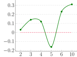
(a) CoNLL

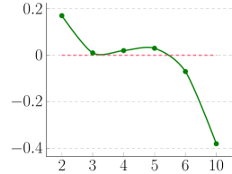
(b) BN

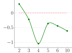
(c) MZ

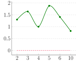
(d) BC

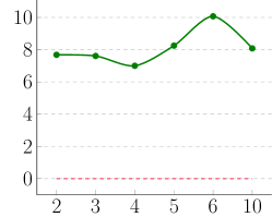
(e) WB

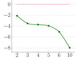
(f) WNUT

Figure 5: Illustration of the improvement achieved by the larger context method with different sizes ($K$) on different datasets. The part above the red suggests the improvement brought by the corresponding value of $K$.

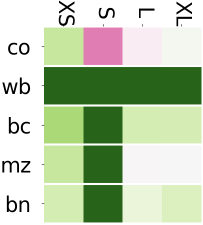
(a) eCon

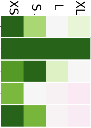
(b) tCon

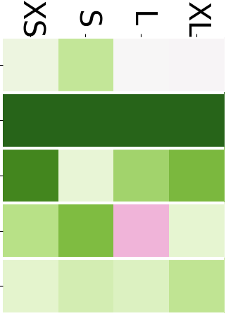
(c) eFre

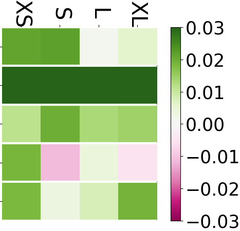
(d) tFre

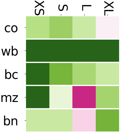
(e) eDen

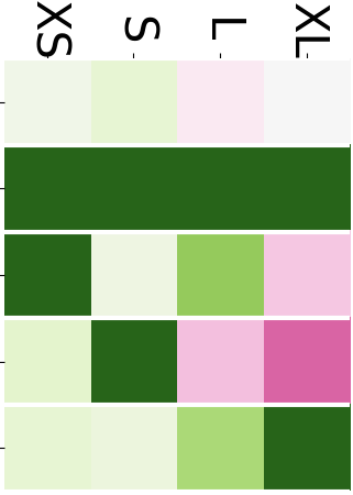
(f) eLen

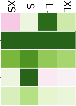
(g) sLen

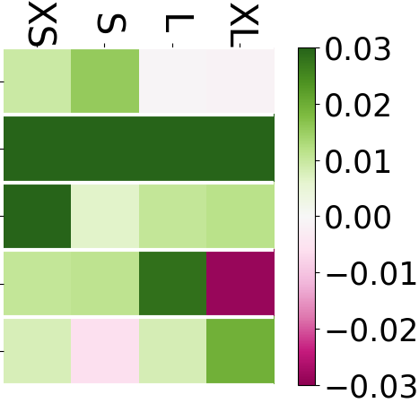
(h) oDen

Figure 6: The relative increase of the larger-context method on five datasets based on eight evaluation attributes. “Co” represents the dataset CoNLL-2003 while “wb”, “bc”, “mz”, “bn” denote different domains from the OntoNotes.

6.2 Results and Analysis

Results

As presented in Fig. 5, the green line describes the relative improvement of the larger context method compared with the vanilla model ($K=1$) with different numbers of context sentences $K=2,\cdots,10$. In detail, we observed:

1) For most of the datasets (except “WNUT”), the performance increases as more context sentences are introduced. 2) Surprisingly, we achieved a 10.07 improvement ($66.35$ vs. $76.42$, significance testing result: $p=5.1\times 10^{-3}<0.05$) F1 score on dataset “WB”, with such a simple larger-context training method. 3) There is no gain on “WNUT”, and the reason can be attributed to lack of dependency between samples, which are collected from Twitter where each sentence is relatively independent with the another.

Analysis using Multi-dimensional Evaluation

To probe into where the gain afforded by larger context comes from, we use our proposed evaluation attributes to conduct a fine-grained investigation, aiming to answer the question: how does this method influence different datasets’ performance seen from different attributes? (e.g., label consistency of entity, eCon). As expressed in Fig. 13, the value of each unit in the heat maps denotes the relative increase achieved by the larger-context method. Intuitively, a darker green area implies more significant improvement while a darker red unit suggests larger-context leads to worse performance.

Different evaluation attributes allow us to understand the source of improvement from diverse perspectives: 1) in terms of label consistency (eCon, tCon), test entities with lower label consistency will achieve larger improvements with the help of more contextual sentences. Importantly, from Fig. 13 we can see this observation holds true for all datasets. 2) in terms of entity length (eLen), larger-context information has no advantage in dealing with longer entities (L, XL). For example, in the three of five datasets, more contextual sentences lead to worse performance on longer test entities.

7 Discussion

This paper has provided a framework where we can covert our understanding of the NER task (i.e., which attributes matter for the current task?) into interpretable evaluation aspects, and define axes through which we can apply them to acquire insights and make model improvements. This is just a first step towards the goal of fully-automated interpretable evaluation, and applications to new attributes and tasks beyond NER are promising future directions.

Appendix A Models Description

Tab. 1 shows the evaluated models in this paper, mainly in terms of four aspects: 1) character/subword-sensitive encoder: ELMo, Flair, BERT 2) additional word embeddings: GloVe; 3) sentence-level encoders: LSTM, CNN; 4) decoders: MLP or CRF.

For example, 1) ”CnonWrandlstmCrf” is a model with no character features, with randomly initialized embeddings, and the sentence encoder is LSTM and the decoder is CRF. 2) ”CbertWnoneLstmMlp” is a model that concatenates the representations from BERT and GloVe as a subword-sensitive encoder. Then the concatenation will be fed into an MLP layer, predicting a label over all classes. 3) ”CelmWgloveLstmCrf” is a model that concatenates the representations from ELMo and GloVe as a subword-sensitive encoder. Then the concatenation will be fed into an LSTM layer, followed by the CRF layer.

Appendix B Bucketing Interval Strategy

In this section, we will illustrate the bucketing interval with respect to attribute. We divide the range of attribute values into $m$ discrete parts. For a given attribute, the number of entities covered by an attribute value is various. For example, oDen=0 covered nearly half of the entity in the test set for OOV density; for label consistency, eCon=0 and eCon=1 each occupy a large part of the test entities. We customize the interval method for each attribute in accordance with its own characteristics.

1) Label consistency (eCon, tCon): first, we divide the entities in the test set with attribute values $\phi_{eCon}(\mathbf{x})=0$ and $\phi_{eCon}(\mathbf{x})=1$ into the first bucket ($\mathcal{E}_{1}^{te}$) and last bucket $\mathcal{E}_{m}^{te}$, respectively; then, divide the remaining entities equally into $m-2$ buckets. The bucketing interval strategy of eCon is suitable for tCon.

2) Frequency (eFre, tFre) and OOV density (oDen): first, we divide the entities in test set with attribute value $\phi_{eFre}(\mathbf{x})=0$ into the first bucket ($\mathcal{E}_{1}^{te}$); then, divide the remaining entities equally into $m-1$ buckets. The bucketing interval strategy of eFre is suitable for tFre and oDen.

3) Sentence length (sLen) and entity density (eDen): we divide the test entities equally into $m$ buckets.

4) Entity length (eLen): a small $m$ is suitable for entity length, because of a few attribute values (generally, the entity length is rarely greater than 6). In this paper, we put the entities in the test set with lengths of 1, 2, 3, and $\geq 4$ into four buckets, respectively.

	CoNLL03									WNUT16									OntoNotes-MZ									OntoNotes-BC									OntoNotes-BN									OntoNotes-WB
		eDen	oDen	sLen	eCon	eFre	tCon	tFre	eLen		eDen	oDen	sLen	eCon	eFre	tCon	tFre	eLen		eDen	oDen	sLen	eCon	eFre	tCon	tFre	eLen		eDen	oDen	sLen	eCon	eFre	tCon	tFre	eLen		eDen	oDen	sLen	eCon	eFre	tCon	tFre	eLen		eDen	oDen	sLen	eCon	eFre	tCon	tFre	eLen
Overall F1	M1: 90.48; M2: 90.14									M1: 40.61; M2: 36.21									M1: 85.39; M2: 88.10									M1: 76.04; M2: 76.74									M1: 86.78; M2: 86.42									M1: 60.17; M2: 49.10
M1: CcnnWgloveLstmCrf
M2: CcnnWgloveCnnCrf
Comparative diagnosis
Overall F1	M1: 93.03; M2: 92.22									M1: 45.96; M2: 45.33									M1: 85.56; M2: 85.70									M1: 77.23; M2: 78.71									M1: 87.92; M2: 89.35									M1: 63.38; M2: 63.26
M1: CflairWgloveLstmCrf
M2: CelmWgloveLstmCrf
Comparative diagnosis

Table 4: Comparative diagnosis of different NER systems. M1 and M2 denote two models. We classify the attribute values into four categories: extra-small (XS), small (S), large (L), and extra-large (XL). In the comparative diagnosis histogram, green (red) $x$ ticklabels represents the bucket value of a specific attribute on which system M1 surpasses (under-performs) M2 by the largest margin that is illustrated by a green (red) bin.

Appendix C Model-wise Analysis and Observation

Tab. 2 gives the model-wise measures $\mathbf{S}^{\rho}_{i,j}$ and $\mathbf{S}^{\sigma}_{i,j}$ which are the average case on all the datasets. We find that: pre-trained knowledge enhanced models are tardier to the token-level attribute. We observe that the values of $\mathbf{S}^{\rho}$ dropped sharply on tCon and tFre, when the pre-trained embedding is introduced, therefore, comparing with the models without pre-trained knowledge, the performance of the models with pre-trained knowledge is slower improved as the increasing of token consistency and token frequency. Specifically, the models with pre-trained knowledge have higher performance and lower $\mathbf{S}^{\sigma}$, compared with the models without pre-trained knowledge. This reveals that the introduction of external knowledge will handle the lower label consistency of token and low token frequency.

dataset	eDen	oDen	sLen	eCon	eFre	tCon	tFre	eLen
conll03	${2.2\times 10^{-12}}$	${2.0\times 10^{-17}}$	${1.1\times 10^{-10}}$	${1.0\times 10^{-6}}$	${1.2\times 10^{-14}}$	${8.8\times 10^{-18}}$	${8.2\times 10^{-11}}$	${4.8\times 10^{-7}}$
wnut16	${2.6\times 10^{-15}}$	${7.3\times 10^{-17}}$	${1.1\times 10^{-13}}$	${1.4\times 10^{-6}}$	${4.8\times 10^{-10}}$	${3.7\times 10^{-15}}$	${1.4\times 10^{-14}}$	${4.8\times 10^{-7}}$
notewb	${3.9\times 10^{-16}}$	${9.0\times 10^{-13}}$	${5.5\times 10^{-09}}$	${7.5\times 10^{-8}}$	${2.1\times 10^{-16}}$	${2.1\times 10^{-18}}$	${8.0\times 10^{-17}}$	${3.6\times 10^{-7}}$
notemz	${3.6\times 10^{-11}}$	${5.1\times 10^{-11}}$	${2.2\times 10^{-11}}$	${1.3\times 10^{-6}}$	${5.3\times 10^{-12}}$	${2.9\times 10^{-18}}$	${6.1\times 10^{-16}}$	${5.5\times 10^{-7}}$
notebc	${1.7\times 10^{-05}}$	${3.8\times 10^{-11}}$	${8.8\times 10^{-13}}$	${1.3\times 10^{-6}}$	${6.3\times 10^{-15}}$	${4.1\times 10^{-18}}$	${5.2\times 10^{-15}}$	${5.5\times 10^{-7}}$
notebn	${2.9\times 10^{-07}}$	${1.6\times 10^{-11}}$	${5.7\times 10^{-14}}$	${1.3\times 10^{-7}}$	${2.9\times 10^{-15}}$	${2.9\times 10^{-18}}$	${2.4\times 10^{-15}}$	${7.5\times 10^{-8}}$

Table 5: $p$-values from the Friedman test. The null hypothesis is that the performance of different buckets with respect to an attribute has the same means for a given dataset.

Appendix D Bucket-wise Analysis and Observation

Tab. 4 illustrates the comparative diagnosis of different NER systems. Here, we will give the observations.

LSTM v.s. CNN

The sentence encoder of CNN is better at dealing with long entities (eLen:XL) on the datasets with a high value of $\zeta_{eCon}$. As shown in Tab.4, the performance of LSTM and CNN systems are significantly different on the “eLen:XL” bucket ($p=1.2\times 10^{-2}<0.05$) without regard to WNUT16 and WB two datasets which have the lowest values of $\zeta_{eCon}$.

The encoder of LSTM does better in dealing with highly-ambiguous entities (eCon:S). For example, the LSTM system has surpassed CNN on the datasets WNUT and WB, whose average label ambiguities of entities are the two largest ones.

Model	eDen	oDen	sLen	eCon	eFre	tCon	tFre	eLen
CRF++	0.39	0.31	0.28	$9.4\times 10^{-4}$	$1.8\times 10^{-3}$	$9.4\times 10^{-4}$	$9.7\times 10^{-3}$	$3.8\times 10^{-3}$
CnoneWrandLstmCrf	0.09	0.17	0.10	$1.0\times 10^{-3}$	$1.0\times 10^{-3}$	$9.4\times 10^{-4}$	$1.8\times 10^{-3}$	$3.8\times 10^{-3}$
CcnnWnoneLstmCrf	0.10	0.80	0.80	$3.2\times 10^{-3}$	$9.4\times 10^{-4}$	$1.5\times 10^{-3}$	$2.9\times 10^{-2}$	$5.6\times 10^{-3}$
CcnnWrandLstmCrf	0.46	0.56	0.85	$2.2\times 10^{-3}$	$7.1\times 10^{-4}$	$9.4\times 10^{-4}$	$1.8\times 10^{-3}$	$3.8\times 10^{-3}$
CcnnWgloveLstmCrf	0.61	0.28	0.49	$1.5\times 10^{-3}$	$5.6\times 10^{-3}$	$1.1\times 10^{-3}$	$9.7\times 10^{-3}$	$1.5\times 10^{-3}$
CcnnWgloveCnnCrf	0.61	0.39	0.80	$1.5\times 10^{-3}$	$6.3\times 10^{-3}$	$1.7\times 10^{-3}$	$1.5\times 10^{-3}$	$2.0\times 10^{-3}$
CcnnWgloveLstmMlp	0.39	0.46	0.33	$1.1\times 10^{-3}$	$2.9\times 10^{-3}$	$1.1\times 10^{-3}$	$5.6\times 10^{-3}$	$6.7\times 10^{-3}$
CelmoWnoneLstmCrf	0.26	0.57	0.33	$2.0\times 10^{-3}$	$4.2\times 10^{-3}$	$1.1\times 10^{-3}$	$5.6\times 10^{-3}$	$5.6\times 10^{-3}$
CelmoWgloveLstmCrf	0.85	0.10	0.22	$2.0\times 10^{-3}$	$3.8\times 10^{-3}$	$1.1\times 10^{-3}$	$8.1\times 10^{-3}$	$1.5\times 10^{-3}$
CbertWnonLstmMlp	0.06	0.12	0.61	$3.8\times 10^{-3}$	$4.2\times 10^{-3}$	$2.0\times 10^{-3}$	$2.0\times 10^{-2}$	$3.5\times 10^{-2}$
CflairWnoneLstmCrf	0.13	0.22	0.39	$2.2\times 10^{-3}$	$3.8\times 10^{-3}$	$1.1\times 10^{-3}$	$3.8\times 10^{-3}$	$5.6\times 10^{-3}$
CflairWgloveLstmCrf	0.39	0.33	0.20	$4.6\times 10^{-3}$	$2.2\times 10^{-3}$	$1.1\times 10^{-3}$	$6.0\times 10^{-2}$	$3.8\times 10^{-3}$

Table 6: $p$-values from the Friedman test. The null hypothesis is that the performance of different buckets with respect to an attribute has the same means for a given model. The Pink region denote the attribute on the given model does not pass ($p\geq 0.05$) a significance test at $p=0.05$.

Flair v.s. ELMo

While the current state-of-the-art NER model (Flair) has achieved the best performance in terms of dataset-level F1 score, a worse-ranked model (ELMo) can outperform it in some attributes. Typically, Flair performs worse when dealing with long sentences, which holds for all the datasets ($p=1.4\times 10^{-3}<0.05$). The reason can be attributed to its structural bias, which adopts an LSTM-based encoder for character language modeling, suffering from long-term dependency problems. One potential promising improvement is resorting to the Transformer-based architecture for the character language model pre-training.

Appendix E Significance Testing

We break down the holistic performance into different categories for conducting the fine-grained evaluation. Specifically, we divide the set of test entities (or tokens) into different subsets (we named buckets) of test entities. To test whether the performance of buckets with respect to an attribute is significantly different, we perform Friedman significance testing at $p=0.05$ in dataset-dimension and model-dimension. To ensure a sufficient sample size to conduct significance testing, we restarted a model on the same dataset for twice.

Dataset-dimension significance testing It is the premise of attribute-wise analysis. The null hypothesis is that the performance of different buckets with respect to an attribute has the same means for a given dataset. The significance testing results are shown in Tab. 5. The $p$-values of these eight attributes on the six datasets are smaller than $0.05$, indicating that the performance of buckets with respect to one of the eight attributes is significantly different for a given dataset.

Model-dimension significance testing It is the premise of model-wise analysis. The null hypothesis is that the performance of different buckets with respect to an attribute has the same means for a given model. The significance testing results are shown in Tab. 6. We observe that the $p$-values of eDen, oDen, and sLen are larger than $0.05$, therefore, eDen, oDen, and sLen does not pass the significance testing for a given model. The performance of the buckets with respect to eDen (oDen, sLen) are not significantly different.

References

- Akbik et al. (2019) Alan Akbik, Tanja Bergmann, and Roland Vollgraf. 2019. Pooled contextualized embeddings for named entity recognition. In Proceedings of the 2019 Conference of the North American Chapter of the Association for Computational Linguistics: Human Language Technologies, Volume 1 (Long and Short Papers), pages 724–728.
- Akbik et al. (2018) Alan Akbik, Duncan Blythe, and Roland Vollgraf. 2018. Contextual string embeddings for sequence labeling. In Proceedings of the 27th International Conference on Computational Linguistics, pages 1638–1649.
- Chen et al. (2019) Hui Chen, Zijia Lin, Guiguang Ding, Jianguang Lou, Yusen Zhang, and Borje Karlsson. 2019. Grn: Gated relation network to enhance convolutional neural network for named entity recognition. Thirty-Third AAAI Conference on Artificial Intelligence, 33(01):6236–6243.
- Chiu and Nichols (2015) Jason PC Chiu and Eric Nichols. 2015. Named entity recognition with bidirectional lstm-cnns. arXiv preprint arXiv:1511.08308.
- Collobert et al. (2011) Ronan Collobert, Jason Weston, Léon Bottou, Michael Karlen, Koray Kavukcuoglu, and Pavel Kuksa. 2011. Natural language processing (almost) from scratch. Journal of Machine Learning Research, 12(Aug):2493–2537.
- Derczynski et al. (2015) Leon Derczynski, Diana Maynard, Giuseppe Rizzo, Marieke Van Erp, Genevieve Gorrell, Raphaël Troncy, Johann Petrak, and Kalina Bontcheva. 2015. Analysis of named entity recognition and linking for tweets. Information Processing & Management, 51(2):32–49.
- Devlin et al. (2018) Jacob Devlin, Ming-Wei Chang, Kenton Lee, and Kristina Toutanova. 2018. Bert: Pre-training of deep bidirectional transformers for language understanding. arXiv preprint arXiv:1810.04805.
- Fu et al. (2020a) Jinlan Fu, Pengfei Liu, Qi Zhang, and Xuanjing Huang. 2020a. Rethinkcws: Is chinese word segmentation a solved task? arXiv preprint arXiv:2011.06858.
- Fu et al. (2020b) Jinlan Fu, Pengfei Liu, Qi Zhang, and Xuanjing Huang. 2020b. Rethinking generalization of neural models: A named entity recognition case study. In AAAI, pages 7732–7739.
- Hochreiter and Schmidhuber (1997) Sepp Hochreiter and Jürgen Schmidhuber. 1997. Long short-term memory. Neural computation, 9(8):1735–1780.
- Hu et al. (2020) Anwen Hu, Zhicheng Dou, Jirong Wen, and Jianyun Nie. 2020. Leveraging multi-token entities in document-level named entity recognition. Thirty-Forth AAAI Conference on Artificial Intelligence.
- Huang et al. (2015) Zhiheng Huang, Wei Xu, and Kai Yu. 2015. Bidirectional lstm-crf models for sequence tagging. arXiv preprint arXiv:1508.01991.
- Ichihara et al. (2015) Masaaki Ichihara, Kanako Komiya, Tomoya Iwakura, and Maiko Yamazaki. 2015. Error analysis of named entity recognition in bccwj. Recall, 61:2641.
- Kalchbrenner et al. (2014) Nal Kalchbrenner, Edward Grefenstette, and Phil Blunsom. 2014. A convolutional neural network for modelling sentences. In Proceedings of ACL.
- Lafferty et al. (2001) John Lafferty, Andrew Mccallum, and Fernando Pereira. 2001. Conditional random fields: Probabilistic models for segmenting and labeling sequence data. pages 282–289.
- Lample et al. (2016) Guillaume Lample, Miguel Ballesteros, Sandeep Subramanian, Kazuya Kawakami, and Chris Dyer. 2016. Neural architectures for named entity recognition. In Proceedings of NAACL-HLT, pages 260–270.
- Li et al. (2020) Xiaoya Li, Jingrong Feng, Yuxian Meng, Qinghong Han, Fei Wu, and Jiwei Li. 2020. A unified mrc framework for named entity recognition. Proceedings of the 58rd Annual Meeting of the Association for Computational Linguistics.
- Lin et al. (2020) Bill Yuchen Lin, Dong-Ho Lee, Ming Shen, Ryan Moreno, Xiao Huang, Prashant Shiralkar, and Xiang Ren. 2020. Triggerner: Learning with entity triggers as explanations for named entity recognition. In Proceedings of ACL.
- Luo et al. (2020) Ying Luo, Fengshun Xiao, and Hai Zhao. 2020. Hierarchical contextualized representation for named entity recognition.
- Ma and Hovy (2016) Xuezhe Ma and Eduard Hovy. 2016. End-to-end sequence labeling via bi-directional lstm-cnns-crf. In Proceedings of the 54th Annual Meeting of ACL, volume 1, pages 1064–1074.
- Mukaka (2012) Mavuto M Mukaka. 2012. A guide to appropriate use of correlation coefficient in medical research. Malawi Medical Journal, 24(3):69–71.
- Neubig et al. (2019) Graham Neubig, Zi-Yi Dou, Junjie Hu, Paul Michel, Danish Pruthi, and Xinyi Wang. 2019. compare-mt: A tool for holistic comparison of language generation systems. arXiv preprint arXiv:1903.07926.
- Pennington et al. (2014) Jeffrey Pennington, Richard Socher, and Christopher Manning. 2014. Glove: Global vectors for word representation. In Proceedings of the 2014 conference on empirical methods in natural language processing (EMNLP), pages 1532–1543.
- Peters et al. (2018) Matthew Peters, Mark Neumann, Mohit Iyyer, Matt Gardner, Christopher Clark, Kenton Lee, and Luke Zettlemoyer. 2018. Deep contextualized word representations. In Proceedings of the 2018 Conference of NAACL, volume 1, pages 2227–2237.
- Qian et al. (2018) Yujie Qian, Enrico Santus, Zhijing Jin, Jiang Guo, and Regina Barzilay. 2018. Graphie: A graph-based framework for information extraction. arXiv: Computation and Language.
- Sang and De Meulder (2003) Erik F Sang and Fien De Meulder. 2003. Introduction to the conll-2003 shared task: Language-independent named entity recognition. arXiv preprint cs/0306050.
- Strauss et al. (2016) Benjamin Strauss, Bethany Toma, Alan Ritter, Mariecatherine De Marneffe, and Wei Xu. 2016. Results of the wnut16 named entity recognition shared task. pages 138–144.
- Weischedel et al. (2013) Ralph Weischedel, Martha Palmer, Mitchell Marcus, Eduard Hovy, Sameer Pradhan, Lance Ramshaw, Nianwen Xue, Ann Taylor, Jeff Kaufman, Michelle Franchini, et al. 2013. Ontonotes release 5.0 ldc2013t19. Linguistic Data Consortium, Philadelphia, PA.
- Wilcoxon et al. (1970) Frank Wilcoxon, SK Katti, and Roberta A Wilcox. 1970. Critical values and probability levels for the wilcoxon rank sum test and the wilcoxon signed rank test. Selected tables in mathematical statistics, 1:171–259.
- Zimmerman and Zumbo (1993) Donald W Zimmerman and Bruno D Zumbo. 1993. Relative power of the wilcoxon test, the friedman test, and repeated-measures anova on ranks. The Journal of Experimental Education, 62(1):75–86.