Transductive Zero-Shot Learning using Cross-Modal CycleGAN

Abstract

In Computer Vision, Zero-Shot Learning (ZSL) aims at classifying unseen classes — classes for which no matching training image exists. Most of ZSL works learn a cross-modal mapping between images and class labels for seen classes. However, the data distribution of seen and unseen classes might differ, causing a domain shift problem. Following this observation, transductive ZSL (T-ZSL) assumes that unseen classes and their associated images are known during training, but not their correspondence. As current T-ZSL approaches do not scale efficiently when the number of seen classes is high, we tackle this problem with a new model for T-ZSL based upon CycleGAN. Our model jointly (i) projects images on their seen class labels with a supervised objective and (ii) aligns unseen class labels and visual exemplars with adversarial and cycle-consistency objectives. We show the efficiency of our Cross-Modal CycleGAN model (CM-GAN) on the ImageNet T-ZSL task where we obtain state-of-the-art results. We further validate CM-GAN on a language grounding task, and on a new task that we propose: zero-shot sentence-to-image matching on MS COCO.

1 Introduction

Over the last decade, the exponential evolution of computing power, combined with the creation of large-scale image datasets such as ImageNet [1], have enabled Convolutional Neural Networks to keep improving their performances, with recent improvements [2] pushing forward the classification score every year. However, as noted in [3], such models have several drawbacks: they are unable to make predictions that fall outside of the set of training classes, their training requires a large number of examples for each class, and despite outmatching humans on the ImageNet challenge, they are unable to mimic the human capacity to generalize prior knowledge to recognize new classes.

To cope with these limitations, Zero-Shot Learning [4] approaches have been proposed. In ZSL, two sets of classes are distinguished: the seen classes, for which examples are available during training, and the unseen classes, for which training images are not available. The information learned using seen classes can be generalized to unseen ones by leveraging auxiliary knowledge, which semantically relates seen and unseen classes, e.g. attributes [5], or textual embeddings of class labels [3]. Evaluation is then carried out on the unseen classes. However, all these approaches suffer from a domain shift problem [6]: since the sets of seen and unseen classes are disjoint and potentially unrelated, the learned projection functions are biased towards seen classes.

To alleviate the domain shift problem, transductive ZSL (T-ZSL) has been proposed [7]. In this setting, unseen class labels and their corresponding images are known at training time, but not their correspondence. Whereas current T-ZSL approaches take advantage of the geometric structure of the visual space, e.g, with K-means clustering [8] or nearest neighbor search [9], such methods do not scale to a high number of unseen classes, as we show experimentally in subsection 4.5. Indeed, when the number of unseen classes is high (e.g. 20K unseen classes for ImageNet), the visual space is not well-clustered, and class distributions have substantial overlap.

In the present paper, we tackle this problem by building upon CycleGan [10]: image and label distributions are aligned with an adversarial loss while ensuring that the structure of both spaces is preserved with a cycle-consistency loss. Thus, useful information is learned from the unseen classes distribution without relying on the clustering of the visual space. Our work follows unsupervised translation works that proved efficient on large-scale uni-modal datasets [11], and extends them to a cross-modal setting where (P1) the geometry of the visual and textual spaces are essentially different and (P2) there is a high imbalance between the number of images and the number of class labels.

In the model that we propose, called Cross-Modal CycleGAN (CM-GAN), two cross-modal mappings (text-to-image and image-to-text) are learned between a visual space and a textual space using: (i) a supervised max-margin triplet objective trained on seen classes, (ii) an unsupervised CycleGAN objective trained on unseen classes. We tackle (P1) by representing images as linear combinations of class labels representations, following the CONSE [12] approach — which enables textual and visual distributions to be close and thus adversarial losses to be learned — and (P2) by using an alternating optimization scheme where we progressively refine the projection of images and labels.

Our approach is entirely new to ZSL. First, it differs from standard generative approaches (inductive or transductive) [13, 14], which learn to generate visual exemplars for unseen data, in order to feed them to a supervised classifier. Indeed, in our model, CycleGAN is used to learn cross-modal mappings directly, taking inspiration from uni-modal unsupervised translation models [11, 10]. Second, it is different from standard transductive models, that only tackle attribute datasets with a low number of unseen classes, and that rely on the clusterization of the visual embedding space, as in [8] where a K-means algorithm is learned on visual features of unseen data.

We show that CM-GAN is particularly successful when the number of unseen classes is high (subsection 4.5), namely on the ImageNet T-ZSL task where it achieves state-of-the-art results. We further validate the efficiency of CM-GAN on a language grounding task (subsection 4.6) and on a new task, namely zero-shot image-to-sentence matching, on MS COCO (subsection 4.7).

2 Related Work

Zero-Shot Learning

The usual procedure in ZSL [3] consists in (1) learning a mapping between the visual and the textual space so that images and class labels can be semantically related, (2) performing a nearest neighbor search to find the closest unseen class corresponding to a projected image. Pioneering works focused on hand-crafted attributes for the textual space [5] e.g, ‘IsBlack’, ‘HasClaws’. Since this involves costly and error-prone human labeling, most current works use word vector spaces [12], such as Word2Vec [15], which do not suffer from these limitations.

The first ZSL approaches learned a linear projection of visual features in the textual space, like DeViSE [3]. Other models, like CONSE [12] or SYNC [16], express an image as a mixture of other classes features (hybrid models) — the CONSE model is presented in subsection 3.1. More recently, non-linear relations between modalities are investigated, as in EXEM [17] where a kernel-based regressor is learned. Another alternative is the exploitation of the WordNet knowledge graph of ImageNet synsets as [18]; such methods are orthogonal to our work as they are based on complementary knowledge.

Transductive ZSL

All the aforementioned methods suffer from the domain-shift problem, which Transductive Zero-Shot Learning (T-ZSL) approaches [8] attempts to solve. In T-ZSL, the unlabeled images corresponding to unseen classes are available during training [9]. A wide variety of T-ZSL approaches have been proposed e.g. label propagation [19] by exploiting an affinity matrix that measures semantic distances between all classes [7], K-means clustering of the visual embedding space [8], or by projecting unlabeled images to the closest unseen class representation as in DIPL [9]. However, current models assume the visual space to be well-clustered, which is not the case when the number of classes is high (see subsection 4.5). We demonstrate that such methods fail to benefit from the transductive setting in large-scale settings, by re-implementing one of the best-performing non-generative T-ZSL models: DIPL [9], and comparing it with our model on ImageNet (20K unseen classes).

Generative models in ZSL and T-ZSL

Another body of work [20, 21, 14] aims at learning the distributions of visual features conditionally to the semantic representations of labels (e.g. Word2Vec representation of the class): the exponential family can be used, as in GFZSL [22], or more simply Gaussian distributions, as in ZSL-ADA [13]. Generative models in (T-)ZSL generally rely on a three-step approach: (i) learn a generator $G$ to produce visual exemplars indistinguishable from the true data distribution (using seen data in inductive models, or from seen and unseen data in transductive models), (ii) generate visual exemplars for unseen classes using $G$, (iii) learn a supervised classifier on these generated data. The generator $G$ can be learned using various methods: for example: GANs, as in Gvf [20], VAEs [23], or even CycleGAN, as in ZSL-ADA [13]. Our approach is not generative, because we use adversarial learning to learn mappings between the distribution of class representations (textual space) and visual features (visual space); these mappings can be used on-the-fly to perform ZSL. We show that our model performs better than generative models, more precisely Gvf [20] — an inductive model, state-of-the-art on ImageNet — and f-VAEWGAN-D2 [24] — a transductive model, state-of-the-art on attribute-based datasets.

Unsupervised translation using adversarial and cycle-consistency losses

Adversarial learning aims at estimating a mapping between two data distributions, from non-aligned data. In word-to-word translation, [11] learn to align two unpaired word spaces from different languages using an adversarial loss. In image-to-image translation, CycleGAN [10] has been widely adopted [25]; it adds to the adversarial objectives a cycle-consistency objective to constrain mappings to be somewhat invertible. Despite being widely used with uni-modal data, CycleGAN has rarely been applied to cross-modal translation, with some exceptions such as speech-to-text alignment [26]. However, unlike speech and text, visual and text representations spaces are substantially different, due to the intrinsic semantic discrepancy between language and vision [27]. To cope with this problem, our model represents images with CONSE embeddings.

Figure 1: From right to left: (i) Model overview; our goal is to learn two mapping functions $T$ and $V$ between a visual space $\mathcal{V}$ and a textual space $\mathcal{T}$, where class labels are either seen (in red) or unseen (in green). To do so, we introduce two objectives: (ii) the supervised objective learns to projects images (resp. class labels) to their corresponding class labels (resp. images) for seen classes, and (iii) the unsupervised objective is a CycleGAN objective used on the unseen classes to align the visual and textual distributions.

3 The Cross-Modal CycleGAN Model

In this section, we present our CM-GAN model for Transductive Zero-Shot Learning, illustrated in Figure 1. Images are embedded in a visual space $\mathcal{V}$, and class labels are embedded in a textual space $\mathcal{T}$. Our goal is to learn cross-modal functions $T$ and $V$ such that $T$ projects images to their corresponding class labels and $V$ projects class labels to their corresponding images. Once such functions have been learned, retrieval is made indifferently in $\mathcal{V}$ or $\mathcal{T}$ using a nearest neighbor search. Due to the ZSL setting, labels either belong to the seen classes $\mathcal{S}_{\mathcal{T}}$ (marked in red in Figure 1) or unseen classes $\mathcal{U}_{\mathcal{T}}$ (green). We note $\mathcal{S}_{\mathcal{V}}$ and $\mathcal{U}_{\mathcal{V}}$ their corresponding images.

3.1 Data Representations

The first issue that needs to be addressed is to embed modalities so that textual and visual distributions are somewhat close and admit a meaningful mapping, as in [11] where two unpaired Word2Vec spaces from distinct languages are aligned using adversarial losses. We present below our choices for text and image representations.

Class labels representation ($T_{0}$)

Classes are represented with the Skip-Gram embedding of their label [15]. We call $T_{0}$ the Word2Vec function, trained on Wikipedia, that takes a word as input and outputs a vector of $\mathbb{R}^{d}$, with $d=500$. If the textual space contains sentences $S$ instead of words, they are represented by the sum of their word embeddings: $s=\sum_{w\in S}T_{0}(w)$.

Image representation ($V_{0}$)

We call $V_{0}$ the image embedding function, which transforms an input image into a vector of $\mathbb{R}^{d}$. We argue that visual representations should be “homogeneous” to the classes embeddings so that distributions can be mapped on one another. Thus, we propose to use the CONSE model [12], in which an image is represented as a convex combination of class label embeddings. More precisely, for a given image, let us call $p(i)$ the distribution over the seen classes ${i\in[1,|\mathcal{S}_{\mathcal{T}}|]}$ output by the CNN, and $T_{K}$ the indices of the $K$ most probable classes. The representation of an image is then:

$$V_{0}(v)=\sum_{i\in T_{K}}p(i|i\in T_{K})T_{0}(l_{i})$$ (1)

where $l_{i}$ is the label of class $i$ and $p(i|i\in T_{K})=\frac{p(i)}{\sum_{j\in T_{K}}p(j)}$.

To assess our intuition that CONSE leads to a visual space that is semantically close to the textual (Word2Vec) modality, we conduct a preliminary experiment by comparing CONSE to other visual features: (a) vectors randomly sampled from a normal distribution (Random), (b) CNN [28] and (c) DeViSE [3] embeddings; results are reported in Table 1. To do so, we use the $\rho_{vis}$ metric [29], which measures the similarity of two sets of vectors even if they do not share a joint embedding space. More precisely, we set $\rho_{vis}(\mathcal{S})=\rho(cos(t,t^{\prime}),cos(v,v^{\prime}))$ where $\rho$ is the Pearson correlation and pairs $v,t$ and $v^{\prime},t^{\prime}$ are aligned and sampled from $\mathcal{S}$; similarly, $\rho_{vis}(\mathcal{U})$ can be defined when pairs are sampled from unseen data.

We observe that DeViSE features obtain higher $\rho_{vis}$ scores compared to CNN features (53.8 vs 30.7, 36.9 vs 29.4): this shows that learning a projection between the visual and the textual space (DeViSE) leads to more meaningful representations compared to CNN features, where the semantics of class labels is not used. However, being based on class labels representations, CONSE features show an even higher similarity between modalities compared to DeViSE (92.1 vs 53.8, 45.9 vs 36.9). This experiment confirms preliminary results, where adversarial losses failed to produce meaningful models when applied to CNN or DeViSE vectors.

Having set the initial representations of class labels and images, we now proceed to define the training losses (subsection 3.2 and subsection 3.3) and the learning procedure (subsection 3.4).

Model	$\mathcal{S}$	$\mathcal{U}$
Random	11.6	11.6
CNN [28]	30.7	29.4
DeViSE [3]	53.8	36.9
CONSE [12]	92.1	45.9

Table 1: Preliminary experiment: comparison of visual representations. The metric is $\rho_{vis}$ (in $\%$) computed on ImageNet’s $\mathcal{S}$ (1K seen classes) and $\mathcal{U}$ (20K unseen classes) — the higher the better. CONSE and DeViSE were re-implemented.

3.2 Supervised Loss

The supervised loss leverages the information of seen classes, as illustrated in Figure 1 (middle). The correspondence between images and seen class labels is a many-to-one correspondence, that can be exploited using a standard max-margin triplet loss $\mathcal{L}_{sup}$. Indeed, triplet losses are commonly used [3] to bring closer elements from distinct modalities in a common space, and have been shown [30] to be more efficient than alternatives such as hinge-loss functions [31] to learn meaningful cross-modal projections. The supervised loss $\mathcal{L}_{sup}$ is defined by:

$$\mathcal{L}_{sup}=\mathop{\mathbb{E}}\limits_{v,t,v^{-},t^{-}}(\big{\lfloor}\gamma-\cos(T(\hat{v}),\hat{t})+\cos(T(\hat{v}),{\hat{t}}^{-})\big{\rfloor}_{+}\\ +\big{\lfloor}\gamma-\cos(\hat{v},V(\hat{t}))+\cos({\hat{v}}^{-},V(\hat{t}))\big{\rfloor}_{+})$$ (2)

where $v$ is an image with $t$ its label sampled from the seen images, and $v^{-}$ and $t^{-}$ are negative examples sampled from the set of images and labels respectively. We denote $\hat{v}$ (resp. $\hat{t}$) the current representation of the image $v$ (resp. of label $t$) that we define precisely in subsection 3.4. The margin is used to tighten the constraint: the discrepancy between cosine similarities for positive and negative pairs should be higher than a fixed margin $\gamma$, for which we use a standard value: $\gamma=0.5$.

3.3 Adversarial and Cycle-Consistency Losses

The transductive loss aims at capturing information from the unseen classes, as illustrated on the right of Figure 1. Since there is no known mapping between unseen class labels and their corresponding images, we can only use the distribution of images and classes to align modalities. We use CycleGan [10], which has proven useful in the unpaired image-to-image translation task. The learned mappings are the cross-modal functions $T$ and $V$, and discriminators in each modality $D_{\mathcal{V}}$ and $D_{\mathcal{T}}$. The CycleGan objective consists of adversarial losses in both spaces $\mathcal{L}_{gan}^{v}$ and $\mathcal{L}_{gan}^{t}$ combined to a cycle-consistency loss $\mathcal{L}_{c}$ weighted by a scalar $\lambda_{c}$:

$$\mathcal{L}_{cgan}=\mathcal{L}_{gan}^{v}+\mathcal{L}_{gan}^{t}+\lambda_{c}.\mathcal{L}_{c}$$ (3)

The individual losses write as follows:

$$\mathcal{L}_{gan}^{v}=\mathop{\mathbb{E}}\limits_{t\in\mathcal{U}_{\mathcal{T}}}[\log D_{\mathcal{T}}(\hat{t})]+\mathop{\mathbb{E}}\limits_{v\in\mathcal{U}_{\mathcal{V}}}[\log(1-D_{\mathcal{T}}(T(\hat{v})))]$$ (4)

$$\mathcal{L}_{gan}^{t}=\mathop{\mathbb{E}}\limits_{v\in\mathcal{U}_{\mathcal{V}}}[\log D_{\mathcal{V}}(\hat{v})]+\mathop{\mathbb{E}}\limits_{t\in\mathcal{U}_{\mathcal{T}}}[\log(1-D_{\mathcal{V}}(V(\hat{t})))]$$ (5)

$$\mathcal{L}_{c}=\mathop{\mathbb{E}}\limits_{t\in\mathcal{U}_{\mathcal{T}}}[\|T(V(\hat{t}))-\hat{t}\|_{2}]+\mathop{\mathbb{E}}\limits_{v\in\mathcal{U}_{\mathcal{V}}}[\|V(T(\hat{v}))-\hat{v}\|_{2}]$$ (6)

where $\mathcal{U}_{\mathcal{T}}$ and $\mathcal{U}_{\mathcal{V}}$ are the textual and visual distributions for unseen classes. $V$ (resp. $T$) aims at generating visual representations that are indistinguishable from vectors of $\mathcal{U}_{\mathcal{V}}$ (resp. $\mathcal{U}_{\mathcal{T}}$), whereas the discriminator $D_{\mathcal{V}}$ (resp. $D_{\mathcal{T}}$) aims at distinguishing elements from $\mathcal{U}_{\mathcal{V}}$ (resp. $\mathcal{U}_{\mathcal{T}}$) and elements from $V(\mathcal{U}_{\mathcal{T}})$ (resp. $T(\mathcal{U}_{\mathcal{V}})$). As in [32], $V$ (resp. $T$) aims at minimizing $\mathcal{L}_{GAN}^{t}$ (resp. $\mathcal{L}_{GAN}^{v}$), and the discriminator $D_{\mathcal{V}}$ (resp. $D_{\mathcal{T}}$) aims at maximizing it in an adversarial fashion. For the cycle-consistency loss $\mathcal{L}_{c}$, using the L2 norm led to better results than the L1 norm, which is used in the original CycleGAN model.

3.4 Learning

To learn the cross-modal functions $T$ and $V$, we adopt an alternate iterative learning procedure, as preliminary experiments showed that jointly optimizing $\mathcal{L}_{cgan}$ and $\mathcal{L}_{sup}$ leads to highly unstable training. Instead of learning $T$ and $V$ in one step, we refine these mappings iteratively by composing the functions $T_{k}$ and $V_{k}$ learned at each optimization step $k$, giving the global mappings $\hat{T}_{k}$ and $\hat{V}_{k}$. Thus, the supervised and transductive losses (equations (2) and (3)) are optimized using data from the previous step: $\hat{v}=\hat{T}_{k-1}(v)$ for each image $v$ and $\hat{t}=\hat{V}_{k-1}(t)$ for each class label $t$; these representations are fixed to avoid over-fitting.

Supervised step

During a supervised step $k$, we optimize $T_{k}$ and $V_{k}$ – modeled as 2-layer Perceptrons – with equation (2). We notice experimentally that our validation measure is optimal when retrieval is performed in the textual space $\mathcal{T}$ (cf. subsection 4.4), probably due to the many-to-one mapping that provides $T_{k}$ with significantly more training data than $V_{k}$ as input (1.3M images versus 1K seen classes). Thus, we use the learned $T_{k}$ to update data representations, and we set $\hat{T}_{k}=T_{k}\circ\hat{T}_{k-1}$ and $\hat{V}_{k}=\hat{V}_{k-1}$.

Transductive step

During a transductive step $k$, we optimize $T_{k}$ and $V_{k}$ – modeled as 2-layer Perceptrons – with equation (3). We notice experimentally that our validation measure is optimal when retrieval is performed in the visual space $\mathcal{V}$, probably because the discriminator $D_{\mathcal{V}}$ has significantly more training data on which to be trained (13M images versus 20K unseen classes), thus leading to a better cross-modal $V_{k}$. Consequently, we use the learned $V_{k}$, and we set $\hat{T}_{k}=\hat{T}_{k-1}$ and $\hat{V}_{k}=V_{k}\circ\hat{V}_{k-1}$.

Outcome

When the validation measure (cf. subsection 4.4) shows no improvement between step $K$ and step $K+1$, training is stopped, and we obtain the final functions $\hat{V}_{K}$ and $\hat{T}_{K}$.

4 Experimental Protocol

4.1 Datasets

ImageNet

ImageNet [1] consists of 14.2M images, corresponding to 21841 classes, 1000 of which are seen classes, and the rest unseen. Among all unseen classes, we keep 20345 classes that have a Word2Vec embedding (compound words are averaged); we used the same word embeddings and same classes as [16]. We note ImageNet-Full the dataset with all 20345 unseen classes. Among these classes, 2-hop (resp. 3-hop) consists of 1509 (resp. 7678) classes within two (resp. three) hops of a seen class in WordNet. Thus, 2-hop classes are semantically close to the training classes, and 3-hop classes are comparatively farther (thus leading to better performances on 2-hop than 3-hop); evaluating a model on these sets is interesting as it allows to measure the model’s capacity to generalize its learned knowledge. We also consider ImageNet-360, which is widely adopted among the ZSL literature because it is substantially smaller and thus allows comparison with the literature (360 unseen classes, with 400K images).

MS COCO

We use the MS COCO dataset [33] to tackle a new task that we introduce in this paper, that we call zero-shot sentence-to-image matching. We suppose that no text-to-image correspondence is known, and we evaluate our model on cross-modal retrieval. This task is interesting as (i) no supervised information can be used, (ii) it features sentences instead of words, and (iii) it extends ZSL to a very high number of classes (as many classes as sentences). The training set consists of 118K images, with 5 captions per image. Evaluation is performed over 1K images (along with the corresponding 5K captions) from the test set of MS COCO.

4.2 Evaluation Metrics

In the experiments, we consider the two standard evaluation settings: Zero-Shot Learning (ZSL), in which the image label is searched among unseen classes $\mathcal{U}$, and Generalized Zero-Shot Learning (G-ZSL), where the class is searched among seen and unseen classes.

Following [9] , we use the Flat-Hit@$k$ $\in\{1,2,5,10,20\}$ metric (noted $\text{FH}_{k}$), which is the metric used in the vast majority ZSL literature applied to ImageNet. $\text{FH}_{k}$ is defined as the percentage of images for which the correct label is present in the top $k$ predictions of the model.

Furthermore, following [34], we use the Mean First Relevant (noted MFR) metric to evaluate our model scenarios, as this metric is more stable than $\text{FH}_{k}$ and is not sensitive to the number of classes, thus enabling fine-grained model comparisons. MFR is defined as the mean value of the rank of the correct class (noted FR) among the model’s predictions, averaged over the set of test images $\mathcal{U}_{\mathcal{V}}$ and linearly re-scaled so that the random model has a $50\%$ score:

$$\text{MFR}=\frac{100}{K|\mathcal{U}_{\mathcal{V}}|}\sum_{v\in\mathcal{U}_{\mathcal{V}}}\text{FR}_{v}$$ (7)

where $K=|\mathcal{U}_{\mathcal{T}}|$ for ZSL and $K=|\mathcal{U}_{\mathcal{T}}|+|\mathcal{S}_{\mathcal{T}}|$ for G-ZSL.

4.3 Baselines

For ImageNet, we compare CM-GAN to a variety of approaches:

• Standard (inductive) ZSL: DeViSE [3], CONSE [12], SYNC [16] and EXEM [17];

• Inductive generative: GAN-based model Gvf [20] (state-of-the-art on ImageNet-Full) and VAE-based models VZSL [35], CVAE-ZSL [23] and SE-ZSL [36];

• Transductive (non-generative): DIPL [9] (state-of-the-art on ImageNet-360). In DIPL, a projection matrix is learned to solve an optimization problem that (a) brings projection of visual feature close to semantic representations for seen classes, (b) brings projection of unseen visual features close to the closest unseen class representation;

• Transductive generative: f-VAEWGAN-D2 [24] (state-of-the-art on attribute-based datasets). f-VAEGAN-D2, like most generative models, aims at learning a generator $G$ to produce visual samples for unseen classes, and then train a supervised classifier on these synthetic data. Here, the generator $G$ is trained on three objectives: (i) WGAN objective: $G$ generates visual samples for seen classes, from Gaussian noise concatenated with the class vector, and a discriminator is trained to distinguish between $G$’s outputs and true data, (ii) VAE objective: a VAE is trained to reconstruct data from seen classes, and $G$ is the VAE’s decoder, and (iii) transductive objective: $G$ is the generator, and a discriminator is trained to distinguish between generated sampled for unseen classes and true samples.

All reported results are extracted from the original papers, which explains that we could not report all metrics for all models. For DIPL and for f-VAEWGAN-D2, we re-implement their model to get ImageNet-Full scores. We note CONSE* our re-implementation of CONSE, which performs better than the original CONSE [12] since we use the CNN network Inception-V3 [37], which shows better performances than AlexNet [38].

For MS COCO, as our unsupervised setting is new in the literature, we only compare to a supervised baseline, for which we suppose that the sentence-to-image alignment is known and the $\mathcal{L}_{sup}$ objective is optimized to map CONSE representation to the corresponding sentence vectors.

4.4 Implementation Details

In the experiments performed on ImageNet-Full and ImageNet-360, our validation metric is the value of the max-margin triplet loss $\mathcal{L}_{sup}$ computed on the seen classes. The choices described in subsection 3.4 (retaining $T_{k}$ for the supervised step and $V_{k}$ for the transductive step), were made by computing separately both rows of Equation 2, to determine in which space retrieval is optimal. This metric is used to determine $\lambda_{c}\in\{1,5,10\}$ and the stopping step. Our final model is optimal at $K=6$ steps. Selected parameters for the transductive steps are respectively $\lambda_{c}=1,10,1$.

In the experiments performed on MS COCO, our validation criterion is the unsupervised criterion described in [11]: the mean cosine similarity between a set of images and their predicted sentences (from a selected 1K images/ 5K captions of the validation set). Due to the absence of supervised data, there is no iterative process, but only $K=1$ transductive step where $\mathcal{L}_{cgan}$ is optimized. Thus, as explained in subsection 3.4, $V_{1}$ is used to obtain final cross-modal functions: $\hat{T}_{K}=T_{0}$ and $\hat{V}_{K}=V_{1}\circ V_{0}$.

All images were processed with Inception-V3 [37] to build CONSE embeddings. The code was implemented using PyTorch.

4.5 Zero-Shot Learning on ImageNet

	Model	$\text{FH}_{1}$	$\text{FH}_{2}$	$\text{FH}_{5}$	$\text{FH}_{10}$	$\text{FH}_{20}$
All	CONSE [12]	1.4	2.2	3.9	5.8	8.3
	CONSE* [12]	1.76	2.8	4.77	7.07	10.04
	DeViSE [3]	0.8	1.4	2.5	3.9	6.0
	SYNC [16]	1.5	2.4	4.5	7.1	10.9
	DIPL* [9]	1.47	2.52	4.82	7.59	11.52
	EXEM [17]	1.8	2.9	5.3	8.2	12.2
	f-VAEWGAN-D2* [24]	1.82	2.95	5.41	8.22	12.45
	Gvf [20]	1.90	3.03	5.67	8.31	13.14
	CM-GAN	1.99	3.18	5.76	8.64	12.57
$3_{\text{hop}}$	CONSE [12]	2.7	4.4	7.8	11.5	16.1
	CONSE* [12]	3.43	5.22	8.96	12.96	18.21
	DeViSE [3]	1.7	2.9	5.3	8.2	12.5
	SYNC [16]	2.9	4.9	9.2	14.2	20.9
	DIPL* [9]	2.81	5.02	9.87	15.64	22.1
	EXEM [17]	3.6	5.9	10.7	16.1	23.1
	f-VAEWGAN-D2* [24]	3.33	5.91	10.83	16.2	23.34
	Gvf [20]	3.58	5.97	11.03	16.51	23.88
	CM-GAN	3.88	6.15	11.25	16.66	23.4
$2_{\text{hop}}$	CONSE [12]	9.4	15.1	24.7	32.7	41.8
	CONSE* [12]	10.67	15.58	25.24	34.29	45.31
	DeViSE [3]	6.0	10.0	18.1	26.4	36.4
	SYNC [16]	10.5	16.7	28.6	40.1	52.0
	DIPL* [9]	10.46	16.79	28.23	39.4	52.08
	EXEM [17]	12.5	19.5	32.3	43.7	55.2
	f-VAEWGAN-D2* [24]	13.2	20.09	32.87	43.72	56.03
	Gvf [20]	13.05	21.52	33.71	43.91	57.31
	CM-GAN	13.7	20.96	33.73	45.51	56.31

Table 2: Zero-Shot Learning results on ImageNet-Full. Models marked with * were re-implemented.

	Model	$\text{FH}_{1}$	$\text{FH}_{2}$	$\text{FH}_{5}$	$\text{FH}_{10}$	$\text{FH}_{20}$
All	CONSE [12]	0.2	1.2	3.0	5.0	7.5
	CONSE* [12]	0.13	1.41	3.62	5.97	8.93
	DeViSE [3]	0.3	0.8	1.9	3.2	5.3
	f-VAEWGAN* [24]	0.89	1.82	4.31	6.05	9.8
	Gvf [20]	1.03	1.93	4.98	6.23	10.26
	CM-GAN	0.16	1.5	4.24	7.28	11.28
$3_{\text{hop}}$	CONSE [12]	0.2	2.4	5.9	9.7	14.3
	CONSE* [12]	0.21	2.65	6.76	10.77	16.01
	DeViSE [3]	0.5	1.4	3.4	5.9	9.7
	f-VAEWGAN-D2* [24]	1.85	3.88	6.42	10.94	16.21
	Gvf [20]	1.99	4.01	6.74	11.72	16.34
	CM-GAN	0.26	2.65	7.94	13.73	20.56
$2_{\text{hop}}$	CONSE [12]	0.3	7.1	17.2	24.9	33.5
	CONSE* [12]	0.17	6.3	16.37	24.67	34.45
	DeViSE [3]	0.8	2.7	7.9	14.2	22.7
	f-VAEWGAN-D2* [24]	4.76	12.68	19.11	29.59	42.89
	Gvf [20]	4.93	13.02	20.81	31.48	45.31
	CM-GAN	0.18	7.06	22.55	34.17	46.86

Table 3: Generalized Zero-Shot Learning results on ImageNet-Full. Models marked with * were re-implemented.

Quantitative results on ImageNet-Full are provided in Table 3 for the ZSL and G-ZSL tasks, and results on ImageNet-360 are provided in Table 4 for ZSL.

For ZSL, CM-GAN generally outperforms all models on All, 3-hop and 2-hop — results on these benchmarks are increasing (All$<$3-hop$<$2-hop) due to the rising visual and semantic proximity of the class labels to the seen class labels, confirming previous works findings. We notice that Gvf, which generates novel visual exemplars, shows better performances than models that learn linear or non-linear cross-modal projections (DeViSE, EXEM) or hybrid models such as CONSE or SYNC. On ImageNet-360, CM-GAN outperforms methods than rely on generative models and VAEs such as VZSL, CVAE-ZSL and SE-ZSL, thus proving that our approach based on CycleGAN captures interesting information from the distribution of unseen classes. We observe that CM-GAN outperforms DIPL* on ImageNet-Full, and DIPL outperforms CM-GAN on ImageNet-360. Indeed, DIPL’s transductive loss aims at bringing closer visual features to the closest class label among unseen classes: while this method efficiently constrains the solution when the number of unseen classes is low (360), its nearest neighbor search over a large number of classes (20K) may bring additional noise that degrades ZSL results.

Comparing G-ZSL to ZSL allows to analyze whether a model has a tendency to predict seen classes first. For G-ZSL, because they are based on nearest neighbor search, CONSE, CONSE* and CM-GAN perform worse than Gvf (a classifier over seen and unseen classes) at low recall ranks. Interestingly, our re-implementation CONSE*, which is based on a better CNN than the original CONSE, is even more penalized. At higher ranks, we notice that CM-GAN eventually outperforms Gvf for G-ZSL, showing that the cross-modal functions are correctly learned, albeit with a slight overfit towards seen classes. This confirms findings made in [39] for CONSE, which shares the same results tendencies than CM-GAN — this result is logic as our model builds upon CONSE (subsection 3.1).

Model	$\text{FH}_{5}$
DeViSE [3]	12.8
ConSE [12]	15.5
VZSL [35]	23.1
CVAE-ZSL [23]	24.7
SE-ZSL [36]	25.4
DIPL [9]	31.7
CM-GAN	25.9

Table 4: ZSL results on ImageNet-360.

	ZSL			G-ZSL
Model	$2_{hop}$	$3_{hop}$	All	$2_{hop}$	$3_{hop}$	All
Random	50	50	50	50	50	50
Init. aa CONSE	8.88	12.37	15.35	9.88	12.71	15.65
cycle aaa$\mathcal{L}_{c}$	7.32	10.84	13.87	7.81	11.	14.3
gan aaa $\mathcal{L}_{gan}$	7.51	11.41	14.25	7.57	11.03	13.68
cgan aa $\mathcal{L}_{gan}+\lambda_{c}.\mathcal{L}_{c}$	7.34	10.73	13.34	7.72	10.79	13.32
sup aaa $\mathcal{L}_{sup}$	5.83	8.88	11.07	6.06	8.87	11.13
CM-GAN	5.17	8.23	9.98	5.3	8.17	9.97

Table 5: Ablation study. Measure: MFR (the lower the better).

To further analyze our model, we provide an ablation study in Table 5. We report models where losses $\mathcal{L}_{c}$, $\mathcal{L}_{gan}+\lambda_{c}.\mathcal{L}_{c}$, $\mathcal{L}_{gan}$ and $\mathcal{L}_{sup}$ are optimized individually. Init. corresponds to the initialization of our model, with CONSE embeddings as visual features (i.e. $V_{0}$ and $T_{0}$). We observe that: (1) $\text{sup}>\text{cgan}$: the supervised step is better than the transductive step, which is expected since the alignment information is used; (2) $\text{cgan}>\text{gan}$ and $\text{cgan}>\text{cycle}$, which indicates that both cycle-consistency and adversarial losses are complementary; (3) $\text{CM-GAN}>\text{sup}$ and $\text{CM-GAN}>\text{cgan}$, which shows the benefits of the alternating learning process; (4) Our final model CM-GAN is the best scenario. The complementarity of supervised and transductive objectives is illustrated in Figure 2: we randomly sample five unseen classes and visualize the evolution of their textual and visual representations at each model optimization step (subsection 3.4). We observe that modalities align with each supervised (i,iii,v) and unsupervised (ii,iv,vi) iteration.

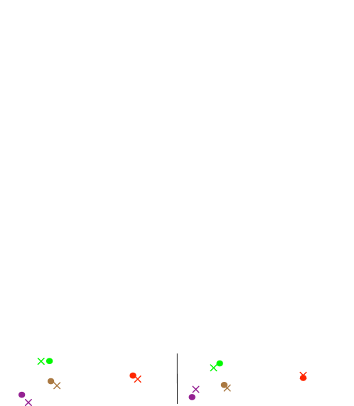
Figure 2: PCA visualization of visual and textual representations (represented in the same space) along with model’s iterations for five randomly sampled unseen classes. Circle: centroid of visual features. Cross: class label. Between even and uneven (resp. uneven and even) steps, visual centroids (resp. class labels) are moving.

4.6 Learning Grounded Word Representations with CM-GAN

In this section, we provide a post-analysis of subsection 4.5 and further validate CM-GAN by using it to visually ground language [40]. More precisely, we study the word embeddings learned in subsection 4.5, to investigate whether they capture visual information and common-sense knowledge.

The goal of grounding is to enhance textual representations using visual information. The first motivation for language grounding came from cognitive psychology studies [41, 42, 43, 44], stating that the human understanding of language is intrinsically linked to our perceptual and sensory-motor experience. It was further consolidated by quantitative-based findings such as the Human Reporting Bias [45, 46]: the frequency at which objects, relations, or events occur in natural language are significantly different from their real-world frequency — in other terms, what is obvious (visual commonsense) is rarely stated explicitly in text, since it is supposed to be known by the human reader. Following these considerations, AI researchers began to point out the lack of grounding [47] of Distributional Semantic Models such as Word2Vec [15], where the meaning of words only depends on textual co-occurrence patterns.

Unlike previous grounding models, that leverage direct correspondence between words and images , CM-GAN also exploits unsupervised information: it is thus interesting to determine whether this can enhance our word representations. Based on our CM-GAN model trained on ImageNet (subsection 4.5), we learn grounded word representations using information from seen and unseen classes. [48] has shown that a word representation $X$ given by Word2Vec (purely textual as it is learned using Word2Vec on textual corpus only) and its projection in a visual space (which is said to be grounded since visual information has been incorporated) have complementary information, that can be exploited by concatenating them. Thus, we also evaluate various concatenation combinations between $X$ and its grounded projections.

Evaluations are reported in Table 6 for standard word embeddings benchmarks [49]. First, we consider semantic relatedness benchmarks, such as WordSim353 [50], MEN [51], SimLex-999 [52], SemSim and VisSim [53], which give human judgements of similarity (e.g., between $0$ and $10$) for a series of word pairs. For each benchmark, the reported result is the Spearman correlation computed between (i) human similarity scores and (ii) the cosine similarities between word vectors. Second, we report results for the concreteness prediction task on the USF dataset [54], which gives concreteness scores for 3260 English words. A SVM model is trained to predict these scores from the word vector. The reported result is the accuracy on a test set.

We use the original Word2Vec vectors (dimension $d=300$) as $T_{0}$ representations. We note $V_{\text{sup}}(X)$ (resp. $V_{\text{trans}}(X)$) the cross-modal projection of $X$ learned using a supervised (resp. transductive) step. We observe that grounded vectors tend to outperform $X$ on all benchmarks except Concreteness, and that the information present in $X$ and the grounded vectors is complementary, as $X\oplus V_{\text{trans}}(X)$ (resp. $X\oplus V_{\text{sup}}(X)$) outperforms both $X$ and $V_{\text{trans}}(X)$ (resp. $V_{\text{sup}}(X)$). Interestingly, we notice that $X\oplus V_{\text{trans}}(X)$ gives the highest performance, thus showing the efficiency of exploiting unsupervised visual information using CM-GAN.

Model	MEN	SemSim	SimLex	VisSim	WordSim	Conc.	Avg.
$X$	68	60	33	49	62	63	55.8
$V_{\text{sup}}(X)$	69	66	34	57	59	59	57.3
$X\oplus V_{\text{sup}}(X)$	70	69	36	58	59	58	58.3
$V_{\text{trans}}(X)$	70	62	35	51	62	62	57
$X\oplus V_{\text{trans}}(X)$	72	69	37	55	58	64	59.2
$V_{\text{sup}}(X)\oplus V_{\text{trans}}(X)$	70	69	36	58	59	58	58.3

Table 6: Grounded vectors evaluation. Concatenated vectors were projected with PCA so that all vectors have the same dimension.

4.7 Zero-Shot Sentence-to-Image Matching

	Text to Image				Image to Text
Model	MFR	$FH_{1}$	$FH_{5}$	$FH_{10}$	MFR	$FH_{1}$	$FH_{5}$	$FH_{10}$
Rand.	50	0.1	0.5	1	50	0.1	0.5	1
CONSE	20.3	3.3	13.9	23.5	14.1	2.8	12.3	20.2
$\mathcal{L}_{gan}$	21	4.2	15.7	25.2	14.1	3.1	15.1	23.7
$\mathcal{L}_{c}$	18.3	4.7	14.3	24	11.3	3.7	16.6	27.3
$\mathcal{L}_{cgan}$	15.7	5.7	17.2	27.7	11.1	4.1	15.5	27.7
$\mathcal{L}_{sup}$	7.3	8.3	26.3	39.8	4.5	7.1	28.1	44.7

Table 7: Cross-modal retrieval results on MS COCO.

In this section, we demonstrate that CycleGan can align the visual and textual modalities without any supervision. We also show that CM-GAN can be applied to other settings than ImageNet: (i) replacing words by sentences, and (ii) with as many classes as training examples (590K sentences).

We evaluate several scenarios of our model on the standard cross-modal retrieval task: given a sentence, retrieving the closest image (Text to Image) and vice versa (Image to Text), in Table 7. We observe that (1) the initialization (CONSE) already shows substantial improvement compared to the Random baseline, (2) models based on CycleGAN improve performances compared to the CONSE model, due to the beneficial action of the CycleGAN loss, (3) CM-GAN has much lower performance than the Supervised baseline (where $\mathcal{L}_{sup}$ is learned), which is intuitively expected.

5 Conclusion and Future Works

In this paper, we propose the CM-GAN model for T-ZSL. We demonstrate that: (1) CM-GAN is successful on the ImageNet T-ZSL task, with state-of-the-art results, (2) visual and textual modalities can be somewhat aligned without supervision on a zero-shot sentence-to-image task on MS COCO, (3) textual representations can be enhanced using CM-GAN.

We conclude that there is meaningful information to be exploited in the similarities between textual and visual distributions, even in cases where there is no direct text/vision supervision. We showed it for three multimodal tasks: Transductive Zero-Shot Learning, Zero-Shot Image-to-Sentence Matching and Visual Grounding of Language.

We now present research perspectives.

First, to improve performances on the Zero-Shot Sentence-to-Image Matching task, an interesting perspective would be to encode sentences and images using recent improvements on Multimodal Language Models, such as LXMERT [55] or VisualBERT [56]. Indeed, these models enable to produce cross-modal representations that could be integrated within our Cross-Modal model.

Another interesting perspective would be to consider ZSL learning with noisy text descriptions, instead of class labels. Even though ZSL is mostly focused on classifying images with class labels (e.g, Abyssinian cat, dog, traffic light), some works [57, 58] have proposed, instead, to consider noisy text descriptions e.g, The Parakeet Auklet is a small (23cm) auk with a short orange bill that is upturned … We could apply our CrossModal CycleGAN model to this task: to do so, we would need to select useful information in the text (visual words like small or orange for example) and represent the text as a weighted linear combination of these salient words. We could even consider a fully unsupervised configuration (as done in the zero-shot text-to-image matching task) in which we do not use a direct supervision between images and textual descriptions.

References

- [1] J. Deng, W. Dong, R. Socher, L.-J. Li, K. Li, L. Fei-Fei, ImageNet: A Large-Scale Hierarchical Image Database, in: CVPR, 2009.
- [2] E. Real, A. Aggarwal, Y. Huang, Q. V. Le, Regularized evolution for image classifier architecture search, in: AAAI, 2019. doi:10.1609/aaai.v33i01.33014780.
- [3] A. Frome, G. S. Corrado, J. Shlens, S. Bengio, J. Dean, M. Ranzato, T. Mikolov, Devise: A deep visual-semantic embedding model, in: NeurIPS, 2013.
- [4] M. Palatucci, D. Pomerleau, G. E. Hinton, T. M. Mitchell, Zero-shot learning with semantic output codes, in: NeurIPS, 2009.
- [5] D. Parikh, K. Grauman, Relative attributes, in: ICCV, 2011. doi:10.1109/ICCV.2011.6126281.
- [6] Y. Fu, T. M. Hospedales, T. Xiang, S. Gong, Transductive multi-view zero-shot learning, IEEE Trans. Pattern Anal. Mach. Intell. 37 (11). doi:10.1109/TPAMI.2015.2408354.
- [7] M. Ye, Y. Guo, Zero-shot classification with discriminative semantic representation learning, in: CVPR 2017, 2017. doi:10.1109/CVPR.2017.542.
- [8] Z. Wan, D. Chen, Y. Li, X. Yan, J. Zhang, Y. Yu, J. Liao, Transductive zero-shot learning with visual structure constraint, NeurIPS.
- [9] A. Zhao, M. Ding, J. Guan, Z. Lu, T. Xiang, J. Wen, Domain-invariant projection learning for zero-shot recognition, in: NeurIPS, 2018.
- [10] J. Zhu, T. Park, P. Isola, A. A. Efros, Unpaired image-to-image translation using cycle-consistent adversarial networks, in: ICCV, 2017. doi:10.1109/ICCV.2017.244.
- [11] G. Lample, A. Conneau, M. Ranzato, L. Denoyer, H. Jégou, Word translation without parallel data, in: ICLR, 2018.
- [12] M. Norouzi, T.Mikolov, S. Bengio, Y. Singer, J. Shlens, A. Frome, G. Corrado, J. Dean, Zero-shot learning by convex combination of semantic embeddings, ICLRarXiv:1312.5650.
- [13] V. Khare, D. Mahajan, H. Bharadhwaj, V. K. Verma, P. Rai, A generative framework for zero-shot learning with adversarial domain adaptation, CoRR abs/1906.03038. arXiv:1906.03038.
- [14] H. Huang, C. Wang, P. S. Yu, C. Wang, Generative dual adversarial network for generalized zero-shot learning, in: IEEE Conference on Computer Vision and Pattern Recognition, CVPR 2019, Long Beach, CA, USA, June 16-20, 2019, 2019, pp. 801–810. doi:10.1109/CVPR.2019.00089.
- [15] T. Mikolov, I. Sutskever, K. Chen, G. S. Corrado, J. Dean, Distributed representations of words and phrases and their compositionality, in: NeurIPS, 2013.
- [16] S. Changpinyo, W. Chao, B. Gong, F. Sha, Synthesized classifiers for zero-shot learning, in: CVPR, 2016. doi:10.1109/CVPR.2016.575.
- [17] S. Changpinyo, W. Chao, F. Sha, Predicting visual exemplars of unseen classes for zero-shot learning, in: ICCV, 2017. doi:10.1109/ICCV.2017.376.
- [18] M. Kampffmeyer, Y. Chen, X. Liang, H. Wang, Y. Zhang, E. P. Xing, Rethinking knowledge graph propagation for zero-shot learning (2019) CVPRdoi:10.1109/CVPR.2019.01175.
- [19] Y. Fujiwara, G. Irie, Efficient label propagation, in: ICML, 2014.
- [20] F. Jurie, M. Bucher, S. Herbin, Generating visual representations for zero-shot classification, in: ICCV, 2017. doi:10.1109/ICCVW.2017.308.
- [21] J. Ni, S. Zhang, H. Xie, Dual adversarial semantics-consistent network for generalized zero-shot learning, in: Advances in Neural Information Processing Systems 32: Annual Conference on Neural Information Processing Systems 2019, NeurIPS 2019, 8-14 December 2019, Vancouver, BC, Canada, 2019, pp. 6143–6154.
- [22] V. K. Verma, P. Rai, A simple exponential family framework for zero-shot learning, in: ECML PKDD 2017, 2017. doi:10.1007/978-3-319-71246-8\_48.
- [23] A. Mishra, M. S. K. Reddy, A. Mittal, H. A. Murthy, A generative model for zero shot learning using conditional variational autoencoders, in: CVPR Workshops, 2018. doi:10.1109/CVPRW.2018.00294.
- [24] Y. Xian, S. Sharma, B. Schiele, Z. Akata, F-VAEGAN-D2: A feature generating framework for any-shot learning, in: IEEE Conference on Computer Vision and Pattern Recognition, CVPR 2019, Long Beach, CA, USA, June 16-20, 2019, 2019, pp. 10275–10284. doi:10.1109/CVPR.2019.01052.
- [25] J. Zhao, J. Zhang, Z. Li, J. Hwang, Y. Gao, Z. Fang, X. Jiang, B. Huang, Dd-cyclegan: Unpaired image dehazing via double-discriminator cycle-consistent generative adversarial network, EAAIdoi:10.1016/j.engappai.2019.04.003.
- [26] Y. Chung, W. Weng, S. Tong, J. R. Glass, Unsupervised cross-modal alignment of speech and text embedding spaces, in: NeurIPS, 2018.
- [27] E. Bruni, N. Tran, M. Baroni, Multimodal distributional semantics, J. Artif. Intell. Res.doi:10.1613/jair.4135.
- [28] K. He, X. Zhang, S. Ren, J. Sun, Deep residual learning for image recognition, in: CVPR, 2016. doi:10.1109/CVPR.2016.90.
- [29] P. Bordes, E. Zablocki, L. Soulier, B. Piwowarski, P. Gallinari, Incorporating visual semantics into sentence representations within a grounded space, in: EMNLP-IJCNLP, 2019. doi:10.18653/v1/D19-1064.
- [30] K. Q. Weinberger, L. K. Saul, Distance metric learning for large margin nearest neighbor classification, J. Mach. Learn. Res. 10 (2009) 207–244.
- [31] R. Hadsell, S. Chopra, Y. LeCun, Dimensionality reduction by learning an invariant mapping, in: CVPR, 2006, pp. 1735–1742. doi:10.1109/CVPR.2006.100.
- [32] I. J. Goodfellow, J. Pouget-Abadie, M. Mirza, B. Xu, D. Warde-Farley, S. Ozair, A. C. Courville, Y. Bengio, Generative adversarial nets, in: NeurIPS, 2014.
- [33] T. Lin, M. Maire, S. J. Belongie, J. Hays, P. Perona, D. Ramanan, P. Dollár, C. L. Zitnick, Microsoft COCO: common objects in context, in: ECCV, 2014. doi:10.1007/978-3-319-10602-1\_48.
- [34] E. Zablocki, P. Bordes, L. Soulier, B. Piwowarski, P. Gallinari, Context-aware zero-shot learning for object recognition, in: ICML, 2019.
- [35] W. Wang, Y. Pu, V. K. Verma, K. Fan, Y. Zhang, C. Chen, P. Rai, L. Carin, Zero-shot learning via class-conditioned deep generative models, in: AAAI, 2018.
- [36] V. K. Verma, G. Arora, A. Mishra, P. Rai, Generalized zero-shot learning via synthesized examples, in: CVPR, 2018. doi:10.1109/CVPR.2018.00450.
- [37] C. Szegedy, V. Vanhoucke, S. Ioffe, J. Shlens, Z. Wojna, Rethinking the inception architecture for computer vision, in: CVPR, 2016. doi:10.1109/CVPR.2016.308.
- [38] A. Krizhevsky, I. Sutskever, G. E. Hinton, Imagenet classification with deep convolutional neural networks, Commun. ACMdoi:10.1145/3065386.
- [39] B. S. Y. Xian, C. H. Lampert, Z. Akata, Zero-shot learning - A comprehensive evaluation of the good, the bad and the ugly, IEEEdoi:10.1109/TPAMI.2018.2857768.
- [40] A. Lazaridou, N. T. Pham, M. Baroni, Combining language and vision with a multimodal skip-gram model, in: NAACL, 2015. doi:10.3115/v1/n15-1016.
- [41] M. De Vega, A. Glenberg, A. Graesser, Symbols and embodiment: Debates on meaning and cognition, Oxford University Press, 2012. doi:10.1093/acprof:oso/9780199217274.001.0001.
- [42] F. Pulvermuller, Brain mechanisms linking language and action, Nature reviews. Neuroscience 6. doi:10.1038/nrn1706.
- [43] T. Hansen, M. Olkkonen, S. Walter, K. Gegenfurtner, Memory modulates color appearance, Nature neuroscience 9. doi:10.1038/nn1794.
- [44] M. Kaschak, R. Zwaan, M. Aveyard, R. Yaxley, Perception of auditory motion affects language processing, Cognitive science 30. doi:10.1207/s15516709cog0000_54.
- [45] J. Gordon, B. Van Durme, Reporting bias and knowledge acquisition, in: Proceedings of the 2013 workshop on Automated knowledge base construction - AKBC ’13, 2013. doi:10.1145/2509558.2509563.
- [46] I. Misra, C. L. Zitnick, M. Mitchell, R. B. Girshick, Seeing through the human reporting bias: Visual classifiers from noisy human-centric labels, in: CVPR 2016, 2016. doi:10.1109/CVPR.2016.320.
- [47] M. Baroni, Grounding distributional semantics in the visual world, Language and Linguistics Compass 10 (1). doi:10.1111/lnc3.12170.
- [48] G. Collell, T. Zhang, M. Moens, Imagined visual representations as multimodal embeddings, in: AAAI, 2017.
- [49] É. Zablocki, B. Piwowarski, L. Soulier, P. Gallinari, Learning Multi-Modal Word Representation Grounded in Visual Context, in: AAAI, 2018.
- [50] L. Finkelstein, E. Gabrilovich, Y. Matias, E. Rivlin, Z. Solan, G. Wolfman, E. Ruppin, Placing search in context: the concept revisited, ACMdoi:10.1145/503104.503110.
- [51] E. Bruni, N. Tran, M. Baroni, Multimodal distributional semantics, J. Artif. Intell. Res. 49. doi:10.1613/jair.4135.
- [52] F. Hill, R. Reichart, A. Korhonen, Simlex-999: Evaluating semantic models with (genuine) similarity estimation, Computational Linguistics 41 (4). doi:10.1162/COLI\_a\_00237.
- [53] C. Silberer, M. Lapata, Learning grounded meaning representations with autoencoders, in: ACL, 2014.
- [54] D. L. Nelson, C. L. McEvoy, T. A. Schreiber, The university of south florida free association, rhyme, and word fragment norms, Behavior Research Methods, Instruments, & Computers 36 (3). doi:10.3758/BF03195588.
- [55] H. Tan, M. Bansal, LXMERT: learning cross-modality encoder representations from transformers, in: Proceedings of the 2019 Conference on Empirical Methods in Natural Language Processing and the 9th International Joint Conference on Natural Language Processing, EMNLP-IJCNLP 2019, Hong Kong, China, November 3-7, 2019, 2019, pp. 5099–5110. doi:10.18653/v1/D19-1514.
- [56] L. H. Li, M. Yatskar, D. Yin, C. Hsieh, K. Chang, Visualbert: A simple and performant baseline for vision and language, CoRR abs/1908.03557. arXiv:1908.03557.
- [57] M. Elhoseiny, Y. Zhu, H. Zhang, A. M. Elgammal, Link the head to the ”beak”: Zero shot learning from noisy text description at part precision, in: 2017 IEEE Conference on Computer Vision and Pattern Recognition, CVPR 2017, Honolulu, HI, USA, July 21-26, 2017, 2017, pp. 6288–6297. doi:10.1109/CVPR.2017.666.
- [58] Y. Zhu, M. Elhoseiny, B. Liu, X. Peng, A. Elgammal, A generative adversarial approach for zero-shot learning from noisy texts, in: 2018 IEEE Conference on Computer Vision and Pattern Recognition, CVPR 2018, Salt Lake City, UT, USA, June 18-22, 2018, 2018, pp. 1004–1013. doi:10.1109/CVPR.2018.00111.