Unified Multi-Modal Landmark Tracking
for Tightly Coupled Lidar-Visual-Inertial Odometry

Abstract

We present an efficient multi-sensor odometry system for mobile platforms that jointly optimizes visual, lidar, and inertial information within a single integrated factor graph. This runs in real-time at full framerate using fixed lag smoothing. To perform such tight integration, a new method to extract 3D line and planar primitives from lidar point clouds is presented. This approach overcomes the suboptimality of typical frame-to-frame tracking methods by treating the primitives as landmarks and tracking them over multiple scans. True integration of lidar features with standard visual features and IMU is made possible using a subtle passive synchronization of lidar and camera frames. The lightweight formulation of the 3D features allows for real-time execution on a single CPU. Our proposed system has been tested on a variety of platforms and scenarios, including underground exploration with a legged robot and outdoor scanning with a dynamically moving handheld device, for a total duration of $96\text{\,}\mathrm{min}\text{/}$ and $2.4\text{\,}\mathrm{km}\text{/}$ traveled distance. In these test sequences, using only one exteroceptive sensor leads to failure due to either underconstrained geometry (affecting lidar) or textureless areas caused by aggressive lighting changes (affecting vision). In these conditions, our factor graph naturally uses the best information available from each sensor modality without any hard switches.

I Introduction

Multi-modal sensor fusion is a key capability required for successful deployment of autonomous navigation systems in real-world scenarios. The spectrum of possible applications is wide, ranging from autonomous underground exploration to outdoor dynamic mapping (see Fig. 1).

Recent advances in lidar hardware have fostered research into lidar-inertial fusion [1, 2, 3, 4]. The wide field-of-view, density, range, and accuracy of lidar sensors makes them suitable for navigation, localization, and mapping tasks.

However, in environments with degenerate geometries, such as long tunnels or wide open spaces, lidar-only approaches can fail. Since the IMU integration alone cannot provide reliable pose estimates for more than a few seconds, the system failure is often unrecoverable. To cope with these situations, fusion with additional sensors, in particular cameras, is also required. While visual-inertial-lidar fusion has already been achieved in the past via loosely coupled methods [5], tightly coupled methods such as incremental smoothing are more desirable because of their superior robustness.

In the domain of smoothing methods, research on Visual-Inertial Navigation Systems (VINS) is now mature and lidar-inertial systems are becoming increasingly popular. However, the tight fusion of all three sensor modalities at once is still an open research problem.

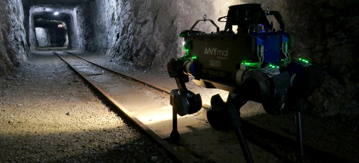
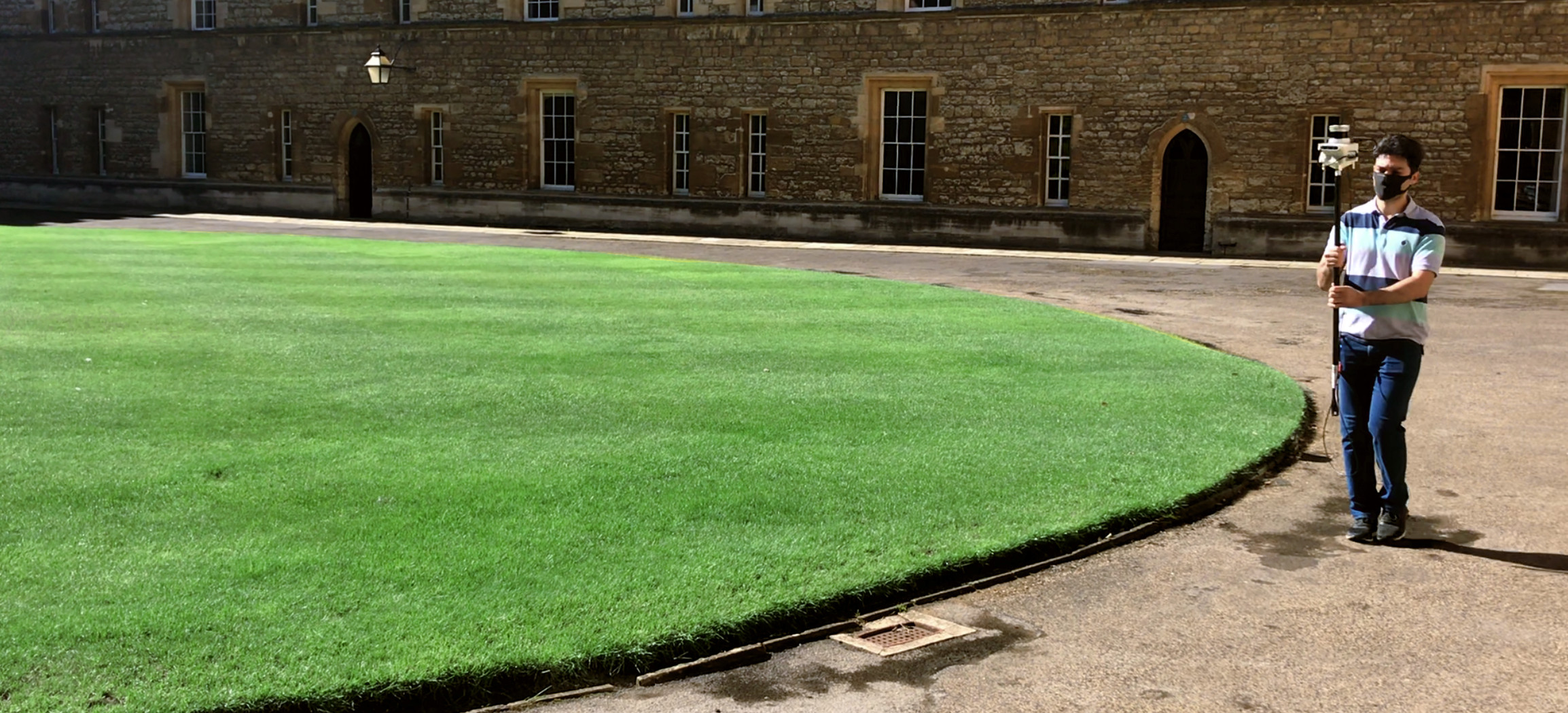
Figure 1: We tested our multi-sensor odometry algorithm with data from the ANYmal quadruped robot [6] in the DARPA SubT Challenge (top, courtesy RSL/ETH Zurich) and a handheld mapping device in New College, Oxford [7] (bottom). Video: https://youtu.be/MjXYAHurWe8

I-A Motivation

The two major challenges associated with the fusion of IMU, lidar and camera sensing are: 1) achieving real-time performance given the limited computational budget of mobile platforms and 2) the appropriate synchronization of three signals running at different frequencies and methods of acquisition.

Prior works have addressed these two problems by adopting loosely coupled approaches [5, 8, 9] or by running two separate systems (one for lidar-inertial and the other for visual-inertial odometry) [10].

Instead, we are motivated to tackle these problems by: 1) extracting and tracking sparse lightweight primitives and 2) developing a coherent factor graph which leverages IMU pre-integration to transform dynamically dewarped point clouds to the timestamp of nearby camera frames. The former avoids matching entire point clouds (e.g. ICP) or tracking hundreds of feature points (as in LOAM [1]). The latter makes real-time smoothing of all the sensors possible.

I-B Contribution

The main contributions of this work are the following:

• A novel factor graph formulation that tightly fuses vision, lidar and IMU measurements within a single consistent optimization process;

• An efficient method for extracting lidar features, which are then optimized as landmarks. Both lidar and visual features share a unified representation, as the landmarks are all treated as $n$-dimensional parametric manifolds (i.e., points, lines and planes). This compact representation allows us to process all the lidar scans at nominal framerate;

• Extensive experimental evaluation across a range of scenarios demonstrating superior robustness when compared to more typical approaches which struggle when individual sensor modalities fail.

Our work builds upon the VILENS estimation system introduced in our previous works [11, 12] by adding lidar feature tracking and lidar-aided visual tracking. The combination of camera and lidar enables the use on portable devices even when moving aggressively, as it naturally handles degeneracy in the scene (either due to a lack of lidar or visual features).

II Related Work

Prior works on multi-modal sensor fusion use combinations of lidar, camera and IMU sensing and can be characterised as either loosely or tightly coupled, as summarized in Table I. Loosely coupled systems process the measurements from each sensor separately and fuse them within a filter, where they are marginalized to get the current state estimate. Alternatively, tightly coupled systems jointly optimize both past and current measurements to obtain a complete trajectory estimate.

Another important distinction is between odometry systems and SLAM systems. In the latter, loop closures are performed to keep global consistency of the estimate once the same place is visited twice. Even though some of the works in the table also include a pose-graph SLAM backend, we are mainly interested in high-frequency odometry here.

Sensors	Loosely coupled systems	Tightly coupled systems
Lidar + IMU	LOAM⋆[1], LEGO-LOAM⋆[2], SLAM with point and plane†[13]	LIPS[3], LIOM[4], LIO-SAM[14]
Vision + Lidar + IMU	V-LOAM[8], Visual-Inertial- Laser SLAM[9], Multi-modal Sensor Fusion[15]‡, Pronto[5]	LIMO[16], VIL-SLAM[10], INS with Point and Plane feature[17], LIC-Fusion[18], LIC-Fusion 2.0[19]
⋆ IMU is optional, † Lidar only solution, ‡ Additional thermal camera.

TABLE I: Different multi-modal odometry estimation algorithms

II-A Loosely Coupled Lidar-Inertial Odometry

Lidar-based odometry has gained popularity thanks to the initial work of Zhang et al. [1], who proposed the LOAM algorithm. One of their key contributions is the definition of edge and planar 3D feature points which are tracked frame-to-frame. The motion between two frames is linearly interpolated using an IMU running at high-frequency. This motion prior is used in the fine matching and registration of the features to achieve high accuracy odometry. Shan et al. [2] proposed LeGO-LOAM, which further improved the real-time performance of LOAM for ground vehicles by optimizing an estimate of the ground plane.

However, these algorithms will struggle to perform robustly in structure-less environments or in degenerate scenarios [20] where constraints cannot be found due to the lidar’s limited range and resolution — such as long motorways, tunnels, and open spaces.

II-B Loosely Coupled Visual-Inertial-Lidar Odometry

In many of the recent works [8, 9, 15, 5] vision was incorporated along with lidar and IMU for odometry estimation in a loosely coupled manner to provide a complementary sensor modality to both avoid degeneracy and have a smoother estimated trajectory over lidar-inertial systems.

The authors of LOAM extended their algorithm by integrating feature tracking from a monocular camera in V-LOAM [8] along with IMU, thereby generating a visual-inertial odometry prior for lidar scan matching. However, the operation was still performed frame-to-frame and didn’t maintain global consistency. To improve consistency, a Visual-Inertial-Lidar SLAM system was introduced by Wang et al. [9] where they used a V-LOAM based approach for odometry estimation and performed a global pose graph optimization by maintaining a keyframe database. Khattak et al. [15] proposed another loosely coupled approach similar to V-LOAM, that uses a visual/thermal inertial prior for lidar scan matching. To overcome degeneracy, the authors used visual and thermal inertial odometry so as to operate in long tunnels with no lighting. In Pronto [5], the authors used visual-inertial-legged odometry as a motion prior for a lidar odometry system and integrated pose corrections from visual and lidar odometry to correct pose drift in a loosely coupled manner.

II-C Tightly Coupled Inertial-Lidar Odometry

One of the earlier methods to tightly fuse lidar and IMU was proposed in LIPS [3], a graph-based optimization framework which optimizes the 3D plane factor derived from the closest point-to-plane representation along with preintegrated IMU measurements. In a similar fashion, Ye et al. [4] proposed LIOM, a method to jointly minimize the cost derived from lidar features and pre-integrated IMU measurements. This resulted in better odometry estimates than LOAM in faster moving scenarios. Shan et al. [14] proposed LIO-SAM, which adapted the LOAM framework by introducing scan matching at a local scale instead of global scale. This allowed new keyframes to be registered to a sliding window of prior “sub-keyframes” merged into a voxel map. The system was extensively tested on a handheld device, ground, and floating vehicles, highlighting the quality of the reconstruction of the SLAM system. For long duration navigation they also used loop-closure and GPS factors for eliminating drift.

Again, due to the absence of vision, the above algorithms may struggle to perform robustly in degenerate scenarios.

II-D Tightly Coupled Visual-Inertial-Lidar Odometry

To avoid degeneracy and to make the system more robust, tight integration of multi-modal sensing capabilities (vision, lidar, and IMU) was explored in some more recent works [10, 16, 17, 18, 19]. In LIMO [16] the authors presented a bundle adjustment–based visual odometry system. They combined the depth from lidar measurements by re-projecting them to image space and associating them to the visual features which helped to maintain accurate scale. Shao et al. [10] introduced VIL-SLAM where they combined VIO along with lidar-based odometry as separate sub-systems for combining the different sensor modalities rather than doing a joint optimization.

To perform joint state optimization, many approaches [17, 18, 19] use the Multi-State Constraint Kalman Filter (MSCKF) framework [21]. Yang et al. [17] tightly integrated the plane features from an RGB-D sensor within $3.5\text{\,}\mathrm{m}\text{/}$ range and point features from vision and IMU measurements using an MSCKF. To limit the state vector size, most of the point features were treated as MSCKF features and linearly marginalized, while only a few point features enforcing point-on-plane constraints were kept in state vector as SLAM features. LIC-Fusion introduced by Zuo et al. [18] tightly combines the IMU measurements, extracted lidar edge features, as well as sparse visual features, using the MSCKF fusion framework. Whereas, in a recent follow up work, LIC-Fusion 2.0 [19], the authors introduced a sliding window based plane-feature tracking approach for efficiently processing 3D lidar point clouds.

In contrast with previous works, we jointly optimize the three aforementioned sensor modalities within a single, consistent factor graph optimization framework. To process lidar data at real-time, we directly extract and track 3D primitives such as lines and planes from the lidar point clouds, rather than performing “point-to-plane” or “point-to-line” based cost functions. This allows for natural tracking over multiple frames in a similar fashion to visual tracking, and to constrain the motion even in degenerate scenarios.

III Problem Statement

We aim to estimate the position, orientation, and linear velocity of a mobile platform (in our experiments, a legged robot or a handheld sensor payload) equipped with IMU, lidar and either a mono or stereo camera with low latency and at full sensor rate.

The relevant reference frames are specified in Fig. 2 and include the robot-fixed base frame $\mathtt{{B}}$, left camera frame $\mathtt{C}$, IMU frame $\mathtt{I}$, and lidar frame $\mathtt{L}$. We wish to estimate the position of the base frame relative to a fixed world frame $\mathtt{W}$.

Unless otherwise specified, the position $\tensor[_{\mathtt{{W}}}]{\mathbf{p}}{{}_{\mathtt{{W}}\mathtt{{B}}}}$ and orientation $\mathbf{R}_{\mathtt{{W}}\mathtt{{B}}}$ of the base (with $\tensor[_{\mathtt{{W}}}]{\mathbf{T}}{{}_{\mathtt{{W}}\mathtt{{B}}}}\in\mathrm{SE}(3)$ as the corresponding homogeneous transform) are expressed in world coordinates; velocities $\tensor[_{\mathtt{{B}}}]{\mathbf{v}}{{}_{\mathtt{{W}}\mathtt{{B}}}},\tensor[_{\mathtt{{B}}}]{\boldsymbol{\omega}}{{}_{\mathtt{{W}}\mathtt{{B}}}}$ are in the base frame, and IMU biases $\tensor[_{\mathtt{{I}}}]{\mathbf{b}}{{}^{g}},\;\tensor[_{\mathtt{{I}}}]{\mathbf{b}}{{}^{a}}$ are expressed in the IMU frame.

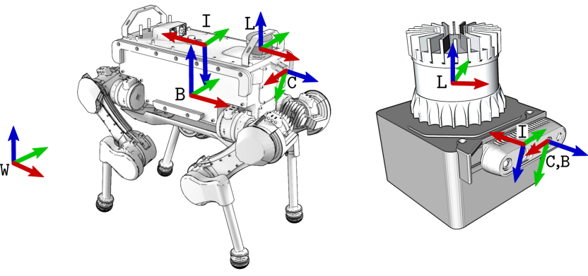
Figure 2: Reference frames conventions for the ANYmal platform and the handheld device. The world frame $\mathtt{W}$ is a fixed frame, while the base frame $\mathtt{{B}}$, camera optical frame $\mathtt{C}$, IMU frame, $\mathtt{I}$, and lidar frame $\mathtt{L}$ are attached to the moving robot’s chassis or device. For simplicity, $\mathtt{C}$ and $\mathtt{{B}}$ are coincident on the handheld device.

III-A State Definition

The mobile platform state at time $t_{i}$ is defined as follows:

$$\boldsymbol{x}_{i}\triangleq\left[\mathbf{R}_{i},\mathbf{p}_{i},\mathbf{v}_{i},\mathbf{b}^{g}_{i}\,\;\mathbf{b}^{a}_{i}\right]\in\mathrm{SO}(3)\times\mathbb{R}^{12}$$ (1)

where: $\mathbf{R}_{i}$ is the orientation, $\mathbf{p}_{i}$ is the position, $\mathbf{v}_{i}$ is the linear velocity, and the last two elements are the usual IMU gyroscope and accelerometer biases.

In addition to the states, we track the parameters of three $n$-manifolds: points, lines and planes. The point landmarks $\boldsymbol{m}_{\ell}$ are visual features, while lines $\boldsymbol{l}_{\ell}$ and planes $\boldsymbol{p}_{\ell}$ landmarks are extracted from lidar. The objective of our estimation are all states and landmarks visible up to the current time $t_{k}$:

$$\mathcal{X}_{k}\triangleq\left[\bigcup_{\forall i\in\mathsf{X}_{k}}\{\boldsymbol{x}_{i}\},\bigcup_{\forall\ell\in\mathsf{M}_{k}}\{\boldsymbol{m}_{\ell}\},\bigcup_{\forall\ell\in\mathsf{P}_{k}}\{\boldsymbol{p}_{\ell}\},\bigcup_{\forall\ell\in\mathsf{L}_{k}}\{\boldsymbol{l}_{\ell}\}\right]$$ (2)

where $\mathsf{X}_{k},\mathsf{M}_{k},\mathsf{P}_{k},\mathsf{L}_{k}$ are the lists of all states and landmarks tracked within a fixed lag smoothing window.

III-B Measurements Definition

The measurements from a mono or stereo camera ${\cal C}$, IMU ${\cal I}$, and lidar ${\cal L}$ are received at different times and frequencies. We define $\mathcal{Z}_{k}$ as the full set of measurements received within the smoothing window. Subsection V-B1 explains how the measurements are integrated within the factor graph, such that the optimization is performed at fixed frequency.

III-C Maximum-a-Posteriori Estimation

We maximize the likelihood of the measurements, ${\cal Z}_{k}$, given the history of states, ${\cal X}_{k}$:

$$\mathcal{X}^{*}_{k}=\operatorname*{arg\,max}_{\mathcal{X}_{k}}p(\mathcal{X}_{k}|\mathcal{Z}_{k})\propto p(\mathcal{X}_{0})p(\mathcal{Z}_{k}|\mathcal{X}_{k})$$ (3)

The measurements are formulated as conditionally independent and corrupted by white Gaussian noise. Therefore, Eq. (3) can be formulated as the following least squares minimization problem [22]:

$$\mathcal{X}^{*}_{k}=\operatorname*{arg\,min}_{\mathcal{X}_{k}}\sum_{i\in\mathsf{K}_{k}}\left(\|\mathbf{r}_{{\cal I}_{ij}}\|^{2}_{\Sigma_{{\cal I}_{ij}}}+\sum_{\ell\in\mathsf{P}_{i}}\|\mathbf{r}_{\boldsymbol{x}_{i},\boldsymbol{p}_{\ell}}\|^{2}_{\Sigma_{\boldsymbol{x}_{i},\boldsymbol{p}_{\ell}}}+\right.\\ \left.\sum_{\ell\in\mathsf{L}_{i}}\|\mathbf{r}_{\boldsymbol{x}_{i},\boldsymbol{l}_{\ell}}\|^{2}_{\Sigma_{\boldsymbol{x}_{i},\boldsymbol{l}_{\ell}}}+\sum_{\ell\in\mathsf{M}_{i}}\|\mathbf{r}_{\boldsymbol{x}_{i},\boldsymbol{m}_{\ell}}\|^{2}_{\Sigma_{\boldsymbol{x}_{i},\boldsymbol{m}_{\ell}}}\right)+\|\mathbf{r}_{0}\|^{2}_{\Sigma_{0}}$$ (4)

where ${\cal I}_{ij}$ are the IMU measurements between $t_{i}$ and $t_{j}$ and $\mathsf{K}_{k}$ are all keyframe indices before $t_{k}$. Each term is the residual associated to a factor type, weighted by the inverse of its covariance matrix. The residuals are: IMU, lidar plane and line features, visual landmarks, and a state prior.

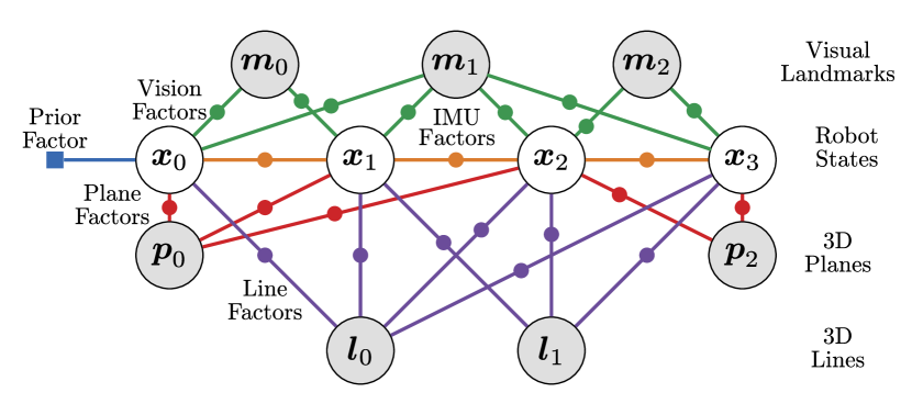
Figure 3: VILENS sliding-window factor graph structure, showing prior, visual, plane, line, and preintegrated IMU factors. Tracking landmarks over time increases the accuracy of the estimation by allowing new measurements to improve the accuracy of past states.

IV Factor Graph Formulation

We now describe the measurements, residuals, and covariances of the factors in the graph, shown in Fig. 3. For convenience, we summarize the IMU factors in Section IV-A; then, we introduce the visual-lidar landmark factors in Sections IV-B and IV-C, while Section IV-D describes our novel plane and line landmark factors.

IV-A Preintegrated IMU Factors

We follow the now standard manner of IMU measurement preintegration [23] to constrain the pose, velocity, and biases between two consecutive nodes of the graph, and provide high frequency states updates between nodes. The residual has the form:

$$\mathbf{r}_{{\cal I}_{ij}}=\left[\mathbf{r}^{\mathsf{T}}_{\Delta\mathbf{R}_{ij}},\mathbf{r}^{\mathsf{T}}_{\Delta\mathbf{v}_{ij}},\mathbf{r}^{\mathsf{T}}_{\Delta\mathbf{p}_{ij}},\mathbf{r}_{\mathbf{b}^{a}_{ij}},\mathbf{r}_{\mathbf{b}^{g}_{ij}}\right]$$ (5)

For the definition of the residuals, see [23].

IV-B Mono Landmark Factors with Lidar Depth

To take full advantage of the fusion of vision and lidar sensing modalities, we track monocular visual features but use the lidar’s overlapping field-of-view to provide depth estimates, as in [16]. To match the measurements from lidar and camera, which operate at 10 Hz and 30 Hz respectively, we use the method described in Section V-B1.

Let $\boldsymbol{m}_{\ell}\in\mathbb{R}^{3}$ be a visual landmark in Euclidean space, $\pi:\mathrm{SE}(3)\times\mathbb{R}^{3}\mapsto\mathbb{R}^{2}$ a function that projects a landmark to the image plane given a platform pose $\mathbf{T}_{i}$ (for simplicity, we omit the fixed transforms between base, lidar and camera), and $(u_{\ell},v_{\ell})\in\mathbb{R}^{2}$ a detection of $\boldsymbol{m}_{\ell}$ on the image plane (yellow dots in Fig. 4, right). We first project all the points $\tilde{\mathbf{x}}_{m}\in{\cal L}_{i}$ acquired by the lidar between time $t_{i}$ and $t_{i+1}$ onto the image plane with $\pi(\mathbf{T}_{i},\tilde{\mathbf{x}}_{m})$ (green dots in Fig. 4, right). Then, we find the projected point $\pi(\tilde{\mathbf{x}}_{\ell})$ that is closest to $(u_{\ell},v_{\ell})$ on the image plane within a neighborhood of 3 pixels. Finally, the residual is computed as:

$$\mathbf{r}_{\boldsymbol{x}_{i},\boldsymbol{m}_{\ell}}=\mathbf{T}^{-1}_{i}\boldsymbol{m}_{\ell}-\tilde{\mathbf{x}}_{\ell}$$ (6)

When we cannot associate lidar depth to a visual feature (due to the different resolution of lidar and camera sensors) or if it is unstable (i.e., when the depth changes $>$0.5\text{\,}\mathrm{m}\text{/}$$ between frames due to dynamic obstacles or noise), we revert to stereo matching, as described in the next section.

IV-C Stereo Landmark Factors

The residual at state $\boldsymbol{x}_{i}$ for landmark $\boldsymbol{m}_{\ell}$ is [12]:

$$\mathbf{r}_{\boldsymbol{x}_{i},\boldsymbol{m}_{\ell}}=\left(\begin{array}[]{c}\pi_{u}^{L}(\mathbf{T}_{i},\boldsymbol{m}_{\ell})-u^{L}_{i,\ell}\\ \pi_{u}^{R}(\mathbf{T}_{i},\boldsymbol{m}_{\ell})-u^{R}_{i,\ell}\\ \pi_{v}(\mathbf{T}_{i},\boldsymbol{m}_{\ell})-v_{i,\ell}\end{array}\right)$$ (7)

where $(u^{L},v),(u^{R},v)$ are the pixel locations of the detected landmark and $\Sigma_{\boldsymbol{m}}$ is computed from an uncertainty of $0.5$ pixels. Finally, if only a monocular camera is available, then only the first and last elements in Eq. 7 are used.

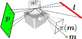
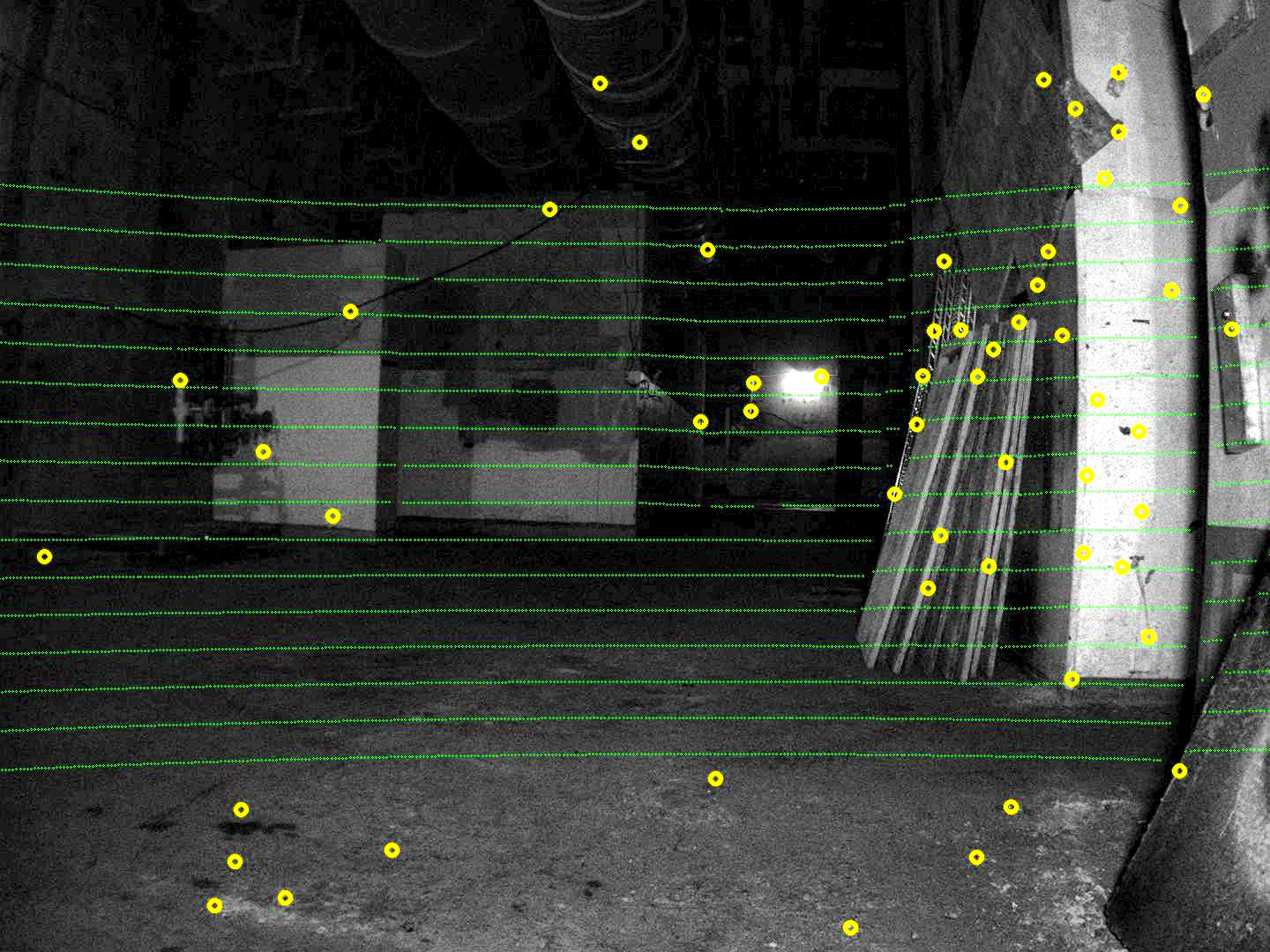
Figure 4: Left: The visual FAST features $\boldsymbol{m}$ (yellow); the lidar line $\boldsymbol{l}$: (red), and plane $\boldsymbol{p}$ primitive (green) are tracked by our method. Right: The projection of the lidar data (green) along with the visual features (yellow) into the image frame, which helps to associate depth to the visual features.

IV-D Plane Landmark Factor

We use the Hessian normal form to parametrize an infinite plane $\boldsymbol{p}$ as a unit normal $\hat{\mathbf{n}}\in\mathbb{R}^{3}$ and a scalar $d$ representing its distance from the origin:

$$\boldsymbol{p}=\left\{\langle\hat{\mathbf{n}},d\rangle\in\mathbb{R}^{4}~{}|~{}\hat{\mathbf{n}}\cdot(x,y,z)+d=0\right\}$$ (8)

Let $\otimes$ be the operator that applies a homogeneous transform $\mathbf{T}$ to all the points of a plane $\boldsymbol{p}$, and $\ominus$ the operator that defines the error between two planes $(\boldsymbol{p}_{i},\boldsymbol{p}_{j})$ as:

$$\boldsymbol{p}_{i}\ominus\boldsymbol{p}_{j}=\left(B_{p}^{\mathsf{T}}\hat{\xi},d_{i}-d_{j}\right)\in\mathbb{R}^{3}$$ (9)

where $B_{p}\in\mathbb{R}^{3\times 2}$ is a basis for the tangent space of $\hat{\mathbf{n}}_{i}$ and $\hat{\xi}$ is defined as follows [24]:

$$\hat{\xi}=-\frac{\arccos{(\hat{\mathbf{n}}_{i}\cdot\hat{\mathbf{n}}_{j})}}{1-(\hat{\mathbf{n}}_{i}\cdot\hat{\mathbf{n}}_{j})^{2}}\left(\hat{\mathbf{n}}_{j}-(\hat{\mathbf{n}}_{i}\cdot\hat{\mathbf{n}}_{j})\hat{\mathbf{n}}_{i}\right)\in\mathbb{R}^{3}$$ (10)

When a plane $\tilde{\boldsymbol{p}}_{i}$ is measured at time $t_{i}$, the corresponding residual is the difference between $\tilde{\boldsymbol{p}}$ and the estimated plane $\boldsymbol{p}_{\ell}$ transformed into the local reference frame:

$$\mathbf{r}_{x_{i},\boldsymbol{p}_{\ell}}=\left({\mathbf{T}}^{-1}_{i}\otimes\boldsymbol{p}_{\ell}\right)\ominus\tilde{\boldsymbol{p}}_{i}$$ (11)

IV-E Line Landmark Factor

Using the approach from [25], infinite straight lines can be parametrized by a rotation matrix $\mathbf{R}\in\mathrm{SO}(3)$ and two scalars $a$, $b$ $\in$ $\mathbb{R}$, such that $\hat{\mathbf{v}}=\mathbf{R}\hat{\mathbf{z}}$ is the direction of the line and $\mathbf{d}=\mathbf{R}(a\hat{\mathbf{x}}+b\hat{\mathbf{y}})$ is the closest point between the line and the origin. A line $\boldsymbol{l}$ can therefore be defined as:

$$\boldsymbol{l}=\left\{\langle\mathbf{R},(a,b)\rangle\in\mathrm{SO}(3)\times\mathbb{R}^{2}\right\}$$ (12)

Let $\boxtimes$ be the operator that applies a transform $\mathbf{T}_{ij}=(\mathbf{R}_{ij},\mathbf{p}_{ij})$ to all the points of a line $\boldsymbol{l}_{i}$ to get $\boldsymbol{l}_{j}$ such that:

$$\mathbf{R}_{j} =\mathbf{R}_{ij}\mathbf{R}_{i}$$

$$a_{j} =a_{i}-\left[\begin{smallmatrix}1&0&0\end{smallmatrix}\right]\mathbf{R}^{\mathsf{T}}_{ij}\mathbf{p}_{ij}$$

$$b_{j} =b_{i}-\left[\begin{smallmatrix}0&1&0\end{smallmatrix}\right]\mathbf{R}^{\mathsf{T}}_{ij}\mathbf{p}_{ij}$$ (13)

The error operator $\boxminus$ between two lines $\boldsymbol{l}_{i},\boldsymbol{l}_{j}$ is defined as:

$$\boldsymbol{l}_{i}\boxminus\boldsymbol{l}_{j}=\left(\left[\begin{smallmatrix}1&0\\ 0&1\\ 0&0\end{smallmatrix}\right]^{\mathsf{T}}\mathrm{Log}\left(\mathbf{R}_{i}^{\mathsf{T}}\mathbf{R}_{j}\right),a_{i}-a_{j},b_{i}-b_{j}\right)\in\mathbb{R}^{4}$$ (14)

Given Eq. 13 and Eq. 14, the residual between a measured line $\tilde{\boldsymbol{l}}_{i}$ and its prediction is defined as follows:

$$\mathbf{r}_{x_{i},\boldsymbol{l}\ell}=\left(\mathbf{T}^{-1}_{i}\boxtimes\boldsymbol{l}_{\ell}\right)\boxminus\tilde{\boldsymbol{l}}_{i}$$ (15)

We use the numerical derivatives of Eq. (11) and (15) in the optimization, using the symmetric difference method.

V Implementation

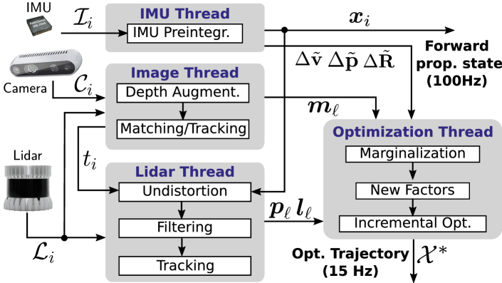
Figure 5: Overview of the VILENS system architecture. The inputs are handled in separate threads by each front-end measurement handler. The back-end produces both a high frequency forward-propagated output and a lower frequency optimized output. This parallel architecture allows for different measurement inputs depending on the platform.

The system architecture is shown in Fig. 5. Using four parallel threads for the sensor processing and optimization, the system outputs the state estimated by the factor-graph at camera keyframe frequency (typically $15\text{\,}\mathrm{Hz}\text{/}$) and the IMU forward-propagated state at IMU frequency (typically $100\text{\,}\mathrm{Hz}\text{/}$) for use in navigation/mapping and control respectively.

The factor graph is solved using a fixed lag smoothing framework based on the efficient incremental optimization solver iSAM2, using the GTSAM library [22]. For these experiments, we use a lag time of between $5$ and $10\text{\,}\mathrm{s}\text{/}$. All visual and lidar factors are added to the graph using the Dynamic Covariance Scaling (DCS) [26] robust cost function to reduce the effect of outliers.

V-A Visual Feature Tracking

We detect features using the FAST corner detector, and track them between successive frames using the KLT feature tracker with outliers rejected using RANSAC. Thanks to the parallel architecture and incremental optimization, every second frame is used as a keyframe, achieving $15\text{\,}\mathrm{Hz}\text{/}$ nominal output.

V-B Lidar Processing and Feature Tracking

A key feature of our algorithm is that we extract feature primitives from the lidar point clouds represented at the same time as a camera frame, such that the optimization can be executed for all the sensors at once. The processing pipeline consists of the following steps: point cloud undistortion and synchronization, filtering, primitive extraction and tracking, and factor creation.

V-B1 Undistortion and Synchronization

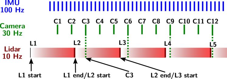
Figure 6: Example of output frequencies and synchronization between IMU, camera and lidar. IMU and camera signals are captured instantaneously, while lidar points are captured and accumulated for $0.1\text{\,}\mathrm{s}\text{/}$ before being sent as a scan. When the scan L2 is received, it is undistorted to the same time as camera frame C3 and added to the same graph node as the camera.

Fig. 6 compares the different output frequencies of our sensors. While IMU and camera samples are captured instantaneously, lidars continually capture points while their internal mirror rotates around the $z$-axis. Once a full rotation is complete, the accumulated laser returns are converted into a point cloud and a new scan starts immediately thereafter.

Since the laser returns are captured while moving, the point cloud needs to be undistorted with a motion prior and associated to a unique arbitrary timestamp – typically the start of the scan [27]. This approach would imply that camera and lidar measurements have different timestamps and thus separate graph nodes.

Instead, we choose to undistort the lidar measurement to the closest camera timestamp after the start of the scan. For example, in Fig. 6, the scan L2 is undistorted to the timestamp of keyframe C3. Given the forward propagated states from the IMU module, the motion prior is linearly extrapolated using the timestamp associated to each point of the cloud (for simplicity, we avoid Gaussian-Process interpolation [28] or state augmentation with time offsets [29]). As the cloud is now associated with C3, the lidar landmarks are connected to the same node as C3 rather than creating a new one.

This subtle detail not only guarantees that a consistent number of new nodes and factors are added to the graph optimization, but it also ensures that the optimization is performed jointly between IMU, camera and lidar inputs. This also ensures a fixed output frequency, i.e., the camera framerate or lidar framerate (when cameras are unavailable), but not a mixture of the two.

V-B2 Filtering

Once the point cloud has been undistorted, we perform the segmentation from [30] to separate the points into clusters. Small clusters (less than 5 points) are marked as outliers and discarded as they are likely to be noisy.

Then, the local curvature of each point in the pre-filtered cloud is calculated using the approach of [2]. The points with the lowest and highest curvature are assigned to the set of plane candidates ${\cal C}_{P}$ and line candidates ${\cal C}_{L}$, respectively.

The segmentation and curvature-based filtering typically reduce the number of points in the point cloud by 90%, providing significant computational savings in the subsequent plane and line processing.

V-B3 Plane and Line Extraction and Tracking

Over time, we track planes and lines in the respective candidate sets ${\cal C}_{P}$ and ${\cal C}_{L}$. This is done in a manner analogous to local visual feature tracking methods, where features are tracked within a local vicinity of their predicted location.

First, we take the tracked planes and lines from the previous scan, $\boldsymbol{p}_{i-1}$ and $\boldsymbol{l}_{i-1}$, and use the IMU forward propagation to predict their location in the current scan, $\hat{\boldsymbol{p}}_{i}$ and $\hat{\boldsymbol{l}}_{i}$. Then to assist local tracking, we segment ${\cal C}_{P}$ and ${\cal C}_{L}$ around the predicted feature locations using a maximum point-to-model distance. Afterwards, we perform Euclidean clustering (and normal filtering for plane features) to remove outliers. Then, we fit the model to the segmented point cloud using a PROSAC [31] robust fitting algorithm.

Finally, we check that the predicted and detected landmarks are sufficiently similar. Two planes, $\boldsymbol{p}_{i}$ and $\boldsymbol{p}_{j}$, are considered a match when difference between their normals and the distance from the origin are smaller than a threshold:

$$\delta_{n}= \left\|\arccos(\hat{\mathbf{n}}_{i}\cdot\hat{\mathbf{n}}_{j})\right\| <\alpha_{p}$$ (16)

$$\delta_{d}= \left\|\hat{\mathbf{n}}_{i}d_{i}-\hat{\mathbf{n}}_{j}d_{j}\right\| <\beta_{p}$$ (17)

Two lines $\boldsymbol{l}_{i}$ and $\boldsymbol{l}_{j}$ are considered a match if their directions and their center distances are smaller than a threshold:

$$\delta_{n}= \left\|\arccos(\hat{\mathbf{v}}_{i}\cdot\hat{\mathbf{v}}_{j})\right\| <\alpha_{l}$$ (18)

$$\delta_{d}= \left\|(\mathbf{d}_{i}-\mathbf{d}_{j})-\left((\mathbf{d}_{i}-\mathbf{d}_{j})\cdot\hat{\mathbf{v}}_{i}\right)\hat{\mathbf{v}}_{i}\right\| <\beta_{l}$$ (19)

In our case $\alpha_{p}=\alpha_{l}=0.35~{}\textnormal{rad},~{}\beta_{p}=\beta_{l}=0.5~{}\textnormal{m}$.

Once a feature has been tracked, the feature’s inliers are removed from the corresponding candidate set, and the process is repeated for the remaining landmarks.

After tracking is complete, we detect new landmarks in the remaining candidate clouds. The point cloud is first divided using Euclidean clustering for lines, and normal-based region growing for planes. We then detect new landmarks in each cluster using the same method as landmark tracking.

Point cloud features are only included in the optimization after they have been tracked for a minimum number of consecutive scans. Note that the oldest features are tracked first, to ensure the longest possible feature tracks.

V-C Zero Velocity Update Factors

To limit drift and factor graph growth when the platform is stationary, we add zero velocity constraints to the graph when updates from two out of three modalities (camera, lidar, IMU) report no motion.

VI Experimental Results

We evaluated our algorithm on a variety of indoor and outdoor environments in two contrasting datasets: the Newer College Dataset [7] and the DARPA SubT Challenge (Urban). An overview of these environments is shown in Fig. 7.

VI-A Datasets

The Newer College dataset (NC) [7] was collected using a portable device equipped with a Ouster OS1-64 Gen1 lidar sensor, a RealSense D435i stereo IR camera, and an Intel NUC PC. The cellphone-grade IMU embedded in the lidar was used for inertial measurements. The device was carried by a person walking outdoor surrounded by buildings, large open spaces, and dense foliage. The dataset includes challenging sequences where the device was shaken aggressively to test the limits of tracking.

The SubT dataset (ST) consists of two of the most significant runs of the SubT competition (Alpha-2 and Beta-2) collected on two copies of the ANYmal B300 quadruped robot [6] equipped with a Flir BFS-U3-16S2C-CS monocular camera and a industrial-grade Xsens MTi-100 IMU, which were hardware synchronized by a dedicated board [32]. A Velodyne VLP-16 was also available but was synchronized via software. The robots navigated the underground interiors of an unfinished nuclear reactor. This dataset is challenging due to the presence of long straight corridors and extremely dark environments. Note that the leg kinematics from the robot was not used in this work.

The specific experiments are named as follows:

• NC-1: Walking around an open college environment ($1134\text{\,}\mathrm{m}\text{/}$, $17\text{\,}\mathrm{min}\text{/}$).

• NC-2: Walking with highly dynamic motion in the presence of strong illumination changes ($480\text{\,}\mathrm{m}\text{/}$, $6\text{\,}\mathrm{min}\text{/}$).

• NC-3: Shaking the sensor rig at very high angular velocities, up to $3.37\text{\,}\mathrm{rad}\mathrm{/}\mathrm{s}$ ($91\text{\,}\mathrm{m}\text{/}$, $2\text{\,}\mathrm{min}\text{/}$).

• ST-A: Anymal quadruped robot trotting in dark underground reactor facility ($167\text{\,}\mathrm{m}\text{/}$, $11\text{\,}\mathrm{min}\text{/}$).

• ST-B: A different Anymal robot in a part of the reactor containing a long straight corridor ($490\text{\,}\mathrm{m}\text{/}$, $60\text{\,}\mathrm{min}\text{/}$).

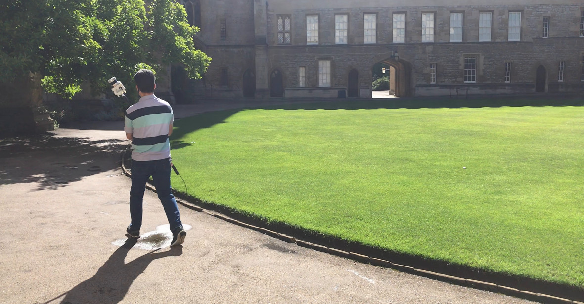
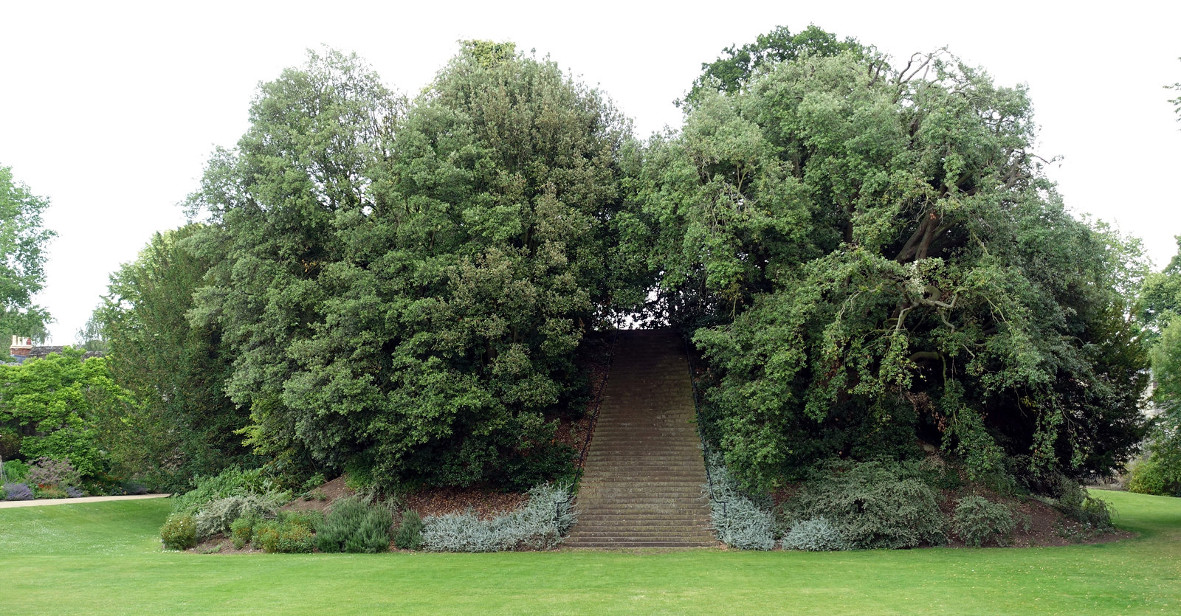
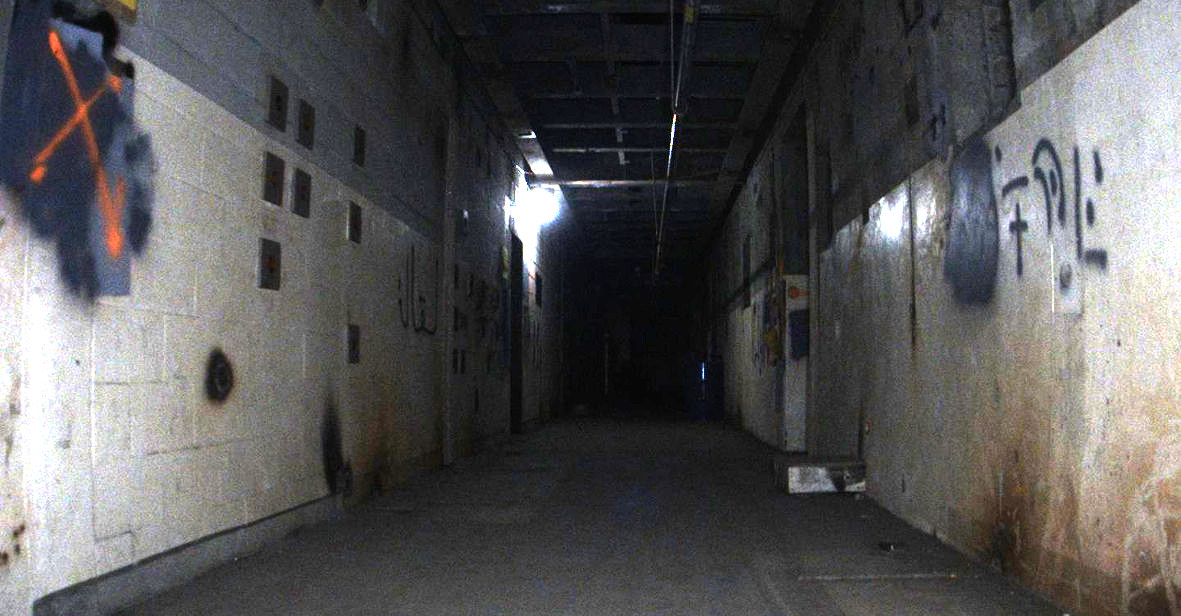
Figure 7: Top: The Newer College dataset [7] – challenges include large open spaces, dense foliage without clear structure, and large illumination changes from sunlight to shadow. Bottom: The DARPA SubT dataset – challenges include long straight corridors and low light conditions (the bottom images were manually enhanced to show the content).

To generate ground truth, ICP was used to align the current lidar scan to detailed prior maps, collected using a commercial laser mapping system. For an in-depth discussion on ground truth generation the reader is referred to [7].

Relative Pose Error (RPE) – Translation [$\mathrm{m}\text{/}$] / Rotation [$\mathrm{\SIUnitSymbolDegree}\text{/}$]
SubT Challenge Urban (ANYmal B300)
Data	VILENS-LI	VILENS-LVI	LOAM
ST-A	0.28 / 2.65	0.14 / 1.04	0.20 / 1.32
ST-B	0.20 / 1.75	0.12 / 0.79	0.22 / 0.99
Newer College (Handheld Device [7])
Data	VILENS-LI	VILENS-LVI	LeGO-LOAM
NC-1	0.50 / 3.23	0.39 / 2.45	0.34 / 3.45
NC-2	0.78 / 2.38	0.43 / 1.85	12.32 / 55.00
NC-3	0.18 / 3.12	0.20 / 3.61	1.85 / 23.67

TABLE II: Experimental Results

VI-B Results

Table II summarizes the mean Relative Pose Error (RPE) over a distance of $10\text{\,}\rm{m}$ for the following algorithms:

• VILENS-LI: VILENS with IMU and lidar only;

• VILENS-LVI: VILENS with IMU, visual (with lidar depth), and lidar features;

• LOAM: The output of the LOAM [1] mapping module used during the SubT competition.

• LeGO-LOAM: The output of the LeGO-LOAM [2] mapping module.

It should be noted that no loop closures have been performed, and in contrast to both LOAM and LeGO-LOAM methods we do not perform any mapping.

For the SubT datasets, VILENS-LVI outperforms LOAM in translation / rotation by an average of 38% / 21% and VILENS-LI by 46% / 21%. An example of the global performance is shown in Fig. 8, which depicts both the estimated and ground truth trajectories on the ST-A dataset. VILENS-LVI is able to achieve very slow drift rates, even without a mapping system or loop closures.

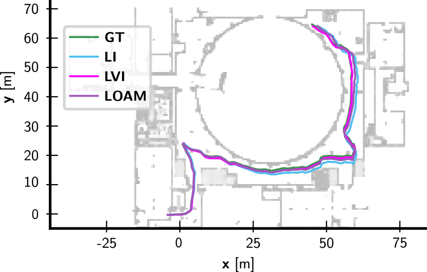
Figure 8: Aerial view and elevation over time on the ST-A dataset, showing the estimated trajectory with Lidar-Inertial (blue), Lidar-Visual-Inertial (magenta), and LOAM [1] against the ground truth (green). Note that there are no loop-closures present in this system.

For the least dynamic NC dataset, NC-1, VILENS-LVI achieves comparable performance to LeGO-LOAM. However, For the more dynamic datasets (up to $3.37\text{\,}\mathrm{rad}\mathrm{/}\mathrm{s}$), NC-2 and NC-3, the VILENS methods significantly outperform LeGO-LOAM. Key to this performance is the undistortion of the lidar cloud to the camera timestamp, allowing accurate visual feature depth-from-lidar, while minimizing computation.

Overall, the best performing algorithm was VILENS-LVI, showing how the tight integration of visual and lidar features allows us to avoid failure modes that may be present in lidar-inertial only methods.

VI-C Multi-Sensor Fusion

A key benefit arising from the tight fusion of complementary sensor modalities is a natural robustness to sensor degradation. While a significant proportion of the datasets presented favorable conditions for both lidar and visual feature tracking, there were a number of scenarios where the tight fusion enabled increased robustness to failure modes of individual sensors.

Fig. 9 shows an example from the NC-2 where the camera auto-exposure feature took $\sim 3\text{\,}\mathrm{s}\text{/}$ to adjust when moving out of bright sunlight into shade. During this time the number of visual features drops from around 30 to less than 5 (all clustered in a corner of the image). This would cause instability in the estimator. By tightly fusing the lidar, we are able to use the small number of visual features and the lidar features, without causing any degradation in performance. This is in contrast to methods such as [5, 15] where the use of separate visual-inertial and lidar-inertial subsystems mean that degenerate situations must be explicitly handled.

Similarly, in cases where the lidar landmarks are not sufficient to fully constrain the estimate (or are close to degenerate), the tight fusion of visual features allow the optimisation to take advantage of the lidar constraints while avoiding problems with degeneracy.

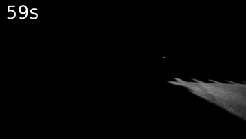
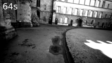
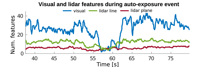
Figure 9: Top: The Newer College (NC-2) contains sections with dramatic exposure change from underexposure (left) to more balanced exposure (right). Bottom: During this auto-exposure adjustment ($57\text{\,}\mathrm{s}\text{/}$ to $62\text{\,}\mathrm{s}\text{/}$) the number of visual features (blue) decreases almost to zero, while the lidar plane (red) and line (green) feature count remains relatively constant.

VI-D Analysis

A key benefit from using light-weight point cloud primitives in the optimisation is improved efficiency. The mean computation times for the above datasets are $\sim 10\text{\,}\mathrm{ms}\text{/}$ for visual feature tracking, $\sim 50\text{\,}\mathrm{ms}\text{/}$ for point cloud feature tracking, and $\sim 20\text{\,}\mathrm{ms}\text{/}$ for optimization on a consumer grade laptop. This enables the system to output at $10\text{\,}\mathrm{Hz}\text{/}$ (lidar frame rate) when using lidar-inertial only, and $15\text{\,}\mathrm{Hz}\text{/}$ (camera keyframe rate) when fusing vision, lidar, and inertial measurements.

VII Conclusion

We have presented a novel factor graph formulation for state estimation that tightly fuses camera, lidar, and IMU measurements. This fusion enables for graceful handling of degenerate modes – blending between lidar-only feature tracking and visual tracking (with lidar depth), depending on the constraints which each modality can provide in a particular environment. We have demonstrated comparable performance to state-of-the-art lidar-inertial odometry systems in typical conditions and better performance in extreme conditions, such as aggressive motions or abrupt light changes. Our approach also presents a novel method of jointly optimizing lidar and visual features in the same factor graph. This allows for robust estimation in difficult environments such as long corridors, and dark environments.

References

- [1] J. Zhang and S. Singh, “LOAM: Lidar odometry and mapping in real-time,” in Robotics: Science and Systems, July 2014.
- [2] T. Shan and B. Englot, “LeGO-LOAM: Lightweight and ground-optimized lidar odometry and mapping on variable terrain,” in IEEE/RSJ International Conference on Intelligent Robots and Systems (IROS), 2018, pp. 4758–4765.
- [3] P. Geneva, K. Eckenhoff, Y. Yang, and G. Huang, “LIPS: LiDAR-inertial 3D plane SLAM,” in IEEE/RSJ International Conference on Intelligent Robots and Systems (IROS), 2018, pp. 123–130.
- [4] H. Ye, Y. Chen, and M. Liu, “Tightly coupled 3D lidar inertial odometry and mapping,” in IEEE International Conference on Robotics and Automation (ICRA), 2019, pp. 3144–3150.
- [5] M. Camurri, M. Ramezani, S. Nobili, and M. Fallon, “Pronto: A multi-sensor state estimator for legged robots in real-world scenarios,” Frontiers in Robotics and AI, vol. 7, pp.1–18, 2020.
- [6] M. Hutter, C. Gehring, D. Jud, A. Lauber, C. D. Bellicoso, V. Tsounis, J. Hwangbo, K. Bodie, P. Fankhauser, M. Bloesch, R. Diethelm, S. Bachmann, A. Melzer, and M. A. Hoepflinger, “ANYmal - A Highly Mobile and Dynamic Quadrupedal Robot,” in IEEE/RSJ International Conference on Intelligent Robots and Systems (IROS), 2016, pp. 38–44.
- [7] M. Ramezani, Y. Wang, M. Camurri, D. Wisth, M. Mattamala, and M. Fallon, “The Newer College Dataset: Handheld LiDAR, inertial and vision with ground truth,” in IEEE/RSJ International Conference on Intelligent Robots and Systems (IROS), 2020.
- [8] J. Zhang and S. Singh, “Visual-lidar odometry and mapping: low-drift, robust, and fast,” in IEEE International Conference on Robotics and Automation (ICRA), 2015, pp. 2174–2181.
- [9] Z. Wang, J. Zhang, S. Chen, C. Yuan, J. Zhang, and J. Zhang, “Robust high accuracy visual-inertial-laser slam system,” in IEEE/RSJ International Conference on Intelligent Robots and Systems (IROS), 2019, pp. 6636–6641.
- [10] W. Shao, S. Vijayarangan, C. Li, and G. Kantor, “Stereo visual inertial lidar simultaneous localization and mapping,” in IEEE/RSJ International Conference on Intelligent Robots and Systems (IROS), 2019, pp. 370–377.
- [11] D. Wisth, M. Camurri, and M. Fallon, “Robust legged robot state estimation using factor graph optimization,” IEEE Robotics and Automation Letters, pp. 4507–4514, 2019.
- [12] D. Wisth, M. Camurri, and M. Fallon, “Preintegrated velocity bias estimation to overcome contact nonlinearities in legged robot odometry,” in IEEE International Conference on Robotics and Automation (ICRA), 2020, pp. 392–398.
- [13] W. S. Grant, R. C. Voorhies, and L. Itti, “Efficient Velodyne SLAM with point and plane features,” Autonomous Robots, vol. 43, no. 5, pp. 1207–1224, 2019.
- [14] T. Shan, B. Englot, D. Meyers, W. Wang, C. Ratti, and D. Rus, “LIO-SAM: Tightly-coupled Lidar Inertial Odometry via Smoothing and Mapping,” in IEEE/RSJ International Conference on Intelligent Robots and Systems (IROS), 2020.
- [15] S. Khattak, H. Nguyen, F. Mascarich, T. Dang, and K. Alexis, “Complementary multi-modal sensor fusion for resilient robot pose estimation in subterranean environments,” in International Conference on Unmanned Aircraft Systems, 2020.
- [16] J. Graeter, A. Wilczynski, and M. Lauer, “LIMO: Lidar-monocular visual odometry,” in IEEE/RSJ International Conference on Intelligent Robots and Systems (IROS), 2018, pp. 7872–7879.
- [17] Y. Yang, P. Geneva, X. Zuo, K. Eckenhoff, Y. Liu, and G. Huang, “Tightly-coupled aided inertial navigation with point and plane features,” in International Conference on Robotics and Automation (ICRA), 2019, pp. 6094–6100.
- [18] X. Zuo, P. Geneva, W. Lee, Y. Liu, and G. Huang, “LIC-Fusion: LiDAR-inertial-camera odometry,” in IEEE/RSJ International Conference on Intelligent Robots and Systems (IROS), 2019, pp. 5848–5854.
- [19] X. Zuo, Y. Yang, P. Geneva, J. Lv, Y. Liu, G. Huang, and M. Pollefeys, “LIC-Fusion 2.0: LiDAR-inertial-camera odometry with sliding-window plane-feature tracking,” in IEEE/RSJ International Conference on Intelligent Robots and Systems (IROS), 2020.
- [20] J. Zhang, M. Kaess, and S. Singh, “On degeneracy of optimization-based state estimation problems,” in IEEE International Conference on Robotics and Automation (ICRA), 2016, pp. 809–816.
- [21] A. I. Mourikis and S. I. Roumeliotis, “A multi-state constraint kalman filter for vision-aided inertial navigation,” in IEEE International Conference on Robotics and Automation, 2007, pp. 3565–3572.
- [22] F. Dellaert and M. Kaess, “Factor graphs for robot perception,” Foundations and Trends in Robotics, vol. 6, pp. 1–139, Aug. 2017.
- [23] C. Forster, L. Carlone, F. Dellaert, and D. Scaramuzza, “On-manifold preintegration for real-time visual-inertial odometry,” IEEE Transactions on Robotics, vol. 33, no. 1, pp. 1–21, 2017.
- [24] F. Dellaert, “Derivatives and differentials,” 2020. [Online]. Available: https://github.com/borglab/gtsam/blob/develop/doc/math.pdf
- [25] C. J. Taylor and D. J. Kriegman, “Minimization on the Lie Group SO(3) and Related Manifolds,” Yale University, Tech. Rep. 9405, 1994.
- [26] K. MacTavish and T. D. Barfoot, “At All Costs: A comparison of robust cost functions for camera correspondence outliers,” in Conference on Computer and Robot Vision, 2015, pp. 62–69.
- [27] F. Neuhaus, T. Koß, R. Kohnen, and D. Paulus, “MC2SLAM: Real-Time Inertial Lidar Odometry Using Two-Scan Motion Compensation,” in Pattern Recognition, T. Brox, A. Bruhn, and M. Fritz, Eds. Springer International Publishing, 2019, pp. 60–72.
- [28] C. Le Gentil, T. Vidal-Calleja, and S. Huang, “In2laama: Inertial lidar localization autocalibration and mapping,” IEEE Transactions on Robotics, 2020.
- [29] M. Bosse, R. Zlot, and P. Flick, “Zebedee: Design of a spring-mounted 3-d range sensor with application to mobile mapping,” IEEE Transactions on Robotics, vol. 28, no. 5, pp. 1104–1119, 2012.
- [30] I. Bogoslavskyi and C. Stachniss, “Fast range image-based segmentation of sparse 3D laser scans for online operation,” IEEE/RSJ International Conference on Intelligent Robots and Systems (IROS), pp. 163–169, 2016.
- [31] O. Chum and J. Matas, “Matching with PROSAC - progressive sample consensus,” in IEEE Computer Society Conference on Computer Vision and Pattern Recognition, 2005.
- [32] F. Tschopp, M. Riner, M. Fehr, L. Bernreiter, F. Furrer, T. Novkovic, A. Pfrunder, C. Cadena, R. Siegwart, and J. Nieto, “VersaVIS–An Open Versatile Multi-Camera Visual-Inertial Sensor Suite,” Sensors, vol. 20, no. 5, p. 1439, 2020.