Gaussian characterization of the unitary window for $N=3$: bound, scattering and virtual states

Abstract

The three-body system inside the unitary window is studied for three equal bosons and three equal fermions having $1/2$ spin-isospin symmetry. We perform a gaussian characterization of the window using a gaussian potential to define trajectories for low-energy quantities as binding energies and phase shifts. On top of this trajectories experimental values are placed or, when not available, quantities calculated using realistic potentials that are known to reproduce experimental values. The intention is to show that the gaussian characterization of the window, thought as a contact interaction plus range corrections, captures the main low-energy properties of real systems as for example three helium atoms or three nucleons. The mapping of real systems on the gaussian trajectories is taken as indication of universal behavior. The trajectories continuously link the physical points to the unitary limit allowing for the explanation of strong correlations between observables appearing in real systems and which are known to exist in that limit. In the present study we focus on low-energy bound, scattering and virtual states.

I Introduction

The observation of universal behavior in weakly bound systems is at present an intense subject of research and is intimately linked to scale symmetry. One control parameter determines all the observables in some particular energy region. As example we can observe that, at very low energies the scattering of two particles proceeds via $s$-wave and it is essentially determined by two parameters: the two-body scattering length $a$ and the effective range $r_{e}$

$$k\cot\delta=-\frac{1}{a}+\frac{r_{e}}{2}k^{2}+\ldots\;\;,$$ (1)

where $E=k^{2}\hbar^{2}/m$ is the energy of the system and $m$ is the particle mass. This simple relation, known as the effective range expansion bethe , introduces the concept of universal behavior emanating from the scale invariance; $a$ is the control parameter and $r_{e}$ is a finite-range parameter. The details of the interaction are unimportant, they appear through the shape parameter in the next term of the expansion and are unfolded as the energy increases. Of particular interest is the case when a shallow two-body bound state exists close to threshold. The above expansion can be extended to locate the complex energy pole

$$\frac{1}{a_{B}}=\frac{1}{a}+\frac{r_{e}}{2}\frac{1}{a_{B}^{2}}\;\;,$$ (2)

where we have introduced the two-body energy length $a_{B}$, defined from the two-body binding energy $E_{2}=\hbar^{2}/ma_{B}^{2}$, i.e., it is the inverse of the binding momentum $\kappa_{2}=1/a_{B}$. The shallow state verifies $a_{B}\approx a\gg`R$ and the particles remain much of the time outside the interaction range $R$. This condition defines the unitary window with its central point, the unitary limit, defined by $a=\infty$ or $E_{2}=0$. In the case of large and negative values of $a$ the two-body state is a virtual state.

Inside the unitary window the two-body system shows a continuous scale invariance (CSI). All two-body observables are controlled by $a$. For example $E_{2}$, extracted from the above equation, is

$$E_{2}=\frac{\hbar^{2}}{ma^{2}}\left(1+\frac{r_{e}}{a}\ldots\right).$$ (3)

The ratio $r_{e}/a$ is a small parameter with the limiting case $r_{e}/a=0$. In the zero-range limit we have $r_{e}=R=0$, and the ratio $r_{e}/a=0$ is always verified. In this case the CSI is strictly verified with all the observables determined by $a$, the binding energy $E_{2}=\hbar^{2}/ma^{2}$ and the phase-shift $k\cot\delta=-1/a$.

The zero-range limit has been used many times to analyze the particular structure of few-body systems inside the unitary window. In the case of an effective field theory (EFT), the control parameter $a$ determines the leading order (LO) of the theory whereas the range corrections appear perturbatively in the successive terms vankolck1 ; vankolck2 . Here we proceed differently based on the following observation: inside the unitary window the binding energy, $E=\kappa^{2}\hbar^{2}/m$, of a generic system follows trajectories in the $(r_{0}\kappa,r_{0}/a_{B})$ plane characterized by a length $r_{0}$. For example the length $r_{0}$ can be chosen as the range of the gaussian potential

$$V(r)=V_{0}e^{-r^{2}/r_{0}^{2}}$$ (4)

and such trajectories are determined by solving the corresponding Schrödinger equation. The gaussian form selected for the finite-range interaction is not special, it can be seen as a regularized contact interaction. In this respect other representations of the delta function in the limit $r_{0}\rightarrow 0$ can be used as well gatto2014 . In other words, the link from the zero-range to a finite-range interaction is governed by one parameter for all interacting systems inside the unitary window; this parameter is the length entering in the particular finite-range form used to characterized the unitary window.

Some aspects of the gaussian characterization of the unitary window for few-boson and fermion systems have been discussed in Refs. raquel ; kievsky2016 ; gatto2019b . In those works the discrete energy spectrum has been analyzed; here we extend the discussion including in the analysis continuum states in the low-energy region paying particular attention to the description of two systems naturally located inside the unitary window, the system composed of three ${}^{4}\mathrm{He}$ atoms and of three nucleons. In both cases the ratio $r_{e}/a$ is smaller than one; in the nuclear case this is verified in both spin channels. The objective of this analysis is to see if the gaussian characterization of the unitary window can be used to reproduce quantitatively experimental data in order to make more clear the universal aspects of the system sometimes hidden by finite-range effects. Furthermore, the fact that one range parameter is enough to classify different systems and observables extends the concept of universality. For example, many times in the literature it has been discussed whether the ground state of the helium trimer can be considered as an Efimov state whereas there is consensus to indicate the excited state as Efimov state efimov1 ; efimov2 . It is clear that the latter is less affected by range corrections; however, we will see that through the gaussian characterization both states behave similarly. Other observables discussed in the present analysis are the atom-dimer scattering length and, regarding nuclear physics, we discuss the universal characterization of the triton, its virtual state and neutron-deuteron low-energy scattering.

The paper is organized as follows. In section II we discuss the two-body system whereas the three-body systems is discussed in section III, first for bosons and then for fermions. In section IV the virtual states are discussed. Most of the results for the three-body systems are obtained by two methods finding a very good agreement between them. One is based on the Alt-Grassberger-Sandhas version of the Faddeev equations and uses momentum-space framework; see Ref. deltuva:15d and reference therein for details. The other method is based on the expansion of the three-body wave function in terms of the hyperspherical harmonic basis kievsky1997 ; rep08 . Bound states are obtained using the Rayleigh-Ritz variational principle whereas the Kohn variational principle is used for scattering states. In the last section the conclusions are given.

II Gaussian characterization of the unitary window for two particles

The dimensionless Schrödinger equation for two particles forming a $s$-wave bound state, interacting through a gaussian potential as given in Eq.(4), is the following

$$\left(\frac{\partial^{2}}{\partial z^{2}}-\frac{mr_{0}^{2}V_{0}}{\hbar^{2}}e^{-z^{2}}-\frac{r_{0}^{2}}{a_{B}^{2}}\right)\phi(z)=0$$ (5)

where $z=r/r_{0}$ and $\phi(z)$ is the reduced wave function. The small value of the ratio $r_{0}/a_{B}$ can be used to characterize the unitary window and, limiting the discussion to the case of one bound state, the discrete energy values of all possible gaussians inside the window can be organized in the unique curve shown in Fig.1. In the figure the binding momentum $\kappa_{2}=1/a_{B}$ is given as a function of the inverse of the scattering length $a$, both multiplied by the effective range $r_{e}$ to build dimensionless quantities. It is possible to place real systems on the gaussian curve by the corresponding experimental values of $a$, $a_{B}$ and $r_{e}$. To this aim we analyze two systems naturally living inside the unitary window: the dimer of helium atoms and the two-nucleon system. For the former, instead of using directly experimental data, which are not completely available, we use the values given by one of the widely used helium-helium interactions, the LM2M2 potential lm2m2 . In the case of the two-nucleon system we use the experimental values of $a$ and $r_{e}$ in the two spin channels, the deuteron binding energy and the effective range expansion to determine the $nn$ and $np$ virtual states located in the negative $a$ region. Using the values given in Tabel I, the four cases shown in the figure by solid circles are on top of the gaussian curve.

Table 1: Low energy quantities of the helium dimer, interacting through the LM2M2 potential, and experimental values of the two-nucleon system in each spin channel $S$. For the helium system the length unit is the Bohr radius $a_{0}$.

helium dimer	$\hbar^{2}/m\;$(K$\,a_{0}^{2}$)	$E_{2}\;$(mK)	$a(a_{0})$	$r_{e}(a_{0})$
	$43.281307$	$1.303$	189.415	$13.845$
two nucleons	$\hbar^{2}/m\;$(MeV fm2)	$E_{2}\;$(MeV)	$a\;$(fm)	$r_{e}\;$(fm)
$np$ $S=1$	$41.471$	$2.2245$	5.419	1.753
$np$ $S=0$	$41.471$	$0.0661$	-23.740	2.77
$nn$ $S=0$	$41.471$	$0.1017$	-18.90	2.75

Fig.1 shows the position of different systems inside the unitary window, the helium dimer being the nearest system to the unitary limit (the figure is useful to place different systems inside the window). In addition deviations from the $a=a_{B}$ dashed line give the size of the finite-range corrections; they are encoded in the small parameter $r_{e}/a$ with values running from $\approx 0.07$ in the case of the helium dimer to $\approx 0.32$ in the deuteron case. In the figure the effective range has been used to make the quantities dimensionless, however this quantity changes point by point. In Fig.2, we reformulate the same plot in terms of the gaussian range $r_{0}$. In this type of plot real systems are mapped on the gaussian curve through the ratio $a/a_{B}=\tan\theta$. Their positions identify the corresponding values of $r_{0}$ of the gaussian potential reproducing simultaneously both $a$ and $a_{B}$. The vertical lines in the figure indicate those values; we found that for the deuteron a gaussian potential with the range $r_{0}=1.553\;$fm is able to reproduce simultaneously the binding energy, the scattering length and the effective range. Similarly with a gaussian range $r_{0}=10.03\;a_{0}$ ($a_{0}$ is the Bohr radius), these quantities, as given by the LM2M2 potential are reproduced as well. For the $np$ and $nn$ virtual states the gaussian ranges are $r_{0}=1.83\;$fm and $1.795\;$fm respectively. What we have discussed here is a gaussian characterization of the unitary window and the identification of a range at which the gaussian potential will describe simultaneously $a$, $a_{B}$ and $r_{e}$ and, therefore, through the effective range expansion will describe low-energy phase shifts. We can consider these gaussian potentials a low-energy representation of the interactions between the different systems of particles.

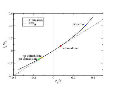
Figure 1: Binding momentum as a function of the inverse scattering length for a gaussian potential, both multiplied by the effective range $r_{e}$. Experimental data of four real systems are shown by the filled circles.

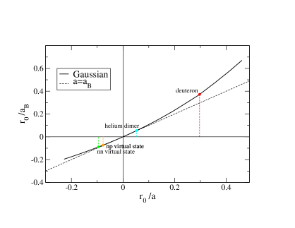
Figure 2: Binding momentum as a function of the inverse scattering length for a gaussian potential, both multiplied by the gaussian range $r_{0}$. Data of real systems are located in the plot through the ratio $a/a_{B}$.

III The three-body case

III.1 Three equal bosons

Inside the unitary window the three-boson $s$-wave spectrum has a particular form as was deduced for the first time by V. Efimov efimov1 ; efimov2 . In the case of zero-range interactions the system is unbounded from below; this property is known as the Thomas collapse thomas . Moreover the CSI is broken and the residual symmetry is the discrete scale invariance (DSI). The physics is invariant under the rescaling $r\rightarrow\Lambda^{n}r$, where the constant is usually written $\Lambda=\text{e}^{\pi/s_{0}}\approx 22.7$, with $s_{0}\approx 1.00624$ an universal number characterizing the three-identical boson system. At the unitary limit the spectrum consists of a geometrical series of states which accumulate at zero energy with ratio between two consecutive energy states $E_{3}^{(n+1)}/E_{3}^{(n)}=\text{e}^{-2\pi/s_{0}}$. This effect is known as the Efimov effect. Many experimental efforts have been done to study this scenario using atomic traps  kraemer2006 ; zaccanti2009 ; ferlaino2011 ; matchey2012 ; roy2013 ; cornell2017 . As the system moves away from the unitary limit the highest excited states disappear into the atom-dimer continuum one by one. A detailed analysis of three-boson spectrum for systems having a large scattering length can be found in the reviews by Braaten and Hammer report and by Naidon and Endo naidon . A discussion of these systems within the EFT framework can be found in Refs. vankolck1 ; vankolck2 whereas in Ref. gatto2019 a detailed parametrization of the zero-range universal function has been done. When the Schrödinger equation is solved using a regular, finite-range, potential located at unitarity, i.e. when there is a two-body bound state at threshold, the three-body system is bound from below (the Thomas collapse is not present anymore). However an infinite number of excited states appear above the ground state showing the Efimov effect. Though there are some range effects in the energy ratios for the lowest states, the constant ratio of $\approx 22.7^{2}$ can be seen for ratios calculated between consecutive higher states.

We proceed to the characterization of the unitary window for three particles in the same way as for the two-body system. We solve the Schrödinger equation for three equal mass bosons interacting through a gaussian potential. The first two levels are shown in Fig.3 where the three-body binding momenta $\kappa^{(n)}_{3}=\sqrt{m|E^{(n)}_{3}|/\hbar^{2}}$ for $n=0,1$ have been calculated as a function of the two-body binding momentum $\kappa_{2}=1/a_{B}$, both multiplied by the gaussian range $r_{0}$ to build dimensionless quantities. At the unitary limit the pure numbers $\kappa_{*}^{(n)}r_{0}$, indicated in the figure for $n=0,1$, are the same for all gaussian potentials. The energy goes quadratically to $\infty$ as $r_{0}\rightarrow 0$, a simple way to illustrate the Thomas collapse. The ratio of the first two levels, $\kappa_{*}^{(0)}/\kappa_{*}^{(1)}=22.98$ shows a small range effect. If we consider the third level, $n=2$, (not shown in the figure), we obtain $\kappa_{*}^{(2)}r_{0}=0.0009362$, and the ratio $\kappa_{*}^{(1)}/\kappa_{*}^{(2)}=22.70$ is almost equal to the universal ratio.

As the system moves from the unitary limit towards the positive region the infinite tower of excited states disappear one by one into the $1+2$ continuum crossing the two-body threshold, shown in the plot by the solid red curve. The second and third excited states are the last ones to cross the threshold around the values $r_{0}/a_{B}=0.013$ and $0.00069$, respectively. These pure numbers are the same for all gaussian potentials. The ground state and the first excited state do not cross the threshold; they form a two-level structure already observed in the helium trimer kunitski . The two levels of the helium trimer are located on Fig.3 (solid squares) through the angle defined by $\kappa^{(n)}_{3}a_{B}=\tan\xi_{n}$. Using the LM2M2 potential to describe those states, the position on the $r_{0}/a_{B}$ axis is not the same for both levels. It is 0.0612 for the ground state and 0.0637 for the first excited state, using the values given in Table I, the following gaussian radius can be extracted: $r_{0}^{(0)}=11.15\;a_{0}$ and $r_{0}^{(1)}=11.70\;a_{0}$, respectively. With the former range the gaussian potential describes simultaneously the dimer and trimer ground state energies whereas with the latter the dimer and the first excited state energies. With the values of $r_{0}^{(0)}$ we can predict the binding energy values of the two levels at unitarity

$$E_{*}^{(0)}=\frac{\hbar^{2}}{m}\left[\kappa_{*}^{(0)}\right]^{2}=\frac{\hbar^{2}}{m}\left[\frac{0.4883}{r_{0}^{(0)}}\right]^{2}=83.0\;{\rm mK}$$ (6)

$$E_{*}^{(1)}=\frac{\hbar^{2}}{m}\left[\kappa_{*}^{(1)}\right]^{2}=\frac{\hbar^{2}}{m}\left[\frac{0.02125}{r_{0}^{(0)}}\right]^{2}=0.157\;{\rm mK}$$ (7)

to be in a good agreement with the values given in the literature for the LM2M2 potential when its strength is reduced in order to locate the two-body bound state at threshold barletta ; hiyama2014 .

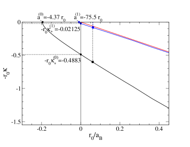
Figure 3: Three-body binding momentum as a function of the two-body binding momentum for a gaussian potential, both multiplied by the gaussian range $r_{0}$ to build dimensionless quantities. Notable points are indicated as solid circles as explained in the text.

Decreasing the strength of the gaussian potential the system enters the region of negative $a$ in which two particles are not bound. In this case $a_{B}$ is related to the energy of the two-body virtual state. At some point the first excited state of the trimer disappears into the three-atom continuum. Decreasing further the strength the interaction cannot bind the three particles and the ground state disappears too. The two-body scattering lengths at which these transitions occurs, indicated as $a_{-}^{(1)}$ and $a_{-}^{(0)}$ respectively, are shown by solid circles on top of Fig.3 in units of the gaussian range. Using the characteristic gaussian range, $r^{(n)}_{0}$, we can predict the values of the scattering length at threshold for the LM2M2 potential as $a_{-}^{(0)}\approx-48.7\;a_{0}$ and $a_{-}^{(1)}\approx-842\;a_{0}$ to be compared to $a_{-}^{(0)}\approx-48.2\;a_{0}$ and $a_{-}^{(1)}\approx-832\;a_{0}$ given in Ref. hiyama2014 .

This analysis demonstrates that the gaussian characterization of the states around the unitary window captures the essential ingredients of the dynamics. A more stringent test beyond the study of helium trimers is given by the almost model independent product $a_{-}^{(0)}\kappa_{*}^{(0)}\approx-2.2$ obtained through an analysis of experimental data for different van der Waals potentials having a repulsive core and supporting one or more bound states (see Ref.naidon and references therein). Surprisingly the gaussian potential predicts the values

$$a_{-}^{(0)}\kappa_{*}^{(0)}=-2.14$$ (8)

$$a_{-}^{(1)}\kappa_{*}^{(1)}=-1.56$$ (9)

capturing properties related to the van der Waals tail in the case of ground state level. In the case of the first excited state the product $a_{-}^{(1)}\kappa_{*}^{(1)}$ is close to the product obtained in zero-range limit ($a_{-}\kappa_{*}=1.507$, see Ref. aminus ) showing the minor size of the finite-range corrections in this state. The analysis of the $n=2$ level gives results comparable to the zero-range corrections at the $0.1\%$ level or better raquel . Within the EFT framework the results for the ground state can be considered at the level of next-to-leading order (NLO) whereas those for the excited state at LO level.

Another observable we can study using the gaussian characterization of the universal window is the atom-dimer scattering length. As derived by Efimov efimov3 , this observable has a universal expression in the zero-range limit

$$a_{AD}/a_{B}=d_{1}+d_{2}\tan[s_{0}\ln(\kappa_{*}a_{B})+d_{3}]\,,$$ (10)

where $d_{1}$, $d_{2}$ and $d_{3}$ are universal numbers and $\kappa_{*}$ is the three-body parameter labeling one three-body branch. This is a particular realization of the DSI with the log-periodic functional form and accordingly, as $a_{B}\rightarrow\infty$, the ratio $a_{AD}/a_{B}$ repeats its values forming different branches with asymptotes in the points in which the excited states disappear into the atom-dimer continuum. It should be noticed that a numerical analysis of the above form is very delicate due to the extremely weak binding of the dimer as $a_{B}\rightarrow\infty$. Here we analyze the behavior of $a_{AD}$ inside the unitary window for a gaussian potential up to the region in which the third excited state is present. The results are given in Fig.4 where much of the results presented in this section are collected. The (blue) solid circles are the numerical results of $a_{AD}/a_{B}$, obtained solving the zero-energy scattering problem, as a function of $r_{0}/a_{B}$. Presented in this way the results are the same for all gaussian potentials at the same $r_{0}/a_{B}$ value. The (blue) solid line has been obtained using the following parametrization of the function

$$a_{AD}/a_{B}=d_{1}+d_{2}\tan[s_{0}\ln(\kappa^{(1)}_{*}r_{0}(a_{B}/r_{0})+\Gamma_{3}^{(1)})+d_{3}]\,,$$ (11)

where we have used the pure number, $\kappa^{(1)}_{*}r_{0}=0.02125$, as the driving term and we have introduced the corresponding shift $\Gamma_{3}^{(1)}$, as discussed in Ref. gatto2013 . A reasonable fit to the calculations is obtained with $d_{1}=1.541$, $d_{2}=-2.080$, $d_{3}=-2.038$ and $\Gamma_{3}^{(1)}=0.061$. The two vertical dashed lines, located at $r_{0}/a_{B}=0.013$ and $0.00069$, are the asymptotes indicating the values at which the second and third excited states disappear into the atom-dimer threshold, respectively. From the figure we can see that the gaussian characterization of the $a_{AD}/a_{B}$ function has the log-periodic form in which the finite-range corrections have been absorbed in the shift parameter $\Gamma_{3}^{(1)}$.

In Fig.4 the position of the excited state of the trimer (lower red diamond) on the $n=1$ level, as given by the LM2M2 potential, is shown. Extending the corresponding value of the axis $r_{0}/a_{B}=0.0637$ to cross the $a_{AD}/a_{B}$ curve the value $a_{AD}/a_{B}=1.19$ is extracted. Therefore the gaussian characterization of the unitary window indicates, for that value of the $r_{0}/a_{B}$ ratio, the atom-dimer scattering length to be $a_{AD}=1.19\,a_{B}$. Using the LM2M2 value, $a_{B}=182.22\,a_{0}$, we obtain $a_{AD}=217\,a_{0}$, to be compared to the LM2M2 value for this quantity of $218.4\,a_{0}$ carbonell . So, a gaussian potential constructed to describe simultaneously the dimer and excited state of the trimer reproduces also the value of the atom-dimer scattering length within a $1\%$ error.

To analyse further the size of the finite-range effects the numerical value of $a_{AD}$ can be extracted from the higher branch of the $a_{AD}/a_{B}$ curve, between the two asymptotes shown in the Fig.4. To this aim the curve has to be evaluated at the coordinate $r_{0}/a_{B}$ corresponding to the position of trimer excited state on the third energy level ($n=2$). That point has coordinates $(r_{0}\kappa,r_{0}/a_{B})$ verifying $\kappa\,a_{B}=\tan\xi_{1}$, the same angle of the point on the $n=1$ level, indicated by the lower red diamond on the figure. The coordinate is $r_{0}/a_{B}=0.000239$ and corresponds to the value $a_{AD}/a_{B}=1.17$ giving $a_{AD}\approx 213\,a_{0}$. As for bound states, the result obtained using the lower branch can be considered at NLO level whereas using the higher branch at LO level.

This analysis shows that, inside the unitary window and in the low energy region, the complicate structure of the helium potential can be encoded in the strength and range of the a gaussian potential. The lowest energy state or branch, as in the case of atom-dimer scattering, captures the essential elements of system and can be considered at the NLO level in the EFT framework. The size of the corrections can be evaluated from the analysis of the higher states or branches and give results at the LO level. Moreover, varying the gaussian parameters a complete picture of the unitary window can be depicted.

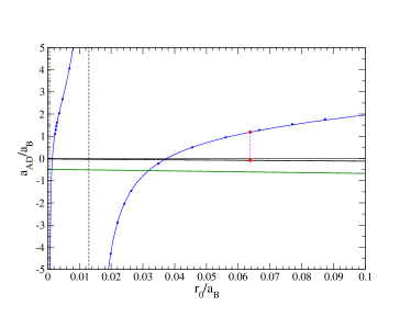
Figure 4: The atom-dimer scattering length (in units of $a_{B}$) as a function of the dimer binding momentum $\kappa_{2}=1/a_{B}$ times $r_{0}$. The blue solid points are the calculations using a gaussian potential and the blue solid line is the parametrization of Eq.(11). The binding momentum (times $r_{0}$) of the ground state (green solid line) and the first excited state (black solid line) are shown too. The solid red diamonds indicate the positions of the first excited state of the helium trimer and the atom-dimer scattering length. The two dashed lines indicate the position in which the second and third excited states cross the atom-dimer threshold.

III.2 Three $1/2$ spin-isospin fermions

We perform the gaussian characterization of the unitary window focusing on the three-nucleon system. The intention is to link the triton continuously to the unitary limit showing that particular characteristics of the three-nucleon system in the low-energy region are strictly related to its position in the unitary window. In particular we would like to explain the one-level structure of the triton, the almost zero value of the doublet neutron-deuteron scattering length $a_{nd}$, and the position of the triton virtual state indirectly observed through the $s$-wave phase shifts in low-energy neutron-deuteron scattering. Studies of the three-nucleon systems inside the unitary window can be found in Refs. kievsky2016 ; gatto2019b ; koenig ; kievsky2017 ; kievsky2018 .

To perform the gaussian characterization of the unitary window for the three-nucleon system we use a spin dependent gaussian interaction with different terms in both spin channels $S=0,1$

$$V(r)=V_{0}e^{-r^{2}/r_{0}^{2}}{\cal P}_{0}+V_{1}e^{-r^{2}/r_{1}^{2}}{\cal P}_{1}$$ (12)

where ${\cal P}_{0}$ and ${\cal P}_{1}$ are the projectors onto the spin-isospin channels $S,T=0,1$ and $1,0$ respectively. Moreover, we limit the two-body force to act in $s$-waves. The nuclear force is weak in angular momentum states $\ell>0$ and, in the low-energy region considered here, this restriction could be justified. In the study of the unitary window with such a force we consider the two gaussian ranges to be equal $r_{0}=r_{1}$. In this case, when $V_{0}$ is equal to $V_{1}$, the spectrum of total angular momentum and parity $J^{\pi}=1/2^{+}$ states is equivalent to the three-boson spectrum discussed previously.

Among different possibilities to characterize the unitary window, following Refs. kievsky2016 ; gatto2019b , we select trajectories maintaining constant the ratio of the singlet and triplet scattering lengths, $a_{0}$ and $a_{1}$, and equal to the nuclear physics value $a_{0}/a_{1}\approx-4.3$. With this condition, we vary the gaussian parameters to cover the plane $(-r_{0}\kappa_{3},r_{0}/a_{B})$, with $E_{3}=\hbar^{2}\kappa^{2}_{3}/m$ the three-body binding energy of the $J^{\pi}=1/2^{+}$ state and $E_{2}=\hbar^{2}/ma_{B}^{2}$ the two-body binding energy of the triplet state. The results are shown in the two panels of Fig.5 for discrete states and the zero-energy solution. The upper panel shows the $nd$ doublet scattering length ${}^{2}a_{nd}$, in units of the energy length $a_{B}$, as a function of $r_{0}/a_{B}$. In the negative region we show the binding momenta (times $r_{0}$) for the ground state (orange curve) and excited state (green curve) of the trimer. The dashed vertical line is the asymptote, at $r_{0}/a_{B}=0.101$, indicating the point in which ${}^{2}a_{nd}$ diverges and the trimer excited state disappears into the $1+2$ continuum. After the asymptote, the red curve shows the binding momentum of dimer (times $r_{0}$), in the $S=1$ state. The physical point, indicated by the red diamond on the trimer curve, has $\kappa_{3}a_{B}=\tan\xi=1.95$ corresponding to the square root of the ratio of the triton binding energy $8.48\,$MeV with the deuteron binding energy of $2.224\,$MeV. At that point $r_{0}/a_{B}=0.457$ and ${}^{2}a_{nd}/a_{B}=0.08$ allowing to extract the value of ${}^{2}a_{nd}=0.4\,$fm. This value is slightly lower of the experimental value ${}^{2}a_{nd}\approx 0.65\,$fm. However, the gaussian characterization is able to explain the almost zero value of this quantity if compared to the triplet $np$ scattering length $a_{1}=5.42\,$fm. This is a very delicate region in which slightly different values of $r_{0}/a_{B}$ produce large variations of ${}^{2}a_{nd}$, including a change of sign. The gaussian characterization places ${}^{2}a_{nd}$ in the correct (positive) region and shows the strong correlation between this quantity and the trimer energy observed already many years ago and known as the Phillips line phillips . As for the boson case it is possible to analyse the higher branch of the ${}^{2}a_{nd}/a_{B}$ curve to determine the size of finite-range corrections. To this aim the triton point is located on the $n=1$ level (green curve on the upper panel of Fig.5) at coordinates having the same value $\tan\xi=1.95$, this happens at $r_{0}/a_{B}=0.015$. At that coordinate ${}^{2}a_{nd}/a_{B}=0.06$, slightly lower than the value obtained analysing the $n=0$ level.

The lower panel of Fig. 5 shows calculations of the doublet scattering length ${}^{2}a_{nd}$ (solid blue circles) in a extended region and a fit to those values using the form of Eq.(11) (solid blue curve) with $d_{1}=0.542$, $d_{2}=-1.686$, $d_{3}=6.1952$, the shift $\Gamma_{3}^{(0)}=0.378$ and the driving term of the ground state energy $\kappa_{*}r_{0}=0.488$. Using the fit we can extract the asymptote at $r_{0}/a_{B}=0.101$ and determine the energy length at which the excited state disappears $a_{B}\approx 16\,$fm. This analysis explains the existence of one bound state for the three-nucleon system: at the physical values of $a_{0}$ and $a_{1}$ the excited state has crossed the threshold becoming a virtual state. Finally, using the value $r_{0}/a_{B}=0.457$ at the triton point and from the deuteron length, $a_{B}=4.32\,$fm, we can extract the characteristic gaussian range $r_{0}=1.97\,$fm from which it is possible to assign a value of the three-nucleon system at unitary through the quantity $\kappa_{*}r_{0}=0.488$. We obtain $E_{*}\approx 2.5\,$MeV in good agreement with previous estimates gatto2019b ; epelbaum .

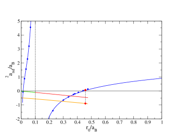
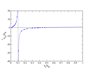
Figure 5: The doublet neutron-deuteron scattering length ${}^{2}a_{nd}$ in units of the triplet two-body energy length $a_{B}$ as a function of the inverse of $a_{B}$ in units of the gaussian range $r_{0}$ (blue solid points). The blue line is the parametrization of Eq.(11). In the upper panel the dimensionless binding momenta $\kappa^{(n)}_{3}r_{0}$ of the three-nucleon ground state (orange curve), $n=0$, and excited state (green curve), $n=1$, are shown together with the binding momentum $\kappa_{2}r_{0}$ of the two-body bound state (red curve). The excited state almost overlaps with the two-body state. The red diamonds indicate the physical point of the ground state curve and the corresponding value on the ${}^{2}a_{nd}$ curve. The lower panel shows ${}^{2}a_{nd}/a_{B}$ in a larger region. The vertical dashed line is the asymptote at which ${}^{2}a_{nd}$ diverges.

IV The three-body virtual states

We have studied the three-body energy spectrum inside the unitary window using a gaussian interaction with variable strength and we have observed that when the excited state cross the $1+2$ threshold the particle-dimer scattering length diverges and the excited state becomes a virtual state. Here we study the evolution of the virtual state after that crossing. For bosons we saw that the first excited state never crosses the threshold, the last level to cross the threshold is the second excited state quite close to the unitary limit and therefore it has little effects in low-energy atom-dimer collisions as the system moves away from the unitary limit. Conversely, we have observed that for fermions along the nuclear trajectory the first excited state crosses the threshold becoming a virtual state. As we will see, its position at the physical point could be determined from the low-energy neutron-deuteron scattering. To this respect, the virtual state of the triton has been subject of different studies for a long time, see Refs. fuda ; babenko , for a recent review see Ref. orlov and references therein whereas in Ref. higa a treatment within EFT is presented.

In order to determine the position of the virtual state we calculate the $s$-wave effective range function $S_{k}=k\cot\delta$, where $k$ is defined from the center of mass particle-dimer energy $E=3\hbar^{2}k^{2}/4m$ and $\delta$ is the corresponding phase shift. In the case of bosons

$$\lim_{k\rightarrow 0}S^{B}_{k}=-\frac{1}{a_{AD}}.$$ (13)

In the case of $1/2$ spin-isospin fermions we study neutron-deuteron scattering in the $J^{\pi}=1/2^{+}$ state with

$$\lim_{k\rightarrow 0}S^{F}_{k}=-\frac{1}{{}^{2}a_{nd}}.$$ (14)

The superscripts $B$ or $F$ in the effective range function identify the different symmetries. The effective range functions, calculated using a gaussian potential, are given in Fig.6 for different values of center of mass energy energies. In the figure the dimensionless quantities $a_{AD}S^{B}_{k}$ (upper panel) and ${}^{2}a_{nd}S^{F}_{k}$ (lower panel), for bosons and fermions, respectively, are shown as a function of $a_{B}k$. Using this form both functions start at $-1$ at zero energy and the breakup threshold is $a_{B}k=2/\sqrt{3}$. The different curves are labelled by the ratio $r_{0}/a_{B}$ and correspond to some of the $a_{AD}$ and ${}^{2}a_{nd}$ values given in Fig.4 and Fig.5. From the effective range function, or directly from the phase-shifts at different energies, it is possible to construct a representation of the $S-$matrix and extract the pole located at the negative imaginary axis (the virtual state).

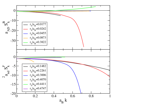
Figure 6: The effective range functions $S^{B}_{k}$ (upper panel) and $S^{F}_{k}$ (lower panel) as functions of the energy momentum $k$, multiplied by energy length $a_{B}$. The different curves correspond to different dimer binding energies.

Close to the $1+2$ threshold the virtual state can be detected through a particular form of the effective range function. Following Ref. orlov , the effective range function can be parameterized as

$$S_{k}^{\lambda}\approx\frac{-1/a_{\lambda}+C^{\lambda}_{2}k^{2}+C^{\lambda}_{4}k^{4}}{1+k^{2}/(k^{\lambda}_{0})^{2}}$$ (15)

with $\lambda=B,F$ and $a_{\lambda},C^{\lambda}_{2},C^{\lambda}_{4},k^{\lambda}_{0}$ parameters used to fit experimental values for phase-shifts or, when not available, numerical results using potential models. As discussed in Ref. orlov , these four quantities are related to the energy of the $S$-matrix pole, $E_{p}=-3\hbar^{2}k^{2}_{p}/4m$. One possibility to extract the virtual state in the unitary window using numerical results obtained with the gaussian potential would be to determine those four parameters. We found more convenient to use the gaussian phase-shifts directly to derive the Padé approximant representation of the $S$-matrix and extract the pole on the negative imaginary axis using the method given in Ref. elander . We have followed this technique and the quantities, $a_{AD}k_{p}$ and ${}^{2}a_{nd}k_{p}$, for three bosons or three-fermions along the nuclear plane, are given in Fig.7 as functions of $r_{0}/a_{B}$. In the boson case the pole has initially an almost linear behavior and moves away from the threshold. Conversely, in the three-nucleon case, the pole move smoothly and remains close to the threshold even at the physical point. This allows the possibility of its determination analyzing experimental data for $nd$ scattering close to threshold.

The position of the virtual state at the physical point for three-nucleons can be compared to values obtained from experimental results, which are not exhaustive, or to results obtained from realistic potential models. To analyse the latter possibility, we perform calculations for the three-nucleon system using two realistic forces, the CD Bonn potential including the $\Delta$-isobar excitation and the three-body force (CD-Bonn+D+U3) deltuva:15d and the AV18 potential with the Urbana IX force slightly modified to reproduce the triton binding energy and ${}^{2}a_{nd}$ (AV18+URIX’) kievsky2010 . Furthermore the spin-dependent two-body gaussian potential supplemented with a hyperradial three-body force (2BG+3BG) of the following form has also been used

$$V(i,j)+W(i,j,k)=V_{0}e^{-r^{2}/r_{0}^{2}}{\cal P}_{0}+V_{1}e^{-r^{2}/r_{1}^{2}}{\cal P}_{1}+W_{0}e^{-\rho^{2}/\rho_{0}^{2}}$$ (16)

with strength parameters $V_{0}=37.9\,$ MeV, $V_{1}=60.575\,$ MeV, $W_{0}=2.7947\,$MeV and range parameters $r_{0}=r_{1}=1.65\,$fm and $\rho_{0}=5.05\,$fm. With this selection the two- and three-body low-energy quantities are well described including the triton binding energy and ${}^{2}a_{nd}$. The nuclear physics point corresponds to $r_{0}/a_{B}=0.457$ and the results of these realistic models lie almost on the gaussian curve. For the three models, the $s$-wave $J^{\pi}=1/2^{+}$ low-energy phase shifts are shown in Fig.8 from which the energy of the pole $E_{p}=0.48\,$MeV can be extracted. The three pole energy values are indicated in Fig.7. As can be seen from the figure, the gaussian characterization describes correctly this state.

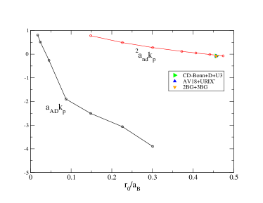
Figure 7: The virtual state pole momentum for three bosons and three fermions for different dimer energies. The realistic cases for fermions are on top of the gaussian characteristic curve.

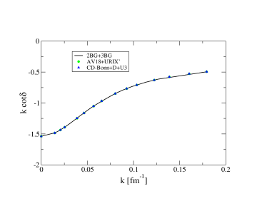
Figure 8: The effective range function for the three realistic cases discussed.

V Conclusions

Due to the independence on the interaction details, few-body systems have been studied inside the unitary window interacting through a gaussian potential. This research follows other studies that can be found in Refs. kievsky2014 ; bazak ; artur ; artur1 . In the present study we perform a step further constructing a gaussian characterization of the unitary window for different observables in the three-body sector. The aim of this study is twofold; from one side we would like to extend the characterization of the unitary window from the zero-range theory to finite range. One the other side we would like to use the gaussian trajectories to analyze universal behavior. Many properties of real systems are well described using detailed interaction models, we refer for example to realistic He-He or $NN$ interactions. Since these interactions are determined from a set of experimental data, when a system is forced to move from its phyiscal point the original interaction is modified in a certain (unknown) form. Broad Feshbach resonances used to explore the unitary window are compatible with an overall strength multiplication of the atomic potential. Essentially this kind of process is well represented by a gaussian potential with variable strength and fixed range. If the evolution of a system inside the unitary window follows the gaussian trajectories we identify this system as a representative of the universal class of weakly bound systems; in fact, a unique gaussian range can be identified and used to accommodate observables, as binding energies, on top of the gaussian trajectories. In this way very different systems have been mapped on the same curve identifying their universal behavior. To this respect the gaussian trajectories make one step further with respect to the zero-range trajectories since they include range corrections.

Firstly, following the above methodology, we have studied the two-body system; we have placed on the gaussian curve four different systems, the helium dimer, the deuteron and the $S=0$ $np$ and $nn$ systems. The position on the curve can be used as a measure of the distance of the physical point from the unitary limit. Then, we have characterized the three-body system inside the unitary window; in the case of three-equal bosons, focusing on the system of three helium atoms, and in the case of three $1/2$ spin-isospin fermions, focusing on the three-nucleon system. Using a gaussian potential we have studied the energy spectrum, bound and excited states, and $s$-wave low-energy scattering. The next step has been to map on the gaussian trajectories the physical points and to identify correlations between the observables. These correlations, used as a signal of universality, has been found to be very effective. From the location of the physical points we have been able to predict the values of the corresponding $1+2$ scattering lengths. The helium atom-dimer scattering length has been predicted with a good accuracy. In the case of the doublet neutron-deuteron scattering length an approximate value has been extracted, however the correct position close to zero has been correctly predicted. In the former case, the almost independent product $a^{(0)}_{-}\kappa_{*}^{(0)}$ has been found to coincide closely to the value of different van der Waals species, giving a further confirmation of the potentialities of using gaussian trajectories to identify universal behavior. Using the (approximate) DSI we have analysed the higher energy levels or branches, in the case of atom-dimer or deuteron-neutron scattering length, to assess the size of finite-range corrections. In the framework of EFT, the results obtained from the lowest energy level or branch can be considered at NLO whereas the higher ones, very close to the zero-range interaction model, represent LO results.

In the final part we have studied the virtual states appearing when the excited states cross the $1+2$ threshold. This is particularly interesting in the three-nucleon system where the virtual state of the triton has been subject of many investigations. From our analysis the virtual state is located at $E_{p}=-0.48\,$ MeV, consistently with previous determination orlov . The analysis presented in our work is useful to characterize low-energy properties of few-nucleon systems as belonging to the universal window. In conclusion, when a system is located inside the unitary window, the ratio of the three- and two-body energies determines the angle from which the system is placed on the trajectory and determines the characteristic gaussian range. Then the gaussian potential with that range can be used to perform a complete characterization of the universal window for that system. Other observables strictly correlated to the binding energy can be predicted as well. In this way we can study scale symmetries observed in the real systems as continuously linked to the unitary point, a point in which those symmetries are well verified bira2017 .

References

- (1) H.A. Bethe, Phys. Rev. 76, 38 (1949)
- (2) P.F Bedaque, H.-W. Hammer, and U. van Kolck, Phys. Rev. Lett. 82, 463 (1999).
- (3) P. Bedaque, H.-W. Hammer, and U. van Kolck, Nucl. Phys. A 676, 357 (2000).
- (4) M. Gattobigio and A. Kievsky, Phys. Rev A 90, 012502 (2014).
- (5) R. Álvarez-Rodríguez, A. Deltuva, M. Gattobigio and A. Kievsky, Phys. Rev. A 93, 062701 (2016).
- (6) A. Kievsky and M. Gattobigio, Few-Body Syst. 57, 217 (2016)
- (7) M. Gattobigio, A. Kievsky, and M. Viviani, Phys. Rev. C 100, 034004 (2019).
- (8) V. Efimov, Phys. Leet. B 33, 563 (1970)
- (9) V. Efimov, Yad. Fiz. 12, 1080 (1970) [Sov. J. Nucl. Phys. 12, 589 (1971)]
- (10) A. Deltuva and P. U. Sauer, Phys. Rev. C 91, 034002 (2015)
- (11) A. Kievsky, Nucl. Phys. A624, 125 (1997)
- (12) A. Kievsky, S. Rosati, M. Viviani, L. E. Marcucci and L. Girlanda, , J. Phys. G: Nucl. Part. Phys. 35, 063101 (2008)
- (13) R.A. Aziz and M.J. Slaman, J. Chem. Phys. 94, 8047 (1991)
- (14) L.H. Thomas, Phys. Rev. 47, 903 (1935)
- (15) T. Kraemer et al., Nature 440, 315 (2006).
- (16) M. Zaccanti et al., Nat. Phys. 5, 586 (2009).
- (17) F. Ferlaino et al., Few-Body Syst. 51, 113 (2011).
- (18) O. Matchey, Z. Shotan, N. Gross, and L. Khaykovich, Phys. Rev Lett. 108, 210406 (2012).
- (19) S. Roy et al., Phys. Rev Lett. 111, 053202 (2013).
- (20) C. E. Klauss et al., Phys. Rev Lett. 119, 143401 (2017).
- (21) E. Braaten and H.-W. Hammer, Phys. Rep. 428, 259 (2006).
- (22) P. Naidon and S. Endo Rep. Prog. Phys. 80 056001 (2017)
- (23) M. Gattobigio, M. Göbel, H.-W. Hammer and A. Kievsky, Few-Body Syst. 60, 40 (2019)
- (24) M. Kunitski et al., Science 348, 551 (2015).
- (25) P. Barletta and A. Kievsky, Phys. Rev. A 64, 042514 (2001).
- (26) E. Hiyama and M. Kamimura, Phys. Rev A 90, 052514 (2014)
- (27) A. O. Gogolin, C. Mora and R. Egger, Phys. Rev. Lett. 100, 140404 (2008).
- (28) V. Efimov, Yad. Fiz. 29, 1058 (1979) [Sov. J. Nucl. Phys. 29, 546 (1979)]
- (29) A. Kievsky and M. Gattobigio, Phys. Rev. A 87, 052719 (2013).
- (30) J. Carbonell, A. Deltuva, and R. Lazauskas, Comp. Rend. Phys. 12, 47 (2011)
- (31) A.C. Phillips, Nucl. Phys. A 107, 209 (1968)
- (32) E. Epelbaum, H.-W. Hammer, U.-G. Meißner, and A. Nogga, Eur. Phys. J. C48, 169 (2006)
- (33) B.A. Girard and M.G. Fuda, Phys. Rev. C 19, 579 (1979)
- (34) V.A. Babenko and N.M. Petrov Yad. Fiz. 63, 1798 (2000) [Phys. At. Nucl. 63, 1709 (2000)]
- (35) Yu.V. Orlov and L.I. Nikita, Yad. Fiz. 69, 631 (2006) [Phys. At. Nucl. 69, 607 (2005)]
- (36) G.Rupak, A. Vaghani, R. Higa, and U. van Kolck, Phys. Lett. B 791, 414 (2019)
- (37) S.A. Rakityansky, S.A. Sofianos, and N. Elander, J. Phys. A: Math. Theor. 40, 14857 (2007)
- (38) A. Kievsky, M. Viviani, L. Girlanda, and L.E. Marcucci, Phys. Rev. C81, 044003 (2010)
- (39) S. König, H.W. Grießhammer, H.-W. Hammer, and U. van Kolck, Phys. Rev. Lett. 118, 202501 (2017).
- (40) A. Kievsky, M. Viviani, M. Gattobigio, and L. Girlanda, Phys. Rev. C95, 024001 (2017)
- (41) A. Kievsky, M. Viviani, D. Logoteta, I. Bombaci, and L. Girlanda, Phys. Rev. Lett. 121, 072701 (2018)
- (42) A. Kievsky, N.K. Timofeyuk, and M. Gattobigio, Phys. Rev, A90, 032504 (2014).
- (43) B. Bazak, M. Eliyahu, and U. van Kolck, Phys. Rev. A94, 052502 (2016)
- (44) A. Kievsky, A. Polls, B. Juliá Díaz, and N.K. Timofeyuk, Phys. Rev A 96, 040501(R) (2017)
- (45) A. Kievsky, A. Polls, B. Juliá Díaz, N.K. Timofeyuk, and M. Gattobigio, submitted for publication.
- (46) U. van Kolck, Few-Body Syst. 58, 112 (2017)