Model of heat diffusion in the outer crust of bursting neutron stars

Abstract

We study heat diffusion after an energy release in a deep spherical layer of the outer neutron star crust ($10^{7}\lesssim\rho\lesssim 4\times 10^{11}$ g cm^-3). We demonstrate that this layer possesses specific heat-accumulating properties, absorbing heat and directing it mostly inside the star. It can absorb up to $\sim 10^{43}-10^{44}$ erg due to its high heat capacity, until its temperature exceeds $T\sim 3\times 10^{9}$ K and triggers a rapid neutrino cooling. A warm layer ($T\sim 10^{8}-3\times 10^{9}$ K) can serve as a good heat reservoir, which is thermally decoupled from the inner crust and the stellar core for a few months. We present a toy model to explore the heat diffusion within the heat-accumulating layer, and we test this model using numerical simulations. We formulate some generic features of the heat propagation which can be useful, for instance, for the interpretation of superbursts in accreting neutron stars. We present a self-similar analysis of late afterglow after such superbursts, which can be helpful to estimate properties of bursting stars.

1 Introduction

Many neutron stars demonstrate bursting activity. For instance, accreting neutron stars in low-mass X-ray binaries show X-ray bursts and superbursts powered by explosive burning of accreted hydrogen and helium in surface layers and subsequent more powerful burning of carbon in deeper layers (e.g., in ’t Zand 2017; Galloway & Keek 2017). These processes involve complicated physics of thermal evolution of accreting neutron stars, steady-state and explosive nuclear burning with extended reaction networks, various mass and heat transport mechanisms (hydrodynamical motions, convection, thermal diffusion) and so on.

We mainly focus on heat diffusion after energy generation in deep layers of the outer crust of neutron stars. Such a process has been extensively simulated numerically and semi-analytically for about two decades in the context of modeling superbursts; see, e.g. Cumming & Macbeth (2004); Cumming et al. (2006); Keek & Heger (2011); Altamirano et al. (2012); Keek, Heger & in ’t Zand (2012); Keek et al. (2015) and references therein.

The outer crust (e.g. Haensel, Potekhin & Yakovlev 2007) is a relatively thin layer which extends from the stellar surface to the neutron drip density ($\rho_{\text{drip}}\approx 4.3\times 10^{11}$ g cm^-3). Its width is only some hundred meters, and its mass is $\sim 10^{-5}$ $\textrm{M}_{\odot}$. It consists of electrons and ions (atomic nuclei). We call it crust for simplicity; actually, the atomic nuclei can constitute either Coulomb solid, or Coulomb liquid or gas, depending on density $\rho$, temperature $T$ and nuclear composition (our ‘crust’ includes thus the liquid ‘ocean’). We consider a spherically symmetric star, neglecting the effects of magnetic fields and rotation. We will mainly study heat propagation at

$$\rho_{\text{b}}\lesssim\rho\lesssim\rho_{\text{drip}},\leavevmode\nobreak\ \leavevmode\nobreak\ 10^{8}\lesssim T\lesssim 3\times 10^{9}\leavevmode\nobreak\ {\rm K},$$ (1)

where $\rho_{\text{b}}\sim 10^{7}$ g cm^-3 (so that the electrons are relativistic and strongly degenerate), and the ions are fully ionized. Lower $T$ are less interesting as far as the processes of energy release are concerned (typical ignition temperatures for deep nuclear explosions are not so low). We will analyse specific heat-accumulating properties of these layers.

In our previous studies (e.g. Kaminker et al. 2014; Chaikin, Kaminker & Yakovlev 2018, and references therein) we have simulated the heat propagation in a neutron star after some energy release in its crust (in 1D and 2D geometries, with the heater placed within a spherical layer or some spot-like region). There we have mainly considered the heaters that operate quasi-statically over months or longer, corresponding either to hypothetical energy release in the crust of magnetars or to the outbursts (accretion periods) in soft X-ray transients.

Here we study the heaters that are active on time-scales of minutes that is closer to the individual X-ray bursts or superbursts on neutron stars. Our aim is to present a simplified model of heat diffusion and test it using a modern thermal evolution code. The model reproduces and elucidates generic properties of deep superbursts and enables one to estimate how these properties depend on system parameters, particularly on neutron star mass and radius.

In Sections 2 and 3 we formulate a simplified model for studying heat diffusion in the $\rho-T$ domain (1) and discuss its formal semi-analytic solution for an instant burst in a thin layer. Section 4 is devoted to bursting layers of finite width in domain (1), and Section 5 to bursts in similar layers but extended to lower densities. We compare analytic solutions with numerical models. In Section 6 we discuss generic features of heat diffusion after bursts. In Section 7 we analyse late burst decay and present a simple method for evaluating parameters of bursting neutron stars from observations of such decays. We conclude in Section 8, and present some technical details in Appendix A.

2 Simplified analytic model of heat diffusion

2.1 Basic parameters and microphysics

We introduce a simplified ‘toy’ model of a spherically symmetric outer crust of the neutron star in the $\rho-T$ domain (1). The crust is thin and can be regarded as locally flat (e.g. Gudmundsson et al. 1983). Unless the contrary is indicated, we will use this locally flat coordinate system. Let $z$ be a proper depth measured from the neutron star surface ($z=0$). The density $\rho$ can be conveniently expressed through the relativity parameter of degenerate electrons (Salpeter, 1961), $x_{\text{r}}=p_{\text{F}}/(m_{\text{e}}c)\approx 1.0088(\rho_{6}Z/A)^{1/3}$, where $\rho_{6}=\rho/(10^{6}\leavevmode\nobreak\ \mbox{g\leavevmode\nobreak\ cm${}^{-3}$})$, $p_{\text{F}}$ is the electron Fermi momentum; $A$ and $Z$ are the mean ion mass and charge numbers, respectively. The $A/Z$ ratio is assumed to be constant throughout the outer crust. With these assumptions, the density profile $\rho(z)$ is determined by (Haensel, Potekhin & Yakovlev, 2007)

$$x_{\text{r}}^{3}=\left[\frac{z}{z_{0}}\,\left(2+\frac{z}{z_{0}}\right)\right]^{3/2}\approx\left(\frac{z}{z_{0}}\right)^{3},$$ (2)

with $z_{0}=(Zm_{\text{e}}c^{2})/(m_{\text{u}}g_{\text{s}}A)$ and $g_{\text{s}}=(GM/R^{2})(1-r_{\text{g}}/R)^{-1/2}$ ( $m_{\text{u}}$ being the atomic mass unit). Here, $g_{\text{s}}$ is the local gravitational acceleration in the outer crust, which is nearly constant there and is expressed through the gravitational mass of the star $M$ and its circumferential radius $R$; $z_{0}$ is a characteristic depth of the outermost layer ($\rho\lesssim 10^{6}$ g cm^-3) in which the degenerate electrons are non-relativistic; $r_{\text{g}}=2GM/c^{2}$ is the gravitational radius of the star. The last expression in equation (2) is the asymptote at depths $z\gg z_{0}$, where the electrons are degenerate and ultra-relativistic; it will be used below in the toy-model analysis. In particular, it gives the column density $y=z\rho/4$; it becomes inaccurate at $\rho\lesssim\rho_{\text{b}}$.

The diffusion of heat through the envelope in question is described by the equation

$$C{\partial\over\partial t}\ T-{\partial\over\partial z}\left(\kappa{\partial\over\partial z}\ T\right)=Q,$$ (3)

where $T$ is the local (non-redshifted) temperature, $\kappa$ is the thermal conductivity, $C$ is the heat capacity per unit volume at constant pressure, and $Q$ is the energy generation rate per unit volume. Since the electron gas is strongly degenerate, the heat capacities at constant volume and pressure are sufficiently close. We assume also that thermal processes do not violate hydrostatic equilibrium ($\partial P/\partial z=g_{\text{s}}\rho$, where $P$ is the pressure dominated by the relativistic degenerate electrons).

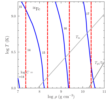
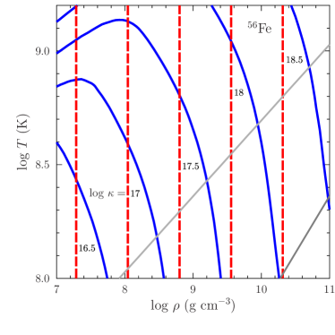
Figure 1: Isolines of constant heat capacity $C$ [$k_{\text{B}}$ cm^-3] (the left-hand panel) and thermal conductivity $\kappa$ [erg cm^-1 s^-1 K^-1] (the right-hand panel) in the $T-\rho$ plane for iron matter. Solid lines are accurate values, dashed lines refer to the toy-model approximation. The numbers show the values of log $C$ and log $\kappa$. See the text for details.

In reality, $C$, $\kappa$ and $Q$ depend both on density and on temperature, which makes equation (3) non-linear. In the numerical simulations we take these dependences into account. In the toy model, we linearize equation (3) by assuming that $C$ and $\kappa$ are temperature-independent (which is a reasonable approximation, as we argue below) and that the dependence of energy release on depth and time, $Q(z,t)$, is given explicitly.

In the given $\rho-T$ region (1) one can suggest two major approximations of $C$ and $\kappa$. Since the electrons are strongly degenerate, the heat capacity is mainly determined by the ions. In an ideal classical crystal, the ion heat capacity is $C_{\text{i}}=3n_{\text{i}}\mbox{$k_{\text{B}}$}$, where $k_{\text{B}}$ is the Boltzmann constant. Quantum effects strongly reduce $C_{\text{i}}$ at $T\ll T_{\text{pi}}$, where $T_{\text{pi}}=\hbar\omega_{\text{pi}}/\mbox{$k_{\text{B}}$}\approx 7.8\times 10^{6}\sqrt{\rho_{6}}\,(Z/A)$ K and $\omega_{\text{pi}}$ is the ion plasma frequency. However, in real strongly coupled, strongly degenerate non-ideal Coulomb plasma (liquid or crystal), the total heat capacity per ion remains close to $3\mbox{$k_{\text{B}}$}$ in a wide range of temperatures around the melting line $T_{\text{m}}\sim 2.3\times 10^{7}(Z/26)^{2}(A/56)^{-1/3}\rho_{6}^{1/3}$ K (e.g., Haensel et al. 2007, Section 2.4.6). Bearing in mind an approximate nature of our analysis, we take

$$C\approx 3\mbox{$k_{\text{B}}$}n_{\text{i}}=az^{3},\quad a\approx\frac{\mbox{$k_{\text{B}}$}}{Z\pi^{2}}\,\left(\frac{m_{\text{e}}c}{\hbar z_{0}}\right)^{3},$$ (4)

where we use $n_{\text{i}}=n_{\text{e}}/Z$ due to electric neutrality of the matter. In this approximation, $C$ is temperature-independent and proportional to $\rho$.

The thermal conductivity $\kappa$ is mainly provided by strongly degenerate electrons, which scatter off ions (off ion-charge fluctuations, to be exact). It is determined by the familiar expression (e.g., Ziman, 1960) $\kappa=\pi^{2}k_{\text{B}}^{2}Tn_{\text{e}}\tau_{\text{eff}}/(3m_{\text{e}}^{*})$, where $\tau_{\text{eff}}$ is the effective electron relaxation time and $m_{\text{e}}^{*}=m_{\text{e}}\,/\sqrt{1-v_{\text{F}}^{2}/c^{2}}$ is the effective electron mass, $v_{\text{F}}=cx_{\text{r}}/\sqrt{1+x_{\text{r}}^{2}}$ being the electron Fermi velocity. For $\tau_{\text{eff}}$, we employ an estimate (Yakovlev & Urpin, 1980),

$$\frac{1}{\tau_{\text{eff}}}=\frac{e^{2}}{\hbar v_{\text{F}}}\,\left(2-\frac{v_{\text{F}}^{2}}{c^{2}}\right)\,\frac{\mbox{$k_{\text{B}}$}Tu_{-2}}{\hbar},$$ (5)

where $u_{-2}\approx 13$ is a frequency moment of phonon spectrum in a Coulomb crystal of ions. This estimate is obtained for electrons, which scatter off phonons at $T\gtrsim T_{\text{pi}}/5$. It neglects quantum effects in ion motions and multi-phonon scattering processes (Baiko et al., 1998). It stays roughly valid in a strongly coupled Coulomb liquid of ions. In our case, it is sufficient to use the relativistic limit ($v_{\text{F}}\to c$), in which case

$$\kappa\approx bz^{2},\quad b=\frac{\zeta\mbox{$k_{\text{B}}$}c^{4}m_{\text{e}}^{2}}{9e^{2}\hbar u_{-2}z_{0}^{2}}.$$ (6)

Then $\kappa$ is independent of $T$ and $b$ is a constant. Here, we introduce a phenomenological constant correction factor $\zeta$ which makes our approximation of $\kappa$ more consistent with advanced calculations (Potekhin et al., 1999). For the iron plasma to be considered below we set $\zeta=1/4$.

Substituting (4) and (6) into equation (3), we have

$$az^{3}{\partial\over\partial t}\ T-b{\partial\over\partial z}\left(z^{2}{\partial\over\partial z}\ T\right)=Q(z,t).$$ (7)

This is our basic toy-model equation, which is linear in $T$ and can be solved by standard methods of mathematical physics as we discuss later.

The accuracy of our approximations (4) and (6) is demonstrated in Fig. 1. It shows isolines of constant $C$ and $\kappa$ (the left-hand and right-hand panels, respectively) in the $T-\rho$ plane. For illustration, here and below we use the model of the outer neutron star crust composed of iron. We have chosen iron as a leftover of nuclear burning of light elements. The numbers next to the lines give the values of decimal logarithms $\log C$ and $\log\kappa$. The vertical dashed lines are our approximations. The solid lines are based on numerically accurate values of $C$ and $\kappa$. Accurate $C$ includes the contribution of ions, electrons, photons, as well as of electron-positron pairs. Accurate $\kappa$ includes the contribution of electron-ion and electron-electron collisions and also of radiative conduction. To guide the eye, the two gray lines show two characteristic temperatures (e.g. Haensel et al. 2007) as functions of $\rho$. The lighter line is the melting temperature $T_{\text{m}}$ of the classical Coulomb crystal of iron ions. The darker line is $T_{\text{pi}}/5$. Below this line, quantum effects in ion motion substantially suppress the heat capacity of the ions.

According to Fig. 1, our approximations of $C$ and $\kappa$ seem reasonable. Deviations of accurate and toy model heat capacities at $\rho\lesssim 10^{7}$ g cm^-3 and $T\gtrsim 3\times 10^{8}$ K are mainly due to the contribution of electrons and photons in the accurate $C$ (the electron degeneracy becomes reduced which makes the electron and radiative heat capacities more important). The deviations at $\rho\gtrsim 3\times 10^{10}$ g cm^-3 and $T\lesssim 10^{8}$ K are due to quantum effects. As for the accurate and approximate thermal conductivities, their difference comes from the crudeness of our approximation (6). The accurate electron conductivity in the Coulomb liquid and crystal does depend on temperature (Potekhin et al., 1999) although this dependence is not too strong in the selected $T-\rho$ domain. At $\rho\lesssim 10^{7}$ g cm^-3 and $T\gtrsim 3\times 10^{8}$ K the radiative thermal conductivity becomes rather important.

To be specific, we take the star with $M=1.4$ $\textrm{M}_{\odot}$ and $R=12$ km ($g_{\text{s}}=1.59\times 10^{14}$ cm s^-2). Since the heat diffusion in a thin outer stellar layer is self-similar (e.g. Gudmundsson et al., 1983), one can easily rescale to other values of $M$ and $R$. In our case, we have $z_{0}=14.4$ m, $a=3.15\times 10^{3}$ erg cm^-6 K^-1 and $b=3.9\times 10^{8}$ erg cm^-3 s^-1 K^-1. In order to rescale $a$ and $b$, it is sufficient to notice that $z_{0}\propto 1/g_{\text{s}}$ in equations (4) and (6).

2.2 Analytic solution

We apply equation (7) for studying heat diffusion from a heater (burst source), located in the outer crust, to the surface and to the stellar interiors (to $z\to 0$ and $z\to\infty$, respectively). We will use the solution at $z_{\text{b}}\leq z\leq z_{\text{drip}}$, where $z_{\text{b}}$ and $z_{\text{drip}}$ correspond, respectively, to the densities $\rho_{\text{b}}$ and $\rho_{\text{drip}}$ in equation (1).

We present the solution as

$$T(z,t)=T_{0}(z)+T_{1}(z,t),$$ (8)

where $T_{0}(z)$ is a temperature profile in a quiet star (i.e., at $Q=0$), and $T_{1}(z,t)$ is the temperature excess due to the burst; $T_{1}(z,t)$ obeys the same equation (7).

The temperature profile $T_{0}(z)$ is determined by heat outflow from the neutron star interiors ($z>z_{\text{drip}}$) and can be treated as stationary during a burst and its successive decay. In our model, equation (7) with $Q=0$ yields

$$T_{0}(z)=T_{\text{b0}}+\frac{j_{0}}{b}\,\left(\frac{1}{z_{\text{b}}}-\frac{1}{z}\right),$$ (9)

where $T_{\text{b0}}=T_{0}(z_{\text{b}})$, $j_{0}=\sigma_{\text{SB}}T_{\text{s0}}^{4}$ is the heat flux emergent from stellar interiors; it is determined by the effective surface temperature $T_{\text{s0}}$ (in the absence of the heater); $\sigma_{\text{SB}}$ is the Stefan-Boltzmann constant. The second term in equation (9) describes the steady-state temperature increase within the quiet star.

A solution of equation (3) for $T_{1}(z,t)$ is discussed in Appendix. For an instant burst at $t=t_{\text{h}}$ in an infinitely thin shell located at $z=z_{\text{h}}$ we have $Q(z,t)=H_{0}\,\delta(t-t_{\text{h}})\,\delta(z-z_{\text{h}})$, $H_{0}$ being the energy generated per unit area of the bursting shell. The solution for $t>t_{\text{h}}=0$ is

$$T_{1}(z,t)=\frac{H_{0}}{3bt\sqrt{zz_{\text{h}}}}\,\exp\left(-\frac{u^{2}+u_{\text{h}}^{2}}{4t}\right)\,I_{\frac{1}{3}}\left(\frac{u_{\text{h}}u}{2t}\right),$$ (10)

where $I_{1\over 3}(x)$ is a modified Bessel function (e.g., Bateman & Erdélyi, 1953),

$$u=\frac{2}{3}\,\sqrt{\frac{a}{b}}\,z^{3/2},\quad u_{\text{h}}=\frac{2}{3}\,\sqrt{\frac{a}{b}}\,z_{\text{h}}^{3/2}.$$ (11)

Equation (10) represents a Green’s function to equation (7). It allows us to obtain a general solution of equation (7) with arbitrary heat release distribution,

$$T_{1}(z,t)=\!\int\!\!{\rm d}z_{\text{h}}\,{\rm d}t_{\text{h}}\frac{Q(z_{\text{h}},t_{\text{h}})}{3bt^{\prime}\sqrt{zz_{\text{h}}}}\exp\left(-\frac{u^{2}+u_{\text{h}}^{2}}{4t^{\prime}}\right)I_{\frac{1}{3}}\left(\frac{u_{\text{h}}u}{2t^{\prime}}\right),$$ (12)

where $t^{\prime}=t-t_{\text{h}}$, and the integration is carried out over the entire range of depths $z_{\text{h}}$ occupied by the heater and over entire interval of times $t_{\text{h}}<t$, at which the heater is on at a given depth $z_{\text{h}}$. Equations (10) and (12) allow fast computation of temperature evolution after any burst. Since our heat diffusion problem (7) is linear, many features of heat diffusion from the instant and thin heater apply for a more general solution (12).

2.3 Toy bursts

The formulated model is restricted by the density and temperature range (1) and by neglecting neutrino cooling that becomes significant at temperatures higher than a few $\times 10^{9}$ K (e.g., Cumming & Macbeth 2004). For illustration, we consider toy bursts with not very realistic parameters to stay in the formulated parameter space. We follow heat propagation after a burst in the toy domain (1) using equation (12).

Table 1: Two toy burst models A and B and their instant thin counterparts ${\cal A}$ and ${\cal B}$ for a star with $M=1.4\,\mbox{$\textrm{M}_{\odot}$}$ and $R=12$ km; the ignition density is $\rho_{2}=10^{8}$ g cm^-3

Modela)	$\rho_{1}$ b)	Modelc)	$H_{0}^{d)}$	$E_{0}$ e)
	g cm-3		erg cm-2	erg
A	$3\times 10^{7}$	${\cal A}$	$5.02\times 10^{26}$	$9.08\times 10^{39}$
B	$3\times 10^{6}$	${\cal B}$	$5.99\times 10^{26}$	$1.08\times 10^{40}$

^a) Burning in a thick shell during $t_{\text{burst}}=100$ s at $\mathcal{Q}_{\text{b}}=5$ keV/N.
^b) Lowest burning density.
^c) Instant burning in an infinitely thin ignition shell ($\rho_{1}=\rho_{2}$).
^d) Generated heat per 1 cm² column.
^e) Total generated heat in the toy burst domain (1).

We consider two toy finite-shell burst models denoted as A and B (Table 1). Their bottom (ignition) density is fixed at $\rho_{2}=10^{8}$ g cm^-3. For burst A the top density of the burning shell is $\rho_{1}=3\times 10^{7}$ g cm^-3. The top density for burst B, $\rho_{1}=3\times 10^{6}$ g cm^-3, is taken lower than $\rho_{\text{b}}$ to mimic standard models of superbursts as detailed in Section 5.

For bursts A and B, we assume the energy generation rate $Q(z,t)$ to be proportional to the mass density $\rho(z)$ with a fuel calorimetry $\mathcal{Q}_{\text{b}}=5$ keV per nucleon. This mimics burning of carbon mixed with a substrate (e.g. Keek & Heger 2011) in our artificially weak superbursts. For simplicity, the fraction of carbon in the heater before the burst is fixed, so that $Q(z,t)\propto z^{3}$ and the main energy release always occurs at the bottom of the heater (at $\rho=\rho_{2}$). As for the time dependence of $Q(z,t)$, we assume that the heater is switched on abruptly, operates at a constant rate, and then it is turned off abruptly as well. The duty time will be denoted as $t_{\text{burst}}$ and set to be 100 s, for certainty. Note that the toy model allows us to use any $Q(z,t)$ function, and we have tried some versions in our test runs.

Table 1 lists also the generated heat per 1 cm² column, $H_{0}$, and the total energy $E_{0}=4\pi R^{2}H_{0}$ generated at the toy-model densities $\rho\geq\rho_{\text{b}}$.

In addition, we will introduce simplified models (Table 1) of instant bursts in infinitely thin ignition shells ($\rho=\rho_{2}$), keeping the total burst energies the same. We will mark them as ${\cal A}$ and ${\cal B}$. Burst ${\cal B}$ is essentially the same as ${\cal A}$ but with slightly higher burst energy.

2.4 Heat blanket and lightcurve

We use the toy model solution of free heat diffusion after the burst in its applicability domain (1). To calculate the effective surface temperature $T_{\text{s}}(t)$ and the lightcurves for toy bursts we will treat the outer layer at $\rho<\rho_{\text{b}}$ as the standard iron heat blanketing envelope (e.g. Potekhin, Chabrier & Yakovlev 1997), where the heat transport is quasi-stationary and heat flux is conserved. Such envelopes are studied separately; they establish a relation between $T_{\text{b}}$ and $T_{\text{s}}$.

The heat blanket changes the heat diffusion regime at $\rho<\rho_{\text{b}}$ and allows some heat to leak to the surface and be observable as the surface emission. Such a scheme is justified if the heat blanket weakly affects the heat transport under its bottom (see Appendix). The inner boundary can be taken as isothermal at $z\to\infty$, which is a good approximation for the considered burst parameters, because $\rho_{\text{drip}}\gg\rho_{2}$.

We have calculated the dependence of $T_{\text{b}}$ on $T_{\text{s}}$ in the standard iron heat blanket, as in Potekhin et al. (1997), and used it to obtain the lightcurves by linking $T_{\text{b}}(t)$, calculated with the toy model, to the surface luminosity $L(t)=4\mathrm{\pi}R^{2}\sigma_{\text{SB}}T_{\text{s}}^{4}$.

Note that $z$ is a proper depth, $t$ is a proper time, and $L$ is a non-redshifted luminosity (for a local observer). The redshifted (Schwarzschild) time $t_{\text{S}}$ and luminosity $L^{\infty}$ (for a distant observer) are given by (e.g., Misner, Thorne & Wheeler, 1973)

$$t_{\text{S}}=\frac{t}{\sqrt{1-r_{\text{g}}/R}},\quad L^{\infty}=(1-r_{\text{g}}/R)\,L.$$ (13)

According to equation (8), $T_{\text{b}}(t)=T_{0}(z)+T_{1}(z_{\text{b}},t)$, where $T_{0}(z)$ is the temperature prior to the burst. For simplicity, we will often assume that $T_{0}$ is much smaller than the characteristic excess temperature $T_{1}$ during the burst ($T\approx T_{1}\gg T_{0}$), and the luminosity $L_{0}$ prior to the burst is much smaller than $L$. We will call this the $T_{0}\to 0$ approximation. In some cases, to be more realistic, we will set $T_{\text{b0}}=10^{8}$ K. Then the surface temperature and thermal luminosity prior to the burst are $T_{\text{s0}}=9.73\times 10^{5}$ K and $L_{0}=9.2\times 10^{32}$ erg s^-1, respectively.

2.5 Numerical simulations

Since we do not expect the toy model to be very accurate, we will check its results with a few test runs done with a numerical code of neutron-star thermal evolution. Such simulations would be inappropriate while using the standard cooling codes (e.g., Kaminker et al. 2014; Chaikin et al. 2018), which assume the stationary temperature profiles at $\rho<\rho_{\text{b}}$ and barotropic equation of state (that is, $T$-independent pressure) due to the strong degeneracy at $\rho>\rho_{\text{b}}$. The shallower layers at $\rho<10^{7}$ g cm^-3 can be essentially non-stationary at the timescales of hours and days that we consider in the present work. The relaxation time of the envelope could be made shorter by shifting $\rho_{\text{b}}$ to lower densities, but such densities cannot be accurately modeled by the standard cooling codes because the matter is not strongly degenerate and the equation of state is not barotropic. We perform the simulations using the numerical code described in Potekhin & Chabrier (2018), which is free from the above assumptions. It allows us to get rid of a relatively thick quasi-stationary heat-blanketing envelope, required in the standard cooling codes, and to treat evolution of non-degenerate and partially degenerate layers of the star on equal footing with the strongly degenerate interiors. The code employs modern microphysics (see Potekhin, Pons & Page 2015 for a review). The hydrostatic equilibrium and heat transport equations are solved consistently, using the number of baryons inside a given shell as an independent variable (cf. Richardson, Savedoff & Van Horn, 1979). This code still uses an outer quasi-stationary envelope to simplify the treatment of the zone of partial ionization, but the choice of the boundary is more flexible. In this case, the density at the bottom of the outer envelope $\rho_{\text{b}}$ would be an inadequate parameter, because it depends on $T$. The temperature-independent parameter that we actually use is the baryon mass of the outer envelope $M_{\text{env}}$.

The heating and cooling simulations were performed for $M=1.38\,\mbox{$\textrm{M}_{\odot}$}$ neutron star using the BSk26 model of the equation of state and composition of the inner crust and the core (Pearson et al., 2018). Having the radius $R=11.83$ km, this star has the same compactness $r_{\text{g}}/R$ and almost the same surface gravity $g_{\text{s}}$ as our basic 1.4 $\textrm{M}_{\odot}$ star with $R=12$ km. The outer crust is assumed to contain only iron ions, as in the toy model. For the outer envelope we have chosen $M_{\text{env}}=10^{-12}\,\mbox{$\textrm{M}_{\odot}$}$, $10^{-13}\,\mbox{$\textrm{M}_{\odot}$}$ or $10^{-14}\,\mbox{$\textrm{M}_{\odot}$}$. At low temperatures, these choices roughly correspond to $\rho_{\text{b}}\sim 10^{6}$ g cm^-3, $2\times 10^{5}$ g cm^-3 or $5\times 10^{4}$ g cm^-3, respectively.

The microphysics of deep stellar layers (at $\rho\gg\rho_{2}$) has no direct effect on bursts A and B. Before the burst, the quasi-equilibrium temperature profile with $T=10^{8}$ K at $\rho=10^{7}$ g cm^-3 was selected from the neutron-star cooling sequence. In this case the core is almost completely isothermal. Because of its large heat capacity and high thermal conductivity, the core keeps a constant temperature on the timescales under consideration (during the burst and afterburst relaxation of the crust). Therefore the details of the core microphysics (composition, superfluidity, neutrino emission mechanisms etc.) are unimportant in the present study. In the simulations, we take the same heating power $Q(z,t)$ as in the toy bursts A or B. Below we will compare the computed temperature profiles and lightcurves with the toy models.

2.6 Short nuclear burning phase

Outbursts in neutron star crust are complex phenomena with a number of different time scales. The shortest time scale in our consideration is the nuclear energy release (taken to be $t_{\text{burst}}=100$ s). It is so short that the fraction of heat that escapes from the burst area during this time is negligible. For this reason, its exact duration is insignificant for further thermal evolution of bursts A or B; it is the total generated heat that really matters. Both the numerical and toy models describe the temperature evolution during the energy release. We will follow this evolution but will not focus on this phase.

It is important to note that in bursting neutron stars one often uses (e.g. Cumming & Macbeth 2004; Cumming et al. 2006; Altamirano et al. 2012) the approximation of instant heater to describe the initial temperature rise in the burning layer. This approximation assumes instant transformation of the nuclear energy into heat in any element of the burning layer, neglecting heat transport mechanisms. Then the temperature jumps from its initial values $T_{0}(\rho)$ to the values $T_{\text{f}}(\rho)$, which are determined solely by the sudden local heating. These values are controlled by the heat capacity and nuclear energy release. This approximation allows one to skip the initial fast temperature rise, which saves computer time.

Since the toy-model assumes the classical ion heat capacity, equal to $3\mbox{$k_{\text{B}}$}$ per a nucleus, instant burning gives the excess temperature jump $T_{1\text{f}}(\rho)=A\mathcal{Q}_{\text{b}}/(3\mbox{$k_{\text{B}}$})$ in the burning layer, with $T_{1\text{f}}=0$ outside this layer. With $A=56$ and $\mathcal{Q}_{\text{b}}=5$ keV per nucleon, we have one and the same constant temperature jump $T_{1\text{f}}(\rho)=1.08\times 10^{9}$ K within the heater for burst models A and B in Table 1. The constancy of the toy-model $T_{1\text{f}}(\rho)$ results from constant heat capacity per baryon. Our numerical simulations use more realistic microphysics with higher heat capacity at sufficiently low $\rho$ and high $T$ (Fig. 1), mainly due to a contribution of the electrons, which are less degenerate at lower densities. Accordingly, the simulations predict lower $T_{\text{f}}(\rho)$ (compared with the toy model) and rising $T_{\text{f}}(\rho)$ profiles in the burning zones, as will be discussed in Sections 4 and 5 below (cf., e.g., Cumming & Macbeth 2004). One can also change the $T_{\text{f}}(\rho)$ profile assuming density dependent fraction of nuclear fuel within the burning layer (for instance, due to nuclear evolution prior to burst or incomplete burning during the burst; e.g. Cumming & Macbeth 2004; Cumming et al. 2006; Keek et al. 2015).

The initial temperature rise in the idealized promptly bursting shells ${\cal A}$ and ${\cal B}$ (Table 1) is different. For an instant burst in an infinitely thin spherical shell, the initial temperature rise $T_{\text{f}}$ is a delta-function, which is infinite at the burst moment and at the shell location ($t=0$, $\rho=\rho_{2}$). It is smoothed out later by heat transport.

2.7 Three burst stages (I, II, III)

After the short burning phase, one often distinguishes three burst stages which we denote as stages I, II, and III. These stages have been described in the literature (e.g. Cumming & Macbeth 2004; Cumming et al. 2006; Altamirano et al. 2012).

Stage I is characterized by a strong initial dynamical heat transport above the ignition layer (at $\rho<\rho_{2}$), corresponding to an increase of the output heat flux over time. It ends after the onset of a slowly time-varying (quasi-stationary) heat outflow in the outer layers. This stage is followed by stage II of most energetic energy release through the surface. During stage II the regime of quasi-stationary heat outflow establishes everywhere above the ignition layer. The final stage III of burst decay is realized when the generated heat starts to sink predominantly inside the star; it corresponds to a reversal of the heat flux in the toy model. We will describe these stages for our models below.

3 Instant thin-shell bursts

We start with the simplest idealized instant ($t_{\text{burst}}=0$) toy-burst ${\cal A}$ in the infinitely thin shell at $\rho_{2}=10^{8}$ g cm^-3, but with the same total energy release as in the more realistic model A (Table 1).

3.1 Temperature profiles and lightcurve

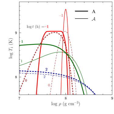
Figure 2: Excess temperature profiles versus density at four moments of time $t$=0.1, 1, 10 and 100 h (marked by $\log t$ [h]) after an instant toy burst ${\cal A}$ in the thin shell at $\rho=10^{8}$ g cm^-3 with the total energy release $E_{0}=9.08\times 10^{39}$ erg (thin lines). Thick lines are the same but produced by toy burst A from the shell of finite thickness. See the text for details.

The excess temperature profiles $T_{1}(\rho)$ are given by equation (10). Fig. 2 shows these profiles (thin lines) produced in the outer crust of the neutron star after burst ${\cal A}$ in an ignition shell with the total energy release $H_{0}=9.08\times 10^{39}$ erg; $T_{1}$ is plotted as a function of density at four moments of time $t$ since the burst starts, $t$= 0.1, 1, 10 and 100 hours. Thick lines show similar profiles for burst A in the shell of finite thickness.

An initial delta-function temperature spike becomes lower, wider and asymmetric and then disappears as the heat spreads over the crust. In this model, stage I lasts for about 10 h during which the thermal wave moves predominantly to the surface and reaches the outer layers ($\rho\sim 10^{7}$ g cm^-3). Stage II lasts till $t\sim(30-40)$ h. By this time the $T_{1}(\rho)$ profile becomes nearly horizontal above the ignited shell. Heat diffusion slows down, which suppresses the heat flow to the surface. At the last stage III the internal thermal wave moves slowly inside the star beyond the ignition shell.

The appropriate lightcurve for burst ${\cal A}$ is plotted in Fig. 3 along with the lightcurves for other burst models. The lightcurve reaches its peak in $t\approx 20$ hours when the most energetic part of the thermal wave emerges at the surface. Later the lightcurve decays; the decay is nearly power-law at the final stage.

Figure 3: Thick lines show burst luminosity versus time for toy-burst models A and B (Table 1) assuming $T_{0}\to 0$. The segments of especially high $L(t)$ are not shown because the toy-model cannot reproduce them accurately. Dashed lines are the lightcurves for the associated models ${\cal A}$ and ${\cal B}$ of instant bursts in the ignition shell ($\rho=\rho_{2}$). See the text for details.

Actually, the temperature profiles $T_{1}(\rho)$ at the early stages of the instant ignition-shell burst models contain rapidly increasing segments which are unstable against convection. The convection can change the temperature profiles and the early segments of lightcurves, which we discuss below for more realistic burst model A.

3.2 Basic properties of instant bursts

Equation (10) possesses the following properties.

Firstly, in a small vicinity near the heater ($|z-z_{\text{h}}|\ll z_{\text{h}}$) just after the heat release equation (10) reduces to

$$T_{1}(z,t)=\frac{H_{0}}{2C_{\text{h}}\sqrt{\pi\mathcal{D}_{\text{h}}t}}\exp\left(-\frac{(z-z_{\text{h}})^{2}}{4\mathcal{D}_{\text{h}}t}\right).$$ (14)

where $\mathcal{D}_{\text{h}}=b/(az_{\text{h}})$ and $C_{\text{h}}=az_{\text{h}}^{3}$ have meaning of the diffusion coefficient and the heat capacity near the heater, respectively. This is the well known temperature distribution produced after a point-like and instant heat release in a uniform medium. Accordingly, just after the burst one half of the thermal energy diffuses to $z\to 0$ while the other half diffuses to $z\to\infty$.

Secondly, it is easy to show that if a neutron star crust consisted solely of the toy-model matter down to the surface $z=0$, all the heat generated within the crust would diffuse, on a long run, within the star. No heat would be able to flow through the surface because the toy thermal conductivity (6) vanishes at $z=0$. The initial heat outflow to the surface would be redirected later inside the star (Fig. 2). This is the basic heat-accumulating property of inner layers of the outer neutron star crust. This possibility of heat accumulation in the crust has been pointed out by Eichler & Cheng (1989). Since the heat diffusion problem is linear in the toy model, the heat propagation from extended heaters would possess the same property.

The heat diffusion described formally by equation (10) to $z=0$ would give finite $T_{1}(t)$ but zero heat flux at $z=0$. This excess temperature $T_{1}(t)$ would grow up when the thermal wave reaches the surface; it would fall down later when the heat would start sinking inside the star after reflecting off the absolutely insulating surface.

This unphysical behaviour is caused by the formal extension of the toy model to $z\to 0$, discussed in the Appendix. Actually, the physical assumptions underlying the toy model are only justified in the $\rho-T$ domain (1). Therefore, in the figures we only show the results obtained using the toy model at $\rho>10^{7}$ g cm^-3. Microphysics in the outer layer ($\rho\lesssim 10^{7}$ g cm^-3) is different and allows some heat to outflow through the surface, which we approximately describe by introducing the heat blanketing envelope (Section 2.4).

Even in the selected domain (1) the toy model may somewhat exaggerate the announced heat accumulation (due to the neglect of quantum suppression of heat capacity of crystalline ions) or to underestimate it (because of the neglect of the electron contribution to the heat capacity). Nonetheless, we believe (and confirm by the numerical simulations) that the model adequately reflects this heat accumulation and enables one to study its consequences.

Note that at $t\gg(u^{2}+u_{\text{h}}^{2})/4$ from equation (10) we have

$$T_{1}(z,t) = \frac{H_{0}}{3b\sqrt{z_{\text{h}}z}\,t\,\Gamma(4/3)}\,\left(\frac{u_{\text{h}}u}{4t}\right)^{1/3}$$ (15)

$$= \frac{H_{0}}{3b\Gamma(4/3)}\left(\frac{a}{9b}\right)^{1/3}\frac{1}{t^{4/3}},$$

where $\Gamma(4/3)\approx 0.893$ is the gamma-function value. In this case, $T_{1}(z,t)$ becomes independent of $z$ and $z_{\text{h}}$ and decreases with $t$ as $t^{-4/3}$, determining the very late asymptotic behaviour of the lightcurve $L(t)$.

4 Finite-width shell burst A

4.1 Overview

Here we discuss burst A (Table 1) in a sufficiently thick spherical layer [$\rho=(3-10)\times 10^{7}$ g cm^-3] that fully lies within the toy-model density range (1). Model ${\cal A}$, that has been analysed in Section 3, represents a thin-shell counterpart of model A.

The thick lines in Fig. 2 show snapshots of the toy-model A excess temperature profiles $T_{1}$ versus $\rho$ at different moments of time in comparison with burst ${\cal A}$ (thin lines). The $T_{1}(\rho)$ curves can be regarded as the $T(\rho)$ curves in the $T_{0}\to 0$ approximation. We see that the A and ${\cal A}$ profiles of $T_{1}(\rho)$ in Fig. 2 are different at $t\lesssim 1$ d. The largest difference is just after the burst (with flat $T_{\text{f}}(\rho)$-profile within the heater for burst A versus sharp spike for burst ${\cal A}$) but they become close later. The appropriate lightcurves can be compared in Fig. 3 with the same conclusion.

We have checked that the internal temperature profiles and lightcurves at the late stage III (Section 2.7) of burst model B (Table 1) are well described by the respective model ${\cal B}$. This seems to be a generic feature of bursts associated with the fact that the main burst energy is released near the ignition density $\rho_{2}$.

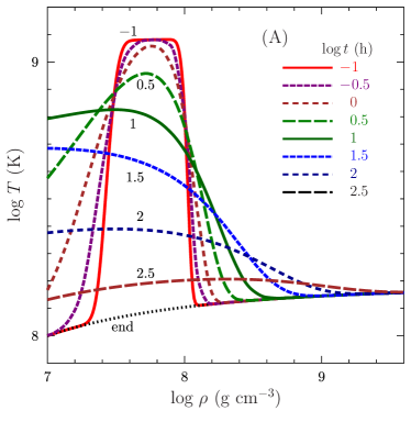
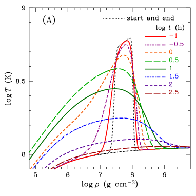
Figure 4: Density dependence of the internal temperature $T(\rho)$ in the outer neutron star crust after burst A at different moments of time $t$ (marked by $\log t$ [h]) assuming $T_{\text{b0}}=10^{8}$ K at $\rho=10^{7}$ g cm^-3 prior to the burst. The curves on the left-hand panel are calculated with the toy model, while those on the right-hand panel are computed with the numerical code that allows us to extend them to lower $\rho$. The lower dotted curves on both panels are pre-burst (= after-burst) temperatures $T_{0}(\rho)$. See the text for details.

Fig. 4 presents the internal temperature profiles $T(\rho)$ at different moments of time $t$ (marked by the values of $\log t$ [h]) after burst A assuming the pre-burst temperature $T_{\text{b0}}=10^{8}$ K at $\rho=10^{7}$ g cm^-3. The curves on the left-hand panel are calculated using the toy model while the curves on the right-hand panel are calculated by the thermal evolution code. The lower dotted line is the temperature profile $T_{0}(\rho)$ without any burst [it is given by equation (9) for the toy model]. As explained in Section 2.5, the code allows us to compute the $T(\rho)$ profiles at any densities. Here the outer envelope with mass $M_{\text{env}}=10^{-14}\,\mbox{$\textrm{M}_{\odot}$}$ is used, which enables us to display the $T(\rho)$ curves to lower densities $\rho\sim 10^{5}$ g cm^-3 in the right-hand panel.

Fig. 5 presents the lightcurves for burst A calculated using the toy model (on the left-hand panel) and the thermal evolution code (on the right-hand panel). The solid curve in the left-hand panel and both curves in the right-hand one refer to $T_{\text{b0}}=10^{8}$ K at $\rho=10^{7}$ g cm^-3; the corresponding levels of the quiescent thermal luminosity of the star are plotted by the horizontal dotted lines. The dashed line for the toy model presents the lightcurve assuming $T_{0}\to 0$ (as in Fig. 3). The solid and dashed lines on the right-hand panel are computed for the same burst model but using different heat blankets (with equivalent $\rho_{\text{b}}=5\times 10^{4}$ and $10^{5}$ g cm^-3, respectively). The nice agreement between these curves shows that the outer quasi-stationary envelope of $M_{\text{env}}=10^{-14}\,\mbox{$\textrm{M}_{\odot}$}$ is sufficiently thin to ensure good accuracy of the simulations.

According to Fig. 3, burst A becomes pronounced in the surface emission in a few hours after the explosion, in contrast with $\sim 10$ hours for burst ${\cal A}$. This is because the outer part of the burning layer A is closer to the surface.

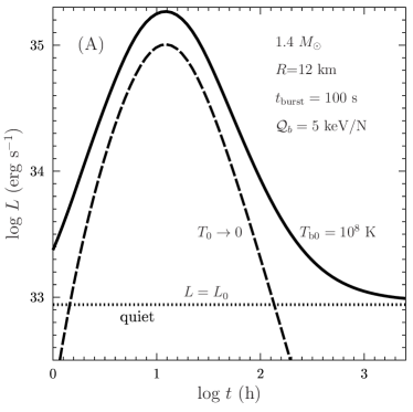
Figure 5: Surface luminosity versus time for burst A calculated with the toy model (left) and with the thermal evolution code (right). The solid line on the left-hand panel as well as solid and dashed lines on the right-hand panel correspond to $T_{\text{b0}}=10^{8}$ K at $\rho=10^{7}$ g cm^-3 prior to the burst; the horizontal dotted lines display the quiescent luminosity. The dashed line on the left-hand panel shows the toy lightcurve assuming $T_{0}\to 0$ (as in Fig. 3). The solid and dashed lines on the right-hand panel are computed with different heat blanket models. The vertical dotted line in the right-hand panel is a guide to the eye for comparison with the solid line in the left-hand panel. See text for details.

4.2 Burst A: toy model versus simulations

Now we can compare the toy-model results with those provided by the numerical simulations. Figs. 4 and 5 allow us to compare $T(\rho)$ profiles and the lightcurves of burst A.

The overall qualitative agreement seems reasonable although some differences are substantial. The differences are visible at stage I which lasts for a few hours and at stage II, that ends in about 30 hours. The agreement between the toy and accurate results at the last decay stage III is more satisfactory.

The main source of disagreement is in the underestimation of the heat capacity at $\rho\sim 10^{7}$ g cm^-3 in the toy model (as discussed above; Fig. 1) and much more realistic treatment of the heat transport to the very surface by the numerical code. With the reduced toy heat capacity, the instant-afterburst toy temperature $T_{\text{f}}(\rho)$ (Section 2.6) in the burning zone becomes higher than it should be. These instant afterburst segments of the $T_{\text{f}}(\rho)$ curves are quite visible in Fig. 4 (at $\log t\ [{\rm h}]=-1$ and $-0.5$). The largest $T_{\text{f}}$ difference reaches a factor $\sim(2-3)$ at $\rho=3\times 10^{7}$ g cm^-3. As a result, the toy model overheats the matter at lower densities, making the lightcurve noticeably brighter than it should be at stages I and II. It overestimates the burst energy radiated at these stages through the surface and reduces in this way heat-accumulating properties of neutron stars. Owing to these reasons we do not show most luminous segments of the toy lightcurve B in Fig. 3. According to the simulations, about 20 per cent of the burst energy emerges through the surface in burst A. The toy model does not allow us to accurately estimate this value.

Let us note sufficiently large temperature gradients of the toy $T(\rho)$ profiles (Fig. 4) near $\rho_{\text{b}}=10^{7}$ g cm^-3 at stage I. They are expected to be badly compatible with the toy heat blanket model (Section 2.4) making the toy lightcurve even less reliable. Note also that the quiescent (dotted) $T(\rho)$ profile is steeper for the toy model.

On stages II and III, both approaches predict nearly horizontal segments of the $T(\rho)$ profiles (with small inclinations relative to the horizontal axis) which correspond to quasi-stationary and nearly flux-conserving heat propagation. These segments appear rather insensitive to microphysics of the matter: the heat capacity drops out of equation (3) in the stationary case and the thermal conductivity should only be high enough to ensure almost horizontal profiles.

4.3 Convection after burst A

Steeply rising segments of the $T(\rho)$ profiles for bursts A and ${\cal A}$ at stage I in Figs. 2 and 4 can be convectively unstable. The convection has been neglected both in the toy model and in the numerical simulations. Let us outline it for the toy model after burst A. To estimate the deepest densities of the convective zone, we have used accurate microphysics of fully ionized plasma of iron matter. We have employed the Schwarzschild convection criterion and compared the toy-model temperature gradients with the adiabatic ones.

As a result, we have obtained that the convection can operate at stage I for about 5 hours after the burst. Later the bottom density of the convective zone becomes lower than $\rho_{\text{b}}=10^{7}$ g cm^-3, and the convection disappears from the toy-model domain (1). It can still operate at $\rho<\rho_{\text{b}}$, but it cannot strongly affect the model lightcurves and heat propagation at $\rho>\rho_{\text{b}}$.

If the convection is on, the real $T(\rho)$ profiles lie between the heat-diffusion and adiabatic temperature profiles, and the latter can be essentially higher than the former. We do not plot the adiabatic $T(\rho)$ curves and we do not follow the consequences of convection in detail because we regard models A and ${\cal A}$ as illustrative.

5 Thick-shell burst B

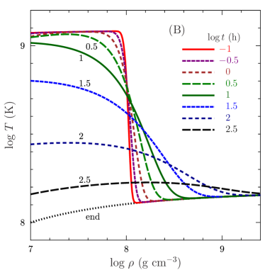
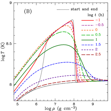
Figure 6: Same as in Fig. 4 but for burst B.

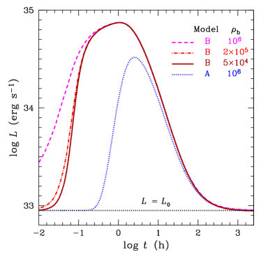
Figure 7: Surface luminosity versus time for bursts from the four shells extended from $\rho_{\text{b}}$ to $10^{8}$ g cm^-3 (see the legend), computed assuming a quasi-stationary outer envelopes of masses $M_{\text{env}}=(10^{-12}$, $10^{-13}$, $10^{-14})$ $\textrm{M}_{\odot}$, corresponding to the $T$-dependent bottom densities $\rho_{\text{b}}(T)$, whose approximate values $\sim(10^{6}$, $2\times 10^{5}$, 5$\times 10^{4}$) g cm^-3 are marked in the legend. The dotted line for burst A (Fig. 5) is shown for comparison with the other lines, which are computed for model B. The lower horizontal dotted line is the quiescent luminosity (with $T_{\text{0}}=10^{8}$ K at $\rho=10^{7}$ g cm^-3). See the text for details.

Fig. 6 shows snapshots of the temperature profiles $T(\rho)$ in the outer crust of the star after burst B (Table 1) at different moments of time $t$. The curves are calculated using the toy model (the left-hand panel) and the thermal evolution code (the right-hand panel) under the assumption that $T=10^{8}$ K at $\rho=10^{7}$ g cm^-3 prior to the burst. Fig. 6 is analogous to Fig. 4 for burst A. As in Fig. 4, the temperature profiles are traced to lower $\rho$ in the right-hand panel.

Burst B is designed to be a more adequate representation of a realistic superburst than burst A. Let us recall that the toy model is justified at $\rho>\rho_{\text{b}}=10^{7}$ g cm^-3, while it is widely accepted that explosive carbon burning in superbursts occurs also at much lower densities, down to $\rho_{1}\sim 10^{4}$ g cm^-3 or lower (e.g. Keek & Heger 2011; Keek et al. 2012). However, the main energy release takes place at $\rho\gtrsim\rho_{\text{b}}$ so that the burning at lower densities does not change the total energy budget, although it affects the temperature distribution at $\rho\lesssim\rho_{\text{b}}$, including densities somewhat higher than $\rho_{\text{b}}$.

To be consistent with standard simulations of superbursts, in the toy model B we use the solution of equation (12), in which the heat source is extended to lower densities $\rho_{1}$, as in real superbursts. We have taken $\rho_{1}=3\times 10^{6}$ g cm^-3; making $\rho_{1}$ still lower would not change our results. This choice of the toy-model solution gives realistic behaviour of the temperature distribution $T(z,t)$ in the toy-model domain (1). However, some extra energy is now released in the density range $\rho<10^{7}$ g cm^-3, where we use the heat-blanket solution to calculate the lightcurve. The heat-blanket model is obtained without any additional short-term heating. Accordingly, we cannot rely on our lightcurve as long as the extra heat is confined in the heat blanket and the usual steady-state heat outflow is not established there.

Using the above procedure, we obtain the toy-model $T(\rho)$ profiles at $\rho\geq 10^{7}$ g cm^-3  (the left-hand panel of Fig. 6) which are stable against convection and resemble those obtained in advanced simulations of superbursts.

The main difference of these profiles from those for toy burst A on the left-hand side of Fig. 4 is the absence of temperature peaks associated with the finite width of the heater A. The toy-model temperature gradient for burst B is mainly negative at $\rho\geq\rho_{\text{b}}=10^{7}$ g cm^-3 at all moments of time because of the heat-accumulation nature of the toy model. In the density range $\rho_{\text{b}}\leq\rho\lesssim\rho_{2}$, this gradient decreases with time, leading to the appearance of quasi-isothermal zones (in $t\approx$ 30 h for burst B). The extra heat accumulated in this zone mainly sinks slowly inward the star in the same manner as in burst A.

The calculated toy-model temperature profiles are in reasonable qualitative agreement with those computed using the thermal evolution code and presented on the right-hand panel of Fig. 6 (as in Section 4 for burst A). However, the toy model stronger overestimates $T$ at $\rho\sim 10^{7}$ g cm^-3 at earlier stages I and II, although the overall agreement at the late stage III is satisfactory. The slower toy-model thermal diffusion is also quite visible. Apparently faster cooling of the heated layer in the numerical calculations is realized because of stronger heat outflow through the surface. As explained above, the extra energy, generated at $\rho<\rho_{\text{b}}$, complicates construction of the toy-model lightcurve at the initial stages I and II of burst B, although the agreement improves with time and becomes better at stage III.

In Fig. 7 we present three lightcurves calculated by the numerical code for burst B model ($\rho_{1}=3\times 10^{6}$ g cm^-3) compared with one lightcurve for burst A ($\rho_{1}=3\times 10^{7}$ g cm^-3). The former three curves differ by the masses $M_{\text{env}}$ of the quasi-stationary envelope used in simulations. We parametrize these masses by the approximate equivalent values of $\rho_{\text{b}}$ listed in Section 2.5. Although the lightcurves for burst B are somewhat different at stage I ($t\lesssim 10$ min), they merge in the single curve later. At stage III ($t\gtrsim 20$ h) this curve is similar but slightly higher than the dotted curve for burst A, because burst B is more energetic (Table 1). This similarity is a genetic feature of lightcurves at stage III, as discussed below. Very similar behaviour is due to the same bottom density $\rho_{2}$ of the bursting shells in models B and A. According to the numerical simulations, about 25 per cent of the energy released in burst B emerges through the surface. It is higher than 20 per cent in burst A, because model B contains heating layers located closer to the surface.

6 Generic features of bursts

Let us outline generic features of the stages I, II and III in the evolution of deep bursts (Section 2.7).

Stage I is short and dynamical. It can be accompanied or not accompanied by convection, depending of the fuel distribution in the burning shell. For realistic bursts of thick shells filled with fuel to low densities ($\lesssim 10^{4}$ g cm^-3), convection seems unimportant (because of reduction of temperature gradients). Stage I ends with the onset of quasi-stationary flux-conserving heat outflow at $\rho\sim(10^{6}-10^{7})$ g cm^-3.

The next stage II of the strongest energy release through the surface is accompanied by quasi-equilibration of the heat propagation though the entire bursting shell (down to the ignition depth $\rho_{2}$). According to many simulations (e.g. Cumming & Macbeth 2004; Cumming et al. 2006; Altamirano et al. 2012), the lightcurves $L(t)$ show a rapid initial rise (not always observable) followed by a slow, e.g. power-law fall; the power-law index is often treated as universal. Typically, the initial afterburst temperature profiles $T_{\text{f}}(\rho)$ gradually increase with density. However, as demonstrated by Keek et al. (2015), one can obtain steeper profiles, for instance assuming that the fraction of burnt fuel increases with $\rho$ within the heated layer. In this case, the authors obtained the $L(t)$ curves containing smooth peaks at the most energetic stage. Lightcurves of both types, with a slow $L(t)$ fall and with a preceding peak, have been observed.

We remark that microphysics in bursting sources can be different, for example due to different ignition densities and temperatures (see Section 7.2). Accordingly, we do not expect that the $L(t)$-profile at burst stage II is universal. Varying microphysics and the fuel distribution, one can construct rather sophisticated profiles.

By the end of the most energetic burst stage II, the quasi-stationary regime of flux-conserving heat outflow (e.g. Cumming et al. 2006) is established from the outer zone to the bottom of the initially heated layer, $\rho_{1}\leq\rho\lesssim\rho_{2}$.

Recall that the temperature becomes almost independent of heat capacity and thermal conductivity in nearly isothermal zones. Once such zones appear, calculated values of $T$ within them start to be insensitive to the underlying microphysics.

Before the temperature equilibrates in the entire heated zone during stage II, the heat has not enough time to sink deeply inside the crust. The latter sinking mainly proceeds at the final stage III of the burst.

7 Late stage of burst decay

Here we focus on stage III of late burst decay. So far our consideration was restricted to one neutron star model ($M=1.4\,\mbox{$\textrm{M}_{\odot}$}$, $R=12$ km) and to fixed ignition density ($\rho_{2}=10^{8}$ g cm^-3). We also restricted ourselves to unrealistically low fuel calorimetry, in order to meet the assumptions inherent to the toy model (in particular, the neglect of neutrino emission). In this section we will base on generic properties of bursts (Section 6) and perform a semi-quantitative analysis of the late decay stage III for rather arbitrary neutron star models, ignition depths, and burst energies. Our consideration will also be independent of possible strong neutrino cooling of the bursting shell at earlier stages I and II. The analysis will be not too rigorous but hopefully reproduces the main features of stage III under the assumption that the internal temperature is much higher than in quiescence, $T\gg T_{0}$.

7.1 Transition time to the late-decay stage

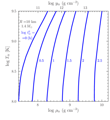
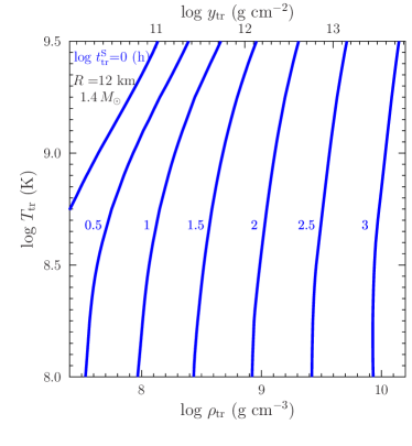
Figure 8: Isolines of constant thermal diffusion times ($\log t^{\text{S}}_{\text{tr}}{\rm[h]}=$0, 0.5, 1, 1.5, 2, 2.5 and 3) in the $\log\rho_{\text{tr}}-\log T_{\text{tr}}$ plane for neutron stars with $M=$1.4 $\textrm{M}_{\odot}$ and two values of $R$=10 km (left-hand panel) and 12 km (right-hand panel). Upper horizontal scales show column densities $y_{\text{tr}}$ (instead of $\rho_{\text{tr}}$) as commonly used in the literature. See the text for details.

The transition from the most energetic stage II to the final stage III can be observable as a transition to faster lightcurve decay. Let $t_{\text{tr}}$ be the corresponding transition time and $T_{\text{tr}}$ be the temperature in the nearly isothermal zone at this epoch. It is natural to state (e.g. Cumming & Macbeth 2004; Cumming et al. 2006; Altamirano et al. 2012) that $t_{\text{tr}}$ is the time of thermal wave propagation from the bottom of the heater through the entire outer zone (from the ignition density $\rho_{2}\approx\rho_{\text{tr}}$ to the surface). This time can be estimated as (Henyey & L’Ecuyer, 1969)

$$t_{\text{tr}}=\frac{1}{4}\,\left|\int_{0}^{z_{2}}{\rm d}z\,\sqrt{\frac{C}{\kappa}}\,\right|^{2},$$ (16)

where the integration is along the $T(z)$ track at $t\sim t_{\text{tr}}$. For deep and strong bursts, the internal temperature by that time becomes nearly uniform, $T\approx T_{\text{tr}}$, over the most important part of the track which contributes mainly to the integral.

In the toy model, it is sufficient to replace the lower integration limit by $z_{\text{b}}$ (that is appropriate to $\rho_{\text{b}}=10^{7}$ g cm^-3). Using equations (4) and (6), we obtain

$$t_{\text{tr}}=\frac{a}{{9}\ b}\,(z_{2}^{3/2}-z_{\text{b}}^{3/2})^{2}\approx\frac{a}{{9}\ b}\,z_{2}^{3}\approx{0.35}\,\rho_{\text{tr6}}\leavevmode\nobreak\ {\rm h};$$ (17)

the final expression is obtained by setting $z_{\text{2}}\gg z_{\text{b}}$, and the estimate is given for $M=1.4$ $\textrm{M}_{\odot}$ and $R=12$ km, with $\rho_{\text{tr6}}=\rho_{\text{tr}}/10^{6}$ g cm^-3. This gives $t_{\text{tr}}\approx 35$ h for toy bursts A and B.

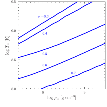
Figure 9: Isolines of constant power-law indices in equation (23), $\nu=$0.3, 0.4, 0.5, 0.6 and 0.7, on the $\log\rho_{\text{tr}}-\log T_{\text{tr}}$ plane for neutron stars (independent of $M$ and $R$). See the text for details.

Disregarding the toy model, we have calculated $t_{\text{tr}}$ from equation (16) along the $T=T_{\text{tr}}$ tracks for a dense grid of $\log\rho_{\text{tr}}\leavevmode\nobreak\ [\mbox{g\leavevmode\nobreak\ cm${}^{-3}$}]$ (from 7.5 to 10 with step of 0.1) and $\log T_{\text{tr}}\leavevmode\nobreak\ [{\rm K}]$ (from 8 to 9.5 with step of 0.1). We have taken the lower integration limit at $\rho=10^{6}$ g cm^-3  and used full realistic physics input. The calculated values present realistic estimates of thermal diffusion time from depths $\rho_{\text{tr}}$ at temperatures $T_{\text{tr}}$ to the surface. The entire family of these diffusion times can be fitted by

$$t^{(0)}_{\text{tr}}[{\rm h}]=p_{1}\rho_{\text{tr6}}^{p_{3}+1}/(1+p_{2}\rho_{\text{tr6}}^{p_{3}}),$$ (18)

where

$$p_{1} = \frac{0.07483(l_{T}-7.786)}{1+\exp(11.37(l_{T}-8.576))}+3\times 10^{-5},$$

$$p_{2} = \frac{0.5582(l_{T}-7.777)}{1+\exp(10.87(l_{T}-8.587))}+3.9\times 10^{-4},$$

$$p_{3} = 0.8209+0.3865\,\sin(3.658(l_{T}-14.04)),$$

and $l_{T}=\log_{10}(T_{\text{tr}}\leavevmode\nobreak\ [\rm K])$. The maximum relative fit error is about 9 per cent (at $\log\rho_{\text{tr}}[\mbox{g\leavevmode\nobreak\ cm${}^{-3}$}]=7.5$ and $\log T_{\text{tr}}[{\rm K}]=8$) and the rms relative error is 3 per cent, quite sufficient for our semi-quantitative analysis. The superscript $(0)$ in $t^{(0)}_{\text{tr}}$ indicates that the calculated values refer to a star with $M=1.4$ $\textrm{M}_{\odot}$, $R=12$ km and $g_{\text{s0}}=1.59\times 10^{14}$ cm s^-2.

Note that we determine $t_{\text{tr}}$ in the local reference frame. According to equation (13) and simple self-similarity arguments, a distant observer would measure

$$t^{\text{S}}_{\text{tr}}=\,\frac{g_{\text{s0}}^{2}}{g_{\text{s}}^{2}}\,\frac{t_{\text{tr}}^{(0)}}{\sqrt{1-r_{\text{g}}/R}}$$ (19)

for a neutron star with arbitrary values of $M$ and $R$ (and corresponding surface gravity $g_{\text{s}}$).

For example, Fig. 8 shows the isolines of constant $\log t_{\text{tr}}[{\rm h}]$=0.5, 1, 1.5 and 2 in the $\rho_{\text{tr}}-T_{\text{tr}}$ plane for neutron stars with the canonical mass $M=1.4$ $\textrm{M}_{\odot}$ but two values of radius $R=10$ km (the left-hand panel) and $R=12$ km (the right-hand panel). It is seen that $t_{\text{tr}}$ depends mainly on $\rho_{\text{tr}}$. For the same $\rho_{\text{tr}}$, the diffusion time is noticeably shorter in a more compact star because its crust is geometrically thinner. In the toy model, the diffusion time (17) appears somewhat larger because our toy-model thermal conduction is slower.

Inferring $t_{\text{tr}}$ from observations allows one to estimate the ignition depth $\rho_{\text{tr}}$ (or ignition column $y_{\text{tr}}$) and put constraints on possible mass and radius of the star. At $t\sim t_{\text{tr}}$ one expects $T_{\text{tr}}\sim(1-3)\times 10^{9}$ K and the luminosity of a real superburst $L_{\text{tr}}\sim(5-50)\times 10^{35}$ erg s^-1.

7.2 Late decay rate

Here we analyse the burst decay rate at $t\gtrsim t_{\text{tr}}$.

First of all we note that the transition temperature $T_{\text{tr}}$ can roughly be estimated as the temperature of the outer layer $\rho_{\text{min}}\lesssim\rho\lesssim\rho_{2}$ heated by the nuclear column energy (that is, the energy per unit surface area), $H_{\text{0tr}}$, released in the outer layer by the moment $t\sim t_{\text{tr}}$. Generally, the initial heat $H_{0}$ can be transported outward (to the surface), inward (to the core) and carried away by neutrinos from the heated layer. The inward heat transport is slow; it can usually be ignored at $t\lesssim t_{\text{tr}}$. The heat transport to the surface can be efficient at $t\lesssim t_{\text{tr}}$ but later it becomes less important compared with the inward heat flux. The neutrino emission (which we ignore in the bulk of this paper) can substantially reduce the thermal energy but this energy loss is quick (because it is the strongly $T$-dependent, see Yakovlev et al. 2001). It is expected to become weak at $t\gtrsim t_{\text{tr}}$. Thus we can estimate $T_{\text{tr}}$ as

$$T_{\text{tr}}\sim H_{\text{0tr}}/(C_{\text{tr}}z_{\text{tr}}),$$ (20)

where $C_{\text{tr}}=C(z_{\text{tr}},T_{\text{tr}})$.

The last stage of the burst decay is controlled by sinking of the heat inside the star. The heat capacity of the outer crust under the heater is so large that the matter easily absorbs the spreading heat. Accordingly, in spite of high thermal conductivity, the heat wave moves slowly inside the star, increasing heat-accumulating property of the outer crust.

This slow heat sinking is governed by equation (3) with $Q=0$. At $t\gtrsim t_{\text{tr}}$ an approximate solution can be obtained using self-similarity properties inherent to this equation. Let $z_{*}$, $T_{*}$, $C_{*}$ and $\kappa_{*}$ be, respectively, characteristic depth, excess temperature, heat capacity and thermal conductivity of the inner front ($z_{*}\gtrsim z_{\text{tr}}$) of the spreading heat at moment $t$. At $t\gtrsim t_{\text{tr}}$ one can use the following order-of-magnitude estimates,

$$T_{*}C_{*}z_{*}\sim H_{\text{0tr}},\quad t\sim C_{*}z_{*}^{2}/\kappa_{*}.$$ (21)

The first estimate ensures approximate conservation of the overall heat content over time, in agreement with equation (20), and the second one describes ordinary heat diffusion.

Now let us assume arbitrary power-law dependences of $C$ and $\kappa$ on temperature and density

$$C(z,T) = C_{\text{tr}}\left(\frac{z}{z_{\text{tr}}}\right)^{\alpha_{1}}\left(\frac{T}{T_{\text{tr}}}\right)^{\alpha_{2}},$$ (22a)

$$\kappa(z,T) = \kappa_{\text{tr}}\left(\frac{z}{z_{\text{tr}}}\right)^{\beta_{1}}\left(\frac{T}{T_{\text{tr}}}\right)^{\beta_{2}},$$ (22b)

and analyse the thermal wave propagation recalling that $\rho\propto z^{3}$, in deep layers of the outer crust. Here, $C_{\text{tr}}$ and $\kappa_{\text{tr}}$ normalize the heat capacity and thermal conductivity, while $\alpha_{1}$, $\alpha_{2}$, $\beta_{1}$ and $\beta_{2}$ specify their density and temperature dependence. For a normalization point, we take $z=z_{\text{tr}}$ at the moment $t=t_{\text{tr}}$ at which the late afterburst relaxation stage III starts, with $T_{*}=T_{\text{tr}}$. We substitute equations (22) into (21) and obtain two equations containing powers of $t/t_{\text{tr}}$, $z_{*}/z_{\text{tr}}$ and $T_{*}/T_{\text{tr}}$. These equations yield the self-similar solution for arbitrary microphysics of the matter in the form of power-law decay,

$$\frac{T_{*}}{T_{\text{tr}}}\sim\left(\frac{t_{\text{tr}}}{t}\right)^{\nu}\sim\left(\frac{z_{\text{tr}}}{z_{*}}\right)^{(\alpha_{1}+1)/(\alpha_{2}+1)},$$ (23)

where the power index is

$$\nu=\frac{1+\alpha_{1}}{2+\alpha_{1}+\alpha_{2}+(1+\alpha_{1})\beta_{2}-(1+\alpha_{2})\beta_{1}}.$$ (24)

The toy model corresponds to $\alpha_{1}=3$, $\beta_{1}=2$, $\alpha_{2}=\beta_{2}=0$ and gives $\nu=4/3$. At $H_{\text{0tr}}\sim H_{0}$ equation (23) qualitatively reproduces the exact asymptotic solution (15) of the toy model problem for the internal temperature decay and yields the law of thermal wave propagation inside the star, $\rho_{*}/\rho_{\text{tr}}\sim(z_{*}/z_{\text{tr}})^{3}\sim t/t_{\text{tr}}$, which agrees with the toy model calculations. However, let us stress that, for the parameters employed, the exact toy asymptotic regime is realized too late to be observed in real events.

Nevertheless, the real plasma deviates from the toy-model due to the complexity of microphysics involved (Section 2.1). We see that the index $\nu$ reflects the rate of temperature decrease in the vicinity of the depth $z_{\text{tr}}$ at the moment of time $t_{\text{tr}}$. This $\nu$ is local (depends on local density $\rho_{\text{tr}}$ and temperature $T_{\text{tr}}$), but independent of neutron star mass and radius. For any pair of $\rho_{\text{tr}}$ and $T_{\text{tr}}$ we have calculated the parameters $\alpha_{1,2}$ and $\beta_{1,2}$ in equation (22) as local power-laws, e.g., $\alpha_{1}=\partial\ln C(z,T)/\partial\ln z$ (at $z=z_{\text{tr}}$ and $T=T_{\text{tr}}$) with accurate microphysics of the matter. Then we have found $\nu$ from equation (24). Fig. 9 presents isolines of constant $\nu$=0.3, 0.4, 0.5, 0.6 and 0.7 in the $\rho_{\text{tr}}-T_{\text{tr}}$ plane. One can see that higher $\nu$ are realized at sufficiently large densities and low temperatures.

Indeed, the microphysics of the matter varies with density and temperature. For instance, at densities $\rho\sim 10^{7}$ g cm^-3 the approximation of temperature-independent thermal conductivity of degenerate electrons (6) is violated, and the linear dependence $\kappa\propto T$ becomes more suitable (e.g. Potekhin et al. 1999). Then, as long as the degenerate electrons remain relativistic, one has $\kappa\propto T\rho^{1/3}$, which corresponds to $\beta_{1}=\beta_{2}\approx 1$. As for the heat capacity, it may still be mostly provided by ions, with $C\propto\rho$ ($\alpha_{1}=3$, $\alpha_{2}=0$), as in the toy model; see equation (4). In that case, we have $\nu=1/2$, so that $T_{*}/T_{\text{tr}}\sim\sqrt{t_{\text{tr}}/t}$ and $\rho_{*}/\rho_{\text{tr}}\sim(t/t_{\text{tr}})^{3/8}$. Note that Cumming & Macbeth (2004) obtained $\nu=2/3$ which is largely used in the literature. Fig. 9 demonstrates that a wide range of $\nu$ can be realized in one star.

Now we can outline the behaviour of the lightcurve $L(t)$ at the decay stage III. To this aim, we can assume that at $t\gtrsim t_{\text{tr}}$ the internal temperature profile at densities $\rho_{\text{b}}\lesssim\rho\lesssim\rho_{*}$ is nearly flat, $T(\rho)\approx T_{*}$. Then we can estimate the surface temperature $T_{\text{s}}$ and the surface luminosity $L(t)=4\pi R^{2}\sigma_{\text{SB}}T_{\text{s}}^{4}$ with the aid of the $T_{\text{s}}-T_{\text{b}}$ relation for the heat blanketing envelope (Section 2.4). These results can be roughly approximated by the power-law decay

$$L(t)\approx(t_{\text{tr}}/t)^{\gamma}\,L_{\text{tr}},$$ (25)

with the index $\gamma={\rm d}\ln L(t)/{\rm d}\ln t$ at $t=t_{\text{tr}}$. Unfortunately, our calculations show that accurate values of $\gamma$ do depend on deviations of $T(\rho)$ from constants $T_{\text{tr}}$ near the heat blanket ($\rho>10^{7}$ g cm^-3) and on exact behaviour of the $T_{\text{s}}-T_{\text{b}}$ relation at $\rho=\rho_{\text{b}}$. The problem of accurate calculation of $\gamma$ deserves a special study. The robust conclusion is that $\gamma$ is larger for deeper bursts (higher $\rho_{\text{tr}}$) and lower $T_{\text{tr}}$. These results do not support the idea that $\gamma$ is universal for all superbursts.

One should bear in mind that the self-similar approach is only an approximation based on the assumptions that local miscophysical parameters, such as $\alpha_{1,2}$ and $\beta_{1,2}$ vary sufficiently slowly. It is natural that as the crust is cooling at stage III, microphysics of the characteristic density and temperature domain, that controls the cooling, is changing. This may lead to a variable $\gamma$ along the cooling track.

7.3 Analysing late superburst tails

The results on times $t\gtrsim t_{\text{tr}}$ of late superburst decay onset (Section 7.1) and on lightcurve slope $\gamma$ during the late tail stage III (Section 7.2) can be used for a preliminary semi-quantitative ‘express’ analysis of superbursts. A transition time $t^{\text{S}}_{\text{tr}}$ from stage II to stage III can be observed as a change of the lightcurve slope (from a slow to faster decay). A power-law index $\gamma$ can potentially be inferred from an observed lightcurve at stage III. Note that both measurements (of $t^{\text{S}}_{\text{tr}}$ and $\gamma$) do not require normalization of lightcurves. It is worth to remark that the accurate determination of $\gamma$ is a serious problem because of large errorbars of $L(t)$ at the tail stage when the source is fading. Analysing $t_{\text{tr}}$ seems more informative.

For instance, let us consider six superbursts detected with BeppoSAX and analysed by Cumming et al. (2006). They were the superbursts from 4U 1524–690 observed in 1999 (in ’t Zand et al., 2003); 4U 1735–444 (1996, Cornelisse et al. 2000); KS 1731–260 (1996, Kuulkers et al. 2002); GX 17+2 (1999, in ’t Zand, Cornelisse & Cumming 2004), Ser X-1 (1997, Cornelisse et al. 2002); 4U 1636–536 (2001, Strohmayer & Markwardt 2002; Kuulkers et al. 2004). The observed lightcurves and theoretical fits are given in figs. 5–10 of Cumming et al. (2006); the fit parameters are listed in table 1 of that paper.

Let us take, for instance, the KS 1731–260 superburst (fig. 5) and determine $t_{\text{tr}}^{\text{S}}$ as the time after which the theoretical fit becomes nearly power-law. We have $t_{\text{tr}}^{\text{S}}\approx 10$ h. Since Cumming et al. (2006) took $M=1.4\,\mbox{$\textrm{M}_{\odot}$}$ and $R=10$ km for their interpretation, we use the left-hand panel of Fig. 8, adopt $\log T_{\text{tr}}$ [K]$\approx 9-9.3$ and obtain $\log y_{\text{tr}}\leavevmode\nobreak\ [{\rm g\leavevmode\nobreak\ cm^{-2}}]\approx 12$ and $\log\rho_{\text{tr}}[\mbox{g\leavevmode\nobreak\ cm${}^{-3}$}]\approx 8.7$, in nice agreement with Cumming et al. (2006). Similar agreement takes place for other five superbursts. Note, however, that in order to explain the reported $\log y_{\text{tr}}\leavevmode\nobreak\ [{\rm g\leavevmode\nobreak\ cm^{-2}}]\approx 11.7$ ($\log\rho_{\text{tr}}[\mbox{g\leavevmode\nobreak\ cm${}^{-3}$}]\approx 8.5$) for the shortest superburst ($t_{\text{tr}}^{\text{S}}\approx 2$ h), demonstrated by 4U 1636–536, we need to assume higher $\log T_{\text{tr}}\leavevmode\nobreak\ [{\rm K}]\approx 9.5$.

Now let us return to the KS 1731–260 superburst and take the same $M=1.4\,\mbox{$\textrm{M}_{\odot}$}$ but larger $R=12$ km. In this case, we should use the right-hand panel of Fig. 8. With the same $t_{\text{tr}}^{\text{S}}$ and $\log T_{\text{tr}}$ we obtain $\log y_{\text{tr}}[\mbox{g cm${}^{-2}$}]\approx 11.3$ and $\log\rho_{\text{tr}}[\mbox{g\leavevmode\nobreak\ cm${}^{-3}$}]\approx 8.2$. With the larger radius $R$, the crust becomes thicker, which makes thermal diffusion slower. Accordingly the ignition density $\rho_{\text{tr}}$ has to be about three times smaller to ensure the same time $t_{\text{tr}}^{\text{S}}$ for the late stage III onset. Similar shifts of the ignition density to the surface would take place for other superbursts, meaning that theoretical interpretation of superbursts is rather sensitive to neutron star mass and radius. Our Fig. 8 and equations (18) and (19) can be helpful for understanding which $M$ and $R$ are more suitable.

Let us mention again the remarkable superburst of 4U 1636–536 with $t_{\text{tr}}^{\text{S}}\approx 2$ h. Recall that Cumming et al. (2006) assumed $M=1.4\,\mbox{$\textrm{M}_{\odot}$}$ and $R=10$ km and obtained $\log y_{\text{tr}}\leavevmode\nobreak\ [\mbox{g cm${}^{-2}$}]\approx 11.7$ and $\log\rho_{\text{tr}}\leavevmode\nobreak\ [\mbox{g\leavevmode\nobreak\ cm${}^{-3}$}]\approx 8.5$. Keek et al. (2015) adopted the same $M$ but $R=12$ km and obtained $\log y_{\text{tr}}\leavevmode\nobreak\ [\mbox{g cm${}^{-2}$}]\approx 11.3$ and $\log\rho_{\text{tr}}\leavevmode\nobreak\ [\mbox{g\leavevmode\nobreak\ cm${}^{-3}$}]\approx 8.2$, in agreement with the right-hand side of Fig. 8. The interesting feature of this source is that the superburst tail has been measured to rather low luminosities (fig. 2 in Keek et al. 2015). Although the tail measurements show substantial time variations, they might be interpreted in a way that the late tail decays faster (with larger $\gamma$) than its beginning. Keek et al. (2015) attribute this effect to some instabilities in the accretion disc.

We would like to note that there may be another explanation associated with the genuine acceleration of the crustal cooling at stage III. According to Fig. 9, as the temperature goes down in the crust at the tail stage, the local power-law $\nu$ can substantially increase and accelerate the cooling (Sect. 7.2). Note that the neutron star can be more compact (for instance, it could be more massive). Then the ignition is shifted to higher densities, which facilitates the process. This is just a possibility which might be checked in detailed simulations.

8 Conclusions

We have developed a simplified analytic model (‘toy model’) to study heat diffusion after a burst in deep layers of the outer neutron star crust, at sufficiently high densities and temperatures, see equation (1).

The applicability of this model is quite restricted. It cannot follow nuclear reaction networks and associated evolution of microphysical properties of the matter. It does not allow one to study the stages of accretion, accumulation and procession of nuclear fuel, the appearance of shocks and precursors before a burst, dynamics of nuclear burning and nucleosynthesis, heat outflow due to neutrino emission (in contrast to modern computer codes, e.g. Cumming et al. 2006; Keek & Heger 2011; Keek et al. 2012; Keek et al. 2015; Galloway & Keek 2017; in ’t Zand 2017 and references therein).

However, the toy model is simple and requires no special computer resources. It can simulate important fragments of real events and predicts generic features of real bursts.

It is important that a warm outer crust of a neutron star has large heat capacity and operates as a huge heat reservoir. It can easily keep the heat generated in a burst for a few months. Generic features include the appearance of a quasi-isothermal zone above the layer, where the main burst energy is released and a very slow heat diffusion to the inner crust. This leaves the bottom of the outer crust sufficiently cold and thermally decoupled from the heated zone in the upper layers. The burst energy is mainly transported inside the star although some fraction can be carried away by neutrinos from the bursting layer while another fraction diffuses to the surface and can be observable. Typically, the burst that is seen from the surface fades before the heat wave reaches the inner crust. We have shown that the toy model can be useful to describe the late stage of the afterburst relaxation.

Note that our method can be inaccurate at lower temperatures, $T\lesssim 10^{8}$ K. In that case, the heat capacity is strongly reduced by quantum effects in the motion of ions. Also, the thermal conductivity of degenerate electrons becomes essentially dependent on temperature and on the presence of impurities (ions of different types; e.g. Potekhin et al. 2015). Moreover, the toy model cannot be directly applied to the inner crust of the neutron star, where free neutrons appear in the matter, in addition to atomic nuclei and strongly degenerate electrons. These free neutrons are numerous there. If they were normal, they would be the source of large heat capacity, but they most likely are superfluid. Their superfluidity greatly reduces the heat capacity of the inner crust (e.g. Cumming et al. 2006). Generally, the inner crust seems to be a poorer heat reservoir than the outer crust (e.g., Haensel et al. 2007).

The toy model can be generalized to include the effects of neutrino cooling. Such models can be used to guide more elaborated numerical simulations of bursting neutron stars.

Data availability

The data underlying this article will be shared on reasonable request to the corresponding author.

Appendix A Green’s function

We need to solve equation (7) which is obtained from equation (3) with $C=az^{3}$ and $\kappa=bz^{2}$ in accordance with (4) and (6). Instead, we will be more general here and set

$$C=az^{\alpha},\quad\kappa=bz^{\beta},$$ (26)

with arbitrary $\alpha$ and $\beta$, assuming constant values of $a$ [$\text{erg}\,\text{cm}^{-\alpha-3}\,\text{K}^{-1}$] and $b$ [$\text{erg}\,\text{cm}^{-\beta-1}\,\text{s}^{-1}\,\text{cm}^{-1}$]. Then the equation to be solved reduces to

$$az^{\alpha}{\partial\over\partial t}\ T-b\,{\partial\over\partial z}\left(z^{\beta}{\partial\over\partial z}\ T\right)=Q(z,t).$$ (27)

Let us use the Laplace transformation of equation (27) with respect to $t$ at $Q=0$,

$$\widetilde{T}(z,s)=\int_{0}^{\infty}\mathrm{d}t\ \exp(-st)\,T(z,t),$$ (28)

and introduce a dimensionless variable $x$,

$$x=\left({z\over z_{s}}\right)^{\mu}=u\sqrt{s},\quad u=\frac{z^{\mu}}{\mu}\,\sqrt{\frac{a}{b}},$$ (29)

with $\mu=(\alpha-\beta+2)/2$. Then we obtain the second-order homogeneous differential equation

$$x^{2}\widetilde{T}^{\prime\prime}+\frac{\alpha+\beta}{\alpha-\beta+2}\,x\widetilde{T}^{\prime}-x^{2}\,\widetilde{T}=0$$ (30)

for $\widetilde{T}$ as a function of $x$; primes denote differentiation over $x$.

Introducing $\lambda=(\beta-1)/(\alpha-\beta+2)$ and $Y=\widetilde{T}\,x^{\lambda}$, we come to the Bessel equation of imaginary argument

$$x^{2}Y^{\prime\prime}+xY^{\prime}-\left(x^{2}+\lambda^{2}\right)Y=0,$$ (31)

for $Y=Y(x,s)$ as a function of $x$. A general solution of equation (30) for $\widetilde{T}$ is

$$\widetilde{T}(x,s)={1\over x^{\lambda}}\left[D_{1}(s)K_{\lambda}(x)+D_{2}(s)I_{\lambda}(x)\right],$$ (32)

where $I_{\lambda}(x)$ and $K_{\lambda}(x)$ are the modified Bessel functions; $D_{1}(s)$ and $D_{2}(s)$ remain to be determined.

The Laplace transform of the thermal flux density $q(z,t)=-\kappa\partial T(z,t)/\partial z$ is

$$\widetilde{q}(x,s)=-q_{0}\ x^{2\lambda+1}\partial\widetilde{T}(x,s)/\partial x,$$ (33)

where $q_{0}=\mu bz_{s}^{\beta-1}$. Using equation (32), we find

$$\widetilde{q}(x,s)=q_{0}x^{\lambda+1}\left[D_{1}(s){K}_{\lambda+1}(x)-D_{2}(s){I}_{\lambda+1}(x)\right].$$ (34)

Now let us construct the Green’s function $G(z,t)$ of equation (27) with the source function

$$Q(z,t)=\delta(z-z_{\text{h}})\,\delta(t-t_{\text{h}})\,H_{0},$$ (35)

where $H_{0}$ [erg cm^-2] is the total column heat (per 1 cm²). The source is assumed to be active at $t=t_{\text{h}}$ on a spherical shell at $z=z_{\text{h}}$. We are looking for the temperature $T(z,t)$ determined by diffusion of the generated heat at $t>t_{\text{h}}$ from the source ($z=z_{\text{h}}$) to small $z$ (to the stellar surface) and to large $z$ (to the stellar interior).

Going from variable $z$ to $x$ in equation (27) with $Q(z,t)$ from (35), then taking the Laplace transform (28) of (27) and using the definition (33) in the second (transformed) term on the left-hand side of (27), we obtain the equation for $\widetilde{T}(x,s)\equiv\widetilde{G}(x,s)$,

$$\partial\widetilde{q}(x,s)/\partial x+q_{0}x^{1+2\lambda}\ \widetilde{G}(x,s)=H_{0}\delta(x-x_{\text{h}})\exp(-st_{\text{h}}).$$ (36)

In this case, equation (32) has a piece-like solution, $\widetilde{T}_{-}(x,s)$ with coefficients $D_{1}^{-}(s)$ and $D_{2}^{-}(s)\equiv D_{-}(s)$ at $x<x_{\text{h}}$ and $\widetilde{T}_{+}(x,s)$ with coefficients $D_{1}^{+}(s)\equiv D_{+}(s)$ and $D_{2}^{+}(s)$  at $x>x_{\text{h}}$. According to (29) we have $x=x_{\text{h}}$ at $z=z_{\text{h}}$ The two regions $z<z_{\text{h}}$ and $z>z_{\text{h}}$. correspond to $x<x_{\text{h}}$ and $x>x_{\text{h}}$, respectively.

The coefficients $D_{1,2}^{\pm}(s)$ have to be determined from the boundary conditions. To proceed analytically, we introduce the following approximation that allows us to come to the explicit solution (which is checked by comparison with numerical simulations in Sections 4.2 and 5). Instead of solving the problem in the finite interval $z_{\text{b}}<z<z_{\text{drip}}$, we extend it to $0<z<\infty$. Considering that $K_{\lambda}(x)\rightarrow 2^{\lambda-1}(\lambda-1)!\ x^{-\lambda}$, the requirement of finite temperature at $z\rightarrow 0$ (or $x\rightarrow 0$) leads to $D_{1}^{-}(s)=0$. On the other hand, at $z\rightarrow\infty$, considering that $I_{\lambda}(x)\rightarrow e^{x}/\sqrt{2\pi x}$ we should put $D_{2}^{+}=0$. Accordingly, the piece-like solution in the two regions becomes

$$\widetilde{T}_{-}(x,s)=x^{-\lambda}D_{-}(s)J_{-}(x)\quad{\rm at\leavevmode\nobreak\ }x<x_{\text{h}}\ (z<z_{\text{h}}),$$ (37a)

$$\widetilde{T}_{+}(x,s)=x^{-\lambda}D_{+}(s)J_{+}(x)\quad{\rm at\leavevmode\nobreak\ }x>x_{\text{h}}\ (z<z_{\text{h}}),\hskip 30.00005pt$$ (37b)

where $x_{\text{h}}=u_{h}\sqrt{s}$, $u_{\text{h}}$ is the same as $u$ in equation (29) but with $z\to z_{\text{h}}$, $J_{-}(x)\equiv I_{\lambda}(x)$, $J_{+}(x)\equiv K_{\lambda}(x)$.

Integrating equation (36) over an infinitesimal vicinity of $x=x_{\text{h}}$, we have

$$\widetilde{q}_{+}(x_{\text{h}},s)-\widetilde{q}_{-}(x_{\text{h}},s)=H_{0}\exp(-st_{\text{h}}).$$ (38)

In the same vicinity we can rewrite equation (38) using (33) as a first order differential equation

$$\frac{\partial\widetilde{G}(x,s)}{\partial x}=-{H_{0}\exp(-st_{\text{h}})\over q_{0}x^{2\lambda+1}}.$$ (39)

Integration of (39) over the same infinitesimal vicinity of $x_{\text{h}}$ gives

$$\widetilde{G}_{+}(x_{\text{h}},s)=\widetilde{G}_{-}(x_{\text{h}},s).$$ (40)

The boundary conditions (38) and (40) connect solutions at $0<x<x_{\text{h}}$ and $x>x_{\text{h}}$. Combining the solutions (32) and (34), we have

$$D_{+}(s){K}_{\lambda}(x_{\text{h}})=D_{-}(s){I}_{\lambda}(x_{\text{h}}),$$ (41a)

$$D_{+}(s){K}_{\lambda+1}(x_{\text{h}})+D_{-}(s){I}_{\lambda+1}(x_{\text{h}})=H_{0}{\exp(-st_{\text{h}})\over q_{0}x_{\text{h}}^{\lambda+1}},\hskip 30.00005pt$$ (41b)

which gives

$$D_{\sigma}(s)=\frac{H_{0}\exp(-st_{\text{h}})}{q_{0}x_{\text{h}}^{\lambda}}\,J_{-\sigma}(x_{\text{h}}),$$ (42)

with $\sigma=\pm$ and $-\sigma=\mp$. Substituting $D_{\sigma}(s)$ into equation (32), we have

$$\widetilde{G}_{\sigma}(x)={H_{0}\exp({-st_{\text{h}}})\over q_{0}(xx_{\text{h}})^{\lambda}}J_{-\sigma}(x_{\text{h}})\ J_{\sigma}(x).$$ (43)

Finally, inverting the Laplace transform and using the identity $q_{0}(xx_{\text{h}})^{\lambda}={\mu b}\ (zz_{\text{h}})^{(\beta-1)/2}$, we obtain the Green’s function,

$$G_{\sigma}(z,\tau)=\frac{H_{0}}{\mu b(zz_{\text{h}})^{(\beta-1)/2}}\,\mathcal{L}_{\sigma}(z,\tau),$$ (44)

where

$$\mathcal{L}_{\sigma}(z,\tau)={1\over 2\mathrm{\pi}\mathrm{i}}\ \int_{\gamma-\mathrm{i}\infty}^{\gamma+\mathrm{i}\infty}\mathrm{d}s\ \exp({s\tau})\ J_{-\sigma}(u_{\text{h}}\sqrt{s})\ J_{\sigma}(u\sqrt{s}).$$ (45)

Here $\tau=t-t_{\text{h}}>0$, $\gamma$ is real and placed to the right of all singular points of the integrand on the imaginary $s$-plane.

To integrate in equation (45) we use an integral representation of the product $I_{\lambda}(x)K_{\lambda}(X)$ with $X>x$ [Bateman & Erdélyi 1953, equation 7.7.6.(37)],

$${\cal M} \equiv {1\over 2}\int_{0}^{\infty}{\mathrm{d}y\over y}\ \exp\left(-\frac{y}{2}-s\ \frac{u^{2}+u_{\text{h}}^{2}}{2y}\right)\ I_{\lambda}\left({s}\ {u_{\text{h}}u\over y}\right)$$ (48)

$$= \left\{\begin{array}[]{ll}I_{\lambda}(u_{\text{h}}\sqrt{s})\ {K}_{\lambda}(u\sqrt{s}),&u>u_{\text{h}};\\ I_{\lambda}(u\sqrt{s})\ {K}_{\lambda}(u_{\text{h}}\sqrt{s}),&u<u_{\text{h}}.\end{array}\right.$$

We extend ${\cal M}(z,s)$ as a function of $s$ analytically along a purely imaginary axis in the $s$-plane from $\gamma-\mathrm{i}\infty$ to $\gamma+\mathrm{i}\infty$. Then we use in equation (48) an integral representation of the modified Bessel function $I_{\lambda}(u_{\text{h}}us/y)$ (e.g. Gradshteyn & Ryzhik 2007, equation 8.431.5) and present ${\cal M}={\cal M}(z,s)$ in the form

$${\cal M} = {1\over 2\mathrm{\pi}}\int_{0}^{\infty}{\mathrm{d}y\over y}\ \exp\left(-{y\over 2}-s\ {u^{2}+u_{\text{h}}^{2}\over 2y}\right)$$ (49)

$$\times \left[\int_{0}^{\pi}{\rm d}x\ \cos\left(\lambda x\right)\exp\left({s}\,{u_{\text{h}}u\over y}\,\cos x\right)-{\sin(\lambda\mathrm{\pi})}\right.$$

$$\times \left.\int_{0}^{\infty}{\rm d}x\ \exp\left(-{\lambda x}-{s}\ {u_{\text{h}}u\ \over y}\ \cosh x\right)\right].$$

Using equation (49) and rearranging the order of integration in equation (45), we obtain

$$J_{\pm}(z,\tau) = {1\over 2\mathrm{\pi}}\int_{0}^{\infty}{{\rm d}y\over y}\ \exp\left(-\frac{y}{2}\right)\left[\int_{0}^{\pi}{\rm d}x\ \cos\left(\lambda x\right)\ \Delta_{1}\right.$$ (50)

$$- \left.\sin(\lambda\mathrm{\pi})\int_{0}^{\infty}{\rm d}x\ \exp\left(-{\lambda x}\right)\Delta_{2}\right],$$

where

$$\Delta_{1}={1\over 2\mathrm{\pi}\mathrm{i}}\int_{\gamma-\mathrm{i}\infty}^{\gamma+\mathrm{i}\infty}{\rm d}s\ \exp\left[s\left(\tau-{u^{2}+u_{\text{h}}^{2}\over 2y}+{u_{\text{h}}u\over y}\cos x\right)\right],$$

and $\Delta_{2}$ is obtained from $\Delta_{1}$ by replacing $\cos x\to-\cosh x$.

In the integral over $s$ we introduce a real variable $\omega=\mathrm{i}s$. This results in real values of $J_{\pm}(z,\tau)$ and justifies employing the integral representation for $I_{\lambda}(x)K_{\lambda}(y)$ in equation (48). Then $\Delta_{1}$ is expressed via the Dirac delta-function,

$$\Delta_{1}={y\over\tau}\delta\left(y-{(u-u_{\text{h}})^{2}\over 2\tau}-{u_{\text{h}}u\over\tau}(1-\cos x)\right),$$ (51)

and a similar expression is valid for for $\Delta_{2}$, with $\cos x\to-\cosh x$.

Furthermore, after trivial integrations over $y$ in equation (50) we are left with the integration over $x$ which is carried out using the same integral representation as in equation (49),

$$J_{\pm}={1\over 2\tau}\exp\left[-{(u-u_{\text{h}})^{2}\over 4\tau}\right]\exp\left(-{u_{\text{h}}u\over 2\tau}\right){I}_{\lambda}\left({u_{\text{h}}u\over 2\tau}\right).$$ (52)

Then employing equations (44), (52) and (29), we come to the final expression for the Green’s function

$$G(z,\tau)={H_{0}\over 2\mu b\tau(zz_{\text{h}})^{(\beta-1)/2}}\exp\left(-\frac{u^{2}+u_{\text{h}}^{2}}{4\tau}\right){I}_{\lambda}\left({u_{\text{h}}u\over 2\tau}\right).$$ (53)

A similar Green’s function was derived by Eichler & Cheng (1989) (although without proper normalization).

In the bulk of this paper we have used the toy model with $\alpha=3$, $\beta=2$, $\mu=3/2$ and $\lambda=1/3$. Then

$$G(z,\tau)={H_{0}\over 3b\tau\sqrt{zz_{\text{h}}}}\exp\left(-\frac{u^{2}+u_{\text{h}}^{2}}{4\tau}\right){I}_{1\over 3}\left({u_{\text{h}}u\over 2\tau}\right),$$ (54)

which is essentially the same as (10).

A more general solution (53) can be used to describe heat diffusion in some local stellar layers where the heat capacity $C$ and thermal conductivity $\kappa$ are independent of temperature but depend on density. One can also obtain similar analytic solutions if (in addition to the density dependence) $C$ and $\kappa$ are power-law functions of temperature with the same power index.

References

- Altamirano et al. (2012) Altamirano D., et al., 2012, MNRAS, 426, 927
- Baiko et al. (1998) Baiko D. A., Kaminker A. D., Potekhin A. Y., Yakovlev D. G., 1998, Phys. Rev. Lett., 81, 5556
- Bateman & Erdélyi (1953) Bateman H., Erdélyi A., 1953, Higher Transcendental Functions. McGraw-Hill, New York
- Chaikin et al. (2018) Chaikin E. A., Kaminker A. D., Yakovlev D. G., 2018, Ap&SS, 363, 209
- Cornelisse et al. (2000) Cornelisse R., Heise J., Kuulkers E., Verbunt F., in ’t Zand J. J. M., 2000, A&A, 357, L21
- Cornelisse et al. (2002) Cornelisse R., Kuulkers E., in ’t Zand J. J. M., Verbunt F., Heise J., 2002, A&A, 382, 174
- Cumming & Macbeth (2004) Cumming A., Macbeth J., 2004, ApJ, 603, L37
- Cumming et al. (2006) Cumming A., Macbeth J., in ’t Zand J. J. M., Page D., 2006, ApJ, 646, 429
- Eichler & Cheng (1989) Eichler D., Cheng A. F., 1989, ApJ, 336, 360
- Galloway & Keek (2017) Galloway D. K., Keek L., 2017, e-print arXiv:1712.0627 (in Belloni T., Mendez M., Zang C., eds, 2021, Neutron Stars: Pulsations, Oscillations, Explosions, Springer, Berlin, p. 209)
- Gradshteyn & Ryzhik (2007) Gradshteyn I. S., Ryzhik I. M., 2007, Table of Integrals, Series, and Products, Seventh Edition. Elsevier, Amsterdam
- Gudmundsson et al. (1983) Gudmundsson E. H., Pethick C. J., Epstein R. I., 1983, Astrophys. J., 272, 286
- Haensel et al. (2007) Haensel P., Potekhin A. Y., Yakovlev D. G., 2007, Neutron Stars. 1. Equation of State and Structure. Springer, New York
- Henyey & L’Ecuyer (1969) Henyey L., L’Ecuyer J., 1969, ApJ, 156, 549
- in ’t Zand (2017) in ’t Zand J., 2017, in Serino M., Shidatsu M., Iwakiri W., Mihara T., eds, 7 years of MAXI: monitoring X-ray Transients. RIKEN, Wako, p. 121
- in ’t Zand et al. (2003) in ’t Zand J. J. M., Kuulkers E., Verbunt F., Heise J., Cornelisse R., 2003, A&A, 411, L487
- in ’t Zand et al. (2004) in ’t Zand J. J. M., Cornelisse R., Cumming A., 2004, A&A, 426, 257
- Kaminker et al. (2014) Kaminker A. D., Kaurov A. A., Potekhin A. Y., Yakovlev D. G., 2014, MNRAS, 442, 3484
- Keek & Heger (2011) Keek L., Heger A., 2011, ApJ, 743, 189
- Keek et al. (2012) Keek L., Heger A., in ’t Zand J. J. M., 2012, ApJ, 752, 150
- Keek et al. (2015) Keek L., Cumming A., Wolf Z., Ballantyne D. R., Suleimanov V. F., Kuulkers E., Strohmayer T. E., 2015, MNRAS, 454, 3559
- Kuulkers et al. (2002) Kuulkers E., et al., 2002, A&A, 382, 503
- Kuulkers et al. (2004) Kuulkers E., in ’t Zand J., Homan J., van Straaten S., Altamirano D., van der Klis M., 2004, in Kaaret P., Lamb F. K., Swank J. H., eds, American Institute of Physics Conference Series Vol. 714, X-ray Timing 2003: Rossi and Beyond. pp 257–260 (arXiv:astro-ph/0402076), doi:10.1063/1.1781037
- Misner et al. (1973) Misner C. W., Thorne K. S., Wheeler J. A., 1973, Gravitation. W. H. Freeman and Co., San Francisco
- Pearson et al. (2018) Pearson J. M., Chamel N., Potekhin A. Y., Fantina A. F., Ducoin C., Dutta A. K., Goriely S., 2018, MNRAS, 481, 2994
- Potekhin & Chabrier (2018) Potekhin A. Y., Chabrier G., 2018, A&A, 609, A74
- Potekhin et al. (1997) Potekhin A. Y., Chabrier G., Yakovlev D. G., 1997, Astron. Astrophys., 323, 415
- Potekhin et al. (1999) Potekhin A. Y., Baiko D. A., Haensel P., Yakovlev D. G., 1999, A&A, 346, 345
- Potekhin et al. (2015) Potekhin A. Y., Pons J. A., Page D., 2015, Space Sci. Rev., 191, 239
- Richardson et al. (1979) Richardson M. B., Savedoff M. P., Van Horn H. M., 1979, ApJS, 39, 29
- Salpeter (1961) Salpeter E. E., 1961, ApJ, 134, 669
- Strohmayer & Markwardt (2002) Strohmayer T. E., Markwardt C. B., 2002, ApJ, 577, 337
- Yakovlev & Urpin (1980) Yakovlev D. G., Urpin V. A., 1980, Soviet Ast., 24, 303
- Yakovlev et al. (2001) Yakovlev D. G., Kaminker A. D., Gnedin O. Y., Haensel P., 2001, Phys. Rep., 354, 1
- Ziman (1960) Ziman J. M., 1960, Electrons and phonons. Clarendon Press, Oxford