Utilizing relativistic time dilation for time-resolved studies

Abstract

Time-resolved studies have so far relied on rapidly triggering a photo-induced dynamic in chemical or biological ions or molecules and subsequently probing them with a beam of fast moving photons or electrons that crosses the studied samples in a short period of time. Hence, the time resolution of the signal is mainly set by the pulse duration of the pump and probe pulses. In this paper we propose a different approach to this problem that has the potential to consistently achieve orders of magnitude higher time resolutions than what is possible with laser technology or electron beam compression methods. Our proposed approach relies on accelerating the sample to a high speed to achieve relativistic time dilation. Probing the time-dilated sample would open up previously inaccessible time resolution domains.

I Introduction

Until a few decades ago capturing molecular dynamics was in the realm of Gedanken- or thought experiments.Miller (2014, 2016) In a chemical reaction chemists knew about the reactants and the final product but how the molecules and atoms rearranged themselves to produce the reaction products was always left to the realm of imagination. The reason for that is the difficulty in making these measurements. Chemical reactions typically happen at the speed of sound in solids ($\sim$1000 m/s) and the atomic bond length is on the order of one angstrom and hence, the time resolution required is in the realm of femtoseconds and the spatial resolution is in the realm of angstroms.Sciaini and Miller (2011); Polanyi and Zewail (1995)
The technological advancements of laser technology in recent decades have made it possible to produce laser pulses in the femtosecond and even in the attosecond regime.Corkum and Krausz (2007) This has enabled rapid developments in the field of ultrafast science. Typically, a short laser pump pulse is used to trigger some photo-induced reaction dynamic in a molecular sample that is subsequently probed by a probe pulse. The probe pulse is typically a short x-ray pulseBarends et al. (2015) in X-ray free electron laser (XFEL)Altarelli (2006) facilities or a compressed electron pulseSiwick et al. (2002) in table top experiments.Sciaini and Miller (2011); Ruan et al. (2004) Additionally, laser pulses are used as probes in table-top spectroscopy experiments that temporally probe molecules and atoms but don’t provide the spatial resolution of x-rays.Rosker, Dantus, and Zewail (1988); Mokhtari et al. (1990) XFELs, which are multi-billion dollar facilities, require high operating costs and involve truly remarkable feet of engineering.Emma et al. (2010) Electron beams are generated in table-top experiments. They are typically accelerated via a DC electric field for a short distance to avoid rapid expansion due to the Coulomb forces between the electronsSiwick et al. (2003) or they are first accelerated via a DC field and then compressed via an RF field.Veisz et al. (2007); van Oudheusden et al. (2007) There are also designs where acceleration and compression take place through the same RF field.Daoud, Floettmann, and Miller (2017) Another approach is to employ relativistic electron sources that greatly reduce pulse broadening effects and hence, achieve high brightness and time resolution.Hastings et al. (2006); Murooka et al. (2011); Musumeci et al. (2010) In all cases a short probe pulse is produced. The probe pulse captures the molecular dynamics and produces a diffraction pattern. By varying the time delay between the pump and probe pulses the molecular dynamics at different time points is captured and a ’molecular movie’ can be produced. Hence, the time resolution is mainly limited by the technology to produce ever shorter laser and electron pulses,Baum and Zewail (2006) both to rapidly trigger a photo-induced dynamic and to subsequently image it. Other approaches take this standard approach a bit further by dissecting the probe pulse to get better time resolutions. In the case of electrons, streak cameras that spatially separate a long electron beam into smaller portions, and hence, higher time resolutions,Badali and Dwayne Miller (2017) have been developed.Kassier et al. (2010) Another proposed method, known as optical gating,Hassan et al. (2017) uses ultrashort laser pulses to dissect the electron beam and achieve a higher time resolution than originally achievable by the length and speed of the beam.

II Method

In this paper we propose an alternative method to study molecular and atomic dynamics in time-resolved diffraction or spectroscopy studies with higher time resolutions without relying on advancements in laser or electron beam technology. The idea is to slow down the ’internal clock’ of the sample (charged molecule or ion) instead of shortening the probe pulse. This can be achieved by accelerating the sample to relativistic speeds, which can be realized in particle accelerators such as cyclotrons and synchrotrons. A sample that is accelerated to speed $v_{s}$ undergoes a slowing down of its ’internal clock’ by a factor of $\gamma$, where

$$\gamma=1/\sqrt{1-v_{s}^{2}/c^{2}}$$ (1)

relative to the lab frame irrespective of its velocity direction. Hence, the time resolution becomes a function of the sample’s energy rather than mainly being reliant on the pump and probe pulse durations. This can easily unlock new time resolutions that have never been achieved before.

III Experimental and Theoretical Considerations

As with any novel method there are a list of new barriers and challenges that are to be overcome in order to successfully implement it experimentally. In this section we propose an experimental setup and discuss experimental challenges and limitations and the involved physics in light of our proposed setup.

III.1 Experimental considerations

III.1.1 Setup

We propose accelerating the samples in a cyclotron or synchrotron and studying them at a fixed energy $E$, and hence, at a fixed speed $v_{s}$, that is not altered during data collection. Figure 1 shows a schematic of the experimental setup. Samples exit the acceleration phase into the chamber where the experiment is conducted. A pump pulse and a probe pulse are directed parallel to each other and perpendicular to the sample’s direction of motion. The delay between the pump pulse and probe pulse can be controlled by changing the distance $L$ between the two beams. The resulting time delay $\tau^{{}^{\prime}}_{d}$ according to the sample’s clock is

$$\tau^{{}^{\prime}}_{d}=\frac{L}{v_{s}\gamma}.$$ (2)

The resultant signal will reflect the changing dynamics according to the ’internal clock’ of the sample.

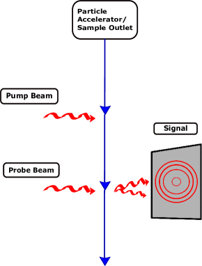
Figure 1: Schematic of the proposed experimental setup: Samples are accelerated to a fixed energy. A pump pulse and a probe pulse are directed parallel to each other and perpendicular to the sample direction of motion. The delay between the pump pulse and probe pulse can be controlled by changing the distance between the two beams.

III.1.2 Sample suitability

This novel method has its own set of unique challenges. To start with, it can only be applied to ions or molecules that are electrically charged so that they can be accelerated to relativistic speeds and are in the gas phase so they can reach the required energies. Moreover, the higher the mass of the sample the higher energy is required to run the experiment for a given time resolution. So, light, charged molecules and ions would be best suited for such studies.
The typical number density in gas phase UEDCenturion (2016); Yang and Centurion (2015); Shen et al. (2019) and spectroscopyBrünken et al. (2019) experiments is $\sim$ $10^{15}$ cm^-3. Proton bunches at the LHC contain $1.15$ $\times$ $10^{11}$ protons with a proton number density of $\sim$ $10^{16}$ cm^-3.Zimmermann et al. (2010); Steerenberg (2017) Many bunch length reduction schemes have been proposed and indeed an order of magnitude shorter bunch length has been produced for the purposes of accelerating electrons using plasma wakefields of proton bunches.Adli et al. (2018)
Another characteristic of a suitable sample is stability in the specific accelerator conditions. H- anions with a binding energy of $\sim$ 0.75 eV are accelerated regularly to 520 MeV at TRIUMF.TRIUMF Covalent bonds of molecules typically have binding energies on the order of 1 eV or higher.
Although originally designed to accelerate protons or positively charged ions only, the LHC ring has recently accelerated partially stripped Pb⁺⁸¹ ions with one electron to an energy of 6.5 Q TeV,Schaumann et al. (2019) where Q is the ion charge number as part of the gamma factory proposalWitold Krasny (2018) to create a new type of high intensity light source. Engineering challenges with respect to collimation are currently being addressed.Gorzawski et al. (2020)

III.2 Theoretical considerations

III.2.1 Energy considerations

Currently, the Large Hadron Collider at CERN can accelerate protons to energies on the order of 7 TeVFartoukh et al. (2020) and lead ions to a collision energy of 5 TeV,Foka and Janik (2016) which is enough to make remarkable gains in time resolution. As an example, a hydronium molecule ($H_{3}O^{+}$, rest mass: $3.16\times 10^{-26}$ kg) accelerated to an energy of $1.8$ TeV would experience a slowing down of time with a $\gamma$ factor of $100$. Since

$$E=\gamma mc^{2},$$ (3)

the time resolution scales proportionally to energy, so an energy of $18$ TeV would result in an astonishing $\gamma=1000$. Also, the time resolution is inversely proportional to mass so hydrogen ions, for example, would experience an order of magnitude higher gain in time resolution than hydronium molecules with the same energy.
Even if these particle accelerators cannot be commissioned to run this type of experiment in the near future it will still be extremely interesting to observe the effect of relativistic time dilation on dynamical processes. With current laser technology it is possible to observe changes in differential detection, with and without a perturbation, as small as $10^{-4}$ to $10^{-8}$Koke et al. (2010); Quinlan et al. (2013) using standard modulation techniques and photon detectors. There has also been major advances in laser based particle accelerators up to field gradients as high as $100$ GeV/mEsarey, Schroeder, and Leemans (2009); Leemans et al. (2014); Joshi, Corde, and Mori (2020); Blumenfeld et al. (2007) that will soon enable particle kinetic energies up to $10$ GeV range or higher. This degree of relativistic energy would lead to only modest time dilation compared to what can be achieved at particle accelerators. Nevertheless, this time retardation would be directly measurable and would provide an important test case for further advances in laser based particle acceleration with the goal of directly controlling the time variable, asymptotically approaching ’stopping’ time. This control of the time variable has the potential of opening new avenues beyond simple imaging to driving novel dynamics that would otherwise be too rapid to control.

III.2.2 Pump and probe beam dynamics

Pulsed pump and probe beams can be used as in standard ultrafast studies. The time resolution is mainly determined by the pulse duration of the pump and probe pulses. The pump pulse determines how fast a dynamic can be triggered and the probe pulse determines the imaging time resolution. The pulse duration conventionally refers to the time during which the full width at half max (FWHM) of the pulse crosses the sample. Other factors that affect time resolution are velocity mismatchCharles Williamson and Zewail (1993); Goodno, Astinov, and Miller (1999) that take place due to difference in velocity between the pump and probe pulses and due to their different incidence angles, and time of arrival jitterCenturion (2016) for RF accelerated electron pulses. However, due to the experimental geometry lower resolution due to velocity mismatch or time of arrival jitter is avoided as both pulses are parallel so the delay time from time zero is solely determined by the speed of the sample between the pump and probe pulses. In our proposed setup the pulse crosses the sample in two directions, and hence, we will consider the pulse duration, during which the pulse crosses the sample or vice versa, in both directions. To explain the physics we denote the direction, parallel to the direction of propagation of the sample beam, $y$ and denote the perpendicular direction $x$. We will treat the problem from the lab frame of reference as well as from the sample frame of reference for clarification.

Lab frame of reference

The pulse duration in the $x$-direction $\tau_{x}$ is given by

$$\tau_{x}=\frac{l_{x}}{v_{p}},$$ (4)

where $l_{x}$ indicates the pulse length in the $x$-direction and $v_{p}$ indicates the speed of the pump/probe pulse. The pulse duration in the $y$-direction $\tau_{y}$ is given by

$$\tau_{y}=\frac{l_{y}}{v_{s}},$$ (5)

where $l_{y}$ indicates the pulse length in the $y$-direction and $v_{s}$ indicates the speed of the sample. In the proposed experiment $v_{s}$ will always be close to the speed of light $c$.

Sample frame of reference

As samples reach relativistic speeds close to the speed of light the effect of length contraction along the direction of sample propagation $y$ becomes significant. Hence, the length of the pulse in the $y$-direction is contracted to

$$l^{{}^{\prime}}_{y}=\frac{l_{y}}{\gamma}.$$ (6)

The pulse duration in the $y$-direction $\tau^{{}^{\prime}}_{y}$ is then given by

$$\tau^{{}^{\prime}}_{y}=\frac{l_{y}}{\gamma v_{s}}.$$ (7)

The pulse duration in the $x$-direction $\tau^{{}^{\prime}}_{x}$ is given by

$$\tau^{{}^{\prime}}_{x}=\frac{\gamma l_{x}}{v_{p}}$$ (8)

as $v_{p}$ transforms to

$$v^{{}^{\prime}}_{p}=\frac{v_{p}}{\gamma}$$ (9)

in the sample frame of reference. This is due to relativistic angle aberration. A pulse that is emitted at $90^{\circ}$ in the lab frame of reference does not hit the sample perpendicularly in the sample frame of reference. The closer $v_{s}$ is to $c$ the smaller is the incidence angle between the beam and the sample’s line of motion in the sample frame of reference. Relativistic angular aberration will be discussed in more detail when discussing the observable signal. Typical pulses are Gaussian temporally and spatially ($\tau_{x}$ $\cong$ $\tau_{y}$) and so the time resolution $\tau_{res}$ would be determined by the relativistically shortened duration $\tau^{{}^{\prime}}_{y}$. It would thus be given by

$$\tau_{res}=\frac{1}{\gamma}\sqrt{\tau^{2}_{pump}+\tau^{2}_{probe}},$$ (10)

where $\tau_{pump}$ and $\tau_{probe}$ are the transit time durations of the sample beam through the pump and probe pulses in the lab frame, respectively. As an example for pump and probe beams with $l_{y}=10$ $\mu$m and $\gamma=100$, the time resolution would be roughly 470 as. Figure 2 shows a visual representation from both frames of reference along the relevant direction $y$.

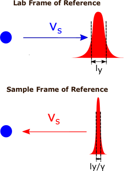
Figure 2: Lab and sample frames of reference: Along the $y$-direction the length of the pulse is contracted in the sample frame of reference relative to the lab frame of reference

In conventional pump-probe experiments the lab frame of reference is the same as the sample frame of reference. A signal (e.g. diffraction pattern) always reflects the interaction time according to the clock rate of the sample and hence, our proposed setup takes advantage of the involved relativistic effects that result from the differences between the two frames of reference.

III.2.3 Doppler effect and frequency shifts

It is of significant importance to understand how the frequency of a laser, x-ray or electron pulse, which is created in the lab frame, is ’seen’ by the sample in its own rest frame in order to properly carry out the experiment. For lasers, a significant shift in frequency may push it outside the absorption spectrum of the sample and hence, the intended interaction would not take place. For scattering x-rays and electrons, if they undergo significant redshift, for example, their spatial resolution would decrease. Relativistically, in addition to the classical Doppler effect, there is the added effect of time dilation. Even if the source and receiver are not crossing paths, relativity dictates a frequency shift known as transverse Doppler effect.Mandelberg and Witten (1962)
If we let $\theta$ be the angle between the sample wave vector and the wave vector of the pump/probe particles, as measured in the lab frame of reference, then the frequency that the sample ’sees’, $f_{s}$, is given in terms of the frequency in the lab frame of reference, $f_{l}$, by

$$f_{s}=f_{l}\gamma(1-\beta\cos{\theta})$$ (11)

for photons.Klein et al. (1992) For other particles, e.g. electrons, one needs to replace $\beta$ with

$$\beta_{e}=\frac{v_{s}}{v_{e}},$$ (12)

where $v_{e}$ is the speed of the particles but $\gamma=1/\sqrt{1-v_{s}^{2}/c^{2}}$ remains the same. In our proposed setup, where the pump and probe beams are perpendicular to the direction of motion of the samples, we have

$$f_{s}=f_{l}\gamma.$$ (13)

In fact, depending on the angle, there could either be a redshift or a blueshift. There is no frequency shift for one critical angle $\theta_{c}$. For $\beta$ ($\beta_{e}$) $\approx$ $1$, as $\gamma$ becomes larger, $\theta_{c}$ becomes smaller, meaning that the two wave vectors are more collinear. Although this would eliminate frequency shifts entirely, it would decrease the time resolution significantly.

III.2.4 The observable signal

Light can interact with matter in many different ways (e.g. absorption, scattering, etc.). In this section we present a general scheme for calculating the final observable signal in our proposed experiment.
The main steps are: (1) Transforming the incident field from the lab frame of reference to the sample frame of reference by applying the Lorentz transformations; (2) Calculating the resultant signal in the sample frame of reference; (3) Transforming the signal from the sample frame of reference to the lab frame of reference by applying the Lorentz transformations one more time.
Without loss of generality, for an incident electric field $E_{i}$ with angular frequency $\omega_{i}$ polarized in the z-direction and incident at angle $\theta_{i}$ (angle between photon wave vector $\vec{k_{i}}$ and sample velocity vector $\vec{v_{s}}$), the field would be Lorentz transformed to the sample frame of reference to $E^{{}^{\prime}}_{i}$ in the following way:Lee and Mittra (1967); Papas (1965)

$$\vec{E_{i}}=\hat{z}E_{i}\exp{[ik_{i}(\cos{\theta_{i}y}+sin{\theta_{i}x})]}\exp{(-i\omega_{i}t)},$$ (14)

$$\vec{E^{{}^{\prime}}_{i}}=\hat{z}^{{}^{\prime}}E^{{}^{\prime}}_{i}\exp{[ik_{i}^{{}^{\prime}}(\cos{\theta_{i}^{{}^{\prime}}y^{{}^{\prime}}}+sin{\theta_{i}^{{}^{\prime}}x^{{}^{\prime}}})]}\exp{(-i\omega^{{}^{\prime}}_{i}t^{{}^{\prime}})},$$ (15)

where

$$E^{{}^{\prime}}_{i}=\gamma(1-\beta\cos{\theta_{i}})E_{i},$$ (16)

$$k^{{}^{\prime}}_{i}=\frac{\omega^{{}^{\prime}}_{i}}{c},$$ (17)

$$\omega^{{}^{\prime}}_{i}=\gamma(1-\beta\cos{\theta_{i}})\omega_{i},$$ (18)

$$\theta^{{}^{\prime}}_{i}=\cos^{-1}{[\frac{\cos{\theta_{i}}-\beta}{1-\cos{\theta_{i}}(\beta)}]}.$$ (19)

For particles other than photons moving with speed $v_{e}$ the angular frequency and angle transform in the following way:

$$\omega^{{}^{\prime}}_{i}=\gamma(1-\beta_{e}\cos{\theta_{i}})\omega_{i},$$ (20)

$$\theta^{{}^{\prime}}_{i}=\tan^{-1}{[\frac{\sin{\theta_{i}}}{\gamma(\cos{\theta_{i}}-\beta_{e})}]}.$$ (21)

However, as before $\gamma=1/\sqrt{1-\beta^{2}}$ with $\beta=\frac{v_{s}}{c}$ remains the same.
Due to the nature of the angular transformations, we expect scattering and diffraction angles to be wider than for the static case, and hence, we recommend detectors that cover as much of the 4$\pi$ sr solid angle as possible.

IV Conclusion

We proposed a new method for time resolved studies that relies on taking advantage of relativistic effects rather than on advances in laser and electron beam compression technology. We have shown that our method has the potential of improving time resolutions by $2$ or $3$ orders of magnitude using currently available technology. This has the potential of unlocking a whole new domain of ultrafast dynamics that was previously unattainable. In a future that is pointing towards ever more powerful accelerators there will be a huge potential to achieve truly remarkable time resolutions that exceed the status quo by orders of magnitude. We hope this paper will open up new avenues of collaboration between the particle physics community and the ultrafast science community that would result in maximizing the research potential of particle accelerator facilities worldwide.

V Acknowledgments

H.D. would like to thank Prof. Pierre Savaria and Prof. David Bailey for fruitful discussions.

VI Data Availability

Data sharing is not applicable to this article as no new data were created or analyzed in this study.

References

- Miller (2014) R. J. D. Miller, Science 343, 1108 (2014).
- Miller (2016) R. J. D. Miller, in 13th International Conference on Fiber Optics and Photonics (Optical Society of America, 2016) p. P1A.25.
- Sciaini and Miller (2011) G. Sciaini and R. J. D. Miller, Rep. Prog. Phys. 74, 096101 (2011).
- Polanyi and Zewail (1995) J. C. Polanyi and A. H. Zewail, Accounts of Chemical Research 28, 119 (1995).
- Corkum and Krausz (2007) P. B. Corkum and F. Krausz, Nature Physics 3, 381–387 (2007).
- Barends et al. (2015) T. R. M. Barends, L. Foucar, A. Ardevol, K. Nass, A. Aquila, S. Botha, R. B. Doak, K. Falahati, E. Hartmann, M. Hilpert, and et al., Science 350, 445–450 (2015).
- Altarelli (2006) M. Altarelli, ed., XFEL, the European X-ray free-electron laser: technical design report (DESY XFEL Project Group, Hamburg, 2006) oCLC: 254657183.
- Siwick et al. (2002) B. J. Siwick, J. R. Dwyer, R. E. Jordan, and R. J. D. Miller, Journal of Applied Physics 92, 1643–1648 (2002).
- Ruan et al. (2004) C.-Y. Ruan, V. A. Lobastov, F. Vigliotti, S. Chen, and A. H. Zewail, Science 304, 80–84 (2004).
- Rosker, Dantus, and Zewail (1988) M. J. Rosker, M. Dantus, and A. H. Zewail, Science 241, 1200–1202 (1988).
- Mokhtari et al. (1990) A. Mokhtari, P. Cong, J. L. Herek, and A. H. Zewail, Nature 348, 225–227 (1990).
- Emma et al. (2010) P. Emma, R. Akre, J. Arthur, R. Bionta, C. Bostedt, J. Bozek, A. Brachmann, P. Bucksbaum, R. Coffee, F.-J. Decker, and et al., Nature Photonics 4, 641–647 (2010).
- Siwick et al. (2003) B. J. Siwick, J. R. Dwyer, R. E. Jordan, and R. J. D. Miller, Science 302, 1382–1385 (2003).
- Veisz et al. (2007) L. Veisz, G. Kurkin, K. Chernov, V. Tarnetsky, A. Apolonski, F. Krausz, and E. Fill, New Journal of Physics 9, 451–451 (2007).
- van Oudheusden et al. (2007) T. van Oudheusden, E. F. de Jong, S. B. van der Geer, W. P. E. M. O. t Root, O. J. Luiten, and B. J. Siwick, Journal of Applied Physics 102, 093501 (2007).
- Daoud, Floettmann, and Miller (2017) H. Daoud, K. Floettmann, and R. J. D. Miller, Struct. Dyn. 4, 044016 (2017).
- Hastings et al. (2006) J. B. Hastings, F. M. Rudakov, D. H. Dowell, J. F. Schmerge, J. D. Cardoza, J. M. Castro, S. M. Gierman, H. Loos, and P. M. Weber, Applied Physics Letters 89, 184109 (2006).
- Murooka et al. (2011) Y. Murooka, N. Naruse, S. Sakakihara, M. Ishimaru, J. Yang, and K. Tanimura, Applied Physics Letters 98, 251903 (2011).
- Musumeci et al. (2010) P. Musumeci, J. T. Moody, C. M. Scoby, M. S. Gutierrez, M. Westfall, and R. K. Li, Journal of Applied Physics 108, 114513 (2010).
- Baum and Zewail (2006) P. Baum and A. H. Zewail, Proceedings of the National Academy of Sciences 103, 16105–16110 (2006).
- Badali and Dwayne Miller (2017) D. S. Badali and R. J. Dwayne Miller, Structural dynamics (Melville, N.Y.) 4, 054302 (2017).
- Kassier et al. (2010) G. Kassier, K. Haupt, N. Erasmus, E. Rohwer, H. von Bergmann, H. Schwoerer, S. Coelho, and F. Auret, The Review of scientific instruments 81, 105103 (2010).
- Hassan et al. (2017) M. T. Hassan, J. S. Baskin, B. Liao, and A. H. Zewail, Nature Photonics 11, 425 (2017).
- Centurion (2016) M. Centurion, Journal of Physics B: Atomic, Molecular and Optical Physics 49, 062002 (2016).
- Yang and Centurion (2015) J. Yang and M. Centurion, Structural Chemistry 26, 1513–1520 (2015).
- Shen et al. (2019) X. Shen, J. P. F. Nunes, J. Yang, R. K. Jobe, R. K. Li, M.-F. Lin, B. Moore, M. Niebuhr, S. P. Weathersby, T. J. A. Wolf, and et al., Structural Dynamics 6, 054305 (2019).
- Brünken et al. (2019) S. Brünken, F. Lipparini, A. Stoffels, P. Jusko, B. Redlich, J. Gauss, and S. Schlemmer, The Journal of Physical Chemistry A 123, 8053–8062 (2019).
- Zimmermann et al. (2010) F. Zimmermann, R. Assmann, M. Giovannozzi, Y. Papaphilippou, A. Caldwell, and G. Xia, in Particle Accelerator Conference (PAC 09) (2010) p. FR5RFP004.
- Steerenberg (2017) R. Steerenberg, “LHC report: full house for the LHC,” (2017).
- Adli et al. (2018) E. Adli, A. Ahuja, O. Apsimon, R. Apsimon, A.-M. Bachmann, D. Barrientos, F. Batsch, J. Bauche, V. K. Berglyd Olsen, M. Bernardini, and et al., Nature 561, 363–367 (2018).
- (31) TRIUMF, “Main cyclotron and beam lines,” Accessed: 2021-01-27.
- Schaumann et al. (2019) M. Schaumann, R. Alemany-Fernandez, H. Bartosik, T. Bohl, R. Bruce, G. H. Hemelsoet, S. Hirlaender, J. M. Jowett, V. Kain, M. W. Krasny, and et al., Journal of Physics: Conference Series 1350, 012071 (2019).
- Witold Krasny (2018) M. Witold Krasny (Gamma Factory group), PoS EPS-HEP2017, 532 (2018).
- Gorzawski et al. (2020) A. Gorzawski, A. Abramov, R. Bruce, N. Fuster-Martinez, M. Krasny, J. Molson, S. Redaelli, and M. Schaumann, Physical Review Accelerators and Beams 23 (2020).
- Fartoukh et al. (2020) S. Fartoukh, N. Karastathis, L. Ponce, M. Solfaroli Camillocci, and R. Tomas Garcia, “About flat telescopic optics for the future operation of the lhc,” Tech. Rep. (CERN, 2020).
- Foka and Janik (2016) P. Foka and M. A. Janik, Reviews in Physics 1, 154–171 (2016).
- Koke et al. (2010) S. Koke, C. Grebing, H. Frei, A. Anderson, A. Assion, and G. Steinmeyer, Nature Photonics 4, 462–465 (2010).
- Quinlan et al. (2013) F. Quinlan, T. M. Fortier, H. Jiang, A. Hati, C. Nelson, Y. Fu, J. C. Campbell, and S. A. Diddams, Nature Photonics 7, 290–293 (2013).
- Esarey, Schroeder, and Leemans (2009) E. Esarey, C. B. Schroeder, and W. P. Leemans, Rev. Mod. Phys. 81, 1229 (2009).
- Leemans et al. (2014) W. P. Leemans, A. J. Gonsalves, H.-S. Mao, K. Nakamura, C. Benedetti, C. B. Schroeder, C. Tóth, J. Daniels, D. E. Mittelberger, S. S. Bulanov, J.-L. Vay, C. G. R. Geddes, and E. Esarey, Phys. Rev. Lett. 113, 245002 (2014).
- Joshi, Corde, and Mori (2020) C. Joshi, S. Corde, and W. B. Mori, Physics of Plasmas 27, 070602 (2020).
- Blumenfeld et al. (2007) I. Blumenfeld, C. E. Clayton, F.-J. Decker, M. J. Hogan, C. Huang, R. Ischebeck, R. Iverson, C. Joshi, T. Katsouleas, N. Kirby, and et al., Nature 445, 741–744 (2007).
- Charles Williamson and Zewail (1993) J. Charles Williamson and A. H. Zewail, Chemical Physics Letters 209, 10–16 (1993).
- Goodno, Astinov, and Miller (1999) G. D. Goodno, V. Astinov, and R. J. D. Miller, The Journal of Physical Chemistry B 103, 603–607 (1999).
- Mandelberg and Witten (1962) H. I. Mandelberg and L. Witten, Journal of the Optical Society of America 52, 529 (1962).
- Klein et al. (1992) R. Klein, R. Grieser, L. Hoog, G. Huber, I. Klaft, P. Merz, T. K Hl, S. Schr Der, M. Grieser, D. Habs, and et al., Zeitschrift f r Physik A Hadrons and Nuclei 342, 455–461 (1992).
- Lee and Mittra (1967) S. W. Lee and R. Mittra, Canadian Journal of Physics 45, 2999–3007 (1967).
- Papas (1965) C. H. Papas, Theory of electromagnetic wave propagation (McGraw-Hill Book Co., 1965).