EHT tests of the strong-field regime of General Relativity
Abstract
Following up on a recent analysis by Psaltis et al. [Phys. Rev. Lett. 125, 141104 (2020)], we show that the observed shadow size of M87∗ can be used to unambiguously and robustly constrain the black hole geometry in the vicinity of the circular photon orbit. Constraints on the post-Newtonian weak-field expansion of the black hole’s metric are instead more subtle to obtain and interpret, as they rely on combining the shadow-size measurement with suitable theoretical priors. We provide examples showing that post-Newtonian constraints resulting from shadow-size measurements should be handled with extreme care. We also discuss the similarities and complementarity between the EHT shadow measurements and black-hole gravitational quasi-normal modes.
Until the LIGO/Virgo detection of gravitational waves (GWs) Abbott and et al. (2016a, b, 2017a, 2017b, 2017c, 2020); Abbott et al. (2020a, b, c), General Relativity (GR) had only been tested in the solar system (characterized by weak gravitational fields and mildly relativistic velocities ) Will (2018) and in binary pulsars (which have strong gravitational fields inside/near the two stars, but again mildly relativistic orbital velocities ) Damour and Taylor (1992). Since in both cases , these tests are normally performed within the post-Newtonian formalism (i.e. an expansion in powers of ) Blanchet (2014). The advent of GW astronomy has pushed these tests to the strong-field and highly relativistic regime that characterizes merging BH binaries Abbott and et al. (2016c); Abbott et al. (2019, 2020d), where the PN formalism breaks down (except in the early-inspiral phase).
After coalescence, the BH merger remnant is expected to “ring down” by emitting quasi-normal modes (QNMs) Kokkotas and Schmidt (1999); Nollert (1999); Berti et al. (2009), i.e. damped oscillations with discrete frequencies and damping times, functions of the BH mass and spin only (because of the no-hair theorem Israel (1967); Hawking (1972); Carter (1971); Robinson (1975)). Therefore, by measuring two QNMs, one can in principle test the no-hair theorem and thus GR Dreyer et al. (2004); Berti et al. (2009). These tests are not yet possible with current detectors Berti et al. (2016) (even though there are clues of a second mode – and namely the first overtone of the dominant mode – besides the dominant QNM Giesler et al. (2019)). However, comparatively weaker inspiral-ringdown self-consistency tests, which compare the post-merger data to the signal predicted by GR by extrapolating the inspiral, show currently no hints of deviations from binary BHs in GR Abbott and et al. (2016c); Abbott et al. (2019, 2020d).
On larger scales, Psaltis et al. Psaltis et al. (2020) proposed using the shadow size of M to constrain deviations of the BH geometry from GR (i.e. to test the no-hair theorem). The EHT shadow-size measurement is consistent (to within 17% at 68-percentile confidence level) with the GR prediction111Like Psaltis et al. (2020), we assume that the shadow rim is associated with the photon sphere (i.e., for Schwarzschild BHs, the circular photon orbit). This is supported by simulations of the accretion flow onto M Akiyama et al. (2019a). If this identification is not exact (see §5.3, 7.3, and Appendix D of Akiyama et al. (2019a), cf. Gralla et al. (2019); Gralla (2020)), it will lead to larger errors in our analysis and in that of Psaltis et al. (2020). based on the object’s mass-to-distance ratio derived from stellar dynamics Akiyama et al. (2019b, c); Psaltis et al. (2020). Therefore, Psaltis et al. (2020) concludes that theories extending/modifying GR cannot yield shadow sizes differing by more than 17% (at 68% confidence) from the GR (i.e. Schwarzschild/Kerr) prediction Psaltis et al. (2020).222This optimistically neglects possible correlations of the parameters regulating deviations from GR with those of the BH (mass and spin) and accretion flow, which are fixed in Psaltis et al. (2020). These correlations may be important, as shown e.g. in Cardenas-Avendano et al. (2019) for tests of GR with X-ray observations.
While this idea is not new Takahashi (2005); Johannsen and Psaltis (2010); Psaltis and Johannsen (2011); Amarilla and Eiroa (2012); Broderick et al. (2014); Psaltis et al. (2015); Johannsen et al. (2016); Psaltis et al. (2016); Cunha et al. (2015, 2017); Psaltis (2019); Cunha et al. (2019); Medeiros et al. (2020), Psaltis et al. Psaltis et al. (2020) used it to constrain the BH geometry at 2PN order and beyond. To allow for deviations of the BH geometry from the Schwarzschild/Kerr solutions of GR, Psaltis et al. (2020) utilizes parametrized metrics Johannsen and Psaltis (2011); Johannsen (2013a); Vigeland et al. (2011); Johannsen (2013b); Rezzolla and Zhidenko (2014) that yield the usual PN expansion far from the BH, but which might be valid also in the strong-field region, where the PN expansion fails. Psaltis et al. (2020) also assumes that only one of the parameters that regulate deviations from GR in these metrics is non-zero and allowed to vary.
We will show that bounds on PN coefficients such as those obtained by Psaltis et al. (2020) depend sensitively on the assumed form of the parametrized BH metric. This is not surprising, as the results of Psaltis et al. (2020) rely on a single measurement (the shadow’s size). We will show instead that EHT shadow-size measurements can robustly constrain the BH geometry in the strong-field regime (near the circular photon orbit) and that these constraints are complementary to those from GW observations of QNMs.
Throughout this paper, we use units and metric signature .
EHT constraints on the PN expansion of BH geometries: As an example, we focus on the non-spinning parametrized geometry of Rezzolla and Zhidenko (RZ) Rezzolla and Zhidenko (2014) (see Konoplya et al. (2016); Younsi et al. (2016) for the axisymmetric generalization).333We neglect the spin as our goal is to discuss the robustness of the M87∗ shadow-size constraints with respect to the parametrization of the non-GR effects. The component is
| (1) |
with ( being the horizon’s radius), and
| (2) |
where is the mass and the dots represent a continued fraction structure. The Schwarzschild limit is recovered when (with ). When expanded in orders of , one recovers the usual PN structure
| (3) |
where the parameters depend on and vanish in the Schwarzschild limit. However, the continued-fraction structure of Eq. (2) is introduced to accelerate the convergence of the PN expansion (i.e. to “resum” it), so that the RZ metric aims to provide an accurate description even in the strong-field regime.
Null geodesics in a static, spherically symmetric geometry satisfy Bardeen (1973)
| (4) | ||||
| (5) |
where is the derivative (with respect to an affine parameter ) of the tortoise coordinate (defined by , with the areal radius), and (with and the photon’s conserved energy and angular momentum) is the impact parameter. The circular photon orbit’s radius, , and its impact parameter, , correspond to a minimum of the effective potential, i.e. they solve . These conditions can be reduced to Psaltis et al. (2020)
| (6) | ||||
| (7) |
which can be solved numerically for generic metrics; the Schwarzschild metric gives and . If is interpreted as the measured shadow size (like in Psaltis et al. (2020)), the EHT shadow-size measurement bounds at 68% confidence Psaltis et al. (2020).
The implications of this bound for the BH geometry depend on our prior knowledge of its functional form. For instance, if we assume Eq. (3) with all PN coefficients set to zero except for the 2PN term, i.e. for and flat priors for , one obtains the posterior distribution for shown in the first panel (left half) of Fig. 1. However, consider the RZ metric, imposing agreement with GR at 1PN order (; we will comment on this assumption below) and setting for for simplicity. With the four non-zero parameters , , and (for which we assume large flat priors of ), the posterior distribution for
| (8) |
is extremely broad (first panel of Fig. 1, right half). Similar conclusions hold for the higher PN terms whose expressions we do not show as lengthy and uninformative. In the second and third panels of Fig. 1, we show similar bounds for the 3PN and 4PN coefficients and , both when they are considered optimistically as the only free parameters [one at a time, via the metric (3)], and when their posteriors are instead obtained from those of the parameters , , and . All results of Fig. 1 were produced with the Metropolis-Hastings sampler of PyMC3 Salvatier et al. (2016), assuming Gaussian errors on the EHT shadow-size measurement. The bounds of Fig. 1 are reminiscent of those presented in Fig. 7 of Abbott and et al. (2016c) by the LIGO/Virgo collaboration for the PN coefficients of the BH-binary inspiral GW signal.444See also Cardenas-Avendano et al. (2020) for GW bounds on the PN coefficients of the conservative dynamics, which are stronger than those claimed by Psaltis et al. (2020) although comparable directly to them (because like Psaltis et al. (2020), Cardenas-Avendano et al. (2020) assumes only one free non-GR parameter). Indeed, our approach resembles closely that of Abbott and et al. (2016c), i.e. “optimistic” bounds are obtained by letting those PN coefficients free one by one, while “pessimistic” bounds assume that they are all allowed to vary simultaneously. We stress that correlations between the PN coefficients, when several of them are allowed to vary simultaneously, also appear in the case of GW measurements. However, unlike our case, the LIGO/Virgo “pessimistic” posteriors are smaller than the priors, at least for the leading-order (0PN) term in the GW phase, cf. Table I of Abbott and et al. (2016c) (see also Sampson et al. (2013); Yunes et al. (2016); Psaltis et al. (2021)). This will be even more true for the -1PN term Barausse et al. (2016); Abbott et al. (2019). Note also that the conclusions of our Fig. 1 (and namely that the “pessimistic” bounds on the single PN parameters—while marginalizing on all others—coincide with the priors) are robust against inclusion of lower-PN orders (e.g. ).
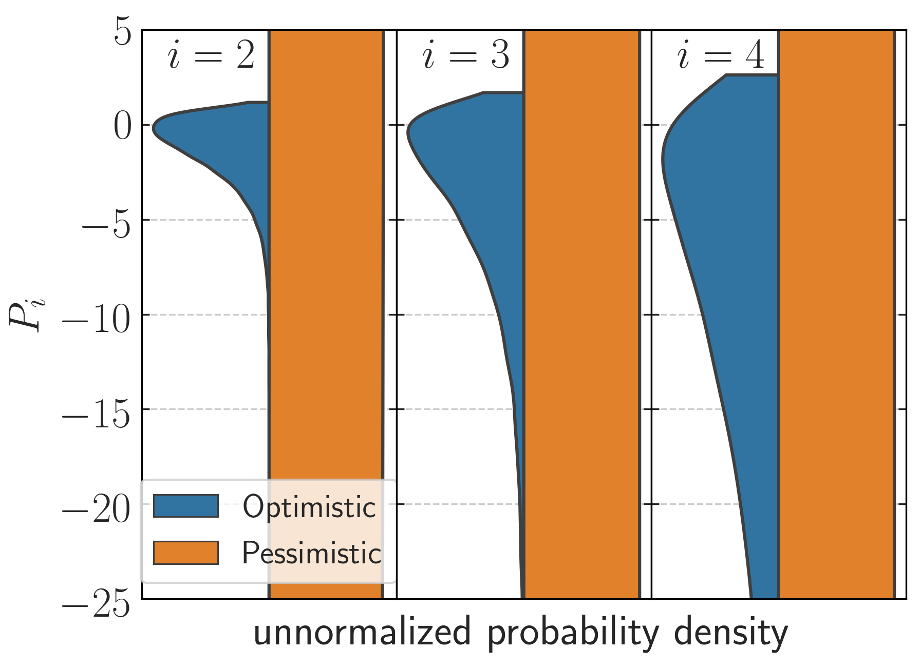
Fig. 1 shows that the bounds of Psaltis et al. (2020) are not robust, but depend on the form of the parametrized metric and on the priors on its parameters. To illustrate how subtle it is to put priors on the shape and PN coefficients of parametrized metrics, let us stress that even though we have followed above Psaltis et al. (2020) and required to match the Schwarzschild solution at 1PN order (i.e. ), there is in principle no reason to do so. While Psaltis et al. (2020) sets 1PN deviations from GR to zero, theories different from GR do not necessarily satisfy Birkhoff’s theorem Berti et al. (2015) and may not obey the strong-equivalence principle Barausse et al. (2016). Therefore, the metric around BHs need not be the same as around a star, and one cannot invoke solar-system tests to set the 1PN deviations from GR to zero. While this was mentioned in Psaltis et al. (2020), the implications of the assumption of vanishing 1PN deviations from GR was not explored (Psaltis et al. (2020) simply mentions that as a “very conservative” assumption). We will now explore cases where that assumption is not verified and affects the bounds that one obtains.
An example is given by a theory with a “dark photon” [i.e. a U(1) gauge field], possibly coupled with a scalar Garfinkle et al. (1991); Hirschmann et al. (2018):
| (9) |
This is known as Einstein-Maxwell-dilaton theory [if the U(1) symmetry is broken, e.g. by a light mass, the dark photon may even be the dark matter; cf. McDermott and Witte (2020) and references therein]. Spherical BHs in this theory are described by a generalized Reissner-Nordström metric. The component reads Gibbons and Maeda (1988); Garfinkle et al. (1991)
| (10) |
where the areal radius is , and the constants are related to the mass and the dark charge of the BH through and . Unlike an electric charge, which is neutralized by the plasma near the horizon Barausse et al. (2014), may be non-zero and different for a BH (where it is a free parameter) and a star (where it vanishes unless the dark photon and/or the scalar are coupled to the Standard Model). Obviously, for and the metric (10) deviates from Schwarzschild at 1PN order.
EHT strong-field tests of gravity: We stress that the behavior of Fig. 1 – and namely the fact that the (marginalized) pessimistic bounds on the PN coefficients coincide with the priors – is not only due to the larger number of parameters being varied. In fact, irrespective of how many parameters the model (i.e. the parametrized metric) has, the shadow size does constrain a particular combination of the parameters. We show this explicitly in Fig. 2, where we plot the posteriors for and (evaluated at ) in the “pessimistic” scenario of Fig. 1.555We assume here a 5% precision for the shadow-size measurement, which may be achievable with next-generation EHT-like experiments Raymond et al. (2021), to show that these conclusions will not change with better future data. This shows that the data is informative and that the inference can be robust against the number of parameters involved, as long as one asks the right question (i.e. as long as one does not attempt to estimate the PN coefficients, but focuses instead on the geometry near the circular photon orbit). Conversely, the geometry away from the circular photon orbit (even in its immediate vicinity) is less constrained, as shown by the posteriors at and plotted in Fig. 2. This plot therefore highlights that the behavior of the PN constraints of Fig. 1 is due to the slow convergence (if any) of PN expansion near the circular photon orbit.
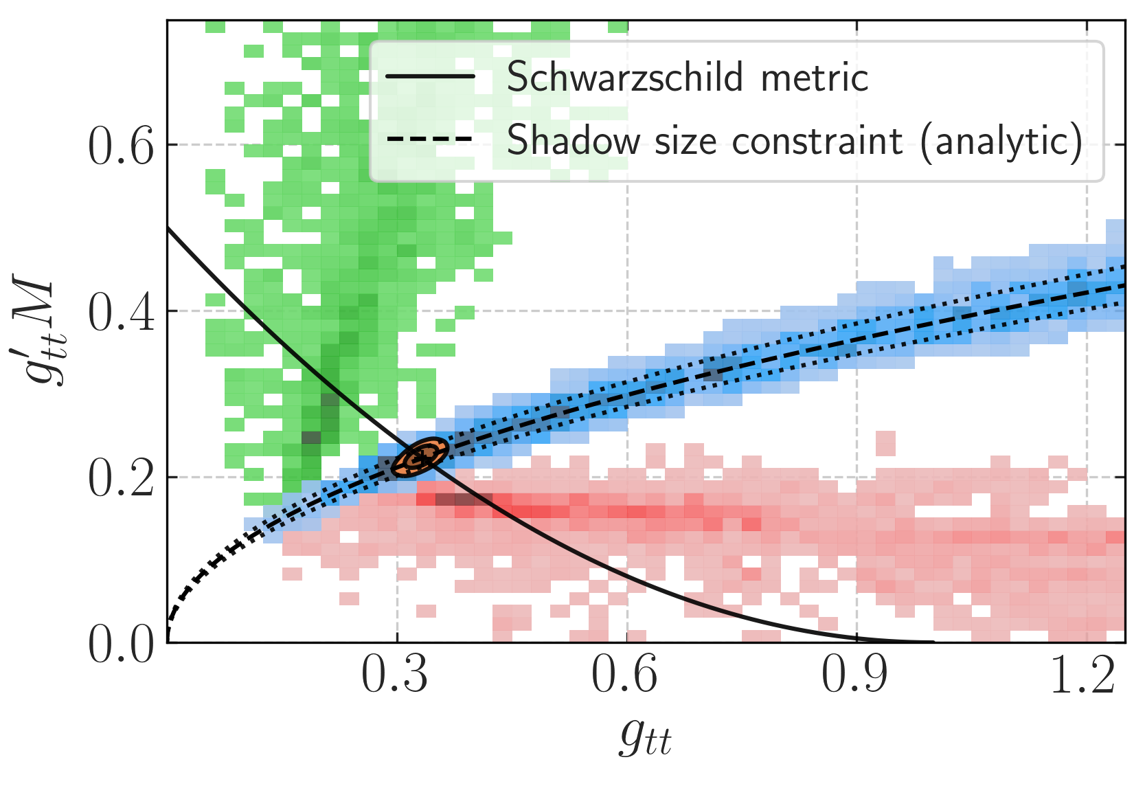
As correctly stated in Psaltis et al. (2020), “if more than one PN parameter […] is included, then the size measurement of the BH shadow will […] lead to a constraint on a linear combination of these parameters.” However, the combination in question is nothing but itself (as shown by the solid and dashed lines in Fig. 2), and becomes linear only if deviations of the PN coefficients from their GR values are small (which is not obvious). Under this assumption, however, one can solve Eqs. (6)–(7) by inserting the PN metric (3) and linearizing in the . One then obtains that the EHT bound is approximately (at 68% confidence and assuming vanishing BH spin)
| (11) |
We stress that the coefficients of this combination will be different for non-vanishing spin. In fact, since for high spins the circular photon orbit approaches (in Boyer-Lindquist coordinates) the horizon Bardeen (1973), we expect those coefficients to all be comparable.
This approximate constraint explains the growing width of the “optimistic” bounds of Fig. 1 as the PN order increases. It also suggests that bounds on the lowest-order PN parameters (0PN Abbott and et al. (2016c) and -1PN Barausse et al. (2016); Abbott et al. (2019)) from GW observations of the early inspiral of BH binaries are potentially stronger than than those from shadow-size measurements, even though posterior correlations may still appear at higher-PN orders, when several parameters are varied at the same time Abbott and et al. (2016c); Shoom et al. (2021). In more detail, GW detectors are sensitive to a whole time (or frequency) series, unlike the EHT shadow-size observation (which amounts to a single data point). They measure, in particular, the GW phase , where is the GR-predicted phase, the GW frequency, the binary total mass, and the are parameters accounting for deviations from GR at (integer) PN orders Yunes and Pretorius (2009); Cornish et al. (2011); Chatziioannou et al. (2012); Yunes et al. (2016); Abbott and et al. (2016c); Abbott et al. (2019); Cardenas-Avendano et al. (2020) (in the GR limit, and for ). Since (with the orbital separation), the phase is a series in , just like Eq. (11). The difference with Eq. (11) is that BH-binary inspiral observations are sensitive to separations from tens of down to , which accelerates convergence. Similarly, X-ray observations of accretion disks around BHs Bambi and Barausse (2011); Bambi (2017); Tripathi et al. (2019); Nampalliwar et al. (2019); Cardenas-Avendano et al. (2020) are sensitive to radii larger than the innermost stable circular orbit, thus being in a regime where the PN expansion is applicable (although bounds derived from these observations may depend on the accretion-disk model Riaz et al. (2020); Abdikamalov et al. (2020); Cardenas-Avendano et al. (2019)).
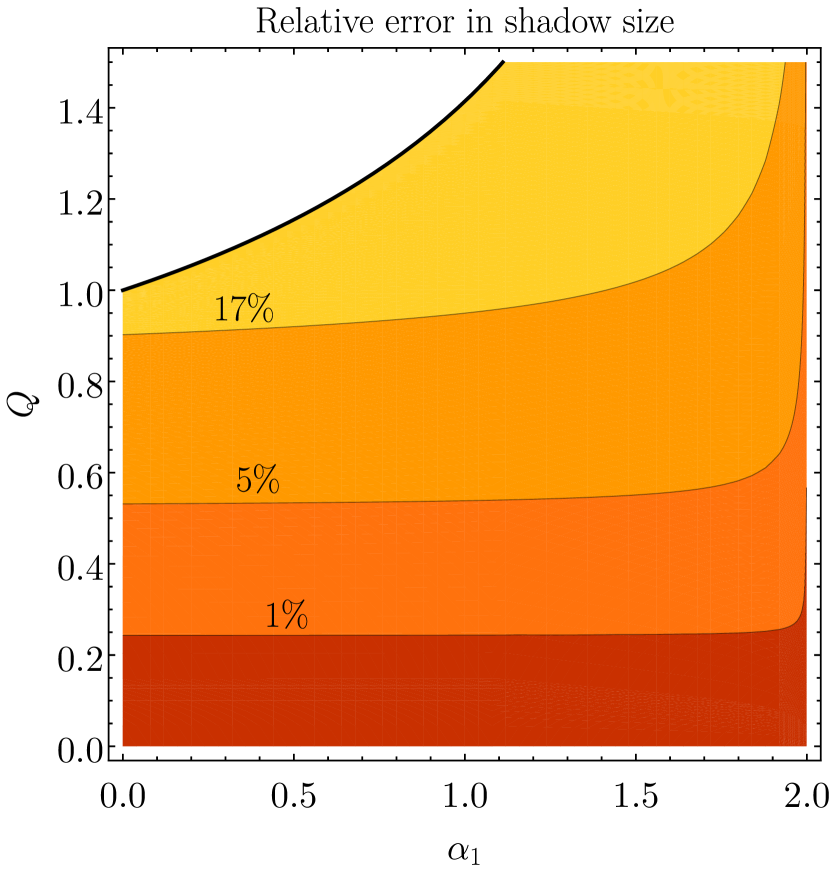
An alternative way to exploit EHT observations is to consider BH solutions in gravitational theories different from GR, which are often known exactly and/or numerically and which will in general show deviations from the Schwarzschild/Kerr metric at all PN orders. To show this explicitly, we will present a few examples, making (like above) the simplifying assumption of spherical symmetry.666Such a theory-by-theory approach is not needed in situations where the PN expansion is well suited for the system at hand and yields robust bounds. This is the case e.g. for solar-system tests, for which parametric bounds on the 1PN coefficients are robust and can be readily converted into constraints on specific theories. Consider first the Reissner-Nordström-like BH of Eq. (10). If , that reduces exactly to the Reissner-Nordström spacetime, which features for . The EHT shadow-size measurement then bounds in the 68% confidence interval . In the general case, the solution is governed by two independent parameters: the coupling and the BH charge . The fractional difference between and the Schwarzschild value is shown in Fig. 3, with the region within the 17% contour being in agreement with the EHT shadow-size measurement. From these bounds, one may then obtain posteriors for the PN coefficients, whose confidence intervals are , , , .
Hairy BHs differing from the Schwarzschild one can also be obtained in scalar-tensor theories, provided that a coupling between the scalar and the Gauss-Bonnet invariant is introduced, giving rise theories known as Einstein-scalar-Gauss-Bonnet gravity. Their action is Julié and Berti (2019)
| (12) |
with a coupling constant (with dimensions of a length) and a dimensionless coupling function. Provided that is monotonic, one can find BH solutions characterized by a dimensionless scalar charge, defined from the decay of the scalar near spatial infinity, being the BH mass and the asymptotic value of the scalar field. For these theories , where a prime denotes the derivative with respect to . Numerical solutions can be found for specific coupling functions, e.g. Kanti et al. (1996); Pani and Cardoso (2009), or Sotiriou and Zhou (2014a, b). Alternatively, one can find solutions perturbatively in the charge for various monotonic coupling functions Mignemi and Stewart (1993); Yunes and Stein (2011); Maselli et al. (2015); Julié and Berti (2019). Using the fits of Kokkotas et al. (2017) to the numerical solutions of Kanti et al. (1996) [for ], we find that these BHs always agree with the EHT shadow-size measurement if the precision of the measurement is worse than . This confirms the findings of Cunha et al. (2017).
Interesting solutions can also be found for non-monotonic coupling functions. If has a minimum, BHs can scalarize spontaneously in Einstein-scalar-Gauss-Bonnet gravity Silva et al. (2018); Doneva and Yazadjiev (2018); Antoniou et al. (2018); Cunha et al. (2019); Collodel et al. (2020); Herdeiro et al. (2020); Berti et al. (2020). These scalarized BHs form because the Schwarzschild and/or Kerr solutions of GR become tachyonically unstable in these theories Silva et al. (2018); Doneva and Yazadjiev (2018); Andreou et al. (2019); Minamitsuji and Ikeda (2019); Dima et al. (2020); Doneva et al. (2020a, b).
Consider the case , studied in Cunha et al. (2019); Doneva and Yazadjiev (2018). This theory provides a continuum set of scalarized BHs with mass . The EHT shadow-size measurement then constrains (see also Cunha et al. (2019))777We expect to agree with early-inspiral GW observations (because as : cf. Doneva and Yazadjiev (2018), Fig. 4), although merger/ringdown bounds have not been derived yet.. While this bound is not new (having been derived in Cunha et al. (2019), cf. their Fig. 5), one can compare it with the results of our Fig. 1 for the RZ parametrized metric. The PN expansion of scalarized BHs (obtained by solving the field equations perturbatively near spatial infinity) yields PN parameters , , , . Moreover, an additional coupling of the scalar to the Ricci curvature can even give rise to Antoniou et al. (2021). The charge is a function of , and can be extracted from the numerical solutions to the full field equations. The EHT bound then translates into the constraint and thus , , . As can be seen, in this specific case the bounds on the PN parameters are comparable to (or even better than) the “optimistic” bounds of Fig. 1.
Discussion: We stress that the dependence of the shadow-size bounds on the PN coefficients on how many of them are allowed to vary, as well as the robustness of the constraints on the geometry near the circular photon orbit are reminiscent of what happens with GW observations of QNMs in the ringdown phase of binary BHs. Indeed, shadow-size measurements are to the EHT what QNMs are to GW detectors. Both shadows and QNMs are sensitive to the BH geometry near the circular photon orbit, and their physics cannot be described within the PN approximation. Note that Völkel and Barausse (2020) attempted to constrain parametrized metrics (e.g. the RZ metric) with QNM observations. In agreement with this letter, Völkel and Barausse (2020) found that constraints on the reconstructed geometry are robust near the peak of the effective potential. We show this explictly in Fig. 2, where we present projected QNM constraints on and , alongside those from the shadow size mentioned earlier, in the “pessimistic” case where the four non-zero parameters , , and are allowed to vary simultaneously.
In more detail, the geometric-optics limit of the GW propagation equation reduces, in GR, to the null-geodesics one (see e.g., Völkel and Barausse (2020)), i.e., high-frequency gravitational wavefronts follow null geodesics. Therefore, the effective potential for QNMs in the geometric-optics limit (i.e., the limit of large angular eigen-numbers ) coincides with that of null geodesics [Eq. (4)]. Since QNMs are generated at the peak of the effective potential, which is close to the circular photon orbit (and coincides with it for ), it is not surprising that the QNM frequencies of the Kerr spacetime are given (in the geometric-optics limit) by linear combinations of the orbital and frame-dragging precession frequencies of the circular null orbit (or simply by multiples of the orbital frequency in Schwarzschild, where the two frequencies coincide) Goebel (1972); Ferrari and Mashhoon (1984); Schutz and Will (1985); Yang et al. (2012). Similarly, one can relate QNM decay times to the Lyapunov exponents of null geodesics near the circular photon orbit Cardoso et al. (2009); Ferrari and Mashhoon (1984); Schutz and Will (1985); Yang et al. (2012). These exponents depend in turn on the curvature of the effective potential for photon orbits near its peak.
This null geodesics/QNMs correspondence can be generalized to BH spacetimes different from Kerr/Schwarzschild, at least in a wide class of gravitational theories Glampedakis et al. (2017); Glampedakis and Silva (2019); Silva and Glampedakis (2020); Völkel and Barausse (2020). This correspondence motivates combining EHT shadow-size tests of the no-hair theorem with the QNM null tests of the same theorem that will become possible with third-generation GW interferometers or spaced-based detectors such as e.g., LISA Berti et al. (2016) or TianQin Shi et al. (2019).
Acknowledgements.
Acknowledgments: S.V., E.B. and N.F. acknowledge financial support provided under the European Union’s H2020 ERC Consolidator Grant “GRavity from Astrophysical to Microscopic Scales” grant agreement no. GRAMS-815673. This work was supported in part by Perimeter Institute for Theoretical Physics. Research at Perimeter Institute is supported by the Government of Canada through the Department of Innovation, Science and Economic Development Canada and by the Province of Ontario through the Ministry of Economic Development, Job Creation and Trade. A.E.B. thanks the Delaney Family for their generous financial support via the Delaney Family John A. Wheeler Chair at Perimeter Institute. A.E.B. and receives additional financial support from the Natural Sciences and Engineering Research Council of Canada through a Discovery Grant. We thank A. Cardenas Avendano, E. Berti, K. Glampedakis, R. Gold, P. Kocherlakota, K. D. Kokkotas, L. Rezzolla, N. Wex and N. Yunes for insightful conversations and for reviewing a draft of this manuscript. During the completion of this work we have become aware of a related work by P. Kocherlakota, L. Rezzolla, et al., which deals with topics that partly overlap with those of this manuscript (i.e. EHT bounds on exact non-GR BH solutions).References
- Abbott and et al. (2016a) B. P. Abbott and et al. (LIGO Scientific Collaboration and Virgo Collaboration), Phys. Rev. Lett. 116, 061102 (2016a).
- Abbott and et al. (2016b) B. P. Abbott and et al. (LIGO Scientific Collaboration and Virgo Collaboration), Phys. Rev. Lett. 116, 241103 (2016b).
- Abbott and et al. (2017a) B. P. Abbott and et al. (LIGO Scientific and Virgo Collaboration), Phys. Rev. Lett. 118, 221101 (2017a).
- Abbott and et al. (2017b) B. P. Abbott and et al., The Astrophysical Journal 851, L35 (2017b).
- Abbott and et al. (2017c) B. P. Abbott and et al. (LIGO Scientific Collaboration and Virgo Collaboration), Phys. Rev. Lett. 119, 141101 (2017c).
- Abbott and et al. (2020) B. P. Abbott and et al., The Astrophysical Journal 892, L3 (2020).
- Abbott et al. (2020a) R. Abbott et al. (LIGO Scientific, Virgo), (2020a), arXiv:2004.08342 [astro-ph.HE] .
- Abbott et al. (2020b) R. Abbott et al. (LIGO Scientific, Virgo), Astrophys. J. Lett. 896, L44 (2020b), arXiv:2006.12611 [astro-ph.HE] .
- Abbott et al. (2020c) R. Abbott et al. (LIGO Scientific, Virgo), Phys. Rev. Lett. 125, 101102 (2020c), arXiv:2009.01075 [gr-qc] .
- Will (2018) C. M. Will, Theory and Experiment in Gravitational Physics (Cambridge University Press, 2018).
- Damour and Taylor (1992) T. Damour and J. H. Taylor, Phys. Rev. D 45, 1840 (1992).
- Blanchet (2014) L. Blanchet, Living Rev. Rel. 17, 2 (2014), arXiv:1310.1528 [gr-qc] .
- Abbott and et al. (2016c) B. P. Abbott and et al. (LIGO Scientific and Virgo Collaborations), Phys. Rev. Lett. 116, 221101 (2016c).
- Abbott et al. (2019) B. Abbott et al. (LIGO Scientific, Virgo), Phys. Rev. D 100, 104036 (2019), arXiv:1903.04467 [gr-qc] .
- Abbott et al. (2020d) R. Abbott et al. (LIGO Scientific, Virgo), (2020d), arXiv:2010.14529 [gr-qc] .
- Kokkotas and Schmidt (1999) K. D. Kokkotas and B. G. Schmidt, Living Rev. Rel. 2, 2 (1999), arXiv:gr-qc/9909058 .
- Nollert (1999) H.-P. Nollert, Classical and Quantum Gravity 16, R159 (1999).
- Berti et al. (2009) E. Berti, V. Cardoso, and A. O. Starinets, Classical and Quantum Gravity 26, 163001 (2009).
- Israel (1967) W. Israel, Phys. Rev. 164, 1776 (1967).
- Hawking (1972) S. Hawking, Commun. Math. Phys. 25, 152 (1972).
- Carter (1971) B. Carter, Phys. Rev. Lett. 26, 331 (1971).
- Robinson (1975) D. Robinson, Phys. Rev. Lett. 34, 905 (1975).
- Dreyer et al. (2004) O. Dreyer, B. J. Kelly, B. Krishnan, L. S. Finn, D. Garrison, and R. Lopez-Aleman, Class. Quant. Grav. 21, 787 (2004), arXiv:gr-qc/0309007 .
- Berti et al. (2016) E. Berti, A. Sesana, E. Barausse, V. Cardoso, and K. Belczynski, Phys. Rev. Lett. 117, 101102 (2016), arXiv:1605.09286 [gr-qc] .
- Giesler et al. (2019) M. Giesler, M. Isi, M. A. Scheel, and S. Teukolsky, Phys. Rev. X 9, 041060 (2019), arXiv:1903.08284 [gr-qc] .
- Psaltis et al. (2020) D. Psaltis et al. (EHT Collaboration), Phys. Rev. Lett. 125, 141104 (2020).
- Akiyama et al. (2019a) K. Akiyama et al. (Event Horizon Telescope), Astrophys. J. Lett. 875, L5 (2019a), arXiv:1906.11242 [astro-ph.GA] .
- Gralla et al. (2019) S. E. Gralla, D. E. Holz, and R. M. Wald, Phys. Rev. D 100, 024018 (2019), arXiv:1906.00873 [astro-ph.HE] .
- Gralla (2020) S. E. Gralla, (2020), arXiv:2010.08557 [astro-ph.HE] .
- Akiyama et al. (2019b) K. Akiyama et al. (Event Horizon Telescope), Astrophys. J. 875, L1 (2019b), arXiv:1906.11238 [astro-ph.GA] .
- Akiyama et al. (2019c) K. Akiyama et al. (Event Horizon Telescope), Astrophys. J. Lett. 875, L6 (2019c), arXiv:1906.11243 [astro-ph.GA] .
- Cardenas-Avendano et al. (2019) A. Cardenas-Avendano, J. Godfrey, N. Yunes, and A. Lohfink, Phys. Rev. D 100, 024039 (2019), arXiv:1903.04356 [gr-qc] .
- Takahashi (2005) R. Takahashi, Publ. Astron. Soc. Jap. 57, 273 (2005), arXiv:astro-ph/0505316 .
- Johannsen and Psaltis (2010) T. Johannsen and D. Psaltis, Astrophys. J. 718, 446 (2010), arXiv:1005.1931 [astro-ph.HE] .
- Psaltis and Johannsen (2011) D. Psaltis and T. Johannsen, J. Phys. Conf. Ser. 283, 012030 (2011), arXiv:1012.1602 [astro-ph.HE] .
- Amarilla and Eiroa (2012) L. Amarilla and E. F. Eiroa, Phys. Rev. D 85, 064019 (2012), arXiv:1112.6349 [gr-qc] .
- Broderick et al. (2014) A. E. Broderick, T. Johannsen, A. Loeb, and D. Psaltis, Astrophys. J. 784, 7 (2014), arXiv:1311.5564 [astro-ph.HE] .
- Psaltis et al. (2015) D. Psaltis, F. Ozel, C.-K. Chan, and D. P. Marrone, Astrophys. J. 814, 115 (2015), arXiv:1411.1454 [astro-ph.HE] .
- Johannsen et al. (2016) T. Johannsen, A. E. Broderick, P. M. Plewa, S. Chatzopoulos, S. S. Doeleman, F. Eisenhauer, V. L. Fish, R. Genzel, O. Gerhard, and M. D. Johnson, Phys. Rev. Lett. 116, 031101 (2016), arXiv:1512.02640 [astro-ph.GA] .
- Psaltis et al. (2016) D. Psaltis, N. Wex, and M. Kramer, Astrophys. J. 818, 121 (2016), arXiv:1510.00394 [astro-ph.HE] .
- Cunha et al. (2015) P. V. P. Cunha, C. A. R. Herdeiro, E. Radu, and H. F. Runarsson, Phys. Rev. Lett. 115, 211102 (2015), arXiv:1509.00021 [gr-qc] .
- Cunha et al. (2017) P. V. Cunha, C. A. R. Herdeiro, B. Kleihaus, J. Kunz, and E. Radu, Phys. Lett. B 768, 373 (2017), arXiv:1701.00079 [gr-qc] .
- Psaltis (2019) D. Psaltis, Gen. Rel. Grav. 51, 137 (2019), arXiv:1806.09740 [astro-ph.HE] .
- Cunha et al. (2019) P. V. Cunha, C. A. Herdeiro, and E. Radu, Phys. Rev. Lett. 123, 011101 (2019), arXiv:1904.09997 [gr-qc] .
- Medeiros et al. (2020) L. Medeiros, D. Psaltis, and F. Özel, Astrophys. J. 896, 7 (2020), arXiv:1907.12575 [astro-ph.HE] .
- Johannsen and Psaltis (2011) T. Johannsen and D. Psaltis, Phys. Rev. D 83, 124015 (2011), arXiv:1105.3191 [gr-qc] .
- Johannsen (2013a) T. Johannsen, Phys. Rev. D 87, 124017 (2013a).
- Vigeland et al. (2011) S. Vigeland, N. Yunes, and L. C. Stein, Phys. Rev. D 83, 104027 (2011).
- Johannsen (2013b) T. Johannsen, Phys. Rev. D 88, 044002 (2013b).
- Rezzolla and Zhidenko (2014) L. Rezzolla and A. Zhidenko, Phys. Rev. D 90, 084009 (2014).
- Konoplya et al. (2016) R. Konoplya, L. Rezzolla, and A. Zhidenko, Phys. Rev. D 93, 064015 (2016), arXiv:1602.02378 [gr-qc] .
- Younsi et al. (2016) Z. Younsi, A. Zhidenko, L. Rezzolla, R. Konoplya, and Y. Mizuno, Phys. Rev. D 94, 084025 (2016), arXiv:1607.05767 [gr-qc] .
- Bardeen (1973) J. Bardeen, in Les Houches Summer School of Theoretical Physics: Black Holes (1973) pp. 215–240.
- Salvatier et al. (2016) J. Salvatier, T. V. Wiecki, and C. Fonnesbeck, PeerJ Computer Science 2, e55 (2016).
- Cardenas-Avendano et al. (2020) A. Cardenas-Avendano, S. Nampalliwar, and N. Yunes, Class. Quant. Grav. 37, 135008 (2020), arXiv:1912.08062 [gr-qc] .
- Sampson et al. (2013) L. Sampson, N. Cornish, and N. Yunes, Phys. Rev. D 87, 102001 (2013), arXiv:1303.1185 [gr-qc] .
- Yunes et al. (2016) N. Yunes, K. Yagi, and F. Pretorius, Phys. Rev. D 94, 084002 (2016), arXiv:1603.08955 [gr-qc] .
- Psaltis et al. (2021) D. Psaltis, C. Talbot, E. Payne, and I. Mandel, Phys. Rev. D 103, 104036 (2021), arXiv:2012.02117 [gr-qc] .
- Barausse et al. (2016) E. Barausse, N. Yunes, and K. Chamberlain, Phys. Rev. Lett. 116, 241104 (2016), arXiv:1603.04075 [gr-qc] .
- Berti et al. (2015) E. Berti et al., Class. Quant. Grav. 32, 243001 (2015), arXiv:1501.07274 [gr-qc] .
- Garfinkle et al. (1991) D. Garfinkle, G. T. Horowitz, and A. Strominger, Phys. Rev. D 43, 3140 (1991), [Erratum: Phys.Rev.D 45, 3888 (1992)].
- Hirschmann et al. (2018) E. W. Hirschmann, L. Lehner, S. L. Liebling, and C. Palenzuela, Phys. Rev. D 97, 064032 (2018), arXiv:1706.09875 [gr-qc] .
- McDermott and Witte (2020) S. D. McDermott and S. J. Witte, Phys. Rev. D 101, 063030 (2020), arXiv:1911.05086 [hep-ph] .
- Gibbons and Maeda (1988) G. Gibbons and K.-i. Maeda, Nucl. Phys. B 298, 741 (1988).
- Barausse et al. (2014) E. Barausse, V. Cardoso, and P. Pani, Phys. Rev. D 89, 104059 (2014), arXiv:1404.7149 [gr-qc] .
- Raymond et al. (2021) A. W. Raymond, D. Palumbo, S. N. Paine, L. Blackburn, R. Córdova Rosado, S. S. Doeleman, J. R. Farah, M. D. Johnson, F. Roelofs, R. P. J. Tilanus, and J. Weintroub, Astrophys. J. Suppl. 253, 5 (2021), arXiv:2102.05482 [astro-ph.IM] .
- Völkel and Barausse (2020) S. H. Völkel and E. Barausse, Phys. Rev. D 102, 084025 (2020), arXiv:2007.02986 [gr-qc] .
- Shoom et al. (2021) A. A. Shoom, P. K. Gupta, B. Krishnan, A. B. Nielsen, and C. D. Capano, (2021), arXiv:2105.02191 [gr-qc] .
- Yunes and Pretorius (2009) N. Yunes and F. Pretorius, Phys. Rev. D 80, 122003 (2009), arXiv:0909.3328 [gr-qc] .
- Cornish et al. (2011) N. Cornish, L. Sampson, N. Yunes, and F. Pretorius, Phys. Rev. D 84, 062003 (2011), arXiv:1105.2088 [gr-qc] .
- Chatziioannou et al. (2012) K. Chatziioannou, N. Yunes, and N. Cornish, Phys. Rev. D 86, 022004 (2012), [Erratum: Phys.Rev.D 95, 129901 (2017)], arXiv:1204.2585 [gr-qc] .
- Bambi and Barausse (2011) C. Bambi and E. Barausse, Astrophys. J. 731, 121 (2011), arXiv:1012.2007 [gr-qc] .
- Bambi (2017) C. Bambi, Rev. Mod. Phys. 89, 025001 (2017), arXiv:1509.03884 [gr-qc] .
- Tripathi et al. (2019) A. Tripathi, A. B. Abdikamalov, D. Ayzenberg, C. Bambi, and S. Nampalliwar, Phys. Rev. D 99, 083001 (2019), arXiv:1903.04071 [gr-qc] .
- Nampalliwar et al. (2019) S. Nampalliwar, S. Xin, S. Srivastava, A. B. Abdikamalov, D. Ayzenberg, C. Bambi, T. Dauser, J. A. Garcia, and A. Tripathi, (2019), arXiv:1903.12119 [gr-qc] .
- Riaz et al. (2020) S. Riaz, D. Ayzenberg, C. Bambi, and S. Nampalliwar, Mon. Not. Roy. Astron. Soc. 491, 417 (2020), arXiv:1908.04969 [astro-ph.HE] .
- Abdikamalov et al. (2020) A. B. Abdikamalov, D. Ayzenberg, C. Bambi, T. Dauser, J. A. Garcia, S. Nampalliwar, A. Tripathi, and M. Zhou, Astrophys. J. 899, 80 (2020), arXiv:2003.09663 [astro-ph.HE] .
- Julié and Berti (2019) F.-L. Julié and E. Berti, Phys. Rev. D 100, 104061 (2019), arXiv:1909.05258 [gr-qc] .
- Kanti et al. (1996) P. Kanti, N. Mavromatos, J. Rizos, K. Tamvakis, and E. Winstanley, Phys. Rev. D 54, 5049 (1996), arXiv:hep-th/9511071 .
- Pani and Cardoso (2009) P. Pani and V. Cardoso, Phys. Rev. D 79, 084031 (2009), arXiv:0902.1569 [gr-qc] .
- Sotiriou and Zhou (2014a) T. P. Sotiriou and S.-Y. Zhou, Phys. Rev. Lett. 112, 251102 (2014a), arXiv:1312.3622 [gr-qc] .
- Sotiriou and Zhou (2014b) T. P. Sotiriou and S.-Y. Zhou, Phys. Rev. D 90, 124063 (2014b), arXiv:1408.1698 [gr-qc] .
- Mignemi and Stewart (1993) S. Mignemi and N. Stewart, Phys. Rev. D 47, 5259 (1993), arXiv:hep-th/9212146 .
- Yunes and Stein (2011) N. Yunes and L. C. Stein, Phys. Rev. D 83, 104002 (2011), arXiv:1101.2921 [gr-qc] .
- Maselli et al. (2015) A. Maselli, P. Pani, L. Gualtieri, and V. Ferrari, Phys. Rev. D 92, 083014 (2015), arXiv:1507.00680 [gr-qc] .
- Kokkotas et al. (2017) K. Kokkotas, R. Konoplya, and A. Zhidenko, Phys. Rev. D 96, 064004 (2017), arXiv:1706.07460 [gr-qc] .
- Silva et al. (2018) H. O. Silva, J. Sakstein, L. Gualtieri, T. P. Sotiriou, and E. Berti, Phys. Rev. Lett. 120, 131104 (2018), arXiv:1711.02080 [gr-qc] .
- Doneva and Yazadjiev (2018) D. D. Doneva and S. S. Yazadjiev, Phys. Rev. Lett. 120, 131103 (2018), arXiv:1711.01187 [gr-qc] .
- Antoniou et al. (2018) G. Antoniou, A. Bakopoulos, and P. Kanti, Phys. Rev. Lett. 120, 131102 (2018), arXiv:1711.03390 [hep-th] .
- Collodel et al. (2020) L. G. Collodel, B. Kleihaus, J. Kunz, and E. Berti, Class. Quant. Grav. 37, 075018 (2020), arXiv:1912.05382 [gr-qc] .
- Herdeiro et al. (2020) C. A. Herdeiro, E. Radu, H. O. Silva, T. P. Sotiriou, and N. Yunes, (2020), arXiv:2009.03904 [gr-qc] .
- Berti et al. (2020) E. Berti, L. G. Collodel, B. Kleihaus, and J. Kunz, (2020), arXiv:2009.03905 [gr-qc] .
- Andreou et al. (2019) N. Andreou, N. Franchini, G. Ventagli, and T. P. Sotiriou, Phys. Rev. D 99, 124022 (2019), [Erratum: Phys.Rev.D 101, 109903 (2020)], arXiv:1904.06365 [gr-qc] .
- Minamitsuji and Ikeda (2019) M. Minamitsuji and T. Ikeda, Phys. Rev. D 99, 104069 (2019), arXiv:1904.06572 [gr-qc] .
- Dima et al. (2020) A. Dima, E. Barausse, N. Franchini, and T. P. Sotiriou, (2020), arXiv:2006.03095 [gr-qc] .
- Doneva et al. (2020a) D. D. Doneva, L. G. Collodel, C. J. Krüger, and S. S. Yazadjiev, (2020a), arXiv:2008.07391 [gr-qc] .
- Doneva et al. (2020b) D. D. Doneva, L. G. Collodel, C. J. Krüger, and S. S. Yazadjiev, (2020b), arXiv:2009.03774 [gr-qc] .
- Antoniou et al. (2021) G. Antoniou, A. Lehébel, G. Ventagli, and T. P. Sotiriou, (2021), arXiv:2105.04479 [gr-qc] .
- Goebel (1972) C. J. Goebel, Astrophys. J. Lett. 172, L95 (1972).
- Ferrari and Mashhoon (1984) V. Ferrari and B. Mashhoon, Phys. Rev. D 30, 295 (1984).
- Schutz and Will (1985) B. F. Schutz and C. M. Will, Astrophys. J. Lett. 291, L33 (1985).
- Yang et al. (2012) H. Yang, D. A. Nichols, F. Zhang, A. Zimmerman, Z. Zhang, and Y. Chen, Physical Review D 86 (2012), 10.1103/physrevd.86.104006.
- Cardoso et al. (2009) V. Cardoso, A. S. Miranda, E. Berti, H. Witek, and V. T. Zanchin, Phys. Rev. D 79, 064016 (2009), arXiv:0812.1806 [hep-th] .
- Glampedakis et al. (2017) K. Glampedakis, G. Pappas, H. O. Silva, and E. Berti, Physical Review D 96 (2017), 10.1103/physrevd.96.064054.
- Glampedakis and Silva (2019) K. Glampedakis and H. O. Silva, Phys. Rev. D 100, 044040 (2019), arXiv:1906.05455 [gr-qc] .
- Silva and Glampedakis (2020) H. O. Silva and K. Glampedakis, Phys. Rev. D 101, 044051 (2020), arXiv:1912.09286 [gr-qc] .
- Shi et al. (2019) C. Shi, J. Bao, H. Wang, J.-d. Zhang, Y. Hu, A. Sesana, E. Barausse, J. Mei, and J. Luo, Phys. Rev. D 100, 044036 (2019), arXiv:1902.08922 [gr-qc] .