Lightweight Single-Image Super-Resolution Network with Attentive Auxiliary Feature Learning

Abstract

Despite convolutional network-based methods have boosted the performance of single image super-resolution (SISR), the huge computation costs restrict their practical applicability. In this paper, we develop a computation efficient yet accurate network based on the proposed attentive auxiliary features (A²F) for SISR. Firstly, to explore the features from the bottom layers, the auxiliary feature from all the previous layers are projected into a common space. Then, to better utilize these projected auxiliary features and filter the redundant information, the channel attention is employed to select the most important common feature based on current layer feature. We incorporate these two modules into a block and implement it with a lightweight network. Experimental results on large-scale dataset demonstrate the effectiveness of the proposed model against the state-of-the-art (SOTA) SR methods. Notably, when parameters are less than 320k, A²F outperforms SOTA methods for all scales, which proves its ability to better utilize the auxiliary features. Codes are available at https://github.com/wxxxxxxh/A2F-SR.

1 Introduction

Convolutional neural network (CNN) has been widely used for single image super-resolution (SISR) since the debut of SRCNN [1]. Most of the CNN-based SISR models [2, 3, 4, 5, 6, 7] are deep and large. However, in the real world, the models often need to be run efficiently in embedded system like mobile phone with limited computational resources [8, 9, 10, 11, 12, 13]. Thus, those methods are not proper for many practical SISR applications, and lightweight networks have been becoming an important way for practical SISR. Also, the model compression techniques can be used in lightweight architecture to further reduce the parameters and computation. However, before using model compression techniques (e.g. model pruning), it is time-consuming to train a large model and it also occupies more memory. This is unrealistic for some low budget devices, so CNN-based lightweight SISR methods become increasingly popular because it can be regarded as an image preprocessing or postprocessing instrument for other tasks [14, 15, 16, 17, 18].

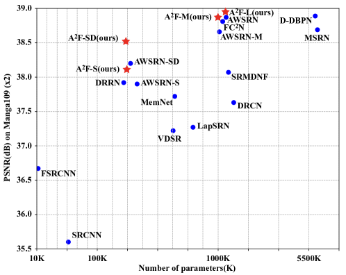
Figure 1: Cost-effectiveness comparison between the proposed A²F model variants (A²F-S, A²F-SD, A²F-M, A²F-L) with other methods on the Manga109 [19] on $\times$2 scale. The proposed models can achieve high PSNR with fewer parameters. Note that MSRN [20] and D-DBPN [21] are large models.

One typical strategy is to reduce the parameters [22, 23, 24, 25]. Moreover, the network architecture is essential for lightweight SISR models. Generally, methods of designing architectures can be categorized into two groups. One is based on neural architecture search. MoreMNA-S and FALSR [26, 27] adopt the evolutionary algorithm to search efficient model architectures for lightweight SISR. The other is to design the models manually [28, 29]. These methods all utilize features of previous layers to better learn the features of the current layer, which reflect that auxiliary features can boost the performance of lightweight models. However, these methods do not fully use all the features of previous layers, which possibly limits the performance.

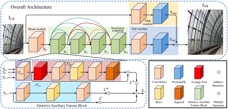
Figure 2: The architecture of A²F with 4 attentive auxiliary feature blocks. The architecture of A²F with more attentive auxiliary feature blocks is similar. Note that 1$\times$1 convolution kernel is used to project the auxiliary features and learn the importance of different channels of projected features. The convolution kernels elsewhere are all $3\times 3$. The input is the LR image and the output is the predicted HR image. Pixelshuffle [30] is used to upsample the features to the high-resolution image with target size.

Directly combining the auxiliary features with current features is conceptually problematic as features of different layers are often embedded in different space. Thus, we use the projection unit to project the auxiliary features to a common space that is suitable for fusing features. After projected to a common space, these projected features may not be all useful for learning features of the current layer. So we adopt the channel attention to make the model automatically assign the importance to different channels. The projection unit and channel attention constitute the proposed attentive auxiliary feature block. We term our model that consists of Attentive Auxiliary Feature blocks as A²F since it utilizes the auxilary features and the attention mechanism. Figure 1 gives the comparison between different models on Manga109 [19] dataset with a upscale factor of 2. As shown in Figure 1, models of our A²F family can achieve better efficiency than current SOTA methods [28, 29]. Figure 2 describes the architecture of A²F with four attentive auxiliary feature blocks. Our main contributions are given below:

• We handle the super resolution task from a new direction, which means we discuss the benefit brought by auxiliary features in the view of how to recover multi-frequency through different layers. Thus, we propose the attentive auxiliary feature block to utilize auxiliary features of previous layers for facilitating features learning of the current layer. The mainstay we use the channel attention is the dense auxiliary features rather than the backbone features or the sparse skip connections, which is different from other works.

• Compared with other lightweight methods especially when the parameters are less than 1000K, we outperform all of them both in PSNR and SSIM but have fewer parameters, which is an enormous trade-off between performance and parameters. In general, A²F is able to achieve better efficiency than current state-of-the-art methods [29, 28, 31].

• Finally, we conduct a thorough ablation study to show the effectiveness of each component in the proposed attentive auxiliary feature block. We release our PyTorch implementation of the proposed method and its pretrained models together with the publication of the paper.

2 Related Work

Instead of powerful computers with GPU, embedded devices usually need to run a super resolution model. As a result, lightweight SR architectures are needed and have been recently proposed.

One pioneering work is SRCNN [1] which contains three convolution layers to directly map the low-resolution (LR) images to high-resolution (HR) images. Subsequently, a high-efficiency SR model named ESPCNN [24] was introduced, which extracts feature maps in LR space and contains a sub-pixel convolution layer that replaces the handcrafted bicubic filter to upscale the final LR map into the HR images. DRRN [25] also had been proposed to alleviate parameters by adopting recursive learning while increasing the depth. Then CARN [32] was proposed to obtain an accurate but lightweight result. It addresses the issue about heavy computation by utilizing the cascading mechanism for residual networks. More recently, AWSRN [28] was designed to decrease the heavy computation. It applies the local fusion block for residual learning. For lightweight network, it can remove redundancy scale branches according to the adaptive weights.

Feature fusion has undergone its tremendous progress since the ResNet [33] was proposed, which implies the auxiliary feature is becoming the crucial aspect for learning. The full utilization of the auxiliary feature was adopted in DenseNet [34]. The authors take the feature map of each former layer into a layer, and this alleviates the vanishing gradient problem. SR methods also make use of auxiliary features to improve performance, such as [2, 25, 35, 7, 36]. The local fusion block of AWSRN [28] consists of concatenated AWRUs and a LRFU. Each output of AWRUs is combined one by one, which means a dense connection for a block. A novel SR method called FC²N was presented in [29]. A module named GFF was devised through implementing all skip connections by weighted channel concatenation, and it also can be considered as the auxiliary feature.

As an important technique for vision tasks, attention mechanism [37] can automatically determine which component is important for learning. Channel attention is a type of attention mechanism, which concentrates on the impact of each feature channel. SENet [38] is a channel attention based model in the image classification task. In the domain of SR, RCAN [7] had been introduced to elevate SR results by taking advantage of interdependencies among channels. It can adaptively rescale features according to the training target.

In our paper, auxiliaty features are not fully-dense connections, which indicates it is not dense in one block. We expect that each block can only learn to recover specific frequency information and provide auxiliary information to the next block. There are two main differences compred with FC²N and AWSRN. One is that for a block of A²F, we use the features of ALL previous blocks as auxiliary features of the current block, while FC²N and AWSRN use the features of a FIXED number of previous blocks. The second is that we adopt channel attention to decide how to transmit different informations to the next block, but the other two works do not adopt this mechanism.

3 Proposed Model

3.1 Motivation and Overview

Our method is motivated by an interesting fact that many CNN based methods [32, 3, 29] can reconstruct the high frequency details from the low resolution images hierachically, which indicates that different layers learn the capacity of recovering multi-frequency information. However, stacking more layers increases the computation burden and higher frequency information is difficult to regain. So we aim to provide a fast, low-parameters and accurate method that can restore more high frequency details on the basis of ensuring the accuracy of low frequency information reconstruction. According to this goal, we have the following observations:

• To build a lightweight network, how to diminish parameters and the multiply operation is essential. Generally, we consider reducing the depth or the width of the network, performing upsampling operation at the end of the network and adopting small kernel to reach this target. It also brings a new issue that a shallow network (i.e. fewer layers and fewer channels in each layer) can not have an excellent training result due to the lower complexity of the model, which also can be considered as an under-fitting problem.

• For the limited depth and width of the network, feature reusing is the best way to solve the issue. By this way, the low-frequency information can be transmitted to the next layer easily and it is more useful to combine multi-level low-frequency features to obtain accurate high-frequency features. Thus, more features benefitting to recover high-frequency signal will circulate across the entire network. It will promote the capacity of learning the mapping function if the network is shallow.

• We also consider another problem that the impact of multi-frequency information should be different when used for the learning of high frequency features. As the depth of the layer becomes deeper, effective information of the last layer provided for current layer is becoming rarer, because the learning of high frequency features is more and more difficult. So how to combine the information of all the previous layers to bring an efficient result is important and it should be dicided by the network.

Based on these observations, we design the model by reusing all features of the preceding layers and then concating them directly along channels like [34] in a block. Meanwhile, to reduce the disturbance brought by the redundant information when concating all of channels and adaptively obtain the multi-frequency reconstruction capability of different layers, we adopt the same-space attention mechanism in our model, which can avoid the situation that features from different space would cause extraodinary imbalance when computing the attention weight.

Table 1: Configurations of the proposed method. We set $stride=1$ for every convolutional operation to keep the same size in each layer. $i$ indicates the $i$-th A²F module and $p$ means the scale factor. For the A²F-SD model, we change the channels that are 32 in other models to 16 for each $\mathcal{F}$.

Function	Details	Kernel	Channels (Input, Output)
$\mathcal{F}_{head}$	Convolution	$3\times 3$	(3, 32)
$\mathcal{F}_{skip}$	Convolution	$3\times 3$	(3, $p*p*3$)
	PixelShuffle	-	-
$\mathcal{F}^{i}_{proj}$	Convolution	$1\times 1$	($i*32$, 32)
$\mathcal{F}^{i}_{att}$	Adaptive AvgPool	-	-
	Convolution	$1\times 1$	(32, 32)
	ReLU	-	-
	Convolution	$1\times 1$	(32, 32)
	Sigmoid	-	-
$\mathcal{F}^{i}_{res}$	Convolution	$3\times 3$	(32, 128)
	ReLU	-	-
	Convolution	$3\times 3$	(128, 32)
$\mathcal{F}_{tail}$	Convolution	$3\times 3$	(32, $p*p*3$)
	PixelShuffle	-	-

3.2 Overall Architecture

As shown in Figure 2, the whole model architecture is divided into four components: head module, nonlinear mapping, skip module and tail module. Detailed configuration of each component can be seen in Table 1. We denote the low resolution and the predicted image as $I_{LR}$ and $I_{SR}$, respectively. The input is first processed by the head module $\mathcal{F}_{head}$ to get the features $x_{0}$:

$$x_{0}=\mathcal{F}_{head}(I_{LR}),$$ (1)

and $\mathcal{F}_{head}$ is just one 3$\times$3 convolutional layer (Conv). We do not use $1\times 1$ Conv in the first layer for it can not capture the spatial correlation and cause a information loss of the basic low frequency. The reason why we use a $3\times 3$ Conv rather than a $5\times 5$ Conv is twofold: a) $3\times 3$ Conv can use fewer parameters to contribute to the lightweight of the network. b) It is not suitable to employ kernels with large receptive field in the task of super-resolution, especially for the first layer. Recall that each pixel in downsampled image corresponds to a mini-region in the original image. So during the training, large receptive field may introduce irrelevant information.

Then the nonlinear mapping which consists of $L$ stacked attentive auxiliary feature blocks is used to further extract information from $x_{0}$. In the $i_{th}$ attentive auxiliary feature block, the features $x_{i}$ is extracted from all the features of the previous blocks $x_{0},x_{1},x_{2},...,x_{i-1}$:

$$x_{i}=g^{i}_{AAF}(x_{0},x_{1},...,x_{i-1}),$$ (2)

where $g^{i}_{AAF}$ denotes attentive auxiliary feature block $i$.

After getting the features $x_{L}$ from the last attentive auxiliary feature block, $\mathcal{F}_{tail}$, which is a 3$\times$3 convolution layer followed by a pixelshuffle layer [24], is used to upsample $x_{L}$ to the features $x_{tail}$ with targe size:

$$x_{tail}=\mathcal{F}_{tail}(x_{L}).$$ (3)

We design this module to integrate the multi-frequency information produced by different blocks. It also correlates channels and spatial correlation, which is useful for pixelshuffle layer to rescale the image.

To make the mapping learning easier and introduce the original low frequency information to keep the accuracy of low frequency, the skip module $\mathcal{F}_{skip}$, which has the same component with $\mathcal{F}_{tail}$, is adopted to get the global residual information $x_{skip}$:

$$x_{skip}=\mathcal{F}_{skip}(I_{LR}).$$ (4)

Finally, the target $I_{SR}$ is obtained by adding $x_{skip}$ and $x_{tail}$:

$$I_{SR}=x_{tail}\oplus x_{skip}.$$ (5)

where $\oplus$ denotes the element-wise add operation.

3.3 Attentive Auxiliary Feature Block

The keypoint of the A²F is that it adopts attentive auxiliary feature blocks to utilize all the usable features. Given features $x_{0},x_{1},...,x_{i-1}$ from all previous blocks, it is improper to directly fuse with features of the current block because features of different blocks are in different feature spaces. Thus we need to project auxiliary features to a common-space that is suitable to be fused, which prevent features of different space from causing extraodinary imbalance for attention weights. In A²F, 1$\times$1 convolution layer $\mathcal{F}^{i}_{proj}$ is served as such a projection unit. The projected features of the $i_{th}$ auxiliary block $x^{proj}_{i}$ are obtained by

$$x^{proj}_{i}=\mathcal{F}^{i}_{proj}([x_{0},x_{1},...,x_{i-1}]),$$ (6)

where $[x_{0},x_{1},...,x_{i-1}]$ concatenates $x_{0},x_{1},...,x_{i-1}$ along the channel. However, different channels of $x^{proj}_{i}$ have different importance when being fused with features of current layer. Therefore, channel attention $\mathcal{F}^{i}_{att}$ is used to learn the importance factor of different channel of $x^{proj}_{i}$. In this way, we get the new features $x^{att}_{i}$ by

$$x^{att}_{i}=\mathcal{F}^{i}_{att}(x^{proj}_{i})\otimes x^{proj}_{i},$$ (7)

where $\mathcal{F}^{i}_{att}$ consists of one average pooling layer, one 1$\times$1 convolution layer, one ReLU layer, another 1$\times$1 convolution layer and one sigmoid layer. The symbol $\otimes$ means channel-wise multiplication. The block of WDSR_A [5] is adopted to get the features of current layer $x^{res}_{i}$:

$$x^{res}_{i}=\mathcal{F}^{i}_{res}(x_{i-1}),$$ (8)

where $\mathcal{F}^{i}_{res}$ consists of one 3$\times$3 convolution layer, one ReLU layer and another 3$\times$3 convolution layer. The output of $i_{th}$ attentive auxiliary feature block $x_{i}$ is given by:

$$x_{i}=\lambda^{res}_{i}\times x^{res}_{i}+\lambda^{att}_{i}\times x^{att}_{i}+\lambda^{x}_{i}\times x_{i-1},$$ (9)

where $\lambda^{res}_{i}$, $\lambda^{att}_{i}$ and $\lambda^{x}_{i}$ are feature factors for different features like [28]. These feature factors will be learned automatically when training the model. Here we choose additive operation for it can better handle the situation that the $\lambda^{att}_{i}$ of some auxiliary features is 0. If we concat channels directly, there will be some invalid channels which may increase the redundancy of the network. We can also reduce parameters by additive operation sin it does not expand channels.

4 Experiments

In this section, we first introduce some common datasets and metrics for evaluation. Then, we describe details of our experiment and analyze the effectiveness of our framework. Finally, we compare our model with state-of-the-art methods both in qualitation and quantitation to demonstrate the superiority of A²F. For more experiments please refer to the supplementary materials.

4.1 Dataset and Evaluation Metric

DIV2K dataset [39] with 800 training images is used in previous methods [28, 29] for model training. When testing the performance of the models, Peak Signal to Noise Ratio (PSNR) and the Structural SIMilarity index (SSIM) [40] on the Y channel after converting to YCbCr channels are calculated on five benchmark datasets including Set5 [41], Set14 [42], B100 [43], Urban100 [44] and Manga109 [19]. We also adopt the LPIPS [45] as a perceptual metric to do comparison, which can avoid the situation that over-smoothed images may present a higher PSNR/SSIM when the performances of two methods are similar.

4.2 Implementation Details

Similar to AWSRN [28], we design four variants of A²F, denoted as A²F-S, A²F-SD, A²F-M and A²F-L. The channels of $\mathcal{F}^{i}_{res}$ in the attentive auxiliary feature block of A²F-S, A²F-M and A²F-L are set to {32,128,32} channels, which means the input, internal and output channel number of $\mathcal{F}^{i}_{res}$ is 32, 128, 32, respectively. The channels of $\mathcal{F}^{i}_{res}$ in the attentive auxiliary feature block of A²F-SD is set to {16,128,16}. For the A²F-SD model, we change all of the channels that are setted as 32 in A²F-S, A²F-M, A²F-L to 16. The number of the attentive auxiliary feature blocks of A²F-S, A²F-SD, A²F-M and A²F-L is 4, 8, 12, and 16, respectively. During the training process, typical data augmentation including horizontal flip, rotation and random rotations of $90^{o}$, $180^{o}$, $270^{o}$ are used. The model is trained using Adam algorithm [46] with L1 loss. The initial value of $\lambda^{res}_{i}$, $\lambda^{att}_{i}$ and $\lambda^{x}_{i}$ are set to 1. All the code are developed using PyTorch on a machine with an NVIDIA 1080 Ti GPU.

4.3 Ablation Study

In this section, we first demonstrate the effectiveness of the proposed auxiliary features. Then, we conduct an ablation experiments to study the effect of essential components of our model and the selection of the kernel for the head component.

4.3.1 Effect of auxiliary features

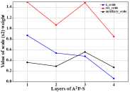
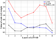
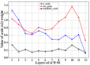
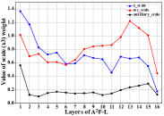
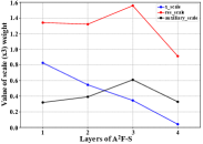
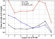
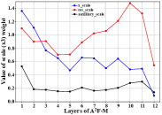
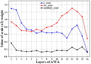
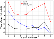
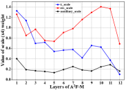
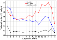
Figure 3: The weight of $\lambda^{res}_{i}$ (res_scale), $\lambda^{att}_{i}$ (auxiliary_scale) and $\lambda^{x}_{i-1}$ (x_scale) in different layers. From top to bottom are the results on the $\times 2$, $\times 3$, $\times 4$ tasks. From left to right are the results of models A²F-S, A²F-SD, A²F-M and A²F-L.

To show the effect of auxiliary features, we plot the $\lambda^{res}_{i}$, $\lambda^{att}_{i}$ and $\lambda^{x}_{i-1}$ of each layer of each model in Figure 3. As shown in Figure 3, the value of $\lambda^{att}_{i}$ are always bigger than 0.2, which reflects that the auxiliary features always play a certain role in generating the output features of the auxiliary features block. It can also be observed that in all the models of A²F, the weight of $x^{res}_{i}$ (i.e. $\lambda^{res}_{i}$) plays the most important role. The weight of $x_{i-1}$ (i.e. $\lambda^{x}_{i-1}$) is usually larger than $\lambda^{att}_{i}$. However, for the more lightweight SISR models (i.e. A²F-S and A²F-SD), $x^{att}_{i}$ becomes more and more important than $x_{i-1}$ (i.e. $\lambda^{att}_{i}$ becomes more and more larger than $\lambda^{x}_{i-1}$) as the number of layers increases. This reflects that auxiliary features may have great effects on the lightweight SISR models.

4.3.2 Effect of projection unit and channel attention

Table 2: Results of ablation study on the projection unit and the channel attention. PSNR is calculated on the super-resolution task with a scale factor of 2. PU means projection unit and CA means channel attention. “MP” in the model means more parameters.

Model	PU	CA	Param	MutiAdds	Set5	Set14	B100	Urban100	Manga109
BASELINE			1190K	273.9G	38.04	33.69	32.20	32.20	38.66
BASELINE-MP			1338K	308.0G	38.09	33.70	32.21	32.25	38.69
A2F-L-NOCA	$\surd$		1329K	306.0G	38.08	33.75	32.23	32.39	38.79
A2F-L-NOCA-MP	$\surd$		1368K	315.1G	38.09	33.77	32.23	32.35	38.79
A2F-L	$\surd$	$\surd$	1363K	306.1G	38.09	33.78	32.23	32.46	38.95

To evaluate the performance of the projection unit and channel attention in the attentive auxiliary feature block, WDSR_A [5] with 16 layers is used as the BASELINE model. Then we drop the channel attention in the attentive auxiliary feature block and such model is denoted as A²F-L-NOCA. To further prove the performance gain comes from the proposed attention module, we perform an experiment as follows: we increase the number of parameters of BASELINE and A²F-L-NOCA, and we denote these models as BASELINE-MP and A²F-L-NOCA-MP, where MP means more parameters. Table 2 shows that comparing the results of BASELINE, BASELINE-MP and A²F-L-NOCA, we can find that projection unit with auxiliary features can boost the performance on all the datasets. Comparing the results of A²F-L-NOCA, A²F-L-NOCA-MP, A²F-L, it can be found that channel attention in the attentive auxiliary feature block further improves the performance. Thus, we draw the conclusion that the projection unit and channel attention in the auxiliary can both better explore the auxiliary features. In our supplementary materials, we also do this ablation study on a challengeable case (i.e. A²F-S for x4) to show that the good using of auxiliary features is especially important for shallow networks.

Table 3: Results of ablation study on different kernel size which is only used for head component. Note that other convolutional kernels are same.

Convolutional Kernel Selection
Kernel	Parameters	Set5	Set14	B100	Urban100	Manga109
$1\times 1$	319.2K	32.00	28.46	27.46	25.78	30.13
$\bm{3\times 3}$	319.6K	32.06	28.47	27.48	25.80	30.16
$5\times 5$	320.4K	32.00	28.45	27.48	25.80	38.13
$7\times 7$	321.6K	31.99	28.44	27.48	25.78	30.10

4.3.3 Kernel selection for $\mathcal{F}_{head}$

We select different size of kernels in $\mathcal{F}_{head}$ to verify that $1\times 1$ conv and large receptive field are not suitable for the head component. From Table 3, we can observe both of them have whittled the performance of the network. This result verifies the reasonability of our head component which has been introduced in section 3.2

4.4 Comparison with State-of-the-art Methods

We report an exhaustive comparative evaluation, comparing with several high performance but low parameters and multi-adds operations methods on five datasets, including FSRCNN [22], DRRN [25], FALSR [26], CARN [32], VDSR [2], MemNet [35], LapSRN [47], AWSRN [28], DRCN [23], MSRN [20], SRMDNF [48], SelNet [49], IDN [50], SRFBN-S [31] and so on. Note that we do not consider methods that have significant performance such as RDN [36], RCAN [7], EDSR [3] for they have nearly even more than 10M parameters. It is unrealistic to apply the method in real-world application though they have higher PSNR. But we provide a supplementary material to compare with these non-lightweight SOTAs. To ensure that parameters of different methods are at the same magnitude, we divide the comparison experiment on a single scale into multi-group according to different parameters. All methods including ours have been evaluated on $\times 2$, $\times 3$, $\times 4$.

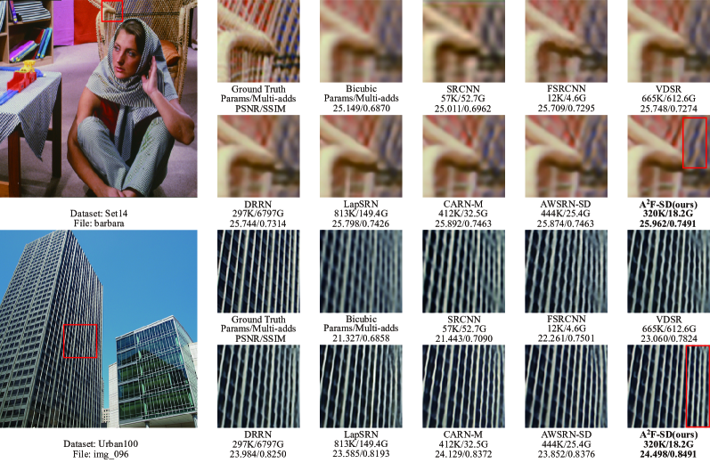
Figure 4: Qualitative comparison over datasets for scale $\times 4$. The red rectangle indicates the area of interest for zooming. Comparison for other two datasets can be seen supplementary material.

4.4.1 Qualitative comparison

Qualitative comparison is shown in Figure 4. We choose methods whose parameters are less than 1000k since we think high efficiency (low parameters) is essential. We can see that our method A²F-SD achieves better performance than others, which is represented through recovering more high-frequency information for the entire image. For the image barbara in Set14 (row 1 in Figure 4), our method performs a clear difference between the blue area and the apricot area on the right top corner of the image. Compared with AWSRN-SD which is the second method in our table, our model removes more blur and constructs more regular texture on the right top corner of the image img096 of Urban100. We own this advantage to the sufficient using of auxiliary features of previous layers which incorporate multi-scale features in different convolution progress that might contain abundant multi-frequency information. While the attention mechanism conduces to the adaptive selection of different frequency among various layers.

4.4.2 Quantitative comparison

Table 6 shows the detailed comparison results. Our models obtain a great trade-off between performance and parameters. In particular, when the number of parameters is less than 1000K, our model achieves the best result for arbitrary scales on each dataset among all of the algorithms. A²F-SD, which only has about 300K parameters, even shows better performance on a variety of datasets compared to DRCN that has nearly 1800K parameters. This proves the tremendous potential of A²F for real-world application. The high efficiency of A²F comes from the mechnism of sufficient fusion of former layers feature via the proposed attention scheme. Because we adopt 1$\times$1 Conv and channel attention to select the appropriate features of former layers for fusing, which can help to reduce the number of layers in the network without sacrificing good performance. When the number of parameters is more than 1000K, A²F-L model also performs a SOTA result on the whole, although worse in some cases slightly. It is due to that they combine all features of former layers without considering whether they are useful, which cause a reduction to performance. While compared to AWSRN-M and AWSRN, A²F-M model has more advantage in trade-off since it has comparable PSNR and SSIM but only 1010K parameters that account for 63%, 80% of AWSRN and AWSRN-M, respectively.

Table 4: Running time comparison with $\times 4$ scale on Urban100 dataset. All of them are evaluated on the same mechine.

Model	Params	Multi-Adds	Running time(s)	PSNR
RCAN [7]	15590K	919.9G	0.8746	26.82
EDSR [3]	43090K	2896.3G	0.3564	26.64
D-DBPN [21]	10430K	685.7G	0.4174	26.38
SRFBN [31]	3631K	1128.7G	0.4291	26.60
SRFBN-S [31]	483K	132.5G	0.0956	25.71
VDSR [2]	665K	612.6G	0.1165	25.18
CARN-M [32]	412K	32.5G	0.0326	25.62
A2F-SD	320K	18.2G	0.0145	25.80
A2F-L	1374K	77.2G	0.0324	26.32

4.5 Running Time and GFLOPS

We compare our model A²F-SD and A²F-L with other methods (both lightweight  [2, 31, 32] and non-lightweight [7, 3, 21]) in running time to verify the high efficiency of our work in Table 4. Like [31], we evaluate our method on a same machine with four NVIDIA 1080Ti GPUs and 3.6GHz Intel i7 CPU. All of the codes are official implementation. To be fair, we only use a single NVIDIA 1080Ti GPU for evaluation, and only contain codes that are necessary for testing an image, which means operations of saving images, saving models, opening log files, appending extra datas and so on are removed from the timing program.

To reduce the accidental error, we evaluate each method for four times on each GPU and calculate the avarage time as the final running time for a method. Table 4 shows that our models represent a significant surpass on running time for an image compared with other methods, even our A²F-L model is three times faster than SRFBN-S [31] which has only 483K parameters with 25.71 PSNR. All of our models are highly efficient and keep being less comparable with RCAN [7] which are 60 and 27 times slower than our A²F-SD, and A²F-L model, respectively. This comparison result reflects that our method gets the tremendous trade-off between performance and running time and is the best choice for realistic applications.

We also calculate the GFLOPs based on the input size of $32\times 32$ for several methods that can be comparable with A²F in Table 5. We actually get high performance with lower GFLOPs both for our large and small models.

Table 5: The perceptual metric LPIPS on five datasets for scale x4. The lower is better. We only choose methods that can be comparable with A²F. All of the output SR images are provided officially.

Methods	Params	GFLOPs	Set5	Set14	B100	Urban100	Manga109
AWSRN [28]	1587K	1.620G	0.1747	0.2853	0.3692	0.2198	0.1058
AWSRN-SD [28]	444K	-	0.1779	0.2917	0.3838	0.2468	0.1168
CARN [32]	1592K	1.620G	0.1761	0.2893	0.3799	0.2363	-
CARN-M [32]	412K	0.445G	0.1777	0.2938	0.3850	0.2524	-
SRFBN-S [31]	483K	0.323G	0.1776	0.2938	0.3861	0.2554	0.1396
IMDN [51]	715K	0.729G	0.1743	0.2901	0.3740	0.2350	0.1330
A2F-SD	320K	0.321G	0.1731	0.2870	0.3761	0.2375	0.1112
A2F-L	1374K	1.370G	0.1733	0.2846	0.3698	0.2194	0.1056

4.6 Perceptual Metric

Perceptual metric can better reflect the judgment of image quality. In this paper, LPIPS [45] is chosen as the perceptual metric. From Table 5, our proposed model obtains superior results with high efficiency in most cases, which shows their ability of generating more realistic images.

5 Conclusion

In this paper, we propose a lightweight single-image super-resolution network called A²F which adopts attentive auxiliary feature blocks to efficiently and sufficiently utilize auxiliary features. Quantitive experiment results demonstrate that auxiliary features with projection unit and channel attention can achieve higher PSNR and SSIM as well as perceptual metric LPIPS with less running time on various datasets. Qualitative experiment results reflect that auxiliary features can give the predicted image more high-frequency information, thus making the models achieve better performance. The A²F model with attentive auxiliary feature block is easy to implement and achieves great performance when the number of parameters is less than 320K and the multi-adds are less than 75G, which shows that it has great potential to be deployed in practical applications with limited computation resources. In the future, we will investigate more measures to better fuse auxiliary features.

5.0.1 Acknowledgement

This work was supported in part by the National Key Research and Development Program of China under Grant 2018YFB1305002, in part by the National Natural Science Foundation of China under Grant 61773414, and Grant 61972250, in part by the Key Research and Development Program of Guangzhou under Grant 202007050002, and Grant 202007050004.

Table 6: Evaluation on five datasets by scale $\times 2$, $\times 3$, $\times 4$. Red and blue imply the best and second best result in a group, respectively.

Scale	Size Scope	Model	Param	MutiAdds	Set5	Set14	B100	Urban100	Manga109
x2	$<5\times 10^{2}K$	FSRCNN	12K	6G	37.00/0.9558	32.63/0.9088	31.53/0.8920	29.88/0.9020	36.67/0.9694
		SRCNN	57K	52.7G	36.66/0.9542	32.42/0.9063	31.36/0.8879	29.50/0.8946	35.74/0.9661
		DRRN	297K	6797G	37.74/0.9591	33.23/0.9136	32.05/0.8973	31.23/0.9188	37.92/0.9760
		A2F-SD(ours)	313k	71.2G	37.91/0.9602	33.45/0.9164	32.08/0.8986	31.79/0.9246	38.52/0.9767
		A2F-S(ours)	320k	71.7G	37.79/0.9597	33.32/0.9152	31.99/0.8972	31.44/0.9211	38.11/0.9757
		FALSR-B	326K	74.7G	37.61/0.9585	33.29/0.9143	31.97/0.8967	31.28/0.9191	-
		AWSRN-SD	348K	79.6G	37.86/0.9600	33.41/0.9161	32.07/0.8984	31.67/0.9237	38.20/0.9762
		AWSRN-S	397K	91.2G	37.75/0.9596	33.31/0.9151	32.00/0.8974	31.39/0.9207	37.90/0.9755
		FALSR-C	408K	93.7G	37.66/0.9586	33.26/0.9140	31.96/0.8965	31.24/0.9187	-
		CARN-M	412K	91.2G	37.53/0.9583	33.26/0.9141	31.92/0.8960	31.23/0.9193	-
		SRFBN-S	483K	-	37.78/0.9597	33.35/0.9156	32.00/0.8970	31.41/0.9207	38.06/0.9757
	$<10^{3}K$	IDN	552K	-	37.83/0.9600	33.30/0.9148	32.08/0.8985	31.27/0.9196	-
		VDSR	665K	612.6G	37.53/0.9587	33.03/0.9124	31.90/0.8960	30.76/0.9140	37.22/0.9729
		MemNet	677K	2662.4G	37.78/0.9597	33.28/0.9142	32.08/0.8978	31.31/0.9195	-
		LapSRN	813K	29.9G	37.52/0.9590	33.08/0.9130	31.80/0.8950	30.41/0.9100	37.27/0.9740
		SelNet	974K	225.7G	37.89/0.9598	33.61/0.9160	32.08/0.8984	-	-
		A2F-M(ours)	999k	224.2G	38.04/0.9607	33.67/0.9184	32.18/0.8996	32.27/0.9294	38.87/0.9774
	$<2\times 10^{3}K$	FALSR-A	1021K	234.7G	37.82/0.9595	33.55/0.9168	32.12/0.8987	31.93/0.9256	-
		MoreMNAS-A	1039K	238.6G	37.63/0.9584	33.23/0.9138	31.95/0.8961	31.24/0.9187	-
		AWSRN-M	1063K	244.1G	38.04/0.9605	33.66/0.9181	32.21/0.9000	32.23/0.9294	38.66/0.9772
		A2F-L(ours)	1363k	306.1G	38.09/0.9607	33.78/0.9192	32.23/0.9002	32.46/0.9313	38.95/0.9772
		AWSRN	1397K	320.5G	38.11/0.9608	33.78/0.9189	32.26/0.9006	32.49/0.9316	38.87/0.9776
		SRMDNF	1513K	347.7G	37.79/0.9600	33.32/0.9150	32.05/0.8980	31.33/0.9200	-
		CARN	1592K	222.8G	37.76/0.9590	33.52/0.9166	32.09/0.8978	31.92/0.9256	-
		DRCN	1774K	17974G	37.63/0.9588	33.04/0.9118	31.85/0.8942	30.75/0.9133	37.63/0.9723
	$<5\times 10^{3}K$	MSRN	5930K	1365.4G	38.08/0.9607	33.70/0.9186	32.23/0.9002	32.29/0.9303	38.69/0.9772
x3	$<10^{3}K$	FSRCNN	12K	5G	33.16/0.9140	29.43/0.8242	28.53/0.7910	26.43/0.8080	30.98/0.9212
		SRCNN	57K	52.7G	32.75/0.9090	29.28/0.8209	28.41/0.7863	26.24/0.7989	30.59/0.9107
		DRRN	297K	6797G	34.03/0.9244	29.96/0.8349	28.95/0.8004	27.53/0.8378	32.74/0.9390
		A2F-SD(ours)	316k	31.9G	34.23/0.9259	30.22/0.8395	29.01/0.8028	27.91/0.8465	33.29/0.9424
		A2F-S(ours)	324k	32.3G	34.06/0.9241	30.08/0.8370	28.92/0.8006	27.57/0.8392	32.86/0.9394
		AWSRN-SD	388K	39.5G	34.18/0.9273	30.21/0.8398	28.99/0.8027	27.80/0.8444	33.13/0.9416
		CARN-M	412K	46.1G	33.99/0.9236	30.08/0.8367	28.91/0.8000	27.55/0.8385	-
		AWSRN-S	477K	48.6G	34.02/0.9240	30.09/0.8376	28.92/0.8009	27.57/0.8391	32.82/0.9393
		SRFBN-S	483K	-	34.20/0.9255	30.10/0.8372	28.96/0.8010	27.66/0.8415	33.02/0.9404
		IDN	552K	-	34.11/0.9253	29.99/0.8354	28.95/0.8013	27.42/0.8359	-
		VDSR	665K	612.6G	33.66/0.9213	29.77/0.8314	28.82/0.7976	27.14/0.8279	32.01/0.9310
		MemNet	677K	2662.4G	34.09/0.9248	30.00/0.8350	28.96/0.8001	27.56/0.8376	-
	$<2\times 10^{3}K$	A2F-M(ours)	1003k	100.0G	34.50/0.9278	30.39/0.8427	29.11/0.8054	28.28/0.8546	33.66/0.9453
		AWSRN-M	1143K	116.6G	34.42/0.9275	30.32/0.8419	29.13/0.8059	28.26/0.8545	33.64/0.9450
		SelNet	1159K	120G	34.27/0.9257	30.30/0.8399	28.97/0.8025	-	-
		A2F-L(ours)	1367k	136.3G	34.54/0.9283	30.41/0.8436	29.14/0.8062	28.40/0.8574	33.83/0.9463
		AWSRN	1476K	150.6G	34.52/0.9281	30.38/0.8426	29.16/0.8069	28.42/0.8580	33.85/0.9463
		SRMDNF	1530K	156.3G	34.12/0.9250	30.04/0.8370	28.97/0.8030	27.57/0.8400	-
		CARN	1592K	118.8G	34.29/0.9255	30.29/0.8407	29.06/0.8034	28.06/0.8493	-
		DRCN	1774K	17974G	33.82/0.9226	29.76/0.8311	28.80/0.7963	27.15/0.8276	32.31/0.9328
	$<10^{4}K$	MSRN	6114K	625.7G	34.46/0.9278	30.41/0.8437	29.15/0.8064	28.33/0.8561	33.67/0.9456
x4	$<10^{3}K$	FSRCNN	12K	4.6G	30.71/0.8657	27.59/0.7535	26.98/0.7150	24.62/0.7280	27.90/0.8517
		SRCNN	57K	52.7G	30.48/0.8628	27.49/0.7503	26.90/0.7101	24.52/0.7221	27.66/0.8505
		DRRN	297K	6797G	31.68/0.8888	28.21/0.7720	27.38/0.7284	25.44/0.7638	29.46/0.8960
		A2F-SD(ours)	320k	18.2G	32.06/0.8928	28.47/0.7790	27.48/0.7373	25.80/0.7767	30.16/0.9038
		A2F-S(ours)	331k	18.6G	31.87/0.8900	28.36/0.7760	27.41/0.7305	25.58/0.7685	29.77/0.8987
		CARN-M	412K	32.5G	31.92/0.8903	28.42/0.7762	27.44/0.7304	25.62/0.7694	-
		AWSRN-SD	444K	25.4G	31.98/0.8921	28.46/0.7786	27.48/0.7368	25.74/0.7746	30.09/0.9024
		SRFBN-S	483K	132.5G	31.98/0.8923	28.45/0.7779	27.44/0.7313	25.71/0.7719	29.91/0.9008
		IDN	552K	-	31.82/0.8903	28.25/0.7730	27.41/0.7297	25.41/0.7632	-
		AWSRN-S	588K	37.7G	31.77/0.8893	28.35/0.7761	27.41/0.7304	25.56/0.7678	29.74/0.8982
		VDSR	665K	612.6G	31.35/0.8838	28.01/0.7674	27.29/0.7251	25.18/0.7524	28.83/0.8809
		MemNet	677K	2662.4G	31.74/0.8893	28.26/0.7723	27.40/0.7281	25.50/0.7630	-
		LapSRN	813K	149.4G	31.54/0.8850	28.19/0.7720	27.32/0.7280	25.21/0.7560	29.09/0.8845
	$<2\times 10^{3}K$	A2F-M(ours)	1010k	56.7G	32.28/0.8955	28.62/0.7828	27.58/0.7364	26.17/0.7892	30.57/0.9100
		AWSRN-M	1254K	72G	32.21/0.8954	28.65/0.7832	27.60/0.7368	26.15/0.7884	30.56/0.9093
		A2F-L(ours)	1374K	77.2G	32.32/0.8964	28.67/0.7839	27.62/0.7379	26.32/0.7931	30.72/0.9115
		SelNet	1417K	83.1G	32.00/0.8931	28.49/0.7783	27.44/0.7325	-	-
		SRMDNF	1555K	89.3G	31.96/0.8930	28.35/0.7770	27.49/0.7340	25.68/0.7730	-
		AWSRN	1587K	91.1G	32.27/0.8960	28.69/0.7843	27.64/0.7385	26.29/0.7930	30.72/0.9109
		CARN	1592K	90.9G	32.13/0.8937	28.60/0.7806	27.58/0.7349	26.07/0.7837	-
		DRCN	1774K	17974G	31.53/0.8854	28.02/0.7670	27.23/0.7233	25.14/0.7510	28.98/0.8816
	$<10^{4}K$	SRDenseNet	2015K	389.9K	32.02/0.8934	28.35/0.7770	27.53/0.7337	26.05/0.7819	-
		MSRN	6078K	349.8G	32.26/0.8960	28.63/0.7836	27.61/0.7380	26.22/0.7911	30.57/0.9103

References

- [1] Dong, C., Loy, C.C., He, K., Tang, X.: Image super-resolution using deep convolutional networks. IEEE transactions on pattern analysis and machine intelligence 38 (2015) 295–307
- [2] Kim, J., Kwon Lee, J., Mu Lee, K.: Accurate image super-resolution using very deep convolutional networks. In: Proceedings of the IEEE conference on computer vision and pattern recognition. (2016) 1646–1654
- [3] Lim, B., Son, S., Kim, H., Nah, S., Mu Lee, K.: Enhanced deep residual networks for single image super-resolution. In: Proceedings of the IEEE conference on computer vision and pattern recognition workshops. (2017) 136–144
- [4] Tong, T., Li, G., Liu, X., Gao, Q.: Image super-resolution using dense skip connections. In: Proceedings of the IEEE International Conference on Computer Vision. (2017) 4799–4807
- [5] Yu, J., Fan, Y., Yang, J., Xu, N., Wang, Z., Wang, X., Huang, T.: Wide activation for efficient and accurate image super-resolution. arXiv preprint arXiv:1808.08718 (2018)
- [6] Zhang, K., Wang, B., Zuo, W., Zhang, H., Zhang, L.: Joint learning of multiple regressors for single image super-resolution. IEEE Signal processing letters 23 (2015) 102–106
- [7] Zhang, Y., Li, K., Li, K., Wang, L., Zhong, B., Fu, Y.: Image super-resolution using very deep residual channel attention networks. In: Proceedings of the European Conference on Computer Vision (ECCV). (2018) 286–301
- [8] Chen, L., Zhan, W., Tian, W., He, Y., Zou, Q.: Deep integration: A multi-label architecture for road scene recognition. IEEE Transactions on Image Processing (2019)
- [9] Hsiao, P.H., Chang, P.L.: Video enhancement via super-resolution using deep quality transfer network. In: Asian Conference on Computer Vision, Springer (2016) 184–200
- [10] Peled, S., Yeshurun, Y.: Superresolution in mri: application to human white matter fiber tract visualization by diffusion tensor imaging. Magnetic Resonance in Medicine: An Official Journal of the International Society for Magnetic Resonance in Medicine 45 (2001) 29–35
- [11] Shi, W., Caballero, J., Ledig, C., Zhuang, X., Bai, W., Bhatia, K., de Marvao, A.M.S.M., Dawes, T., O’Regan, D., Rueckert, D.: Cardiac image super-resolution with global correspondence using multi-atlas patchmatch. In: International Conference on Medical Image Computing and Computer-Assisted Intervention, Springer (2013) 9–16
- [12] Valmadre, J., Bertinetto, L., Henriques, J., Vedaldi, A., Torr, P.H.: End-to-end representation learning for correlation filter based tracking. In: Proceedings of the IEEE Conference on Computer Vision and Pattern Recognition. (2017) 2805–2813
- [13] Zhang, L., Zhang, H., Shen, H., Li, P.: A super-resolution reconstruction algorithm for surveillance images. Signal Processing 90 (2010) 848–859
- [14] Yang, X., Yan, J.: Arbitrary-oriented object detection with circular smooth label. In: Proceedings of the Europeon Conference on Computer Vision. (2020)
- [15] Chen, L., Zou, Q., Pan, Z., Lai, D., Zhu, L., Hou, Z., Wang, J., Cao, D.: Surrounding vehicle detection using an fpga panoramic camera and deep cnns. IEEE Transactions on Intelligent Transportation Systems (2019)
- [16] Shen, W., Guo, Y., Wang, Y., Zhao, K., Wang, B., Yuille, A.L.: Deep differentiable random forests for age estimation. IEEE transactions on pattern analysis and machine intelligence (2019)
- [17] Yang, X., Yang, J., Yan, J., Zhang, Y., Zhang, T., Guo, Z., Sun, X., Fu, K.: Scrdet: Towards more robust detection for small, cluttered and rotated objects. In: Proceedings of the IEEE International Conference on Computer Vision. (2019) 8232–8241
- [18] Chen, L., Wang, Q., Lu, X., Cao, D., Wang, F.Y.: Learning driving models from parallel end-to-end driving data set. Proceedings of the IEEE 108 (2019) 262–273
- [19] Matsui, Y., Ito, K., Aramaki, Y., Fujimoto, A., Ogawa, T., Yamasaki, T., Aizawa, K.: Sketch-based manga retrieval using manga109 dataset. Multimedia Tools and Applications 76 (2017) 21811–21838
- [20] Li, J., Fang, F., Mei, K., Zhang, G.: Multi-scale residual network for image super-resolution. In: Proceedings of the European Conference on Computer Vision (ECCV). (2018) 517–532
- [21] Haris, M., Shakhnarovich, G., Ukita, N.: Deep back-projection networks for super-resolution. In: Proceedings of the IEEE conference on computer vision and pattern recognition. (2018) 1664–1673
- [22] Dong, C., Loy, C.C., Tang, X.: Accelerating the super-resolution convolutional neural network. In: European conference on computer vision, Springer (2016) 391–407
- [23] Kim, J., Kwon Lee, J., Mu Lee, K.: Deeply-recursive convolutional network for image super-resolution. In: Proceedings of the IEEE conference on computer vision and pattern recognition. (2016) 1637–1645
- [24] Shi, W., Caballero, J., Huszár, F., Totz, J., Aitken, A.P., Bishop, R., Rueckert, D., Wang, Z.: Real-time single image and video super-resolution using an efficient sub-pixel convolutional neural network. In: Proceedings of the IEEE conference on computer vision and pattern recognition. (2016) 1874–1883
- [25] Tai, Y., Yang, J., Liu, X.: Image super-resolution via deep recursive residual network. In: Proceedings of the IEEE conference on computer vision and pattern recognition. (2017) 3147–3155
- [26] Chu, X., Zhang, B., Ma, H., Xu, R., Li, J., Li, Q.: Fast, accurate and lightweight super-resolution with neural architecture search. arXiv preprint arXiv:1901.07261 (2019)
- [27] Chu, X., Zhang, B., Xu, R., Ma, H.: Multi-objective reinforced evolution in mobile neural architecture search. arXiv preprint arXiv:1901.01074 (2019)
- [28] Wang, C., Li, Z., Shi, J.: Lightweight image super-resolution with adaptive weighted learning network. arXiv preprint arXiv:1904.02358 (2019)
- [29] Zhao, X., Liao, Y., Lfi, Y., Zhang, T., Zou, X.: Fc2n: Fully channel-concatenated network for single image super-resolution. arXiv preprint arXiv:1907.03221 (2019)
- [30] Shi, W., Caballero, J., Huszár, F., Totz, J., Aitken, A.P., Bishop, R., Rueckert, D., Wang, Z.: Real-time single image and video super-resolution using an efficient sub-pixel convolutional neural network. In: Proceedings of the IEEE conference on computer vision and pattern recognition. (2016) 1874–1883
- [31] Li, Z., Yang, J., Liu, Z., Yang, X., Jeon, G., Wu, W.: Feedback network for image super-resolution. In: Proceedings of the IEEE Conference on Computer Vision and Pattern Recognition. (2019) 3867–3876
- [32] Ahn, N., Kang, B., Sohn, K.A.: Fast, accurate, and lightweight super-resolution with cascading residual network. In: Proceedings of the European Conference on Computer Vision (ECCV). (2018) 252–268
- [33] He, K., Zhang, X., Ren, S., Sun, J.: Deep residual learning for image recognition. In: Proceedings of the IEEE conference on computer vision and pattern recognition. (2016) 770–778
- [34] Huang, G., Liu, Z., Van Der Maaten, L., Weinberger, K.Q.: Densely connected convolutional networks. In: Proceedings of the IEEE conference on computer vision and pattern recognition. (2017) 4700–4708
- [35] Tai, Y., Yang, J., Liu, X., Xu, C.: Memnet: A persistent memory network for image restoration. In: Proceedings of the IEEE international conference on computer vision. (2017) 4539–4547
- [36] Zhang, Y., Tian, Y., Kong, Y., Zhong, B., Fu, Y.: Residual dense network for image super-resolution. In: Proceedings of the IEEE Conference on Computer Vision and Pattern Recognition. (2018) 2472–2481
- [37] Bahdanau, D., Cho, K., Bengio, Y.: Neural machine translation by jointly learning to align and translate. arXiv preprint arXiv:1409.0473 (2014)
- [38] Hu, J., Shen, L., Sun, G.: Squeeze-and-excitation networks. In: Proceedings of the IEEE conference on computer vision and pattern recognition. (2018) 7132–7141
- [39] Agustsson, E., Timofte, R.: Ntire 2017 challenge on single image super-resolution: Dataset and study. In: The IEEE Conference on Computer Vision and Pattern Recognition (CVPR) Workshops. (2017)
- [40] Wang, Z., Bovik, A.C., Sheikh, H.R., Simoncelli, E.P.: Image quality assessment: from error visibility to structural similarity. IEEE transactions on image processing 13 (2004) 600–612
- [41] Bevilacqua, M., Roumy, A., Guillemot, C., Alberi-Morel, M.L.: Low-complexity single-image super-resolution based on nonnegative neighbor embedding. (2012)
- [42] Yang, J., Wright, J., Huang, T.S., Ma, Y.: Image super-resolution via sparse representation. IEEE transactions on image processing 19 (2010) 2861–2873
- [43] Martin, D., Fowlkes, C., Tal, D., Malik, J., et al.: A database of human segmented natural images and its application to evaluating segmentation algorithms and measuring ecological statistics, Iccv Vancouver: (2001)
- [44] Huang, J.B., Singh, A., Ahuja, N.: Single image super-resolution from transformed self-exemplars. In: Proceedings of the IEEE Conference on Computer Vision and Pattern Recognition. (2015) 5197–5206
- [45] Zhang, R., Isola, P., Efros, A.A., Shechtman, E., Wang., O.: The unreasonable effectiveness of deep features as a perceptual metric. In: Proceedings of the IEEE conference on computer vision and pattern recognition. (2018)
- [46] Kingma, D.P., Ba, J.: Adam: A method for stochastic optimization. arXiv preprint arXiv:1412.6980 (2014)
- [47] Lai, W.S., Huang, J.B., Ahuja, N., Yang, M.H.: Deep laplacian pyramid networks for fast and accurate super-resolution. In: Proceedings of the IEEE conference on computer vision and pattern recognition. (2017) 624–632
- [48] Zhang, K., Zuo, W., Zhang, L.: Learning a single convolutional super-resolution network for multiple degradations. In: Proceedings of the IEEE Conference on Computer Vision and Pattern Recognition. (2018) 3262–3271
- [49] Choi, J.S., Kim, M.: A deep convolutional neural network with selection units for super-resolution. In: Proceedings of the IEEE Conference on Computer Vision and Pattern Recognition Workshops. (2017) 154–160
- [50] Hui, Z., Wang, X., Gao, X.: Fast and accurate single image super-resolution via information distillation network. In: Proceedings of the IEEE conference on computer vision and pattern recognition. (2018) 723–731
- [51] Hui, Z., Gao, X., Yang, Y., Wang, X.: Lightweight image super-resolution with information multidistillation network. In: ACM Multimedia. (2019)