When Should We (Not) Interpret Linear IV Estimands as LATE?

In this paper I revisit the interpretation of the linear instrumental variables (IV) estimand as a weighted average of conditional local average treatment effects (LATEs). I focus on a practically relevant situation in which additional covariates are required for identification while the reduced-form and first-stage regressions implicitly restrict the effects of the instrument to be homogeneous, and are thus possibly misspecified. I show that the weights on some conditional LATEs are negative and the IV estimand is no longer interpretable as a causal effect under a weaker version of monotonicity, i.e. when there are compliers but no defiers at some covariate values and defiers but no compliers elsewhere. The problem of negative weights disappears in the overidentified specification of Angrist and Imbens (1995) and in an alternative method, termed “reordered IV,” that I also outline. Even if all weights are positive, the IV estimand in the just identified specification is not interpretable as the unconditional LATE parameter unless the groups with different values of the instrument are roughly equal sized. I illustrate my findings in an application to causal effects of college education using the college proximity instrument. The benchmark estimates suggest that college attendance yields earnings gains of about 60 log points, which is well outside the range of estimates in the recent literature. I demonstrate, however, that this result is driven by the presence of negative weights. Corrected estimates indicate that attending college causes earnings to be roughly 20% higher.

1 Introduction

Many instrumental variables are only valid after conditioning on additional covariates. The draft eligibility instrument in Angrist (1990) requires controlling for year of birth. The college proximity instrument in Card (1995) is invalid without conditioning on a number of individual characteristics of workers (Kitagawa, 2015). Even in the case of randomized experiments with noncompliance, it is often necessary to control for covariates that are correlated with treatment probability, such as household size and survey wave in Finkelstein et al. (2012).

When conditioning on additional covariates is necessary for instrument validity, the interpretation of the linear instrumental variables (IV) and two-stage least squares (2SLS) estimands becomes tricky. Angrist and Imbens (1995) provide an influential interpretation of the 2SLS estimand in this context as a convex combination of conditional local average treatment effects (LATEs), i.e. average effects of treatment for individuals whose treatment status is affected by the instrument. This result, however, is restricted to saturated models with discrete covariates and first-stage regressions that include a full set of interactions between these covariates and the instrument; this is equivalent to requiring that the researcher estimates a separate first stage for every combination of covariate values. Such specifications are very rare in empirical work, as is evident from several recent surveys of applications of IV methods. This severely limits the applicability of Angrist and Imbens (1995)’s result to interpreting actual IV and 2SLS estimates (cf. Abadie, 2003).

In an important contribution, Kolesár (2013) relaxes many of the limitations of Angrist and Imbens (1995)’s result and supports the view that linear IV and 2SLS estimands can generally be written as a convex combination of conditional LATEs. Kolesár (2013)’s result allows for misspecification of the first stage as well as what I refer to as “weak monotonicity,” i.e. the existence of compliers but no defiers at some covariate values and the existence of defiers but no compliers elsewhere. Kolesár (2013) concludes that even in this case the interpretation of linear IV and 2SLS estimands as a convex combination of conditional LATEs is generally correct, subject to some additional assumptions. These assumptions essentially require that the first stage postulated by the researcher provides a sufficiently good approximation to the true first stage.

In this paper I present a more pessimistic view of the causal interpretability of linear IV and 2SLS estimands. In particular, I study the questions of whether the IV weights on conditional LATEs are positive and, if they are, whether they have an intuitive interpretation. My answer to both of these questions is rather negative. To be specific, I make four contributions to the literature on instrumental variables. First, I demonstrate that under weak monotonicity the weights on some conditional LATEs are negative in the common situation where the first stage incorrectly restricts the effects of the instrument to be homogeneous. While Kolesár (2013)’s results apply to a wide range of specifications, his conditions for positive weights are not satisfied in this benchmark case. It follows that the IV estimand may no longer be interpretable as a causal effect; this parameter may turn out to be negative (positive) even if treatment effects are positive (negative) for everyone in the population.

Second, unlike in previous contributions to this literature, I explicitly compare the weights in the usual application of IV and in Angrist and Imbens (1995)’s specification with what I refer to as the “desired” weights, that is, the weights that recover the unconditional LATE parameter. The advantage of Angrist and Imbens (1995)’s specification is that it is guaranteed to produce a convex combination of conditional LATEs even under weak monotonicity. However, if the existence of defiers is ruled out at all covariate values, which I refer to as “strong monotonicity,” both specifications overweight the effects in groups with large variances of the instrument while Angrist and Imbens (1995)’s specification also overweights the effects in groups with strong first stages. This additional difference between the “desired” weights and Angrist and Imbens (1995)’s weights could make the usual application of IV more suitable under strong monotonicity.

Third, I outline a simple diagnostic for negative weights and an alternative estimation method, which shares the ability of Angrist and Imbens (1995)’s specification to deliver a convex combination of conditional LATEs. In particular, I recommend that empirical researchers begin their analysis by estimating the first stage in a flexible way, allowing for heterogeneous effects of the instrument. A testable implication of strong monotonicity is that the sign of the first stage is the same for all covariate values. If this requirement is not satisfied, which is easy to verify, the usual application of IV will not be valid. Alternatively, the first-stage estimates can be used to “reorder” the values of the instrument. Indeed, we can redefine the instrument to take the value 1 for this value of the original instrument that encourages treatment conditional on covariates and the value 0 otherwise. This new instrument can then be used in a just identified specification, which I refer to as “reordered IV” and where the weights on all conditional LATEs are again positive.

Finally, I demonstrate that the weights in the standard (just identified) specification are potentially problematic for the casual interpretation of the IV estimand as “the LATE” even under strong monotonicity. Specifically, I show that if the groups with different values of the instrument are not approximately equal sized, the IV estimand may be quantitatively and qualitatively different from the unconditional LATE parameter, which is how the term “the LATE,” as used in empirical work, should presumably be understood. In other words, I demonstrate that the IV estimand may be substantially different from the usual parameter of interest even if all weights are positive and integrate to one, unless the relevant population is balanced in a particular sense. I develop simple diagnostic tools to detect whether the otherwise positive weights are problematic or not.

While these diagnostics are helpful in identifying situations where the IV estimand may not correspond to an interesting target parameter, whether the two objects differ in a meaningful way is ultimately an empirical question. Thus, the simplest takeaway from this paper is as follows. Empirical researchers with a preference for linear IV should supplement each of their specifications with two alternative estimates. The first would be based either on the overidentified specification of Angrist and Imbens (1995), perhaps estimated using the unbiased jackknife IV estimator (UJIVE) of Kolesár (2013), or the “reordered IV” procedure of this paper. The second would use any flexible estimator of the unconditional LATE parameter, such as those in Tan (2006), Frölich (2007), Hong and Nekipelov (2010), Donald et al. (2014), Sant’Anna et al. (2021), and Słoczyński et al. (2022). In the absence of substantial problems with weak instruments, the resulting three estimates should be similar, unless some of the IV weights are negative or they are all positive but do not recover the unconditional LATE parameter anyway.

I conclude this paper with a replication of Card (1995)’s analysis of returns to schooling using the college proximity instrument. Focusing on causal effects of college education, I show that the benchmark estimates suggest that college attendance yields earnings gains of about 60 log points, which substantially exceeds the range of estimates in the recent literature (e.g., Hoekstra, 2009; Zimmerman, 2014; Smith et al., 2020). Then, however, I demonstrate that this result is driven by the presence of negative weights. Corrected estimates, including nonparametric estimates of the unconditional LATE parameter, indicate that attending college causes earnings to be about 20% higher, which is in line with the recent empirical literature.

In a related contribution, released after this paper first circulated, Blandhol et al. (2022) offer another pessimistic view of the causal interpretability of linear IV and 2SLS estimands. Unlike this paper, Blandhol et al. (2022) focus on the consequences of misspecification of the model for the instrument propensity score that is implicit in IV and 2SLS estimation. Both papers discuss the consequences of violations of strong monotonicity. Unlike Blandhol et al. (2022), I also study potential problems with the IV estimand in the case where all weights are positive. This scenario would often be regarded as optimistic and I argue that this is not necessarily the case. Ruling out the existence of negative weights is necessary but not sufficient for an estimand to correspond to an interesting target parameter (cf. Callaway et al., 2021; Callaway and Sant’Anna, 2021).

The remainder of the paper is organized as follows. Section 2 introduces my framework. Section 3 studies the question of whether linear IV and 2SLS estimands can generally be written as a convex combination of conditional LATEs. Section 4 demonstrates that the IV weights may continue to be problematic even in cases where they are positive. Section 5 illustrates my findings in an application to causal effects of college education. Section 6 concludes.

2 Framework

In this section I formally define the statistical objects of interest, i.e. the conditional and unconditional IV and 2SLS estimands. I reserve the term “2SLS” for the appropriate estimator and estimand in overidentified models; see equation (3) below. When the model is just identified, I use the term “IV” or “linear IV”; see equation (2). In what follows, I also review identification in the LATE framework with covariates (see, e.g., Abadie, 2003; Frölich, 2007). Unlike in most previous studies, I devote particular attention to the possibility that compliers and defiers may coexist but not at any given value of covariates (see also Kolesár, 2013; Semenova, 2021). Throughout the paper I also assume that the appropriate moments exist whenever necessary.

2.1 Notation and Estimands

Suppose that we are interested in the causal effect of a binary treatment, $D$, on an outcome, $Y$. For every individual, we define two potential outcomes, $Y(1)$ and $Y(0)$, which correspond to the values of $Y$ that this individual would attain if treated ($D=1$) and if not treated ($D=0$), respectively. Thus, $Y(1)-Y(0)$ is the treatment effect. The treatment $D$ is allowed to be endogenous but a binary instrument, $Z$, is also available. Let $D(1)$ and $D(0)$ denote the potential treatment statuses that correspond to the treatment actually received by an individual when their instrument assignment is given by $Z=1$ and $Z=0$, respectively. Consequently, $Y=Y(D)$ and $D=D(Z)$. If the observed outcome were to depend directly on $Z$, we would write $Y=Y(Z,D)$. Finally, let $X=\left(1,X_{1},\ldots,X_{J}\right)$ denote a row vector of covariates. In some cases I will allow for the possibility that additional instruments have been created by interacting $Z$ with all elements of $X$; then, $Z_{\mathrm{C}}=\left(Z,ZX_{1},\ldots,ZX_{J}\right)$ will be used to denote the resulting row vector of instruments.

To provide motivation for what follows, let us consider the standard single-equation linear model for our outcome of interest:

$$Y=D\beta+X\gamma+\upsilon,$$ (1)

where $X$ and the instrument(s) are assumed to be uncorrelated with $\upsilon$. Also, $\beta$ is the coefficient of interest. Unlike in textbook treatments of this model but in line with the literature on local average treatment effects, I do not assume that equation (1) is correctly specified; in particular, I allow the effect of $D$ on $Y$ to be heterogeneous and correlated with both observables and unobservables.

In practice, however, many researchers act as if this model is correctly specified and use linear IV or 2SLS for estimation. In what follows, I will focus on the interpretation of the probability limits of the IV and 2SLS estimators of $\beta$ when equation (1) is possibly misspecified. With a single instrument, the probability limit of linear IV or, simply, the (linear) IV estimand is

$$\beta_{\mathrm{IV}}=\left[\left(\mathrm{E}\left[Q^{\prime}W\right]\right)^{-1}\mathrm{E}\left[Q^{\prime}Y\right]\right]_{1},$$ (2)

where $W=\left(D,X\right)$, $Q=\left(Z,X\right)$, and $\left[\cdot\right]_{k}$ denotes the $k$th element of the corresponding vector. It is useful to note that equation (2) characterizes the usual (just identified) application of instrumental variables when a single instrument is available. This specification also corresponds to reduced-form and first-stage regressions that project $Y$ and $D$, respectively, on $X$ and $Z$, excluding any interactions between $X$ and $Z$.

If a vector of instruments, $Z_{\mathrm{C}}$, has been created and 2SLS is used for estimation, the relevant probability limit or, simply, the 2SLS estimand is

$$\beta_{\mathrm{2SLS}}=\left[\left(\mathrm{E}\left[W^{\prime}Q_{\mathrm{C}}\right]\left(\mathrm{E}\left[Q_{\mathrm{C}}^{\prime}Q_{\mathrm{C}}\right]\right)^{-1}\mathrm{E}\left[Q_{\mathrm{C}}^{\prime}W\right]\right)^{-1}\mathrm{E}\left[W^{\prime}Q_{\mathrm{C}}\right]\left(\mathrm{E}\left[Q_{\mathrm{C}}^{\prime}Q_{\mathrm{C}}\right]\right)^{-1}\mathrm{E}\left[Q_{\mathrm{C}}^{\prime}Y\right]\right]_{1},$$ (3)

where $Q_{\mathrm{C}}=\left(Z_{\mathrm{C}},X\right)$. In this specification, the corresponding reduced-form and first-stage regressions project $Y$ and $D$, respectively, on $X$ and $Z_{\mathrm{C}}$, and hence we implicitly allow for heterogeneity in the effects of $Z$ on $Y$ and $D$.

Regardless of the implicit restrictions on the effects of the instrument, the true first stage can be written as

$$\mathrm{E}\left[D\mid X,Z\right]=\psi(X)+\omega(X)\cdot Z,$$ (4)

where

$$\omega(x)=\mathrm{E}\left[D\mid Z=1,X=x\right]-\mathrm{E}\left[D\mid Z=0,X=x\right]$$ (5)

is the conditional first-stage slope coefficient or, equivalently, the coefficient on $Z$ in the regression of $D$ on $1$ and $Z$ in the subpopulation with $X=x$. Similarly, the conditional IV (or Wald) estimand can be written as

$$\beta(x)=\frac{\mathrm{E}\left[Y\mid Z=1,X=x\right]-\mathrm{E}\left[Y\mid Z=0,X=x\right]}{\mathrm{E}\left[D\mid Z=1,X=x\right]-\mathrm{E}\left[D\mid Z=0,X=x\right]}.$$ (6)

This parameter is equivalent to the coefficient on $D$ in the IV regression of $Y$ on $1$ and $D$ in the subpopulation with $X=x$, with $Z$ as the instrument for $D$.

2.2 Local Average Treatment Effects

In what follows, I will briefly review the LATE framework of Imbens and Angrist (1994) and Angrist et al. (1996), focusing on its extension to the case with additional covariates.

The population consists of four latent groups: always-takers, for whom $D(1)=1$ and $D(0)=1$; never-takers, for whom $D(1)=0$ and $D(0)=0$; compliers, for whom $D(1)=1$ and $D(0)=0$; and defiers, for whom $D(1)=0$ and $D(0)=1$. As demonstrated by Imbens and Angrist (1994), if, among other things, we rule out the existence of defiers and assume that $X$ is orthogonal to $Z$, the estimand of interest, $\beta_{\mathrm{IV}}=\beta_{\mathrm{2SLS}}=\frac{\mathrm{E}\left[Y\mid Z=1\right]-\mathrm{E}\left[Y\mid Z=0\right]}{\mathrm{E}\left[D\mid Z=1\right]-\mathrm{E}\left[D\mid Z=0\right]}$, recovers the average treatment effect for compliers, usually referred to as the local average treatment effect (LATE).

Some of my results will allow for the existence of both compliers and defiers, and hence throughout this paper I follow Kolesár (2013) in defining LATE as

$$\tau_{\mathrm{LATE}}=\mathrm{E}\left[Y(1)-Y(0)\mid D(1)\neq D(0)\right],$$ (7)

i.e. the average treatment effect for individuals whose treatment status is affected by the instrument. This group includes both compliers and defiers; it will be restricted to compliers whenever the existence of defiers is ruled out. It is useful to note that this unconditional LATE parameter can also be written as

$$\tau_{\mathrm{LATE}}=\frac{\mathrm{E}\left[\pi(X)\cdot\tau(X)\right]}{\mathrm{E}\left[\pi(X)\right]},$$ (8)

where

$$\tau(x)=\mathrm{E}\left[Y(1)-Y(0)\mid D(1)\neq D(0),X=x\right]$$ (9)

is the conditional LATE and

$$\pi(x)=\mathrm{P}\left[D(1)\neq D(0)\mid X=x\right]$$ (10)

is the conditional proportion of compliers and defiers. The following assumption, together with additional assumptions below, will be used to identify $\tau(x)$ and $\pi(x)$, and thereby also $\tau_{\mathrm{LATE}}$.

Assumption IV.

2. (Conditional independence)   $\big{(}Y(0,0),Y(0,1),Y(1,0),Y(1,1),D(0),D(1)\big{)}\perp Z\mid X$;

3. (Exclusion restriction)   $\mathrm{P}\left[Y(1,d)=Y(0,d)\mid X\right]=1$ for $d\in\{0,1\}$ a.s.;

4. (Relevance)   $0<\mathrm{P}\left[Z=1\mid X\right]<1$ and $\mathrm{P}\left[D(1)=1\mid X\right]\neq\mathrm{P}\left[D(0)=1\mid X\right]$ a.s.

Assumption IV(i) postulates that the instrument is “as good as randomly assigned” conditional on covariates. Assumption IV(ii) states that the instrument does not directly affect the outcome; its only effect on the outcome is through treatment status. Finally, Assumption IV(iii) requires that there is variation in the instrument as well as a distinct number of compliers and defiers at every value of covariates, that is, the instrument is relevant. I do not assume that $X$ is orthogonal to $Z$.

Assumption IV is not sufficient to identify $\tau(x)$ and $\pi(x)$. It is also necessary to restrict the existence of defiers (Imbens and Angrist, 1994). The following assumption, due to Abadie (2003), rules out the existence of defiers at any value of covariates.

Assumption SM (Strong monotonicity).

$\mathrm{P}\left[D(1)\geq D(0)\mid X\right]=1$ a.s.

In many applications, Assumption SM may be too restrictive (cf. de Chaisemartin, 2017; Dahl et al., 2019). A testable implication of Assumption SM is that $\omega(x)$, the conditional first-stage slope coefficient, is always nonnegative. If this implication is rejected, an alternative assumption is necessary to obtain point identification. One possibility is to restrict treatment effect heterogeneity, as discussed by Heckman and Vytlacil (2005) and Mogstad and Torgovitsky (2018), in which case we will be able to identify the average treatment effect rather than the unconditional LATE parameter. Another possibility is to replace Assumption SM with a weaker assumption that postulates the existence of compliers but no defiers at some covariate values and the existence of defiers but no compliers elsewhere (cf. Kolesár, 2013; Semenova, 2021). While the relative appeal of these two assumptions is context dependent, I will mostly focus on the latter in what follows.

Assumption WM (Weak monotonicity).

There exists a partition of the covariate space such that $\mathrm{P}\left[D(1)\geq D(0)\mid X\right]=1$ a.s. on one subset and $\mathrm{P}\left[D(1)\leq D(0)\mid X\right]=1$ a.s. on its complement.

To understand the difference between Assumptions SM and WM, consider a recent paper by Deryugina et al. (2019), who estimate the health effects of air pollution using an instrument based on changes in local wind direction. Imagine a pollution source located to the east of a particular city. When the wind also blows from the east, the city will experience relatively high levels of pollution; the opposite is true when the wind blows from the west. Assumption SM would require that every city reacts to a specific wind direction (say, east) in the same way (say, high pollution). This, however, is known not to be true. Deryugina et al. (2019) explain, for example, that air pollution is relatively high in San Francisco when the wind blows from the southeast, while the same is true in Boston when the wind blows from the southwest. Indeed, Assumption WM would allow for the possibility that different locations react to a specific wind direction in different ways.

Alternatively, consider an application of the “judges design” in Maestas et al. (2013), who study the effects of disability insurance receipt on labor supply using plausibly random variation in strictness of disability examiners. In a simple setting with two examiners, Assumption SM would require that one examiner is universally more lenient than the other, which may not be reasonable. On the other hand, Assumption WM would allow for the possibility that, say, one examiner is more lenient towards male applicants and the other towards female applicants. Or, they may differ in their treatment of applicants with specific types of impairments, such as mental health and musculoskeletal conditions (cf. Maestas et al., 2013; Autor et al., 2019). It seems reasonable to allow for such a possibility, and this is indeed acknowledged in a growing number of papers in this literature (see also Frandsen et al., 2019).

Even though Assumption WM is weaker than Assumption SM, in some contexts it is still fairly strong. While it allows compliers and defiers to coexist, it postulates that the sign of the effect of $Z$ on $D$ depends only on observable characteristics. For example, many papers use the distance to the nearest college as an instrument for educational attainment, with the notion that college proximity decreases the cost and thereby encourages college attendance (e.g., Card, 1995). However, Frölich and Sperlich (2019) argue that some students may be encouraged to attend college if the nearest college is far away, as this gives them an excuse to move out of the parental home. Given that this is unlikely to affect students with binding financial constraints, it is conceivable that college proximity never discourages poor students from attending college and never encourages rich students to do so. This would be consistent with Assumption WM. In contrast, Assumption SM requires that there are no students at any value of covariates who act according to Frölich and Sperlich (2019)’s mechanism or “defy” their instrument assignment for any other reason. While it is thus obviously true that Assumption WM is weaker than Assumption SM, it is still restrictive to assume that all rich students and all poor students are affected by college proximity in the same direction (if at all), even if the direction itself is allowed to be different for the two groups.

In any case, Assumption WM may constitute a useful way forward when Assumption SM is rejected and the researcher is unwilling to restrict treatment effect heterogeneity or give up point identification. Indeed, Assumption WM, together with Assumption IV, still allows us to identify $\tau(x)$ and $\pi(x)$. Before stating the relevant lemma, it is useful to define an auxiliary function

$$c(x)=\mathrm{sgn}\Big{(}\mathrm{P}\left[D(1)\geq D(0)\mid X=x\right]-\mathrm{P}\left[D(1)\leq D(0)\mid X=x\right]\Big{)},$$ (11)

where $\mathrm{sgn}(\cdot)$ is the sign function. Clearly, $c(x)$ equals 1 if there are only compliers at $X=x$ and $-1$ if there are only defiers at $X=x$.

The following lemma summarizes identification of the conditional LATE parameter and the conditional proportion of individuals whose treatment status is affected by the instrument.

Lemma 2.1.

2. Under Assumptions IV and SM, $\tau(x)=\beta(x)$ and $\pi(x)=\omega(x)$.

3. Under Assumptions IV and WM, $\tau(x)=\beta(x)$ and $\pi(x)=\left\lvert\omega(x)\right\rvert=c(x)\cdot\omega(x)$.

Lemma 2.1 consists of well-known results and straightforward extensions of these results, and as such it is stated without proof (cf. Angrist et al., 1996; Angrist and Pischke, 2009). The conditional Wald estimand identifies the conditional LATE parameter under both strong and weak monotonicity. Under Assumption SM, the conditional proportion of compliers is identified as the conditional first-stage slope coefficient, $\omega(x)$. Under Assumption WM, the conditional proportion of compliers or defiers is identified as the absolute value of this coefficient; the coefficient is negative if and only if there are defiers but no compliers at a given value of covariates. Finally, it will be useful for what follows that $\left[\pi(x)\right]^{2}=\left[\omega(x)\right]^{2}$ under either strong or weak monotonicity. (To be precise, Assumption SM implies Assumption WM, and consequently every statement that is true under Assumption WM is also true under Assumption SM as a special case. I will follow this logic in the statement of the theoretical results below.)

3 Are the Weights Positive?

In this section I study whether linear IV and 2SLS estimands can be interpreted as a convex combination of conditional local average treatment effects (LATEs). I argue that in many situations the answer is negative. Indeed, in the usual application of IV the weights on some conditional LATEs are negative under Assumption WM and, in general, whenever there are more defiers than compliers at some covariate values. I discuss a diagnostic test and a simple correction for this problem, which offers protection against negative weights.

3.1 Angrist and Imbens (1995), Revisited

Let us begin by revisiting Angrist and Imbens (1995)’s representation of the 2SLS estimand. Recall that Angrist and Imbens (1995) study a special case of the model in equation (1) where all covariates are binary and represent membership in disjoint groups or strata. In this case, each of the original covariates needs to be discrete, in which case the population can be divided into $K$ groups, where $K$ corresponds to the number of possible combinations of values of these variables. (For example, with six binary variables, we have $K=2^{6}=64$.) Let $G\in\{1,\ldots,K\}$ denote group membership and $G_{k}=1[G=k]$ denote the resulting group indicators. Angrist and Imbens (1995) consider a model where original covariates are replaced with these group indicators while reduced-form and first-stage regressions include a full set of interactions between these indicators and $Z$. Put another way, $X=\left(1,G_{1},\ldots,G_{K-1}\right)$ and $Z_{\mathrm{C}}=\left(Z,ZG_{1},\ldots,ZG_{K-1}\right)$. As a result, we have a separate first-stage coefficient on $Z$ for every value of $X$. The following lemma restates Angrist and Imbens (1995)’s and Kolesár (2013)’s interpretation of the 2SLS estimand in this context.

Lemma 3.1 (Angrist and Imbens, 1995; Kolesár, 2013).

Suppose that $X=\left(1,G_{1},\ldots,G_{K-1}\right)$ and $Z_{\mathrm{C}}=\left(Z,ZG_{1},\ldots,ZG_{K-1}\right)$. Suppose further that Assumptions IV and WM hold. Then

$$\beta_{\mathrm{2SLS}}=\frac{\mathrm{E}\left[\sigma^{2}(X)\cdot\tau(X)\right]}{\mathrm{E}\left[\sigma^{2}(X)\right]},$$

where $\sigma^{2}(X)=\mathrm{E}\left[\left(\mathrm{E}\left[D\mid X,Z\right]-\mathrm{E}\left[D\mid X\right]\right)^{2}\mid X\right]$.

Lemma 3.1 establishes that the 2SLS estimand in the overidentified specification of Angrist and Imbens (1995) is a convex combination of conditional LATEs, with weights equal to the conditional variance of the first stage. This result is due to Angrist and Imbens (1995) and has usually been interpreted as requiring that the existence of defiers is completely ruled out (see, e.g., Angrist and Pischke, 2009). Kolesár (2013) demonstrates that it also holds under weak monotonicity.

A limitation of Lemma 3.1 is that it may not be immediately obvious how the 2SLS weights differ from the “desired” weights in equation (8). The following result facilitates this comparison.

Theorem 3.2.

Suppose that $X=\left(1,G_{1},\ldots,G_{K-1}\right)$ and $Z_{\mathrm{C}}=\left(Z,ZG_{1},\ldots,ZG_{K-1}\right)$. Suppose further that Assumptions IV and WM hold. Then

$$\beta_{\mathrm{2SLS}}=\frac{\mathrm{E}\left[\left[\pi(X)\right]^{2}\cdot\mathrm{Var}\left[Z\mid X\right]\cdot\tau(X)\right]}{\mathrm{E}\left[\left[\pi(X)\right]^{2}\cdot\mathrm{Var}\left[Z\mid X\right]\right]}.$$

Proof.

Lemma 3.1 states that $\beta_{\mathrm{2SLS}}=\frac{\mathrm{E}\left[\sigma^{2}(X)\cdot\tau(X)\right]}{\mathrm{E}\left[\sigma^{2}(X)\right]}$. It remains to show that $\sigma^{2}(X)=\left[\pi(X)\right]^{2}\cdot\mathrm{Var}\left[Z\mid X\right]$. Indeed, it follows from the definition of $\sigma^{2}(X)$, equation (4), and iterated expectations that $\sigma^{2}(X)=\left[\omega(X)\right]^{2}\cdot\mathrm{Var}\left[Z\mid X\right]$. Then, it follows from Lemma 2.1 that $\sigma^{2}(X)=\left[\pi(X)\right]^{2}\cdot\mathrm{Var}\left[Z\mid X\right]$ because $\left[\omega(X)\right]^{2}=\left[\pi(X)\right]^{2}$ under Assumptions IV and WM. ∎

Theorem 3.2 shows that the 2SLS estimand in Angrist and Imbens (1995)’s specification is a convex combination of conditional LATEs, with weights equal to the product of the squared conditional proportion of compliers or defiers and the conditional variance of $Z$. (See also Walters (2018) for a related remark that focuses on “descriptive” estimands and does not use the LATE framework for interpretation.) Since the “desired” weights, as shown in equation (8), consist only of the conditional proportion of compliers or defiers, Angrist and Imbens (1995)’s specification overweights the effects in groups with strong first stages and with large variances of $Z$. Importantly, this result does not require strong monotonicity; weak monotonicity is sufficient.

Remark 3.1.

A major limitation of Lemma 3.1 and Theorem 3.2 is that empirical applications of IV methods rarely consider fully heterogeneous first stages and saturated specifications with discrete covariates. In a survey of recent applications of IV methods, Blandhol et al. (2022) determine that only 1 out of 99 applicable papers has used such a specification. Specifications with many interactions between the instruments and covariates appear to have been more common in earlier work using IV methods (e.g., Angrist, 1990; Angrist and Krueger, 1991) but have effectively disappeared from empirical economics out of concern for weak instruments.

Remark 3.2.

If we replace either of the monotonicity assumptions with an appropriate restriction on treatment effect heterogeneity, as discussed in Section 2.2, the 2SLS estimand in Angrist and Imbens (1995)’s specification will correspond to a convex combination of conditional ATEs, with weights equal to the product of the squared conditional first-stage slope coefficient and the conditional variance of $Z$. Since the unconditional ATE, $\tau_{\mathrm{ATE}}=\mathrm{E}\left[Y(1)-Y(0)\right]$, is an unweighted average of conditional ATEs, this weighting may be undesirable whenever ATE is of interest.

3.2 Results for Just Identified Models

Remark 3.1 suggests that Theorem 3.2 is not necessarily useful for interpreting actual empirical studies because modern applications of IV methods avoid using many overidentifying restrictions. A similar point is made by Angrist and Pischke (2009, p. 178), who write that “[i]n practice, we may not want to work with a model with a first-stage parameter for each value of the covariates…It seems reasonable to imagine that models with fewer parameters, say a restricted first stage imposing a constant [effect of $Z$ on $D$], nevertheless approximate some kind of covariate-averaged LATE. This turns out to be true, but the argument [due to Abadie (2003)] is surprisingly indirect.” In what follows, I will show that this claim would be false under weak monotonicity. The claim is true under strong monotonicity, which I will be able to demonstrate directly. I will revisit Abadie (2003)’s indirect argument later on.

To save space, I combine two extensions of Angrist and Imbens (1995)’s analysis in what follows. On the one hand, I am interested in the interpretation of the IV estimand when we retain Angrist and Imbens (1995)’s restriction that the model for covariates is saturated but no longer require that there is a separate first-stage coefficient on the instrument for every combination of covariate values. This analysis does not require any additional assumptions. On the other hand, I am also interested in the interpretation of the IV estimand in nonsaturated specifications. This analysis proceeds under the assumption that the instrument propensity score, defined as

$$e(X)=\mathrm{E}\left[Z\mid X\right],$$ (12)

is linear in $X$. This assumption is standard and has been used by Abadie (2003), Kolesár (2013), Lochner and Moretti (2015), Evdokimov and Kolesár (2019), and Ishimaru (2021), among others.

Assumption PS (Instrument propensity score).

$e(X)=X\alpha$.

Assumption PS holds automatically when $Z$ is randomized, and also when all covariates are discrete and the model for covariates is saturated. (This is why the statement of the theoretical results below only invokes Assumption PS and does not separately mention saturated specifications.) Assumption PS may also provide a good approximation to $e(X)$ in other situations, especially when $X$ includes powers and cross-products of original covariates. This assumption is very important. Blandhol et al. (2022) determine that Assumption PS is necessary for the linear IV estimand to maintain its interpretation as a convex combination of conditional LATEs.

Let us first consider the case of weak monotonicity. The following result clarifies the lack of causal interpretability of the linear IV estimand in this context.

Theorem 3.3.

Suppose that Assumptions IV, WM, and PS hold. Then

$$\beta_{\mathrm{IV}}=\frac{\mathrm{E}\left[c(X)\cdot\pi(X)\cdot\mathrm{Var}\left[Z\mid X\right]\cdot\tau(X)\right]}{\mathrm{E}\left[c(X)\cdot\pi(X)\cdot\mathrm{Var}\left[Z\mid X\right]\right]}.$$

Proof.

See Appendix A. ∎

Theorem 3.3 provides a new representation of the IV estimand in the standard specification, i.e. one that, perhaps incorrectly, restricts the effects of the instrument in the reduced-form and first-stage regressions to be homogeneous. Unlike in Angrist and Imbens (1995)’s specification, the estimand in the standard specification is not necessarily a convex combination of conditional LATEs. This is because $c(x)$ takes the value $-1$ for every value of covariates where there exist defiers but no compliers, and hence the corresponding weights in Theorem 3.3 are negative as well. It follows that, when IV is applied in the usual way, the estimand may no longer be interpretable as a causal effect. It is possible that this parameter may turn out to be negative (positive) even if treatment effects are positive (negative) for everyone in the population.

The following result demonstrates that this problem disappears when we impose the strong version of monotonicity.

Corollary 3.4.

Suppose that Assumptions IV, SM, and PS hold. Then

$$\beta_{\mathrm{IV}}=\frac{\mathrm{E}\left[\pi(X)\cdot\mathrm{Var}\left[Z\mid X\right]\cdot\tau(X)\right]}{\mathrm{E}\left[\pi(X)\cdot\mathrm{Var}\left[Z\mid X\right]\right]}.$$

Proof.

Recall that Assumption SM is a special case of Assumption WM where the existence of compliers but no defiers is postulated at all covariate values and the existence of defiers but no compliers everywhere else (i.e. on an empty set). Thus, it follows from Theorem 3.3 that, under Assumptions IV, SM, and PS, $\beta_{\mathrm{IV}}=\frac{\mathrm{E}\left[c(X)\cdot\pi(X)\cdot\mathrm{Var}\left[Z\mid X\right]\cdot\tau(X)\right]}{\mathrm{E}\left[c(X)\cdot\pi(X)\cdot\mathrm{Var}\left[Z\mid X\right]\right]}$ and $c(X)=1$ a.s. ∎

Corollary 3.4 provides a direct argument for Angrist and Pischke (2009)’s assertion that the standard specification of IV recovers a convex combination of conditional LATEs. As noted previously, however, this statement is no longer true under weak monotonicity. If strong monotonicity holds, then the weights in Corollary 3.4 may be more desirable than those in Angrist and Imbens (1995)’s specification. Indeed, a comparison of Corollary 3.4 and equation (8) shows that the standard specification, like Angrist and Imbens (1995)’s specification, overweights the effects in groups with large variances of $Z$ but not, unlike the latter, in groups with strong first stages.

Remark 3.3.

Bond et al. (2007) discuss the interpretation of overidentified and just identified specifications in randomized experiments with noncompliance in which the existence of defiers is completely ruled out. In this case, the standard specification of IV recovers the unconditional LATE parameter but the overidentified specification does not. This is a special case of the difference between Theorem 3.2 and Corollary 3.4 where $\mathrm{Var}\left[Z\mid X\right]$ is constant. However, Theorem 3.3 makes it clear that under weak monotonicity the standard specification no longer recovers the unconditional LATE parameter or even a convex combination of conditional LATEs.

Remark 3.4.

Abadie (2003) shows that, under Assumptions IV, SM, and PS, the IV estimand is equivalent to the coefficient on $D$ in the linear projection of $Y$ on $D$ and $X$ among compliers. In other words, IV is analogous to ordinary least squares (OLS), with the exception of its ability to condition the analysis on this latent group. Corollary 3.4 provides another argument that “IV is like OLS.” Indeed, as shown by Angrist (1998), the only difference between OLS and ATE is due to the dependence of the OLS weights on the conditional variance of $D$. Similarly, as shown in Corollary 3.4, the only difference between IV and LATE (under Assumption SM) is due to the dependence of the IV weights on the conditional variance of $Z$. This analogy between OLS and IV is potentially problematic for IV given the results on OLS in Słoczyński (2022). I will return to this point in Section 4.

Remark 3.5.

Kolesár (2013) concludes that under weak monotonicity the interpretation of linear IV and 2SLS estimands as a convex combination of conditional LATEs is generally correct, subject to some additional assumptions. Theorem 3.3 leads to a different conclusion for the case of the standard specification of IV, and may thus seem at odds with Kolesár (2013). However, there is no contradiction between these results. Rather, Kolesár (2013)’s additional requirement for positive weights is that the first stage postulated by the researcher is monotone in the true first stage (cf. Heckman and Vytlacil, 2005; Heckman et al., 2006), and this condition necessarily fails, if there are defiers, in the common situation where the first-stage effects of $Z$ on $D$ are restricted to be homogeneous, that is, in the standard specification of IV.

Remark 3.6.

Lochner and Moretti (2015) show that under Assumption PS the unconditional IV estimand is equivalent to a weighted average of conditional IV estimands, with weights equal to the conditional covariance between the treatment and the instrument. This “descriptive” interpretation of the IV estimand is implicit in Theorem 3.3 and Corollary 3.4. Related results are also discussed by Kling (2001), Walters (2018), and Ishimaru (2021). Note, however, that none of these papers, including Lochner and Moretti (2015), uses the LATE framework for interpretation.

Remark 3.7.

If we replace Assumptions WM and SM with a restriction on treatment effect heterogeneity, as discussed in Section 2.2 and Remark 3.2, the IV estimand will correspond to a weighted average of conditional ATEs, with weights equal to the product of the conditional first-stage slope coefficient and the conditional variance of $Z$. Unlike in Angrist and Imbens (1995)’s specification, some of these weights may be negative. To ensure positive weights, it is sufficient to additionally impose that there are more compliers than defiers (or more defiers than compliers) at all covariate values (cf. Mogstad and Wiswall, 2010).

3.3 Solutions

As discussed above, a consequence of Theorem 3.3 and Corollary 3.4 is that some of the IV weights may be negative under weak monotonicity but not under strong monotonicity. Thus, it is important to see that strong monotonicity has a testable implication, namely that $\omega(x)$, the conditional first-stage slope coefficient, is always nonnegative. Moreover, the IV weights are negative at a given value of covariates if and only if $\omega(x)$ is negative at this value.

When all covariates are discrete and the model for covariates is saturated, as in Angrist and Imbens (1995)’s specification, nonparametric estimation of the sign of the first stage is straightforward. It is sufficient to regress $D$ on $X$, separately in subsamples with $Z=1$ and $Z=0$, and examine the sign of the difference in fitted values from the two regressions. When some covariates are continuous, nonparametric estimation may be difficult. In a related context of randomized experiments with endogenous sample selection, Semenova (2021) suggests using a flexible logit model to estimate how the sign of the effect of treatment on selection varies with covariates. Practically speaking, this amounts to replacing a linear model with a logit model when estimating the conditional mean of $D$ given $X$ and $Z$.

If we conclude that some of the weights are indeed negative, then strong monotonicity is violated and linear IV estimation is problematic. This is essentially a specification test. Similar diagnostics have also been used in Maestas et al. (2013), Dobbie et al. (2018), Autor et al. (2019), and other recent papers in the “judges design” literature. As an alternative to testing, we can also develop a simple correction for this problem, which offers protection against negative weights. Define a new, “reordered” instrument as

$$Z_{\mathrm{R}}\;=\;1[\omega(X)>0]\cdot Z\;+\;1[\omega(X)<0]\cdot\left(1-Z\right).$$ (13)

This instrument is binary and takes the value 1 if either $Z=1$ and $\omega(X)>0$ or $Z=0$ and $\omega(X)<0$; it also takes the value 0 if either $Z=0$ and $\omega(X)>0$ or $Z=1$ and $\omega(X)<0$. It follows that $Z_{\mathrm{R}}$ takes the value 1 for this value of the original instrument that encourages treatment conditional on covariates and the value 0 otherwise. When we construct the linear IV estimand using $Z_{\mathrm{R}}$ rather than $Z$, we obtain

$$\beta_{\mathrm{RIV}}=\left[\left(\mathrm{E}\left[Q_{\mathrm{R}}^{\prime}W\right]\right)^{-1}\mathrm{E}\left[Q_{\mathrm{R}}^{\prime}Y\right]\right]_{1},$$ (14)

where $Q_{\mathrm{R}}=\left(Z_{\mathrm{R}},X\right)$ and, as before, $W=\left(D,X\right)$. It turns out that using this alternative instrument ensures that the weights on all conditional LATEs are positive even under weak monotonicity. Also, under strong monotonicity, $Z_{\mathrm{R}}=Z$ and $\beta_{\mathrm{RIV}}=\beta_{\mathrm{IV}}$.

Theorem 3.5 (Reordered IV).

Suppose that Assumptions IV and WM hold. Suppose further that $\mathrm{E}\left[Z_{\mathrm{R}}\mid X\right]=X\alpha_{\mathrm{R}}$. Then

$$\beta_{\mathrm{RIV}}=\frac{\mathrm{E}\left[\pi(X)\cdot\mathrm{Var}\left[Z\mid X\right]\cdot\tau(X)\right]}{\mathrm{E}\left[\pi(X)\cdot\mathrm{Var}\left[Z\mid X\right]\right]}.$$

Proof.

See Appendix A. ∎

The new procedure that is implicit in Theorem 3.5, which I refer to as “reordered IV,” shares the advantage of the overidentified specification of Angrist and Imbens (1995), which ensures that all weights are positive. When $Z_{\mathrm{R}}$ is used in a just identified specification, all weights are positive, too. If the presence of weak instruments is also a concern, it may instead be preferable to estimate Angrist and Imbens (1995)’s specification using the unbiased jackknife IV estimator (UJIVE) of Kolesár (2013), which is another way of ruling out the existence of negative weights.

4 Are the Weights Intuitive?

In this section I demonstrate that the IV weights may be problematic for interpretation even under strong monotonicity. So far, I have shown that the IV estimand in the standard specification is not necessarily a convex combination of conditional LATEs under weak monotonicity. Under strong monotonicity, on the other hand, the IV weights are guaranteed to be positive. This latter scenario could be used to rationalize the treatment of the IV estimand as the parameter of interest. However, I subscribe to the view expressed in Callaway et al. (2021) and Callaway and Sant’Anna (2021) that for an estimand to correspond to a legitimate target parameter it is necessary but not sufficient that negative weights are ruled out.

Indeed, one definition of the target parameter is that it is “an object chosen by the researcher to answer a specific well-defined policy question” (Mogstad and Torgovitsky, 2018). According to this view, the average treatment effect for compliers is a reasonable target parameter whenever the instrument represents a policy change or an intervention. There is no similar reason to treat a convex combination of conditional LATEs, such as that in Corollary 3.4, as a parameter of interest, unless it is somehow guaranteed to (approximately) correspond to the average treatment effect for compliers, that is, the unconditional LATE parameter.

Another reason to focus on the unconditional LATE parameter is that this appears to be the implicit goal of many empirical studies. Out of thirty papers in Young (2022)’s recent review of applications of IV methods, seven explicitly reference the LATE framework. None of these papers, however, mentions the possibility of treating a weighted average of conditional LATEs as a parameter of interest. The opposite is true: five of the seven papers mention estimating “the” LATE, which presumably can only refer to the unconditional LATE parameter. For example, in one of the five papers, Dinkelman (2011) suggests that the IV estimand captures “the local average treatment effect (LATE) of electricity projects on community-level employment growth,” even though her identification strategy explicitly depends on controlling for additional covariates.

If the goal is indeed to estimate “the” LATE, then Theorem 3.3 and Corollary 3.4 clearly imply that linear IV estimation is inappropriate, even under strong monotonicity. On the other hand, empirical researchers with a preference for this method may have hoped that the corresponding estimand will usually be similar to the unconditional LATE parameter. In what follows, I will argue that this is more likely to be the case when the groups with different values of the instrument are approximately equal sized. The equality of $\mathrm{P}\left[Z=1\right]$ and $\mathrm{P}\left[Z=0\right]$ is a benchmark case where the IV estimand and the unconditional LATE parameter should be roughly similar even if treatment effect heterogeneity is substantial.

The analysis of this section also applies to “reordered IV,” where strong monotonicity holds with respect to $Z_{\mathrm{R}}$ if weak monotonicity holds with respect to $Z$. As I am now ruling out the existence of defiers altogether (with respect to $Z$ or $Z_{\mathrm{R}}$), I will also refer to these two groups as “encouraged” and “not encouraged” to get treated. To simplify notation, $Z$ will now be used to denote the (possibly reordered) instrument that satisfies strong monotonicity.

The starting point is to introduce an additional parameter, namely the local average treatment effect on the treated (LATT), previously considered by Frölich and Lechner (2010), Hong and Nekipelov (2010), and Donald et al. (2014), among others. We can define LATT as follows:

$$\tau_{\mathrm{LATT}}=\mathrm{E}\left[Y(1)-Y(0)\mid D(1)\neq D(0),D=1\right].$$ (15)

It is also useful to define the local average treatment effect on the untreated (LATU) as

$$\tau_{\mathrm{LATU}}=\mathrm{E}\left[Y(1)-Y(0)\mid D(1)\neq D(0),D=0\right].$$ (16)

Clearly, the unconditional LATE parameter is a convex combination of LATT and LATU; that is,

$$\tau_{\mathrm{LATE}}\;=\;\mathrm{P}\left[D=1\mid D(1)\neq D(0)\right]\cdot\tau_{\mathrm{LATT}}\;+\;\mathrm{P}\left[D=0\mid D(1)\neq D(0)\right]\cdot\tau_{\mathrm{LATU}}.$$ (17)

Under Assumptions IV and SM, we can also represent LATT and LATU as

$$\tau_{\mathrm{LATT}} = \mathrm{E}\left[Y(1)-Y(0)\mid D(1)>D(0),D=1\right]$$ (18)

$$= \mathrm{E}\left[Y(1)-Y(0)\mid D(1)>D(0),Z=1\right]$$

$$= \frac{\mathrm{E}\left[\pi(X)\cdot\tau(X)\mid Z=1\right]}{\mathrm{E}\left[\pi(X)\mid Z=1\right]}$$

$$= \frac{\mathrm{E}\left[e(X)\cdot\pi(X)\cdot\tau(X)\right]}{\mathrm{E}\left[e(X)\cdot\pi(X)\right]}$$

and

$$\tau_{\mathrm{LATU}} = \mathrm{E}\left[Y(1)-Y(0)\mid D(1)>D(0),D=0\right]$$

$$= \mathrm{E}\left[Y(1)-Y(0)\mid D(1)>D(0),Z=0\right]$$

$$= \frac{\mathrm{E}\left[\pi(X)\cdot\tau(X)\mid Z=0\right]}{\mathrm{E}\left[\pi(X)\mid Z=0\right]}$$

$$= \frac{\mathrm{E}\big{[}\big{(}1-e(X)\big{)}\cdot\pi(X)\cdot\tau(X)\big{]}}{\mathrm{E}\big{[}\big{(}1-e(X)\big{)}\cdot\pi(X)\big{]}}.$$ (19)

The first equality in equations (18) and (19) follows from Assumption SM. The second equality uses the fact that all treated compliers are encouraged to get treated and all untreated compliers are not (call this “DZ equivalence”). The third and fourth equalities follow from Assumption IV, iterated expectations, and a little algebra. We can also use Assumption SM, DZ equivalence, and Bayes’ rule to rewrite equation (17) as

$$\tau_{\mathrm{LATE}}\;=\;\frac{\theta\cdot\pi_{1}}{\theta\cdot\pi_{1}+\left(1-\theta\right)\cdot\pi_{0}}\cdot\tau_{\mathrm{LATT}}\;+\;\frac{\left(1-\theta\right)\cdot\pi_{0}}{\theta\cdot\pi_{1}+\left(1-\theta\right)\cdot\pi_{0}}\cdot\tau_{\mathrm{LATU}},$$ (20)

where

$$\theta=\mathrm{P}\left[Z=1\right]$$ (21)

is the proportion of the population that is encouraged to get treated and

$$\pi_{z}=\mathrm{P}\left[D(1)>D(0)\mid Z=z\right]$$ (22)

is the proportion of compliers in the subpopulation with $Z=z$. Using similar arguments as those applied in equations (18) and (19), we also get

$$\pi_{1}=\frac{\mathrm{E}\big{[}e(X)\cdot\pi(X)\big{]}}{\mathrm{E}\big{[}e(X)\big{]}}$$ (23)

and

$$\pi_{0}=\frac{\mathrm{E}\big{[}\big{(}1-e(X)\big{)}\cdot\pi(X)\big{]}}{\mathrm{E}\big{[}1-e(X)\big{]}}.$$ (24)

The intuition for why $\pi_{1}$ and $\pi_{0}$ can be different, and why LATT and LATU can be different, is related. In both cases, it is necessary that there is dependence between $Z$ and $X$, as otherwise $e(X)$ is constant, in which case a comparison of equations (23) and (24) would clarify that $\pi_{1}=\pi_{0}$; similarly, given equations (18) and (19), $\tau_{\mathrm{LATT}}=\tau_{\mathrm{LATU}}$. This confirms that the problems discussed in this section disappear in completely randomized experiments with noncompliance. Outside of such contexts, however, when $e(X)$ is not constant, dependence between $X$ and the conditional proportion of compliers can lead to discrepancies between $\pi_{1}$ and $\pi_{0}$; analogously, dependence between $X$ and the conditional LATE will result in discrepancies between LATT and LATU.

In what follows, I will develop two arguments to show that the IV weights in Corollary 3.4 continue to be problematic for interpretation. The starting point for my first argument is to observe that $\mathrm{Var}\left[Z\mid X\right]=e(X)\cdot\big{(}1-e(X)\big{)}$. Then, note that $\mathrm{Var}\left[Z\mid X\right]\approx e(X)$ if $e(X)$ is close to zero and, similarly, $\mathrm{Var}\left[Z\mid X\right]\approx 1-e(X)$ if $e(X)$ is close to one. These approximations are important because the only difference between the IV estimand in Corollary 3.4 and the parameters in equations (18) and (19) is in their respective use of $\mathrm{Var}\left[Z\mid X\right]$, $e(X)$, and $1-e(X)$ to reweight the product of $\pi(X)$ and $\tau(X)$. This observation implies that, when $e(X)$ is close to zero or one for all covariate values, which also means that $\theta$ is close to zero or one, the IV estimand in Corollary 3.4 is similar to LATT or LATU, respectively. Perhaps surprisingly, when $\theta$ is close to zero (one) or, in other words, almost no (almost all) individuals are encouraged to get treated, the IV estimand is similar to the local average treatment effect on the treated (untreated). This is the opposite of what we want if our goal is to recover the unconditional LATE parameter, as represented in equation (20).

My second argument formalizes this discussion by demonstrating that under an additional assumption the IV estimand can be written as a convex combination of LATT and LATU, with weights that, compared with equation (20), are related to $\theta$ in the opposite direction. Namely, the greater the value of $\theta$, the greater is the contribution of LATT to LATE and yet the smaller is the IV weight on LATT. The following assumption will be useful for establishing this result.

Assumption LN.

2. (Reduced form)   $\mathrm{E}\left[Y\mid X,Z\right]=\delta_{1}+\delta_{2}Z+\delta_{3}\cdot e(X)+\delta_{4}Z\cdot e(X)$;

3. (First stage)   $\mathrm{E}\left[D\mid X,Z\right]=\eta_{1}+\eta_{2}Z+\eta_{3}\cdot e(X)+\eta_{4}Z\cdot e(X)$.

Assumption LN postulates that the true reduced-form and first-stage regressions are linear in $e(X)$ conditional on $Z$. This assumption is fairly strong, although a similar restriction on potential outcomes under unconfoundedness, i.e. that they are linear in the propensity score, has been used by Rosenbaum and Rubin (1983) and Słoczyński (2022). The following result confirms that the IV estimand “reverses” the role of $\theta$ in the implicit weights on LATT and LATU.

Theorem 4.1.

Under Assumptions IV, SM, PS, and LN,

$$\beta_{\mathrm{IV}}\;=\;w_{\mathrm{LATT}}\cdot\tau_{\mathrm{LATT}}\;+\;w_{\mathrm{LATU}}\cdot\tau_{\mathrm{LATU}},$$

where $w_{\mathrm{LATT}}=\frac{\left(1-\theta\right)\cdot\mathrm{Var}\left[e(X)\mid Z=0\right]\cdot\pi_{1}}{\theta\cdot\mathrm{Var}\left[e(X)\mid Z=1\right]\cdot\pi_{0}\;+\;\left(1-\theta\right)\cdot\mathrm{Var}\left[e(X)\mid Z=0\right]\cdot\pi_{1}}$ and $w_{\mathrm{LATU}}=\frac{\theta\cdot\mathrm{Var}\left[e(X)\mid Z=1\right]\cdot\pi_{0}}{\theta\cdot\mathrm{Var}\left[e(X)\mid Z=1\right]\cdot\pi_{0}\;+\;\left(1-\theta\right)\cdot\mathrm{Var}\left[e(X)\mid Z=0\right]\cdot\pi_{1}}$.

Proof.

See Appendix A. ∎

Theorem 4.1 provides an alternative representation of the IV estimand under strong monotonicity. Unlike in Corollary 3.4, it now follows immediately that the IV weights are potentially problematic for interpretation. The first thing to note is that the weights are always positive and sum to one. Then, however, it turns out that the weight on LATT is increasing in $\frac{\pi_{1}}{\pi_{0}}$, which is anticipated; decreasing in $\frac{\mathrm{Var}\left[e(X)\mid Z=1\right]}{\mathrm{Var}\left[e(X)\mid Z=0\right]}$, which I largely ignore for simplicity; and decreasing in $\theta$, which is undesirable whenever LATE is our parameter of interest. Indeed, the greater the proportion of individuals that are encouraged to get treated, the greater should be our weight on LATT, i.e. the average effect for the treated compliers, but the lower is the IV weight on this parameter; see equation (20) and Theorem 4.1, respectively. Because $w_{\mathrm{LATU}}=1-w_{\mathrm{LATT}}$, the weight on LATU always changes in the opposite direction.

An implication of Theorem 4.1 is that we can express the difference between the IV estimand and the unconditional LATE parameter as a product of a particular measure of heterogeneity in conditional LATEs, i.e. the difference between LATT and LATU, and an additional parameter that is equal to the difference between the actual and the “desired” weight on LATT.

Corollary 4.2.

Under Assumptions IV, SM, PS, and LN,

$$\beta_{\mathrm{IV}}-\tau_{\mathrm{LATE}}\;=\;\lambda\cdot\left(\tau_{\mathrm{LATT}}-\tau_{\mathrm{LATU}}\right),$$

where $\lambda=w_{\mathrm{LATT}}-\frac{\theta\cdot\pi_{1}}{\theta\cdot\pi_{1}\;+\;\left(1-\theta\right)\cdot\pi_{0}}$.

The proof of Corollary 4.2 follows from simple algebra and is omitted. This result specifies the conditions under which the IV estimand recovers the unconditional LATE parameter. One possibility is that the local average treatment effects on the treated (LATT) and untreated (LATU) are identical. Another possibility is that the IV weights on LATT and LATU correspond to the “desired” weights in equation (20), which would imply that $\lambda=0$. The following homoskedasticity restriction, which requires that the conditional variance of $e(X)$ is the same among the individuals that are encouraged and not encouraged to get treated, will allow us to simplify the formula for $\lambda$.

Assumption HS (Homoskedasticity).

$\mathrm{Var}\left[e(X)\mid Z=1\right]=\mathrm{Var}\left[e(X)\mid Z=0\right]$.

Indeed, under Assumption HS, simple algebra shows that $\lambda=\frac{\left(1-2\theta\right)\;\cdot\;\pi_{0}\pi_{1}}{\left(\theta\cdot\pi_{0}\;+\;\left(1-\theta\right)\cdot\pi_{1}\right)\;\cdot\;\left(\theta\cdot\pi_{1}\;+\;\left(1-\theta\right)\cdot\pi_{0}\right)}$. Clearly, the only case where the IV weights overlap with the “desired” weights, or $\lambda=0$, occurs when the groups that are encouraged and not encouraged to get treated are equal sized, $\theta=0.5$. The following result makes it clear that, under Assumption HS, the IV estimand recovers the unconditional LATE parameter if and only if $\theta=0.5$ or LATT and LATU are identical.

Corollary 4.3.

Under Assumptions IV, SM, PS, LN, and HS,

$$\beta_{\mathrm{IV}}=\tau_{\mathrm{LATE}}\text{\qquad if and only if \qquad}\tau_{\mathrm{LATT}}=\tau_{\mathrm{LATU}}\text{\; or \;}\theta=0.5.$$

Proof.

See Appendix A. ∎

Corollary 4.3 shows that under certain assumptions the IV estimand can be interpreted as the unconditional LATE parameter only when either of two restrictive conditions is satisfied, $\theta=0.5$ or $\tau_{\mathrm{LATT}}=\tau_{\mathrm{LATU}}$. Even if one or more of the assumptions in Corollary 4.3 are not exactly true, they may be approximately true, in which case the value of $\theta$ may provide a useful rule of thumb for the interpretation of the IV estimand. For example, when the groups with different values of the instrument are roughly equal sized, or $\theta\approx 0.5$, we may be willing to interpret the IV estimand as “the” LATE, but not otherwise. The relevance of this suggestion will be illustrated empirically in the next section, together with my other theoretical results.

5 Empirical Application

A large literature, originated by Kane and Rouse (1993), Card (1995), and Rouse (1995), uses the distance to the nearest college as an instrument for educational attainment. In this section I illustrate my results with a replication of Card (1995). This study considers data drawn from the National Longitudinal Survey of Young Men (NLSYM), which sampled men aged 14–24 in 1966 and continued with follow-up surveys through 1981. In particular, Card (1995) focuses on a subsample of 3,010 individuals who were interviewed in 1976 and reported valid information on wage and education. His main endogenous variable of interest is years of schooling, which is instrumented by whether an individual grew up in the vicinity of a four-year college.

Card (1995)’s analysis was subsequently replicated in many papers, including Kitagawa (2015). What is particularly relevant from my perspective is that Kitagawa (2015) rejects the validity of Card (1995)’s instrument in a setting with no additional covariates but not when controlling for five binary variables: whether Black, whether lived in a metropolitan area (SMSA) in 1966 and 1976, and whether lived in the South in 1966 and 1976. In what follows, I will mostly focus on specifications that are saturated in these five covariates.

Similar to Kitagawa (2015), I also replace years of schooling with a binary treatment. While Kitagawa (2015) focuses on having at least sixteen years of schooling (“four-year college degree”), I define the treatment as strictly more than twelve years (“some college attendance”). The college proximity instrument is notably stronger for the treatment margin that I consider.

Table 1: Effects of College Attendance in Just Identified Specifications

	$\hat{\beta}_{\mathrm{IV}}$
	(1)	(2)	(3)	(4)
College attendance	0.661	0.575	0.610	0.570
	(0.294)	(0.308)	(0.354)	(0.343)
Sample	Full	Full	Full	Restricted
Covariates	Full	Discrete	Saturated	Saturated
Robust $F$	12.46	8.97	7.27	7.48
Observations	3,010	3,010	3,010	2,988

• Notes: The data are Card (1995)’s subsample of the National Longitudinal Survey of Young Men (NLSYM). All estimates are based on a just identified specification in which college attendance is instrumented by whether an individual grew up in the vicinity of a four-year college. College attendance is defined as strictly more than twelve years of schooling. The dependent variable is log wages in 1976. “Full” set of covariates follows Card (1995) and includes experience, experience squared, nine regional indicators, and indicators for whether Black, whether lived in an SMSA in 1966 and 1976, and whether lived in the South in 1976. “Discrete” set of covariates follows Kitagawa (2015) and includes indicators for whether Black, whether lived in an SMSA in 1966 and 1976, and whether lived in the South in 1966 and 1976. “Saturated” set of covariates includes indicators for all possible combinations of values of covariates in the discrete set. “Full” sample follows Card (1995). “Restricted” sample discards covariate cells with fewer than five observations. Robust standard errors are in parentheses.

Table 1 reports baseline estimates of the effects of college attendance on log wages. At this point, I restrict my attention to the usual application of IV or, in other words, to just identified specifications with the college proximity instrument. Column 1 uses Card (1995)’s sample and an extended set of covariates from many of his specifications. Column 2 considers a restricted set of five covariates from Kitagawa (2015). Column 3 creates a saturated specification based on these covariates, with $2^{5}=32$ separate subgroups (cells). Column 4 uses the same specification but additionally discards covariate cells with fewer than five observations. This sample restriction, which will enable certain within-cell calculations later on, decreases the number of covariates from 32 to 20 and the sample size from 3,010 to 2,988.

The estimates in Table 1 are all very similar and suggest that college attendance increases wages by 57–66 log points. Such an effect is implausibly large. Recent work by Hoekstra (2009), Zimmerman (2014), and Smith et al. (2020) concludes that some college attendance yields earnings gains of about 20%. In what follows, I will demonstrate that the difference between these estimates can be fully explained by the presence of negative weights in my application.

It is important to see that the saturated specification in Table 1 makes it easy to nonparametrically estimate the sign of the conditional first-stage slope coefficient, $\omega(x)$. See also Section 3.3 for further discussion. Indeed, college attendance can be regressed on the full set of cell indicators, separately for individuals who did and did not grow up in the vicinity of a four-year college. The difference in fitted values from the two regressions constitutes a nonparametric estimate of $\omega(x)$. As it turns out, the estimated first stage is negative for about 18% of observations in Card (1995)’s data, regardless of whether we use the full sample or discard the smallest covariate cells. This is equivalent to saying that the IV weights are negative for 18% of observations. The question is whether the estimates in Table 1 are driven by these negative weights.

Table 2: Correcting for Negative Weights

	$\hat{\beta}_{\mathrm{IV}}$	$\hat{\beta}_{\mathrm{2SLS}}$	$\hat{\beta}_{\mathrm{UJIVE}}$	$\hat{\beta}_{\mathrm{RIV}}$	$\hat{\tau}_{\mathrm{LATE}}$
	(1)	(2)	(3)	(4)	(5)
College attendance	0.570	0.156	0.112	0.289	0.192
	(0.343)	(0.138)	(0.245)	(0.196)	(0.174)
Sample	Restricted	Restricted	Restricted	Restricted	Restricted
Covariates	Saturated	Saturated	Saturated	Saturated	Saturated
Robust $F$	7.48	3.11	3.11	24.21	N/A
Observations	2,988	2,988	2,988	2,988	2,988

• Notes: The data are Card (1995)’s subsample of the National Longitudinal Survey of Young Men (NLSYM). The table presents various estimates of the effect of college attendance on log wages in 1976. College attendance is defined as strictly more than twelve years of schooling. $\hat{\beta}_{\mathrm{IV}}$ is based on a just identified specification in which college attendance is instrumented by whether an individual grew up in the vicinity of a four-year college; see equation (2) and Theorem 3.3 for the corresponding estimand. $\hat{\beta}_{\mathrm{2SLS}}$ is based on the overidentified specification of Angrist and Imbens (1995) in which college attendance is instrumented by the full set of interactions between the original instrument and covariates; see equation (3) and Theorem 3.2 for the corresponding estimand. $\hat{\beta}_{\mathrm{UJIVE}}$ is also based on the overidentified specification of Angrist and Imbens (1995) in which college attendance is instrumented by the full set of interactions between the original instrument and covariates; the UJIVE estimator is due to Kolesár (2013). $\hat{\beta}_{\mathrm{RIV}}$ is based on a just identified specification in which college attendance is instrumented by the “reordered” instrument that takes the value 1 for this value of the original instrument that is estimated to encourage treatment conditional on covariates and the value 0 otherwise; see equation (14) and Theorem 3.5 for the corresponding estimand. $\hat{\tau}_{\mathrm{LATE}}$ is a nonparametric estimate of the unconditional LATE parameter (under Assumptions IV and WM), which is constructed as a weighted average of conditional IV estimates, with weights equal to the absolute values of the conditional first-stage slope coefficients; see equation (8) for the corresponding estimand. “Saturated” set of covariates includes indicators for all possible combinations of values of covariates in Kitagawa (2015)’s specification, which includes indicators for whether Black, whether lived in an SMSA in 1966 and 1976, and whether lived in the South in 1966 and 1976. “Restricted” sample discards covariate cells with fewer than five observations. Robust standard errors ($\hat{\beta}_{\mathrm{IV}}$, $\hat{\beta}_{\mathrm{2SLS}}$, and $\hat{\beta}_{\mathrm{UJIVE}}$) and bootstrap standard errors ($\hat{\beta}_{\mathrm{RIV}}$ and $\hat{\tau}_{\mathrm{LATE}}$; based on 100,000 replications) are in parentheses.

Table 2 shows that correcting for negative weights reduces the estimated effects of college attendance to between one fifth and one half of the original estimates. Column 1 restates the restricted-sample estimate from Table 1, $\hat{\beta}_{\mathrm{IV}}$. All the remaining estimates also use the restricted sample as well as the saturated model for covariates. Column 2 reports $\hat{\beta}_{\mathrm{2SLS}}$, that is, the 2SLS estimate from the overidentified specification of Angrist and Imbens (1995). The advantage of this specification is that it is guaranteed to produce a convex combination of conditional IV estimates. The disadvantage is that the additional moment conditions result in a very low value of the $F$ statistic. Column 3 reports $\hat{\beta}_{\mathrm{UJIVE}}$, that is, Kolesár (2013)’s UJIVE estimate from the same specification. This estimation method also produces a convex combination of conditional IV estimates; additionally, unlike 2SLS, it is robust to weak instruments. Column 4 reports $\hat{\beta}_{\mathrm{RIV}}$, that is, the estimate from the “reordered IV” procedure of Section 3.3. Using this method ensures that all weights are positive, too. Column 5 reports $\hat{\tau}_{\mathrm{LATE}}$, that is, a nonparametric estimate of the unconditional LATE parameter. Because the model for covariates is saturated, this estimate is easy to obtain as a weighted average of conditional IV estimates with weights equal to the absolute values of the corresponding first-stage slope coefficients (cf. equation (8) and Lemma 2.1). Interestingly, all of the estimates in columns 2–5, which never exceed 29 log points, are within the range of plausible results from the recent literature (see, e.g., Hoekstra, 2009; Zimmerman, 2014; Smith et al., 2020). The estimate of the unconditional LATE parameter is 19 log points, that is, about one third of the baseline estimate. It is particularly reassuring that $\hat{\beta}_{\mathrm{UJIVE}}$ is similar to the other estimates that correct for negative weights. This suggests that the differences between Table 1 and Table 2 are due to violations of strong monotonicity rather than weak instruments.

Table 3: Estimated Weights

$X_{1}$	$X_{2}$	$X_{3}$	$X_{4}$	$X_{5}$	$N$	$\hat{\mathrm{P}}\left[X=x\right]$	$\widehat{\mathrm{Var}}\left[Z\mid X=x\right]$	$\hat{\omega}(x)$	$\hat{\beta}(x)$	$\hat{w}_{\mathrm{IV}}(x)$	$\hat{w}_{\mathrm{2SLS}}(x)$	$\hat{w}_{\mathrm{RIV}}(x)$	$\hat{w}_{\mathrm{LATE}}(x)$
0	0	0	0	0	284	0.095	0.243	–0.081	–0.003	–0.1961	0.0494	0.1098	0.0648
0	0	0	1	1	219	0.073	0.227	0.030	0.536	0.0525	0.0049	0.0294	0.0186
0	0	1	1	1	210	0.070	0.200	0.005	4.554	0.0080	0.0001	0.0045	0.0032
0	1	0	0	0	122	0.041	0.249	0.179	0.586	0.1904	0.1058	0.1066	0.0614
0	1	0	0	1	21	0.007	0.204	–0.067	–3.490	–0.0100	0.0021	0.0056	0.0039
0	1	0	1	0	16	0.005	0.234	0.367	–0.550	0.0480	0.0545	0.0269	0.0164
0	1	0	1	1	71	0.024	0.202	0.262	0.615	0.1314	0.1065	0.0736	0.0521
0	1	1	1	0	53	0.018	0.224	–0.067	0.162	–0.0277	0.0057	0.0155	0.0099
0	1	1	1	1	49	0.016	0.250	0.227	0.629	0.0970	0.0680	0.0543	0.0311
1	0	0	0	0	94	0.031	0.134	–0.046	–0.568	–0.0204	0.0029	0.0114	0.0122
1	0	0	1	0	8	0.003	0.188	–0.500	–0.402	–0.0262	0.0406	0.0147	0.0112
1	0	0	1	1	26	0.009	0.226	–0.301	–0.051	–0.0618	0.0575	0.0346	0.0219
1	1	0	0	0	7	0.002	0.204	–0.600	0.035	–0.0299	0.0556	0.0168	0.0118
1	1	0	0	0	1,029	0.344	0.101	0.186	0.038	0.6755	0.3899	0.3782	0.5376
1	1	0	0	1	61	0.020	0.137	0.124	–0.978	0.0361	0.0138	0.0202	0.0211
1	1	0	1	0	35	0.012	0.078	–0.219	1.348	–0.0210	0.0142	0.0117	0.0215
1	1	0	1	1	311	0.104	0.215	0.028	4.243	0.0643	0.0055	0.0360	0.0240
1	1	1	0	0	130	0.044	0.064	0.133	–0.379	0.0390	0.0161	0.0218	0.0485
1	1	1	1	0	16	0.005	0.109	0.071	–1.189	0.0044	0.0010	0.0024	0.0032
1	1	1	1	1	226	0.076	0.146	0.041	0.184	0.0467	0.0059	0.0261	0.0257

• Notes: The data are Card (1995)’s subsample of the National Longitudinal Survey of Young Men (NLSYM). The table presents various within-cell estimates that correspond to the sample and covariate specification in Table 2. The dependent variable is log wages in 1976. The treatment variable is college attendance, which is defined as strictly more than twelve years of schooling. College attendance is instrumented by whether an individual grew up in the vicinity of a four-year college. Values of $X_{1}$, $X_{2}$, $X_{3}$, $X_{4}$, and $X_{5}$ define the respective covariate cells, where $X_{1}$ is an indicator variable for whether an individual lived in an SMSA in 1966, $X_{2}$ is an indicator variable for whether an individual lived in an SMSA in 1976, $X_{3}$ is an indicator variable for whether an individual is Black, $X_{4}$ is an indicator variable for whether an individual lived in the South in 1966, and $X_{5}$ is an indicator variable for whether an individual lived in the South in 1976. $N$ is the number of observations in a given cell. $\hat{\mathrm{P}}\left[X=x\right]$ is the proportion of observations in a given cell. $\widehat{\mathrm{Var}}\left[Z\mid X=x\right]$ is the conditional variance of the college proximity instrument. $\hat{\omega}(x)$ is the estimated conditional first-stage slope coefficient. $\hat{\beta}(x)$ is the conditional IV estimate. $\hat{w}_{\mathrm{IV}}(x)$ is the weight of a given cell in $\hat{\beta}_{\mathrm{IV}}$. $\hat{w}_{\mathrm{2SLS}}(x)$ is the weight of a given cell in $\hat{\beta}_{\mathrm{2SLS}}$. $\hat{w}_{\mathrm{RIV}}(x)$ is the weight of a given cell in $\hat{\beta}_{\mathrm{RIV}}$. $\hat{w}_{\mathrm{LATE}}(x)$ is the weight of a given cell in $\hat{\tau}_{\mathrm{LATE}}$. Each of $\hat{\beta}_{\mathrm{IV}}$, $\hat{\beta}_{\mathrm{2SLS}}$, $\hat{\beta}_{\mathrm{RIV}}$, and $\hat{\tau}_{\mathrm{LATE}}$, as reported in Table 2, can be obtained as the dot product of $\hat{\beta}(x)$ and the respective weights.

To be clear, there are good reasons to believe that weak monotonicity should not be taken literally in this context. Although I subscribe to Frölich and Sperlich (2019)’s argument that some students are likely encouraged to attend college if the nearest college is far away (cf. Section 2.2), weak monotonicity requires that some groups of students, identifiable by their observed characteristics, cannot possibly be encouraged by college proximity. This assumption is perhaps too strong. Thus, it is important to note that the estimates in columns 2–5 of Table 2 should be preferred to that in column 1 (and those in Table 1) regardless of whether we believe that weak monotonicity is plausible or not. What this assumption gives us is a straightforward interpretation of our estimates. But even if it were to be violated, it would still be the case that $\hat{\beta}_{\mathrm{IV}}$, $\hat{\beta}_{\mathrm{2SLS}}$, $\hat{\beta}_{\mathrm{RIV}}$, and $\hat{\tau}_{\mathrm{LATE}}$ are all weighted averages of the same conditional IV estimates. (Without weak monotonicity, these conditional estimates do not correspond to conditional LATEs. If we were willing to restrict the heterogeneity in treatment effects conditional on covariates, as discussed in Section 2.2 and Remarks 3.2 and 3.7, we could interpret the conditional IV estimates as conditional ATEs and the estimates in Table 2 as their weighted averages.) Thus, what is essential is that, unlike in the case of $\hat{\beta}_{\mathrm{IV}}$, the weights underlying $\hat{\beta}_{\mathrm{2SLS}}$, $\hat{\beta}_{\mathrm{RIV}}$, and $\hat{\tau}_{\mathrm{LATE}}$ are all positive.

It may also appear puzzling at first that correcting for negative weights reduces the estimated effects of college attendance. If causal effects of education are positive for everyone, it may seem that the presence of negative weights should bias the IV estimate downward rather than upward. To explain why this is not the case, it is helpful to examine Table 3, which reports, separately for each covariate cell, the number and proportion of observations, the conditional variance of college proximity, the conditional first-stage slope coefficient, the conditional IV estimate, and the resulting weights underlying $\hat{\beta}_{\mathrm{IV}}$, $\hat{\beta}_{\mathrm{2SLS}}$, $\hat{\beta}_{\mathrm{RIV}}$, and $\hat{\tau}_{\mathrm{LATE}}$. It turns out that conditional IV estimates are much smaller on average (in fact, close to zero) in the cells with negative weights. The average conditional IV estimate, weighted by the product of the proportion of observations and the conditional first-stage slope coefficient, is equal to 0.222 in the cells with positive weights and only 0.028 in those with negative weights. Thus, the cells with negative weights contribute nearly nothing to the final estimate. However, their presence means that the sum of all positive weights must exceed one, given that the sum of all weights, positive and negative, must equal one. As a result, the final estimate is effectively driven by the average conditional IV estimate in the cells with positive weights, which is multiplied by a factor that substantially exceeds one. This explains the upward bias of $\hat{\beta}_{\mathrm{IV}}$.

In the remainder of this section, I offer a more detailed discussion of the “reordered IV” estimate, $\hat{\beta}_{\mathrm{RIV}}$, as applied to Card (1995)’s data. In particular, I illustrate my theoretical results of Section 4, which demonstrate that the IV weights on conditional LATEs are often not intuitive even if they are, in fact, positive. For simplicity, I generally ignore, except for inference, that $Z_{\mathrm{R}}$ is based on an estimated first stage and differs from $Z$, and use the notation of Section 4 in most cases.

Table 4 reports sample analogues of the parameters in Theorem 4.1 and Corollary 4.2. It turns out that $\hat{\theta}$, the estimated proportion of individuals that are encouraged to get treated, is 0.667. Consequently, we expect IV to overweight the effect on the untreated compliers. Indeed, the estimated weight on LATT is 0.568 while its “desired” weight is substantially larger, and equal to $\frac{\hat{\theta}\cdot\hat{\pi}_{1}}{\hat{\theta}\cdot\hat{\pi}_{1}\;+\;\left(1-\hat{\theta}\right)\cdot\hat{\pi}_{0}}=\hat{w}_{\mathrm{LATT}}-\hat{\lambda}=0.764$. At the same time, we could have expected, based on the values of $\hat{\theta}$, $\hat{\pi}_{1}$, and $\hat{\pi}_{0}$, that the estimated weight on LATT might be even lower than 0.568. However, the effect of a large value of $\hat{\theta}$, which decreases the weight on LATT, is partially offset by the fact that the variance of the instrument propensity score is much larger in the subsample that is not encouraged to get treated, which increases the weight on LATT. In any case, $\hat{\tau}_{\mathrm{LATT}}$ and $\hat{\tau}_{\mathrm{LATU}}$ are also very similar in this application, which makes the counterintuitive behavior of the IV weights somewhat less consequential.

Table 4: Decomposition of $\hat{\beta}_{\mathrm{RIV}}$

	(1)			(2)
Panel A. Original estimate and diagnostics
$\hat{\beta}_{\mathrm{RIV}}$	0.289
	(0.196)
$\hat{\theta}$	0.667
$\hat{\lambda}$	$-0.196$
Panel B. Decomposition
$\hat{\tau}_{\mathrm{LATT}}$	0.296		$\hat{\tau}_{\mathrm{LATU}}$	0.280
	(0.188)			(0.394)
$\hat{w}_{\mathrm{LATT}}$	0.568		$\hat{w}_{\mathrm{LATU}}$	0.432
$\hat{\pi}_{1}$	0.134		$\hat{\pi}_{0}$	0.083
$\widehat{\mathrm{Var}}\left[\hat{e}(X)\mid Z=0\right]$	0.059		$\widehat{\mathrm{Var}}\left[\hat{e}(X)\mid Z=1\right]$	0.036

• Notes: The data are Card (1995)’s subsample of the National Longitudinal Survey of Young Men (NLSYM). The sample and the covariate specification are as in Table 2. The dependent variable is log wages in 1976. The treatment variable is college attendance, which is defined as strictly more than twelve years of schooling. College attendance is instrumented by the “reordered” instrument that takes the value 1 for this value of the original instrument that is estimated to encourage treatment conditional on covariates and the value 0 otherwise. The original instrument is an indicator for whether an individual grew up in the vicinity of a four-year college. $\hat{\beta}_{\mathrm{RIV}}$ is the “reordered” IV estimate. $\hat{\theta}$ is the estimated proportion of individuals that are encouraged to get treated. The remaining estimates are the sample analogues of the parameters in Theorem 4.1 and Corollary 4.2. Bootstrap standard errors (based on 100,000 replications) are in parentheses.

The discussion so far also makes it clear that Assumption HS is likely violated in this empirical application, and this could undermine the rule of thumb based on Corollary 4.3, that is, that the IV estimand can be interpreted as the unconditional LATE parameter when the groups with different values of the instrument are roughly equal sized. To study this problem, I perform the following analysis. To begin with, observe that $\lambda$, the diagnostic in Corollary 4.2, can also be written as $\lambda=\frac{\beta_{\mathrm{IV}}-\tau_{\mathrm{LATE}}}{\tau_{\mathrm{LATT}}-\tau_{\mathrm{LATU}}}$, where $\tau_{\mathrm{LATE}}$, $\tau_{\mathrm{LATT}}$, and $\tau_{\mathrm{LATU}}$ additionally rely on Assumptions PS and LN. Clearly, this is just the asymptotic bias of IV that is normalized by a measure of heterogeneity in conditional LATEs, i.e. the difference between $\tau_{\mathrm{LATT}}$ and $\tau_{\mathrm{LATU}}$. Under Assumption HS, Corollary 4.3 states that there is zero asymptotic bias if and only if $\tau_{\mathrm{LATT}}=\tau_{\mathrm{LATU}}$ or $\theta=0.5$.

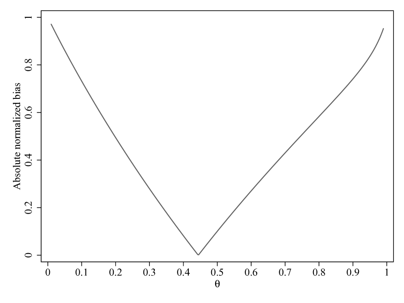
Figure 1: Estimated Bias of $\hat{\beta}_{\mathrm{RIV}}$

Notes: The data are Card (1995)’s subsample of the National Longitudinal Survey of Young Men (NLSYM). The sample and the covariate specification are as in Table 2. The dependent variable is log wages in 1976. The treatment variable is college attendance, which is defined as strictly more than twelve years of schooling. College attendance is instrumented by the “reordered” instrument that takes the value 1 for this value of the original instrument that is estimated to encourage treatment conditional on covariates and the value 0 otherwise. The original instrument is an indicator for whether an individual grew up in the vicinity of a four-year college. The vertical axis represents sample analogues of $\frac{\beta_{\mathrm{IV}}-\tau_{\mathrm{LATE}}}{\tau_{\mathrm{LATT}}-\tau_{\mathrm{LATU}}}$, where $\beta_{\mathrm{IV}}$ is replaced with the “reordered” IV estimate, $\hat{\beta}_{\mathrm{RIV}}$, and $\tau_{\mathrm{LATE}}$, $\tau_{\mathrm{LATT}}$, and $\tau_{\mathrm{LATU}}$ are estimated nonparametrically. The horizontal axis represents the implied values of $\theta$, that is, the proportion of individuals that are encouraged to get treated. All estimates are obtained using a weighted estimation procedure, with weights of 1 for individuals that are encouraged to get treated and weights of $w$ for individuals that are not encouraged to get treated. The variation in $w$ results in the variation that is represented in this figure.

But what if some of the assumptions above are indeed violated? To see this, I estimate $\tau_{\mathrm{LATE}}$, $\tau_{\mathrm{LATT}}$, and $\tau_{\mathrm{LATU}}$ nonparametrically, and use these estimates to construct sample analogues of $\frac{\beta_{\mathrm{IV}}-\tau_{\mathrm{LATE}}}{\tau_{\mathrm{LATT}}-\tau_{\mathrm{LATU}}}$, where none of the additional assumptions in Section 4 needs to hold. I also repeat this procedure multiple times, reestimating the (reordered) IV estimand, too, and using weights of 1 for individuals that are encouraged to get treated and weights of $w$ for individuals that are not encouraged to get treated. As I vary the value of $w$, I am able to manipulate the implied value of $\theta$ without affecting other relevant features of the data-generating process.

Figure 1 shows that the rule of thumb based on Corollary 4.3 is strikingly accurate in this application. The estimated bias is clearly dependent on the proportion of individuals that are encouraged to get treated. Indeed, the bias is approximately zero when the implied value of $\theta$ is about 0.445, which is similar to the rule-of-thumb value of 0.5. The bias is also increasing in the distance between the implied value of $\theta$ and 0.445, approaching 100% of the difference between $\hat{\tau}_{\mathrm{LATT}}$ and $\hat{\tau}_{\mathrm{LATU}}$ when almost no or almost all individuals are encouraged to get treated.

The bottom line is that the IV estimand does not need to be similar to the unconditional LATE parameter even in the arguably optimistic scenario when Assumptions IV, SM, and PS hold; also, the dissimilarity between these parameters turns out to depend on $\theta$ and a simple measure of treatment effect heterogeneity.

6 Conclusion

In this paper I study the interpretation of linear IV and 2SLS estimands when both the endogenous treatment and the instrument are binary, and when additional covariates are required for identification. I follow the LATE framework of Imbens and Angrist (1994) and Angrist et al. (1996), and conclude that the common practice of interpreting linear IV and 2SLS estimands as a convex combination of conditional LATEs, or even as “the” (unconditional) LATE, is substantially more problematic than previously thought. In an important paper, Kolesár (2013) concludes that the weights on all conditional LATEs are guaranteed to be positive, subject to some additional assumptions about the first stage, even when there are compliers but no defiers at some covariate values and defiers but no compliers elsewhere. In this paper I demonstrate that, under this weaker version of monotonicity, Kolesár (2013)’s assumptions about the first stage are not satisfied in the usual application of IV that limits the effects of the instrument in the reduced-form and first-stage regressions to be homogeneous. Consequently, some of the IV weights will be negative and the IV estimand may no longer be interpretable as a causal effect; this parameter may turn out to be negative (positive) even if treatment effects are universally positive (negative).

While there are several lessons to be learned from my theoretical results, the simplest takeaway from this paper is that in many applications of IV methods two robustness checks are in order. First, reporting an estimate from the overidentified specification of Angrist and Imbens (1995) or the “reordered IV” procedure of this paper would provide a robustness check against the presence of negative weights. (One must use caution because these two procedures are also less robust to problems with weak instruments.) Second, to check whether the IV and 2SLS estimands are not too different from the unconditional LATE parameter, it would also be useful to report a direct estimate of this latter object, perhaps based on the approach of Tan (2006), Frölich (2007), Hong and Nekipelov (2010), Donald et al. (2014), Sant’Anna et al. (2021), or Słoczyński et al. (2022). This second robustness check is important because the lack of negative weights is not sufficient for an estimand to correspond to an interesting target parameter (cf. Callaway et al., 2021; Callaway and Sant’Anna, 2021). It does indeed seem that many empirical studies actually intend to focus on the unconditional LATE parameter. I show that it is more appropriate to claim similarity between the IV estimand and “the” (unconditional) LATE when the groups with different values of the instrument are roughly equal sized. Of course, the difference between these two objects can always be examined empirically, which is precisely what I recommend as the second robustness check.

Appendix A Proofs

Proof of Theorem 3.3.

Let $R$ and $T$ be generic notation for two random variables, where $T$ is binary and $R$ is arbitrarily discrete or continuous. The following lemma, due to Angrist (1998), will be useful for what follows.

Lemma A.1 (Angrist, 1998).

Suppose that $\mathrm{E}\left[T\mid X\right]$ is linear in $X$. Then, $\xi$, the coefficient on $T$ in the linear projection of $R$ on $T$ and $X$ can be written as

$$\xi=\frac{\mathrm{E}\left[\mathrm{Var}\left[T\mid X\right]\cdot\xi(X)\right]}{\mathrm{E}\left[\mathrm{Var}\left[T\mid X\right]\right]},$$

where $\xi(X)=\mathrm{E}\left[R\mid T=1,X\right]-\mathrm{E}\left[R\mid T=0,X\right]$.

Recall that $\beta_{\mathrm{IV}}$ is equal to the ratio of the reduced-form and first-stage coefficients on $Z$. It follows that we can apply Lemma A.1 separately to these two coefficients, and thereby obtain the following expression for the estimand of interest:

$$\beta_{\mathrm{IV}}=\frac{\frac{\mathrm{E}\left[\mathrm{Var}\left[Z\mid X\right]\cdot\phi(X)\right]}{\mathrm{E}\left[\mathrm{Var}\left[Z\mid X\right]\right]}}{\frac{\mathrm{E}\left[\mathrm{Var}\left[Z\mid X\right]\cdot\omega(X)\right]}{\mathrm{E}\left[\mathrm{Var}\left[Z\mid X\right]\right]}},$$ (25)

where

$$\phi(x)=\mathrm{E}\left[Y\mid Z=1,X=x\right]-\mathrm{E}\left[Y\mid Z=0,X=x\right]$$ (26)

is the conditional reduced-form slope coefficient and $\omega(x)$ is as defined in equation (5). Upon rearrangement, we obtain

$$\beta_{\mathrm{IV}} = \frac{\mathrm{E}\left[\mathrm{Var}\left[Z\mid X\right]\cdot\phi(X)\right]}{\mathrm{E}\left[\mathrm{Var}\left[Z\mid X\right]\cdot\omega(X)\right]}$$ (27)

$$= \frac{\mathrm{E}\left[\mathrm{Var}\left[Z\mid X\right]\cdot\omega(X)\cdot\beta(X)\right]}{\mathrm{E}\left[\mathrm{Var}\left[Z\mid X\right]\cdot\omega(X)\right]},$$

where the second equality uses the definition of $\beta(x)$ in equation (6). See also Walters (2018) for a similar argument. Finally, we know from Lemma 2.1 that $\beta(x)=\tau(x)$ and $\omega(x)=c(x)\cdot\pi(x)$ under Assumptions IV and WM. This completes the proof because $\beta_{\mathrm{IV}}$ can now be written as

$$\beta_{\mathrm{IV}}=\frac{\mathrm{E}\left[c(X)\cdot\pi(X)\cdot\mathrm{Var}\left[Z\mid X\right]\cdot\tau(X)\right]}{\mathrm{E}\left[c(X)\cdot\pi(X)\cdot\mathrm{Var}\left[Z\mid X\right]\right]}.$$ (28)

Proof of Theorem 3.5.

The assumption that the conditional mean of the instrument is linear in $X$ underlies the proof of Theorem 3.3, including equation (27). Under this assumption, we can use equation (27) to write

$$\beta_{\mathrm{RIV}}=\frac{\mathrm{E}\left[\mathrm{Var}\left[Z_{\mathrm{R}}\mid X\right]\cdot\omega_{\mathrm{R}}(X)\cdot\beta_{\mathrm{R}}(X)\right]}{\mathrm{E}\left[\mathrm{Var}\left[Z_{\mathrm{R}}\mid X\right]\cdot\omega_{\mathrm{R}}(X)\right]},$$ (29)

where

$$\omega_{\mathrm{R}}(x)=\mathrm{E}\left[D\mid Z_{\mathrm{R}}=1,X=x\right]-\mathrm{E}\left[D\mid Z_{\mathrm{R}}=0,X=x\right]$$ (30)

and

$$\beta_{\mathrm{R}}(x)=\frac{\phi_{\mathrm{R}}(x)}{\omega_{\mathrm{R}}(x)},$$ (31)

where

$$\phi_{\mathrm{R}}(x)=\mathrm{E}\left[Y\mid Z_{\mathrm{R}}=1,X=x\right]-\mathrm{E}\left[Y\mid Z_{\mathrm{R}}=0,X=x\right].$$ (32)

Then, it is important to see that $\omega_{\mathrm{R}}(x)=\omega(x)$ and $\phi_{\mathrm{R}}(x)=\phi(x)$ if $\omega(x)>0$, $\omega_{\mathrm{R}}(x)=-\omega(x)$ and $\phi_{\mathrm{R}}(x)=-\phi(x)$ if $\omega(x)<0$, and consequently $\beta_{\mathrm{R}}(x)=\beta(x)$ regardless of the sign of $\omega(x)$. We can also write $\omega_{\mathrm{R}}(x)=c(x)\cdot\omega(x)$, $\phi_{\mathrm{R}}(x)=c(x)\cdot\phi(x)$, and $\mathrm{Var}\left[Z_{\mathrm{R}}\mid X=x\right]=\mathrm{Var}\left[Z\mid X=x\right]$ regardless of the sign of $\omega(x)$. It follows that

$$\beta_{\mathrm{RIV}}=\frac{\mathrm{E}\left[\mathrm{Var}\left[Z\mid X\right]\cdot c(X)\cdot\omega(X)\cdot\beta(X)\right]}{\mathrm{E}\left[\mathrm{Var}\left[Z\mid X\right]\cdot c(X)\cdot\omega(X)\right]}.$$ (33)

To complete this proof, note that, under Assumptions IV and WM, we know from Lemma 2.1 that $\beta(x)=\tau(x)$ and $\omega(x)=c(x)\cdot\pi(x)$. Also, $\left[c(x)\right]^{2}=1$ because $c(x)\in\{-1,1\}$. Thus, it follows that

$$\beta_{\mathrm{RIV}} = \frac{\mathrm{E}\left[\mathrm{Var}\left[Z\mid X\right]\cdot\left[c(X)\right]^{2}\cdot\pi(X)\cdot\tau(X)\right]}{\mathrm{E}\left[\mathrm{Var}\left[Z\mid X\right]\cdot\left[c(X)\right]^{2}\cdot\pi(X)\right]}$$ (34)

$$= \frac{\mathrm{E}\left[\mathrm{Var}\left[Z\mid X\right]\cdot\pi(X)\cdot\tau(X)\right]}{\mathrm{E}\left[\mathrm{Var}\left[Z\mid X\right]\cdot\pi(X)\right]}.$$

This completes the proof.

Proof of Theorem 4.1.

Let us use the same notation as in the proof of Theorem 3.3. If $\mathrm{L}\left[\cdot\mid\cdot\right]$ denotes the linear projection, let $p(X)$ denote the best linear approximation to the “propensity score” for $T$; that is,

$$p(X)=\mathrm{L}\left[T\mid X\right]=X\rho,$$ (35)

with $X$ being completely general and not necessarily consisting only of group indicators. We also need two linear projections of $R$ on $1$ and $p(X)$, separately for $T=1$ and $T=0$; that is,

$$\mathrm{L}\left[R\mid 1,p(X),T=t\right]=\iota_{t}+\zeta_{t}\cdot p(X).$$ (36)

The following lemma, due to Słoczyński (2022), will be useful for what follows.

Lemma A.2 (Słoczyński, 2022).

The coefficient on $T$ in the linear projection of $R$ on $T$ and $X$, denoted by $\xi$, can be written as

$$\xi = w_{1}\cdot\big{(}\left(\iota_{1}-\iota_{0}\right)+\left(\zeta_{1}-\zeta_{0}\right)\cdot\mathrm{E}\left[p(X)\mid T=1\right]\big{)}$$

$$+ w_{0}\cdot\big{(}\left(\iota_{1}-\iota_{0}\right)+\left(\zeta_{1}-\zeta_{0}\right)\cdot\mathrm{E}\left[p(X)\mid T=0\right]\big{)},$$

where $w_{1}=\frac{\mathrm{P}\left[T=0\right]\cdot\mathrm{Var}\left[p(X)\mid T=0\right]}{\mathrm{P}\left[T=1\right]\cdot\mathrm{Var}\left[p(X)\mid T=1\right]\;+\;\mathrm{P}\left[T=0\right]\cdot\mathrm{Var}\left[p(X)\mid T=0\right]}$ and $w_{0}=\frac{\mathrm{P}\left[T=1\right]\cdot\mathrm{Var}\left[p(X)\mid T=1\right]}{\mathrm{P}\left[T=1\right]\cdot\mathrm{Var}\left[p(X)\mid T=1\right]\;+\;\mathrm{P}\left[T=0\right]\cdot\mathrm{Var}\left[p(X)\mid T=0\right]}$.

Again, we can use the fact that $\beta_{\mathrm{IV}}$ is equal to the ratio of the reduced-form and first-stage coefficients on $Z$, and apply Lemma A.2 separately to these coefficients. Thus, $Y$ will play the role of $R$ in the reduced-form regression, $D$ will play the role of $R$ in the first-stage regression, and $Z$ will play the role of $T$ in both regressions. Additionally, under Assumption PS, equation (35) corresponds to the true instrument propensity score and, under Assumption LN, equation (36) represents the true reduced-form and first-stage regressions. It follows from Lemma A.2 that under these assumptions the reduced-form and first-stage coefficients on $Z$ are equal to a convex combination of the average causal effects of $Z$ on $Y$ and $D$ in the subpopulations with $Z=1$ and $Z=0$, with weights equal to $w_{1}^{\ast}=\frac{\left(1-\theta\right)\cdot\mathrm{Var}\left[e(X)\mid Z=0\right]}{\theta\cdot\mathrm{Var}\left[e(X)\mid Z=1\right]\;+\;\left(1-\theta\right)\cdot\mathrm{Var}\left[e(X)\mid Z=0\right]}$ and $w_{0}^{\ast}=\frac{\theta\cdot\mathrm{Var}\left[e(X)\mid Z=1\right]}{\theta\cdot\mathrm{Var}\left[e(X)\mid Z=1\right]\;+\;\left(1-\theta\right)\cdot\mathrm{Var}\left[e(X)\mid Z=0\right]}$, respectively. Indeed,

$$\beta_{\mathrm{IV}} = \frac{w_{1}^{\ast}\cdot\mathrm{E}\left[Y(D(1))-Y(D(0))\mid Z=1\right]\;+\;w_{0}^{\ast}\cdot\mathrm{E}\left[Y(D(1))-Y(D(0))\mid Z=0\right]}{w_{1}^{\ast}\cdot\pi_{1}\;+\;w_{0}^{\ast}\cdot\pi_{0}}$$ (37)

$$= \frac{w_{1}^{\ast}\cdot\pi_{1}\cdot\tau_{\mathrm{LATT}}\;+\;w_{0}^{\ast}\cdot\pi_{0}\cdot\tau_{\mathrm{LATU}}}{w_{1}^{\ast}\cdot\pi_{1}\;+\;w_{0}^{\ast}\cdot\pi_{0}}$$

$$= \frac{\left(1-\theta\right)\cdot\mathrm{Var}\left[e(X)\mid Z=0\right]\cdot\pi_{1}\cdot\tau_{\mathrm{LATT}}\;+\;\theta\cdot\mathrm{Var}\left[e(X)\mid Z=1\right]\cdot\pi_{0}\cdot\tau_{\mathrm{LATU}}}{\left(1-\theta\right)\cdot\mathrm{Var}\left[e(X)\mid Z=0\right]\cdot\pi_{1}\;+\;\theta\cdot\mathrm{Var}\left[e(X)\mid Z=1\right]\cdot\pi_{0}}$$

$$= w_{\mathrm{LATT}}\cdot\tau_{\mathrm{LATT}}\;+\;w_{\mathrm{LATU}}\cdot\tau_{\mathrm{LATU}},$$

where the second equality uses the fact that $\tau_{\mathrm{LATT}}=\frac{\mathrm{E}\left[Y(D(1))-Y(D(0))\mid Z=1\right]}{\mathrm{E}\left[D(1)-D(0)\mid Z=1\right]}$ (see, e.g., Frölich and Lechner, 2010) and likewise $\tau_{\mathrm{LATU}}=\frac{\mathrm{E}\left[Y(D(1))-Y(D(0))\mid Z=0\right]}{\mathrm{E}\left[D(1)-D(0)\mid Z=0\right]}$; also, $\pi_{z}=\mathrm{E}\left[D(1)-D(0)\mid Z=z\right]$ under Assumption SM. The remaining equalities follow from simple algebra. This completes the proof.

Proof of Corollary 4.3.

Under Assumption HS, it follows from Theorem 4.1 that

$$\beta_{\mathrm{IV}}\;=\;\frac{\left(1-\theta\right)\cdot\pi_{1}}{\theta\cdot\pi_{0}\;+\;\left(1-\theta\right)\cdot\pi_{1}}\cdot\tau_{\mathrm{LATT}}\;+\;\frac{\theta\cdot\pi_{0}}{\theta\cdot\pi_{0}\;+\;\left(1-\theta\right)\cdot\pi_{1}}\cdot\tau_{\mathrm{LATU}}.$$ (38)

We also know from equation (20) that

$$\tau_{\mathrm{LATE}}\;=\;\frac{\theta\cdot\pi_{1}}{\theta\cdot\pi_{1}\;+\;\left(1-\theta\right)\cdot\pi_{0}}\cdot\tau_{\mathrm{LATT}}\;+\;\frac{\left(1-\theta\right)\cdot\pi_{0}}{\theta\cdot\pi_{1}\;+\;\left(1-\theta\right)\cdot\pi_{0}}\cdot\tau_{\mathrm{LATU}}.$$ (39)

The proof consists of three steps. First, we need to show that $\tau_{\mathrm{LATT}}=\tau_{\mathrm{LATU}}$ implies that $\beta_{\mathrm{IV}}=\tau_{\mathrm{LATE}}$. This follows immediately from equations (38) and (39) as both $\beta_{\mathrm{IV}}$ and $\tau_{\mathrm{LATE}}$ are convex combinations of $\tau_{\mathrm{LATT}}$ and $\tau_{\mathrm{LATU}}$. In fact, this implication does not even rely on Assumption HS.

Second, we need to show that $\theta=0.5$ implies that $\beta_{\mathrm{IV}}=\tau_{\mathrm{LATE}}$. Indeed, if $\theta=0.5$, then it follows from equation (38) that

$$\beta_{\mathrm{IV}}\;=\;\frac{\pi_{1}}{\pi_{0}+\pi_{1}}\cdot\tau_{\mathrm{LATT}}\;+\;\frac{\pi_{0}}{\pi_{0}+\pi_{1}}\cdot\tau_{\mathrm{LATU}}.$$ (40)

Similarly, it follows from equation (39) that

$$\tau_{\mathrm{LATE}}\;=\;\frac{\pi_{1}}{\pi_{0}+\pi_{1}}\cdot\tau_{\mathrm{LATT}}\;+\;\frac{\pi_{0}}{\pi_{0}+\pi_{1}}\cdot\tau_{\mathrm{LATU}},$$ (41)

and hence $\beta_{\mathrm{IV}}=\tau_{\mathrm{LATE}}$.

Finally, we need to show that $\beta_{\mathrm{IV}}=\tau_{\mathrm{LATE}}$ implies that either $\tau_{\mathrm{LATT}}=\tau_{\mathrm{LATU}}$ or $\theta=0.5$. We begin by equating the right-hand sides of equations (38) and (39). Upon rearrangement, we get

$$\frac{\theta\cdot\chi_{0}\;+\;\left(1-\theta\right)\cdot\chi_{1}}{\theta\cdot\pi_{0}\;+\;\left(1-\theta\right)\cdot\pi_{1}}\;=\;\frac{\theta\cdot\chi_{1}\;+\;\left(1-\theta\right)\cdot\chi_{0}}{\theta\cdot\pi_{1}\;+\;\left(1-\theta\right)\cdot\pi_{0}},$$ (42)

where

$$\chi_{z}=\mathrm{E}\left[Y(D(1))-Y(D(0))\mid Z=z\right].$$ (43)

Upon further rearrangement of equation (42), we obtain

$$\theta^{2}\cdot\chi_{0}\cdot\pi_{1}\;+\;\left(1-\theta\right)^{2}\cdot\chi_{1}\cdot\pi_{0}\;=\;\theta^{2}\cdot\chi_{1}\cdot\pi_{0}\;+\;\left(1-\theta\right)^{2}\cdot\chi_{0}\cdot\pi_{1},$$ (44)

which also implies that

$$\left(\chi_{0}\cdot\pi_{1}-\chi_{1}\cdot\pi_{0}\right)\cdot\left(2\theta-1\right)\;=\;0.$$ (45)

For equation (45) to hold, we need either $\theta=0.5$ or $\frac{\chi_{1}}{\pi_{1}}=\frac{\chi_{0}}{\pi_{0}}$, where the latter condition is equivalent to $\tau_{\mathrm{LATT}}=\tau_{\mathrm{LATU}}$. This completes the proof.

References

- Abadie (2003) Abadie, Alberto (2003): “Semiparametric Instrumental Variable Estimation of Treatment Response Models,” Journal of Econometrics, 113, 231–263.
- Abadie et al. (2019) Abadie, Alberto, Jiaying Gu, and Shu Shen (2019): “Instrumental Variable Estimation with First-Stage Heterogeneity.” Unpublished.
- Aizer and Doyle (2015) Aizer, Anna and Joseph J. Doyle (2015): “Juvenile Incarceration, Human Capital, and Future Crime: Evidence from Randomly Assigned Judges,” Quarterly Journal of Economics, 130, 759–804.
- Andresen and Huber (2021) Andresen, Martin E. and Martin Huber (2021): “Instrument-Based Estimation with Binarised Treatments: Issues and Tests for the Exclusion Restriction,” Econometrics Journal, 24, 536–558.
- Angrist (1990) Angrist, Joshua D. (1990): “Lifetime Earnings and the Vietnam Era Draft Lottery: Evidence from Social Security Administrative Records,” American Economic Review, 80, 313–336.
- Angrist (1998) ——— (1998): “Estimating the Labor Market Impact of Voluntary Military Service Using Social Security Data on Military Applicants,” Econometrica, 66, 249–288.
- Angrist and Imbens (1995) Angrist, Joshua D. and Guido W. Imbens (1995): “Two-Stage Least Squares Estimation of Average Causal Effects in Models with Variable Treatment Intensity,” Journal of the American Statistical Association, 90, 431–442.
- Angrist et al. (1996) Angrist, Joshua D., Guido W. Imbens, and Donald B. Rubin (1996): “Identification of Causal Effects Using Instrumental Variables,” Journal of the American Statistical Association, 91, 444–455.
- Angrist and Krueger (1991) Angrist, Joshua D. and Alan B. Krueger (1991): “Does Compulsory School Attendance Affect Schooling and Earnings?” Quarterly Journal of Economics, 106, 979–1014.
- Angrist and Pischke (2009) Angrist, Joshua D. and Jörn-Steffen Pischke (2009): Mostly Harmless Econometrics: An Empiricist’s Companion, Princeton–Oxford: Princeton University Press.
- Autor et al. (2019) Autor, David, Andreas Kostøl, Magne Mogstad, and Bradley Setzler (2019): “Disability Benefits, Consumption Insurance, and Household Labor Supply,” American Economic Review, 109, 2613–2654.
- Blandhol et al. (2022) Blandhol, Christine, John Bonney, Magne Mogstad, and Alexander Torgovitsky (2022): “When Is TSLS Actually LATE?” NBER Working Paper no. 29709.
- Bond et al. (2007) Bond, Simon J., Ian R. White, and A. Sarah Walker (2007): “Instrumental Variables and Interactions in the Causal Analysis of a Complex Clinical Trial,” Statistics in Medicine, 26, 1473–1496.
- Bondy et al. (2020) Bondy, Malvina, Sefi Roth, and Lutz Sager (2020): “Crime Is in the Air: The Contemporaneous Relationship between Air Pollution and Crime,” Journal of the Association of Environmental and Resource Economists, 7, 555–585.
- Bound et al. (1995) Bound, John, David A. Jaeger, and Regina M. Baker (1995): “Problems with Instrumental Variables Estimation When the Correlation between the Instruments and the Endogenous Explanatory Variable Is Weak,” Journal of the American Statistical Association, 90, 443–450.
- Caetano and Escanciano (2021) Caetano, Carolina and Juan Carlos Escanciano (2021): “Identifying Multiple Marginal Effects with a Single Instrument,” Econometric Theory, 37, 464–494.
- Callaway et al. (2021) Callaway, Brantly, Andrew Goodman-Bacon, and Pedro H. C. Sant’Anna (2021): “Difference-in-Differences with a Continuous Treatment,” arXiv:2107.02637v2.
- Callaway and Sant’Anna (2021) Callaway, Brantly and Pedro H. C. Sant’Anna (2021): “Difference-in-Differences with Multiple Time Periods,” Journal of Econometrics, 225, 200–230.
- Cameron and Taber (2004) Cameron, Stephen V. and Christopher Taber (2004): “Estimation of Educational Borrowing Constraints Using Returns to Schooling,” Journal of Political Economy, 112, 132–182.
- Card (1995) Card, David (1995): “Using Geographic Variation in College Proximity to Estimate the Return to Schooling,” in Aspects of Labour Market Behaviour: Essays in Honour of John Vanderkamp, ed. by L. N. Christofides, E. K. Grant, and R. Swidinsky, Toronto: University of Toronto Press.
- Carneiro et al. (2011) Carneiro, Pedro, James J. Heckman, and Edward J. Vytlacil (2011): “Estimating Marginal Returns to Education,” American Economic Review, 101, 2754–2781.
- Dahl et al. (2019) Dahl, Christian M., Martin Huber, and Giovanni Mellace (2019): “It’s Never Too LATE: A New Look at Local Average Treatment Effects with or without Defiers.” Unpublished.
- de Chaisemartin (2017) de Chaisemartin, Clément (2017): “Tolerating Defiance? Local Average Treatment Effects without Monotonicity,” Quantitative Economics, 8, 367–396.
- Deryugina et al. (2019) Deryugina, Tatyana, Garth Heutel, Nolan H. Miller, David Molitor, and Julian Reif (2019): “The Mortality and Medical Costs of Air Pollution: Evidence from Changes in Wind Direction,” American Economic Review, 109, 4178–4219.
- Dinkelman (2011) Dinkelman, Taryn (2011): “The Effects of Rural Electrification on Employment: New Evidence from South Africa,” American Economic Review, 101, 3078–3108.
- Dobbie et al. (2018) Dobbie, Will, Jacob Goldin, and Crystal S. Yang (2018): “The Effects of Pretrial Detention on Conviction, Future Crime, and Employment: Evidence from Randomly Assigned Judges,” American Economic Review, 108, 201–240.
- Donald et al. (2014) Donald, Stephen G., Yu-Chin Hsu, and Robert P. Lieli (2014): “Testing the Unconfoundedness Assumption via Inverse Probability Weighted Estimators of (L)ATT,” Journal of Business & Economic Statistics, 32, 395–415.
- Eisenhauer et al. (2015) Eisenhauer, Philipp, James J. Heckman, and Edward Vytlacil (2015): “The Generalized Roy Model and the Cost-Benefit Analysis of Social Programs,” Journal of Political Economy, 123, 413–443.
- Evdokimov and Kolesár (2019) Evdokimov, Kirill S. and Michal Kolesár (2019): “Inference in Instrumental Variables Analysis with Heterogeneous Treatment Effects.” Unpublished.
- Finkelstein et al. (2012) Finkelstein, Amy, Sarah Taubman, Bill Wright, Mira Bernstein, Jonathan Gruber, Joseph P. Newhouse, Heidi Allen, Katherine Baicker, and Oregon Health Study Group (2012): “The Oregon Health Insurance Experiment: Evidence from the First Year,” Quarterly Journal of Economics, 127, 1057–1106.
- Frandsen et al. (2019) Frandsen, Brigham R., Lars J. Lefgren, and Emily C. Leslie (2019): “Judging Judge Fixed Effects,” NBER Working Paper no. 25528.
- Frölich (2007) Frölich, Markus (2007): “Nonparametric IV Estimation of Local Average Treatment Effects with Covariates,” Journal of Econometrics, 139, 35–75.
- Frölich and Lechner (2010) Frölich, Markus and Michael Lechner (2010): “Exploiting Regional Treatment Intensity for the Evaluation of Labor Market Policies,” Journal of the American Statistical Association, 105, 1014–1029.
- Frölich and Sperlich (2019) Frölich, Markus and Stefan Sperlich (2019): Impact Evaluation: Treatment Effects and Causal Analysis, Cambridge: Cambridge University Press.
- Heckman et al. (2006) Heckman, James J., Sergio Urzua, and Edward Vytlacil (2006): “Understanding Instrumental Variables in Models with Essential Heterogeneity,” Review of Economics and Statistics, 88, 389–432.
- Heckman and Vytlacil (2005) Heckman, James J. and Edward Vytlacil (2005): “Structural Equations, Treatment Effects, and Econometric Policy Evaluation,” Econometrica, 73, 669–738.
- Hoekstra (2009) Hoekstra, Mark (2009): “The Effect of Attending the Flagship State University on Earnings: A Discontinuity-Based Approach,” Review of Economics and Statistics, 91, 717–724.
- Hong and Nekipelov (2010) Hong, Han and Denis Nekipelov (2010): “Semiparametric Efficiency in Nonlinear LATE Models,” Quantitative Economics, 1, 279–304.
- Humphreys (2009) Humphreys, Macartan (2009): “Bounds on Least Squares Estimates of Causal Effects in the Presence of Heterogeneous Assignment Probabilities.” Unpublished.
- Huntington-Klein (2020) Huntington-Klein, Nick (2020): “Instruments with Heterogeneous Effects: Bias, Monotonicity, and Localness,” Journal of Causal Inference, 8, 182–208.
- Imbens and Angrist (1994) Imbens, Guido W. and Joshua D. Angrist (1994): “Identification and Estimation of Local Average Treatment Effects,” Econometrica, 62, 467–475.
- Ishimaru (2021) Ishimaru, Shoya (2021): “Empirical Decomposition of the IV–OLS Gap with Heterogeneous and Nonlinear Effects,” Review of Economics and Statistics, forthcoming.
- Kane and Rouse (1993) Kane, Thomas J. and Cecilia Elena Rouse (1993): “Labor Market Returns to Two- and Four-Year Colleges: Is a Credit a Credit and Do Degrees Matter?” NBER Working Paper no. 4268.
- Kitagawa (2015) Kitagawa, Toru (2015): “A Test for Instrument Validity,” Econometrica, 83, 2043–2063.
- Kline et al. (2022) Kline, Patrick, Evan K. Rose, and Christopher R. Walters (2022): “Systemic Discrimination among Large U.S. Employers,” Quarterly Journal of Economics, forthcoming.
- Kling (2001) Kling, Jeffrey R. (2001): “Interpreting Instrumental Variables Estimates of the Returns to Schooling,” Journal of Business & Economic Statistics, 19, 358–364.
- Kolesár (2013) Kolesár, Michal (2013): “Estimation in an Instrumental Variables Model with Treatment Effect Heterogeneity.” Unpublished.