Greedy Motzkin-Kaczmarz methods for solving linear systems

Abstract

[Summary]The famous greedy randomized Kaczmarz (GRK) method uses the greedy selection rule on maximum distance to determine a subset of the indices of working rows. In this paper, with the greedy selection rule on maximum residual, we propose the greedy randomized Motzkin-Kaczmarz (GRMK) method for linear systems. The block version of the new method is also presented. We analyze the convergence of the two methods and provide the corresponding convergence factors. Extensive numerical experiments show that the GRMK method has almost the same performance as the GRK method for dense matrices and the former performs better in computing time for some sparse matrices, and the block versions of the GRMK and GRK methods always have almost the same performance.

1 Introduction

We consider the following consistent linear systems

$$Ax=b,$$ (1)

where $A\in R^{m\times n}$, $b\in R^{m}$, and $x$ is the $n$-dimensional unknown vector. As we know, the Kaczmarz method ¹ is a popular so-called row-action method for solving the systems (1). Its update formula is

$$x_{k+1}=x_{k}+\frac{b^{(i)}-A^{(i)}x_{k}}{\|A^{\left(i\right)}\|_{2}^{2}}(A^{(i)})^{T},$$ (2)

where $A^{(i)}$ denotes the $i$-th row of $A$, $b^{(i)}$ denotes the $i$-th entry of $b$, and $A^{T}$ denotes the transpose of $A$. In 2009, Strohmer and Vershynin ² show that the Kaczmarz method converges with expected exponential rate if the row of $A$ in iteration is chosen randomly with probability proportional to the square of the Euclidean norm of the row. Subsequently, many randomized Kaczmarz type methods were proposed for different possible systems settings; see for example ^{3, 4, 5, 6} and references therein. These randomized methods have two obvious disadvantages. The first one is that the probability criterion will be equivalent to the uniform sampling if the Euclidean norms of all the rows of the matrix $A$ are the same. The case can happen by scaling the matrix $A$ with a suitable diagonal matrix. The second one is that it is possible to sample the same row twice in iteration. In this case, no progress is made in such an update. To tackle these problems, in 2018, Bai and Wu ⁷ constructed a greedy randomized Kaczmarz (GRK) method by introducing a more efficient probability criterion for selecting the working rows from the matrix $A$. The GRK method outperforms the ordinary randomized Kaczmarz methods in terms of the number of iterations and computing time, and the scheme in this method is very powerful in achieving efficient methods for solving linear problems ^{8, 9, 10}, least squares problem ^{11, 12} and ridge regression problem¹³.

The greedy selection rule used in the GRK method is from the well known maximum distance rule because the index subset in the method is built on the combination of the maximum and average distances. As we know, there are two main famous greedy selection rules: the maximum distance rule and the maximum residual rule. Specifically, let $x_{\star}=A^{{\dagger}}b$ be the least-Euclidean-norm solution of the systems (1). Then a sequence of vectors $x_{0}$, $x_{1}$, …produced by the iteration (2) is said to converge in square to the solution $x_{\star}$ if and only if $\|x_{k}-x_{\star}\|^{2}_{2}\rightarrow 0$ as $k\rightarrow\infty$. Since the projections in iteration are orthogonal, we can check that (see also the proof of Theorem 3.3 below)

$$\|x_{k+1}-x_{\star}\|^{2}_{2}=\|x_{k}-x_{\star}\|^{2}_{2}-\|x_{k+1}-x_{k}\|^{2}_{2}.$$

Hence, the optimal projection is the one that maximizes the distances $\|x_{k+1}-x_{k}\|^{2}_{2}$. Note that the update formula (2) implies

$$\|x_{k+1}-x_{k}\|^{2}_{2}=\left\|\frac{b^{(i)}-A^{(i)}x_{k}}{\|A^{(i)}\|_{2}^{2}}(A^{(i)})^{T}\right\|^{2}_{2},$$

which shows that in iteration we should select the $t_{k}$-th index according to

$$t_{k}={\rm arg}\max\limits_{i}\left\|\frac{b^{(i)}-A^{(i)}x_{k}}{\|A^{(i)}\|_{2}^{2}}(A^{(i)})^{T}\right\|^{2}_{2}={\rm arg}\max\limits_{i}\frac{(b^{(i)}-A^{(i)}x_{k})^{2}}{\|A^{(i)}\|^{2}_{2}}.$$

This greedy selection rule is the maximum distance rule ^{14, 15, 16}. The maximum residual rule ^{17, 16} selects the $t_{k}$-th index according to

$$t_{k}={\rm arg}\max\limits_{i}(b^{(i)}-A^{(i)}x_{k})^{2}.$$

That is, it grasps the index corresponding to the largest magnitude entry of the residual vector $r_{k}=b-Ax_{k}$, and hence the largest magnitude entry of the residual vector $r_{k}$ can be preferentially annihilated as far as possible and make the $t_{k}$-th equation be ‘furthest’ from being satisfied. The maximum residual rule is also known as the Motzkin method ^{18, 19}, which can also make sure that the same index will not be chosen twice in iteration and hence has better convergence rate compared with the ordinary randomized Kaczmarz methods. Consequently, many analyses and applications about Motzkin type methods were published in recent years; see for example ^{20, 21, 22, 23, 24, 25, 26} and references therein.

However, to the best of our knowledge, there are few results in the literature that explore the use of greedy randomized Motzkin scheme, i.e., the maximum residual rule, for Kaczmarz type algorithms for solving linear systems. To fill the research gap, in this work, paralleling to the GRK method, we develop the greedy randomized Kaczmarz method induced from the Motzkin method, i.e., the greedy randomized Motzkin-Kaczmarz (GRMK) method, for solving the systems (1). Moreover, to further accelerate the GRMK method, we also present the block version of the new method using the index subset generated in the GRMK method and refer to it as the greedy Motzkin block Kaczmarz (GMBK) method. Recently, many works on block Kaczmarz methods were reported because, compared with the original methods, the block methods allows for significant computational speedup and accelerated convergence to the solution; see for example ^{27, 28, 29, 30}. The block update formula can be written as

$$x_{k+1}=x_{k}+A^{\dagger}_{\tau}(b_{\tau}-A_{\tau}x_{k}),$$ (3)

where $\tau\subset\{1,\ldots,m\}$, $A_{\tau}$ and $b_{\tau}$ are the submatrix and subvector of $A$ and $b$, respectively, with rows indexed by $\tau$, and $A^{\dagger}_{\tau}$ is the Moore-Penrose pseudoinverse of $A_{\tau}$. To avoid computing the pseudoinverse, a variant of the above block Kaczmarz method is to project the current estimate onto each individual row that forms the submatrix $A_{\tau}$, and average the obtained projections to form the next iterate:

$$x_{k+1}=x_{k}-\sum_{i\in{\tau}}w_{i}\frac{A^{(i)}x_{k}-b^{(i)}}{\left\|A^{(i)}\right\|^{2}_{2}}(A^{(i)})^{T},$$ (4)

where $w_{i}$ represents the weight corresponding to the $i$-th row. This update is very suitable for distributed computing; see ^{31, 32, 33} for detailed discussions on this topic.

The rest of this paper is organized as follows. In Section 2, some notation and preliminaries are given. The GRMK method and its block version are discussed in Section 3 and Section 4, respectively. Finally, we present the numerical results in Section 5.

2 Notation and preliminaries

Throughout the paper, for a matrix $A$, ${\rm R(A)}$ denotes its column space, and for a set $\mathcal{I}$, $|\mathcal{I}|$ denotes the number of elements of the set. In addition, the smallest positive eigenvalues of $A^{T}A$ is denoted by $\lambda_{\min}(A^{T}A)$.

To analyze the convergence of our new methods, the following fact will be used extensively.

Lemma 2.1.

⁷ Let $A\in R^{m\times n}$ and for any vector $x\in{\rm R(A^{T})}$, it holds that

$$\|Ax\|^{2}_{2}\geq\lambda_{\min}\left(A^{T}A\right)\|x\|^{2}_{2}.$$

For comparison later in this paper, we list the GRK method proposed in ⁷ in Algorithm 1.

Algorithm 1.

The GRK method for the systems (1).

1. INPUT:  $A\in R^{m\times n}$, $b\in R^{m}$, $\ell$ , initial estimate $x_{0}$

2. OUTPUT:  $x_{\ell}$

3. For $k=0,1,2,\ldots,\ell-1$ do

4. Compute

   $$\epsilon_{k}=\frac{1}{2}\left(\max_{1\leq i_{k}\leq m}\left\{\frac{|r^{\left(i_{k}\right)}_{k}|^{2}}{\left\|A^{\left(i_{k}\right)}\right\|_{2}^{2}}\right\}+\frac{\left\|r_{k}\right\|_{2}^{2}}{\|A\|_{F}^{2}}\right).$$

5. Determine the index subset of positive integers

   $$\mathcal{U}_{k}=\left\{i_{k}\Bigg{|}\frac{|r^{\left(i_{k}\right)}_{k}|^{2}}{\|A^{\left(i_{k}\right)}\|_{2}^{2}}\geq\epsilon_{k}\right\}.$$

6. Compute the $i$th entry $\tilde{r}_{k}^{(i)}$ of the vector $\tilde{r}_{k}$ according to

   $$\tilde{r}_{k}^{(i)}=\left\{\begin{array}[]{ll}{r^{(i)}_{k},}&{\text{ if }i\in\mathcal{U}_{k}},\\ {0,}&{\text{ otherwise. }}\end{array}\right.$$

7. Select $i_{k}\in\mathcal{U}_{k}$ with probability $\operatorname{Pr}\left(\mathrm{row}=i_{k}\right)=\frac{|\tilde{r}_{k}^{\left(i_{k}\right)}|^{2}}{\left\|\tilde{r}_{k}\right\|_{2}^{2}}$.

8. Set

   $$x_{k+1}=x_{k}+\frac{r^{(i_{k})}_{k}}{\|A^{(i_{k})}\|_{2}^{2}}(A^{(i_{k})})^{T}.$$

9. End for

The following greedy block Kaczmarz (GBK) method, i.e., Algorithm 2, was presented by Niu and Zheng ³⁴, which can be seen as a block version of the GRK method.

Algorithm 2.

The GBK method for the systems (1).

1. INPUT:  $A\in R^{m\times n}$, $b\in R^{m}$, $\ell$ , $\eta\in(0,1]$, initial estimate $x_{0}$

2. OUTPUT:  $x_{\ell}$

3. For $k=0,1,2,\ldots,\ell-1$ do

4. Compute

   $$\epsilon_{k}=\eta\cdot\max_{1\leq i_{k}\leq m}\left\{\frac{|r^{\left(i_{k}\right)}_{k}|^{2}}{\left\|A^{\left(i_{k}\right)}\right\|_{2}^{2}}\right\}.$$

5. Determine the index subset of positive integers

   $$\mathcal{U}_{k}=\left\{i_{k}\Bigg{|}\frac{|r^{\left(i_{k}\right)}_{k}|^{2}}{\|A^{\left(i_{k}\right)}\|_{2}^{2}}\geq\epsilon_{k}\right\}.$$

6. Set

   $$x_{k+1}=x_{k}+A_{\mathcal{U}_{k}}^{\dagger}(b_{\mathcal{U}_{k}}-A_{\mathcal{U}_{k}}x_{k}).$$

7. End for

3 The GRMK method

The GRMK method is presented in Algorithm 3. Compared with the GRK method, the main differences are the methods for determining the index subsets and the probability criterions for sampling an index. Specifically, the GRMK method determines the index subset $\mathcal{I}_{k}$ using the combination of the maximum and average magnitude entries of the residual, and samples an index from the subset $\mathcal{I}_{k}$ with probability that is proportional to the corresponding distance. On a high level, the GRMK method seems to change the order of the first two main steps of Algorithm 1. However, it essentially comes from the maximum residual rule.

Algorithm 3.

The GRMK method for the systems (1).

1. INPUT:  $A\in R^{m\times n}$, $b\in R^{m}$, $\ell$ , initial estimate $x_{0}$

2. OUTPUT:  $x_{\ell}$

3. For $k=0,1,2,\ldots,\ell-1$ do

4. Compute

   $$\delta_{k}=\frac{1}{2}\left(\max_{1\leq i\leq m}|r^{\left(i\right)}_{k}|^{2}+\sum\limits_{i=1}^{m}\frac{\|A^{(i)}\|_{2}^{2}}{\|A\|_{F}^{2}}|r^{\left(i\right)}_{k}|^{2}\right).$$

5. Determine the index subset of positive integers

   $$\mathcal{I}_{k}=\left\{i_{k}\Bigg{|}|r^{\left(i_{k}\right)}_{k}|^{2}\geq\delta_{k}\right\}.$$

6. Compute the $i$th entry $\tilde{d}_{k}^{(i)}$ of the vector $\tilde{d}_{k}$ according to

   $$\tilde{d}_{k}^{(i)}=\left\{\begin{array}[]{ll}{\frac{|r^{\left(i\right)}_{k}|^{2}}{\left\|A^{\left(i\right)}\right\|_{2}^{2}},}&{\text{ if }i\in\mathcal{I}_{k}},\\ {0,}&{\text{ otherwise. }}\end{array}\right.$$

7. Select $i_{k}\in\mathcal{I}_{k}$ with probability $\operatorname{Pr}\left(\mathrm{row}=i_{k}\right)=\frac{\tilde{d}_{k}^{\left(i_{k}\right)}}{\left\|\tilde{d}_{k}\right\|_{1}}$.

8. Set

   $$x_{k+1}=x_{k}+\frac{r^{(i_{k})}_{k}}{\|A^{(i_{k})}\|_{2}^{2}}(A^{(i_{k})})^{T}.$$

9. End for

Remark 3.1.

Note that if

$$|r^{(i_{k})}_{k}|^{2}=\max\limits_{1\leq i\leq m}|r^{(i)}_{k}|^{2},$$

then $i_{k}\in\mathcal{I}_{k}.$ This is because

$$\max\limits_{1\leq i\leq m}|r^{(i)}_{k}|^{2}\geq\sum\limits_{i=1}^{m}\frac{\|A^{(i)}\|_{2}^{2}}{\|A\|_{F}^{2}}|r^{\left(i\right)}_{k}|^{2}$$

and

$$|r^{(i_{k})}_{k}|^{2}=\max\limits_{1\leq i\leq m}|r^{(i)}_{k}|^{2}\geq\frac{1}{2}\left(\max_{1\leq i\leq m}|r^{\left(i\right)}_{k}|^{2}+\sum\limits_{i=1}^{m}\frac{\|A^{(i)}\|_{2}^{2}}{\|A\|_{F}^{2}}|r^{\left(i\right)}_{k}|^{2}\right).$$

So the index subset $\mathcal{I}_{k}$ in Algorithm 3 is always nonempty.

Remark 3.2.

As done in ^{8, 12}, we can introduce an arbitrary relaxation parameter $\theta\in[0,1]$ into the quantity $\delta_{k}$ in Algorithm 3, that is,

$$\delta_{k}=\theta\cdot\max_{1\leq i\leq m}|r^{\left(i\right)}_{k}|^{2}+(1-\theta)\cdot\sum\limits_{i=1}^{m}\frac{\|A^{(i)}\|_{2}^{2}}{\|A\|_{F}^{2}}|r^{\left(i\right)}_{k}|^{2}.$$

Then, the relaxed greedy randomized Motzkin-Kaczmarz method can be devised. In this case, setting $\theta=1$, i.e., $\delta_{k}=\max\limits_{1\leq i\leq m}|r^{\left(i\right)}_{k}|^{2}$, and $i_{k}={\rm arg}\max\limits_{i\in\mathcal{I}_{k}}\left\{\tilde{d}_{k}^{(i)}\right\}$, we can recover the greedy Kaczmarz method proposed in ³⁵.

Now, we bound the expected rate of convergence for Algorithm 3.

Theorem 3.3.

From an initial guess $x_{0}\in{\rm R(A^{T})}$, the sequence $\{x_{k}\}_{k=0}^{\infty}$ generated by the GRMK method converges linearly in expectation to the least-Euclidean-norm solution $x_{\star}=A^{{\dagger}}b$ and

$$\textrm{E}\|x_{1}-x_{\star}\|^{2}_{2}\leq\left(1-\frac{\min\limits_{i}\|A^{(i)}\|_{2}^{2}}{\max\limits_{i\in\mathcal{I}_{k}}\|A^{(i)}\|^{2}_{2}}\frac{\lambda_{\min}(A^{T}A)}{\|A\|_{F}^{2}}\right)\|x_{0}-x_{\star}\|^{2}_{2},$$ (5)

and

$$\textrm{E}\|x_{k+1}-x_{\star}\|^{2}_{2}\leq\left(1-\frac{1}{2}\frac{\min\limits_{i\neq i_{k-1}}\|A^{(i)}\|_{2}^{2}}{\max\limits_{i\in\mathcal{I}_{k}}\|A^{(i)}\|^{2}_{2}}\frac{\lambda_{\min}(A^{T}A)}{\|A\|_{F}^{2}}\left(\frac{\|A\|_{F}^{2}}{\|A\|_{F}^{2}-\min\limits_{1\leq i\leq m}\left\|A^{(i)}\right\|_{2}^{2}}+1\right)\right)\|x_{k}-x_{\star}\|^{2}_{2},$$

$$\quad k=1,2,\ldots.$$ (6)

Moreover, let $\alpha=\min\left\{\frac{\min\limits_{i\neq i_{k-1}}\|A^{(i)}\|_{2}^{2}}{\max\limits_{i\in\mathcal{I}_{k}}\|A^{(i)}\|^{2}_{2}}\right\},k=1,2,\ldots.$ Then

$$\textrm{E}\|x_{k}-x_{\star}\|^{2}_{2} \leq \left(1-\frac{\alpha}{2}\frac{\lambda_{\min}(A^{T}A)}{\|A\|_{F}^{2}}(\frac{\|A\|_{F}^{2}}{\|A\|_{F}^{2}-\min\limits_{1\leq i\leq m}\left\|A^{(i)}\right\|_{2}^{2}}+1)\right)^{k-1}$$ (7)

$$\times \left(1-\frac{\min\limits_{i}\|A^{(i)}\|_{2}^{2}}{\max\limits_{i\in\mathcal{I}_{k}}\|A^{(i)}\|^{2}_{2}}\frac{\lambda_{\min}(A^{T}A)}{\|A\|_{F}^{2}}\right)\|x_{0}-x_{\star}\|^{2}_{2},\quad k=1,2,\ldots.$$

Proof 3.4.

From the update formula in Algorithm 3, we have

$$x_{k+1}-x_{k}=\frac{r^{(i_{k})}_{k}}{\|A^{\left(i_{k}\right)}\|_{2}^{2}}(A^{(i_{k})})^{T},$$

which implies that $x_{k+1}-x_{k}$ is parallel to $(A^{(i_{k})})^{T}$. Meanwhile,

$$A^{\left(i_{k}\right)}(x_{k+1}-x_{\star}) = A^{\left(i_{k}\right)}\left(x_{k}-x_{\star}+\frac{r^{(i_{k})}_{k}}{\|A^{\left(i_{k}\right)}\|_{2}^{2}}(A^{(i_{k})})^{T}\right)$$

$$= A^{\left(i_{k}\right)}\left(x_{k}-x_{\star}\right)+r^{(i_{k})}_{k},$$

which together with the fact $Ax_{\star}=b$ gives

$$A^{\left(i_{k}\right)}(x_{k+1}-x_{\star}) = (A^{\left(i_{k}\right)}x_{k}-b^{\left(i_{k}\right)})+(b^{\left(i_{k}\right)}-A^{\left(i_{k}\right)}x_{k})=0.$$

Then $x_{k+1}-x_{\star}$ is orthogonal to $A^{\left(i_{k}\right)}$. Thus, the vector $x_{k+1}-x_{k}$ is perpendicular to the vector $x_{k+1}-x_{\star}$. By the Pythagorean theorem, we get

$$\|x_{k+1}-x_{\star}\|^{2}_{2}=\|x_{k}-x_{\star}\|^{2}_{2}-\|x_{k+1}-x_{k}\|^{2}_{2}.$$

Now, taking expectation of both sides, we have

$$\textrm{E}\|x_{k+1}-x_{\star}\|^{2}_{2} =\|x_{k}-x_{\star}\|^{2}_{2}-\textrm{E}\|x_{k+1}-x_{k}\|^{2}_{2}$$

$$=\|x_{k}-x_{\star}\|^{2}_{2}-\sum\limits_{i_{k}\in\mathcal{I}_{k}}\frac{\tilde{d}_{k}^{\left(i_{k}\right)}}{\sum\limits_{i_{k}\in\mathcal{I}_{k}}\tilde{d}_{k}^{\left(i_{k}\right)}}\frac{|r^{(i_{k})}_{k}|^{2}}{\|A^{\left(i_{k}\right)}\|_{2}^{2}}$$

$$\leq\|x_{k}-x_{\star}\|^{2}_{2}-\frac{1}{\max\limits_{i\in\mathcal{I}_{k}}\|A^{(i)}\|^{2}_{2}}\sum\limits_{i_{k}\in\mathcal{I}_{k}}\frac{\tilde{d}_{k}^{\left(i_{k}\right)}}{\sum\limits_{i_{k}\in\mathcal{I}_{k}}\tilde{d}_{k}^{\left(i_{k}\right)}}|r^{(i_{k})}_{k}|^{2}.$$ (8)

For $k=0$, according to Algorithm 3, we have

$$|r^{\left(i_{0}\right)}_{0}|^{2} \geq\frac{1}{2}\left(\max_{1\leq i\leq m}|r^{\left(i\right)}_{0}|^{2}+\sum\limits_{i=1}^{m}\frac{\|A^{(i)}\|_{2}^{2}}{\|A\|_{F}^{2}}|r^{\left(i\right)}_{0}|^{2}\right)$$

$$=\frac{1}{2}\sum\limits_{i=1}^{m}\frac{\|A^{(i)}\|_{2}^{2}}{\|A\|_{F}^{2}}|r^{\left(i\right)}_{0}|^{2}(\frac{\max\limits_{1\leq i\leq m}|r^{\left(i\right)}_{0}|^{2}}{\sum\limits_{i=1}^{m}\frac{\|A^{(i)}\|_{2}^{2}}{\|A\|_{F}^{2}}|r^{\left(i\right)}_{0}|^{2}}+1)$$

$$\geq\frac{1}{2}\sum\limits_{i=1}^{m}\frac{\|A^{(i)}\|_{2}^{2}}{\|A\|_{F}^{2}}|r^{\left(i\right)}_{0}|^{2}(\frac{1}{\sum\limits_{i=1}^{m}\frac{\|A^{(i)}\|_{2}^{2}}{\|A\|_{F}^{2}}}+1)$$

$$\geq\frac{1}{2}\frac{\min\limits_{i}\|A^{(i)}\|_{2}^{2}}{\|A\|_{F}^{2}}\sum\limits_{i=1}^{m}|r^{\left(i\right)}_{0}|^{2}(\frac{1}{\sum\limits_{i=1}^{m}\frac{\|A^{(i)}\|_{2}^{2}}{\|A\|_{F}^{2}}}+1)$$

$$=\frac{\min\limits_{i}\|A^{(i)}\|_{2}^{2}}{\|A\|_{F}^{2}}\|r_{0}\|_{2}^{2},$$

which together with Lemma 2.1 yields

$$|r^{\left(i_{0}\right)}_{0}|^{2} \geq\frac{\min\limits_{i}\|A^{(i)}\|_{2}^{2}\lambda_{\min}(A^{T}A)}{\|A\|_{F}^{2}}\|x_{0}-x_{\star}\|^{2}_{2}.$$ (9)

Thus, substituting (9) into (8), we get

$$\textrm{E}\|x_{1}-x_{\star}\|^{2}_{2} \leq\|x_{0}-x_{\star}\|^{2}_{2}-\frac{\min\limits_{i}\|A^{(i)}\|_{2}^{2}\lambda_{\min}(A^{T}A)}{\max\limits_{i\in\mathcal{I}_{k}}\|A^{(i)}\|^{2}_{2}\|A\|_{F}^{2}}\|x_{0}-x_{\star}\|^{2}_{2}$$

$$\leq\left(1-\frac{\min\limits_{i}\|A^{(i)}\|_{2}^{2}}{\max\limits_{i\in\mathcal{I}_{k}}\|A^{(i)}\|^{2}_{2}}\frac{\lambda_{\min}(A^{T}A)}{\|A\|_{F}^{2}}\right)\|x_{0}-x_{\star}\|^{2}_{2},$$

which is just the estimate (5).

For $k\geq 1$, to find the lower bound of $|r^{\left(i_{k}\right)}_{k}|^{2}$, first note that

$$r_{k}^{\left(i_{k-1}\right)} =b^{\left(i_{k-1}\right)}-A^{\left(i_{k-1}\right)}x_{k}$$

$$=b^{\left(i_{k-1}\right)}-A^{\left(i_{k-1}\right)}\left(x_{k-1}+\frac{r^{\left(i_{k-1}\right)}_{k-1}}{\left\|A^{\left(i_{k-1}\right)}\right\|_{2}^{2}}\left(A^{\left(i_{k-1}\right)}\right)^{T}\right)$$

$$=b^{\left(i_{k-1}\right)}-A^{\left(i_{k-1}\right)}x_{k-1}-r^{\left(i_{k-1}\right)}_{k-1}$$

$$=0,$$ (10)

and

$$|r^{\left(i_{k}\right)}_{k}|^{2} \geq\frac{1}{2}\left(\max_{1\leq i\leq m}|r^{\left(i\right)}_{k}|^{2}+\sum\limits_{i=1}^{m}\frac{\|A^{(i)}\|_{2}^{2}}{\|A\|_{F}^{2}}|r^{\left(i\right)}_{k}|^{2}\right)$$

$$=\frac{1}{2}\sum\limits_{i=1,i\neq i_{k-1}}^{m}\frac{\|A^{(i)}\|_{2}^{2}}{\|A\|_{F}^{2}}|r^{\left(i\right)}_{k}|^{2}(\frac{\max\limits_{1\leq i\leq m}|r^{\left(i\right)}_{k}|^{2}}{\sum\limits_{i=1,i\neq i_{k-1}}^{m}\frac{\|A^{(i)}\|_{2}^{2}}{\|A\|_{F}^{2}}|r^{\left(i\right)}_{k}|^{2}}+1)$$

$$\geq\frac{1}{2}\sum\limits_{i=1,i\neq i_{k-1}}^{m}\frac{\|A^{(i)}\|_{2}^{2}}{\|A\|_{F}^{2}}|r^{\left(i\right)}_{k}|^{2}(\frac{1}{\sum\limits_{i=1,i\neq i_{k-1}}^{m}\frac{\|A^{(i)}\|_{2}^{2}}{\|A\|_{F}^{2}}}+1)$$

$$\geq\frac{1}{2}\frac{\min\limits_{i\neq i_{k-1}}\|A^{(i)}\|_{2}^{2}}{\|A\|_{F}^{2}}\sum\limits_{i=1,i\neq i_{k-1}}^{m}|r^{\left(i\right)}_{k}|^{2}(\frac{1}{\sum\limits_{i=1,i\neq i_{k-1}}^{m}\frac{\|A^{(i)}\|_{2}^{2}}{\|A\|_{F}^{2}}}+1)$$

$$=\frac{1}{2}\frac{\min\limits_{i\neq i_{k-1}}\|A^{(i)}\|_{2}^{2}}{\|A\|_{F}^{2}}(\frac{1}{\sum\limits_{i=1,i\neq i_{k-1}}^{m}\frac{\|A^{(i)}\|_{2}^{2}}{\|A\|_{F}^{2}}}+1)\|r_{k}\|_{2}^{2}.$$

Further, considering Lemma 2.1, we have

$$|r^{\left(i_{k}\right)}_{k}|^{2} \geq\frac{1}{2}\frac{\min\limits_{i\neq i_{k-1}}\|A^{(i)}\|_{2}^{2}}{\|A\|_{F}^{2}}(\frac{1}{\sum\limits_{i=1,i\neq i_{k-1}}^{m}\frac{\|A^{(i)}\|_{2}^{2}}{\|A\|_{F}^{2}}}+1)\lambda_{\min}(A^{T}A)\|x_{k}-x_{\star}\|^{2}_{2}$$

$$\geq\frac{1}{2}\frac{\min\limits_{i\neq i_{k-1}}\|A^{(i)}\|_{2}^{2}\lambda_{\min}(A^{T}A)}{\|A\|_{F}^{2}}(\frac{\|A\|_{F}^{2}}{\|A\|_{F}^{2}-\min\limits_{1\leq i\leq m}\left\|A^{(i)}\right\|_{2}^{2}}+1)\|x_{k}-x_{\star}\|^{2}_{2}.$$ (11)

Thus, substituting (11) into (8), we get the estimate (6). By induction on the iteration index $k$, we can obtain the estimate (7).

Remark 3.5.

According to (10), we know that $r_{k}^{\left(i_{k-1}\right)}=0$, which implies that $i_{k-1}\notin\mathcal{I}_{k}$. So the GRMK method can make sure the same index will never be chosen twice in iteration and we also have

$$\frac{\min\limits_{i\neq i_{k-1}}\|A^{(i)}\|_{2}^{2}}{\max\limits_{i\in\mathcal{I}_{k}}\|A^{(i)}\|^{2}_{2}}\leq 1.$$ (12)

Remark 3.6.

For the GRK method, the error estimate in expectation given in ⁷ is

$$\textrm{E}\left\|x_{k+1}-x_{\star}\right\|_{2}^{2}\leq\left(1-\frac{1}{2}\frac{\lambda_{\min}(A^{T}A)}{\|A\|_{F}^{2}}\left(\frac{\|A\|_{F}^{2}}{\|A\|_{F}^{2}-\min\limits_{1\leq i\leq m}\left\|A^{(i)}\right\|_{2}^{2}}+1\right)\right)\|x_{k}-x_{\star}\|^{2}_{2}.$$ (13)

Combining (12) and (13), we can get

$$1-\frac{1}{2}\frac{\lambda_{\min}(A^{T}A)}{\|A\|_{F}^{2}}\left(\frac{\|A\|_{F}^{2}}{\|A\|_{F}^{2}-\min\limits_{1\leq i\leq m}\left\|A^{(i)}\right\|_{2}^{2}}+1\right)$$

$$\leq 1-\frac{1}{2}\frac{\min\limits_{i\neq i_{k-1}}\|A^{(i)}\|_{2}^{2}}{\max\limits_{i\in\mathcal{I}_{k}}\|A^{(i)}\|^{2}_{2}}\frac{\lambda_{\min}(A^{T}A)}{\|A\|_{F}^{2}}\left(\frac{\|A\|_{F}^{2}}{\|A\|_{F}^{2}-\min\limits_{1\leq i\leq m}\left\|A^{(i)}\right\|_{2}^{2}}+1\right)<1.$$

That is, the convergence factor of the GRMK method is indeed smaller than 1 and is larger than that of the GRK method. However, as pointed out in ⁸, the convergence factor only describes the worst case of the algorithm and is just the upper bound of the actual convergence rate. So, these convergence factors can not be used to evaluate the actual convergence speed of algorithms directly. To make this fact clearer, we present some numerical results in Fig. 1 to illustrate the convergence factors and the actual convergence rates of the GRMK and GRK methods, where the definition of the actual convergence rate is taken from ⁸

$$\rho_{k}=\left(\frac{\textrm{E}\left\|x_{k}-x_{\star}\right\|_{2}^{2}}{\left\|x_{0}-x_{\star}\right\|_{2}^{2}}\right)^{1/k},\quad k\geq 1.$$ (14)

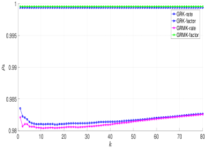
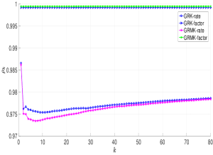
Figure 1: Convergence factors/rates of the GRK and GRMK methods with matrices whose entries are uniformly distributed random numbers between 0 and 1. (left) $A$ is of order $2000\times 200$; (right) $A$ is of order $5000\times 200$. GRK (GRMK)-factor=convergence factor of GRK (GRMK) method; GRK (GRMK)-rate=actual convergence rate of GRK (GRMK) method.

Numerical results show that the convergence factors of the GRMK are indeed a little larger than those of the GRK method. However, the actual convergence rates of the GRMK method are a little smaller than those of the GRK method. In addition, we can also find that the convergence factors are the quite loose upper bounds of the actual convergence rates.

4 The GMBK method

The GMBK method is presented in Algorithm 4. Unlike the GRMK method, after determining the index subset $\mathcal{I}_{k}$, the GMBK method projects the current iterate onto the solution space of this subset simultaneously.

Algorithm 4.

The GMBK method for the systems (1).

1. INPUT:  $A\in R^{m\times n}$, $b\in R^{m}$, $\ell$ , initial estimate $x_{0}$

2. OUTPUT:  $x_{\ell}$

3. For $k=0,1,2,\ldots,\ell-1$ do

4. Compute

   $$\delta_{k}=\frac{1}{2}\left(\max_{1\leq i\leq m}|r^{\left(i\right)}_{k}|^{2}+\sum\limits_{i=1}^{m}\frac{\|A^{(i)}\|_{2}^{2}}{\|A\|_{F}^{2}}|r^{\left(i\right)}_{k}|^{2}\right).$$

5. Determine the index subset of positive integers

   $$\mathcal{I}_{k}=\left\{i_{k}\Bigg{|}|r^{\left(i_{k}\right)}_{k}|^{2}\geq\delta_{k}\right\}.$$

6. Set

   $$x_{k+1}=x_{k}+A_{\mathcal{I}_{k}}^{\dagger}(b_{\mathcal{I}_{k}}-A_{\mathcal{I}_{k}}x_{k}).$$

7. End for

Remark 4.1.

In the GMBK method, we adopt the iterative format (3) to update the approximation. We can also update it in the form of the formula (4) to avoid computing the pseudoinverse.

Remark 4.2.

Similar to Algorithm 2, i.e., the GBK method, we can set the quantity $\delta_{k}$ in Algorithm 4 in the following form

$$\delta_{k}=\xi\max_{1\leq i\leq m}|r^{\left(i\right)}_{k}|^{2},$$

where $\xi\in(0,1]$ is a parameter.

Next, we bound the rate of convergence for Algorithm 4.

Theorem 4.3.

From an initial guess $x_{0}\in{\rm R(A^{T})}$, the sequence $\{x_{k}\}_{k=0}^{\infty}$ generated by the GMBK method converges linearly to the least-Euclidean-norm solution $x_{\star}=A^{{\dagger}}b$ and

$$\|x_{1}-x_{\star}\|^{2}_{2}\leq(1-|\mathcal{I}_{0}|\frac{\min\limits_{i}\|A^{(i)}\|_{2}^{2}}{\lambda_{\max}(A_{\mathcal{I}_{0}}^{T}A_{\mathcal{I}_{0}})}\frac{\lambda_{\min}(A^{T}A)}{\|A\|_{F}^{2}})\|x_{0}-x_{\star}\|^{2}_{2},$$ (15)

and

$$\|x_{k+1}-x_{\star}\|^{2}_{2}\leq(1-\frac{1}{2}|\mathcal{I}_{k}|\frac{\min\limits_{i\notin\mathcal{I}_{k-1}}\|A^{(i)}\|_{2}^{2}}{\lambda_{\max}(A_{\mathcal{I}_{k}}^{T}A_{\mathcal{I}_{k}})}\frac{\lambda_{\min}(A^{T}A)}{\|A\|_{F}^{2}}(\frac{\|A\|_{F}^{2}}{{\|A\|_{F}^{2}-\left\|A_{\mathcal{I}_{k-1}}\right\|_{F}^{2}}}+1))\|x_{k}-x_{\star}\|^{2}_{2},$$

$$\quad k=1,2,\ldots.$$ (16)

Proof 4.4.

From Algorithm 4, using the fact $Ax_{\star}=b$, we have

$$x_{k+1}-x_{\star} = x_{k}-x_{\star}+A_{\mathcal{I}_{k}}^{\dagger}(b_{\mathcal{I}_{k}}-A_{\mathcal{I}_{k}}x_{k})$$

$$= x_{k}-x_{\star}-A_{\mathcal{I}_{k}}^{\dagger}A_{\mathcal{I}_{k}}(x_{k}-x_{\star})$$

$$= (I-A_{\mathcal{I}_{k}}^{\dagger}A_{\mathcal{I}_{k}})(x_{k}-x_{\star}).$$

Since $A_{\mathcal{I}_{k}}^{\dagger}A_{\mathcal{I}_{k}}$ is an orthogonal projector, taking the square of the Euclidean norm on both sides and applying Pythagorean theorem, we get

$$\|x_{k+1}-x_{\star}\|^{2}_{2} =\|(I-A_{\mathcal{I}_{k}}^{\dagger}A_{\mathcal{I}_{k}})(x_{k}-x_{\star})\|^{2}_{2}$$

$$=\|x_{k}-x_{\star}\|^{2}_{2}-\|A_{\mathcal{I}_{k}}^{\dagger}A_{\mathcal{I}_{k}}(x_{k}-x_{\star})\|^{2}_{2},$$

which together with Lemma 2.1 and the fact $\lambda_{\min}((A_{\mathcal{I}_{k}}^{\dagger})^{T}A_{\mathcal{I}_{k}}^{\dagger})=\lambda_{\max}^{-1}(A_{\mathcal{I}_{k}}^{T}A_{\mathcal{I}_{k}})$ yields

$$\|x_{k+1}-x_{\star}\|^{2}_{2} \leq\|x_{k}-x_{\star}\|^{2}_{2}-\lambda_{\min}((A_{\mathcal{I}_{k}}^{\dagger})^{T}A_{\mathcal{I}_{k}}^{\dagger})\|A_{\mathcal{I}_{k}}(x_{k}-x_{\star})\|^{2}_{2}$$

$$=\|x_{k}-x_{\star}\|^{2}_{2}-\lambda_{\max}^{-1}(A_{\mathcal{I}_{k}}^{T}A_{\mathcal{I}_{k}})\|A_{\mathcal{I}_{k}}(x_{k}-x_{\star})\|^{2}_{2}$$

$$=\|x_{k}-x_{\star}\|^{2}_{2}-\lambda_{\max}^{-1}(A_{\mathcal{I}_{k}}^{T}A_{\mathcal{I}_{k}})\sum\limits_{i_{k}\in\mathcal{I}_{k}}|r^{\left(i_{k}\right)}_{k}|^{2}.$$ (17)

Now, the main task is to find the lower bound of $|r^{\left(i_{k}\right)}_{k}|^{2}$.

For $k=0$, substituting (9) into (17), we quickly obtain

$$\|x_{1}-x_{\star}\|^{2}_{2} \leq\|x_{0}-x_{\star}\|^{2}_{2}-\lambda_{\max}^{-1}(A_{\mathcal{I}_{0}}^{T}A_{\mathcal{I}_{0}})|\mathcal{I}_{0}|\frac{\min\limits_{i}\|A^{(i)}\|_{2}^{2}\lambda_{\min}(A^{T}A)}{\|A\|_{F}^{2}}\|x_{0}-x_{\star}\|^{2}_{2}$$

$$\leq(1-|\mathcal{I}_{0}|\frac{\min\limits_{i}\|A^{(i)}\|_{2}^{2}}{\lambda_{\max}(A_{\mathcal{I}_{0}}^{T}A_{\mathcal{I}_{0}})}\frac{\lambda_{\min}(A^{T}A)}{\|A\|_{F}^{2}})\|x_{0}-x_{\star}\|^{2}_{2},$$

which is just the estimate (15).

For $k\geq 1$, similar to the derivation of the inequality (11), we obtain

$$|r^{\left(i_{k}\right)}_{k}|^{2} \geq\frac{1}{2}\frac{\min\limits_{i\notin\mathcal{I}_{k-1}}\|A^{(i)}\|_{2}^{2}\lambda_{\min}(A^{T}A)}{\|A\|_{F}^{2}}(\frac{\|A\|_{F}^{2}}{\sum\limits_{i=1,i\notin\mathcal{I}_{k-1}}^{m}\|A^{(i)}\|_{2}^{2}}+1)\|x_{k}-x_{\star}\|^{2}_{2}$$

$$=\frac{1}{2}\frac{\min\limits_{i\notin\mathcal{I}_{k-1}}\|A^{(i)}\|_{2}^{2}\lambda_{\min}(A^{T}A)}{\|A\|_{F}^{2}}(\frac{\|A\|_{F}^{2}}{\|A\|_{F}^{2}-\left\|A_{\mathcal{I}_{k-1}}\right\|_{F}^{2}}+1)\|x_{k}-x_{\star}\|^{2}_{2}.$$ (18)

Then, substituting (18) into (17), we get

$$\|x_{k+1}-x_{\star}\|^{2}_{2} \leq\|x_{k}-x_{\star}\|^{2}_{2}-\frac{1}{2}|\mathcal{I}_{k}|\frac{\min\limits_{i\notin\mathcal{I}_{k-1}}\|A^{(i)}\|_{2}^{2}}{\lambda_{\max}(A_{\mathcal{I}_{k}}^{T}A_{\mathcal{I}_{k}})}\frac{\lambda_{\min}(A^{T}A)}{\|A\|_{F}^{2}}(\frac{\|A\|_{F}^{2}}{\|A\|_{F}^{2}-\left\|A_{\mathcal{I}_{k-1}}\right\|_{F}^{2}}+1)\|x_{k}-x_{\star}\|^{2}_{2}$$

$$=(1-\frac{1}{2}|\mathcal{I}_{k}|\frac{\min\limits_{i\notin\mathcal{I}_{k-1}}\|A^{(i)}\|_{2}^{2}}{\lambda_{\max}(A_{\mathcal{I}_{k}}^{T}A_{\mathcal{I}_{k}})}\frac{\lambda_{\min}(A^{T}A)}{\|A\|_{F}^{2}}(\frac{\|A\|_{F}^{2}}{\|A\|_{F}^{2}-\left\|A_{\mathcal{I}_{k-1}}\right\|_{F}^{2}}+1)\|x_{k}-x_{\star}\|^{2}_{2},$$

which implies the desired result (16).

Remark 4.5.

From Algorithms 3 and 4, we know that $\{x|A_{\mathcal{I}_{k}}x=b_{\mathcal{I}_{k}}\}\subset\{x|A^{(i_{k})}x=b^{(i_{k})}\}$, where $i_{k}$ is the update index of the GRMK method. Thus, similar to the analysis in ²³, we can obtain

$$\|x_{k}^{GRMK}-x_{k-1}\|^{2}_{2}\leq\|x_{k}^{GMBK}-x_{k-1}\|^{2}_{2},$$

which together with the fact

$$\left\|{x}_{k}^{GRMK}-{x}_{k-1}\right\|^{2}_{2}+\left\|{x}_{k}^{GRMK}-{x}_{\star}\right\|^{2}_{2} =\left\|{x}_{k-1}-{x}_{\star}\right\|^{2}_{2}$$

$$=\left\|{x}_{k}^{GMBK}-{x}_{k-1}\right\|^{2}_{2}+\left\|{x}_{k}^{GMBK}-{x}_{\star}\right\|^{2}_{2},$$

leads to

$$\|x_{k}^{GMBK}-x_{\star}\|^{2}_{2}\leq\|x_{k}^{GRMK}-x_{\star}\|^{2}_{2}.$$

In the above expressions, $x_{k}^{GMBK}$ and $x_{k}^{GRMK}$ denote the next approximations generated by the GMBK and GRMK methods, respectively. Hence, the GMBK method converges at least as fast as the GRMK method.

In addition, since $\{x|A_{\mathcal{I}_{k}}x=b_{\mathcal{I}_{k}}\}\subset\{x|A^{(l_{k})}x=b^{(l_{k})}\}$, where $l_{k}={\rm arg}\max\limits_{1\leq i\leq m}|r^{\left(i\right)}_{k}|^{2}$, we can also get that the GMBK method must converge at least as fast as the Motzkin method.

Remark 4.6.

To compare Algorithms 2 and 4 fairly, in the following, we set $\eta$ in Algorithm 2 to be

$$\eta=\frac{1}{2}+\frac{1}{2}\frac{\left\|b-Ax_{k}\right\|_{2}^{2}}{\|A\|_{F}^{2}}\left(\max_{1\leq i_{k}\leq m}\left\{\frac{\left|b^{i_{k}}-A^{(i_{k})}x_{k}\right|^{2}}{\left\|A^{(i_{k})}\right\|_{2}^{2}}\right\}\right)^{-1},$$

that is, set

$$\epsilon_{k}=\frac{1}{2}\left(\max_{1\leq i_{k}\leq m}\left\{\frac{|r^{\left(i_{k}\right)}_{k}|^{2}}{\left\|A^{\left(i_{k}\right)}\right\|_{2}^{2}}\right\}+\frac{\left\|r_{k}\right\|_{2}^{2}}{\|A\|_{F}^{2}}\right).$$

We refer to this block algorithm as the greedy distance block Kaczmarz (GDBK) method.

From Remark 3.6, we know that the convergence factor cannot accurately explain the convergence speed of a method. So, we compare the actual convergence rates defined in (14) of the GDBK and GMBK methods using numerical experiments. The numerical results are listed in Fig. 2, which show that these actual convergence rates are almost the same.

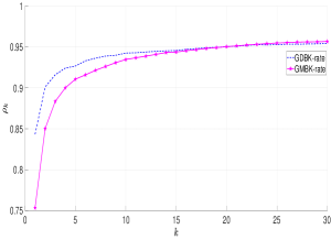
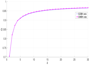
Figure 2: Actual convergence rates of the GDBK and GMBK methods with matrices whose entries are uniformly distributed random numbers between 0 and 1. (left) $A$ is of order $1000\times 200$; (right) $A$ is of order $5000\times 1000$. GDBK (GMBK)-rate=actual convergence rate of GDBK (GMBK) method.

5 Numerical experiments

In this section, we mainly compare our new greedy Motzkin-Kaczmarz methods (GRMK, GMBK) with the greedy distance Kaczmarz methods (GRK, GDBK) in terms of the iteration numbers (denoted as “Iteration”) and computing time in seconds (denoted as “CPU time(s)”) with different matrices $A\in R^{m\times n}$. In all the following specific experiments, we generate the solution vector $x_{\star}\in R^{n}$ using the MATLAB function randn, and the vector $b\in R^{m}$ by setting $b=Ax_{\star}$. All experiments start from an initial vector $x_{0}=0$, and terminate once the relative solution error (RES) or relative residual (RR) at $x_{k}$ is less than $10^{-10}$, where RES and RR are defined by

$$\rm RES=\frac{\left\|x_{k}-A^{\dagger}b\right\|^{2}_{2}}{\left\|A^{\dagger}b\right\|^{2}_{2}},~{}~{}\mathrm{RR}=\frac{\left\|b-Ax_{k}\right\|_{2}^{2}}{\left\|b-Ax_{0}\right\|_{2}^{2}}.$$

We first consider three main models of the coefficient matrix $A$: a Gaussian matrix with i.i.d. $N(0,1)$ entries generated by the MATLAB function randn, a sparse normally distributed random matrix generated by the MATLAB function sprandn(m,n,0.2,0.8), and a sparse uniformly distributed random matrix generated by the MATLAB function sprand(m,n,0.2,0.8). Numerical results are reported in Figures 3–8, which describe the $\log_{10}$(RES) or $\log_{10}$(RR) against the iteration number and CPU time. From these figures, we can find that for dense matrices, i.e., the matrices with i.i.d. $N(0,1)$ entries, the performances of the GRMK and GRK methods are almost the same; for sparse matrices, the GRMK method outperforms the GRK method in CPU time; for all the cases, the GMBK and GDBK methods have almost the same performance.

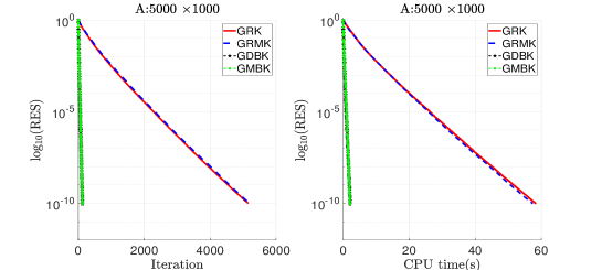
Figure 3: Performance of the methods on $A\in R^{5000\times 1000}$ with i.i.d. $N(0,1)$ entries.

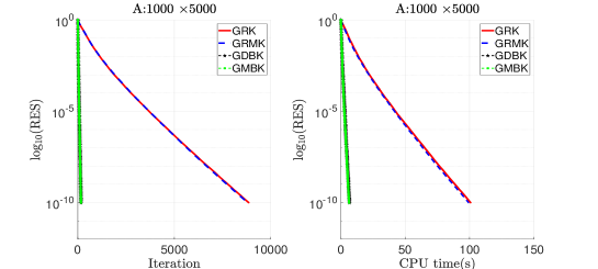
Figure 4: Performance of the methods on $A\in R^{1000\times 5000}$ with i.i.d. $N(0,1)$ entries.

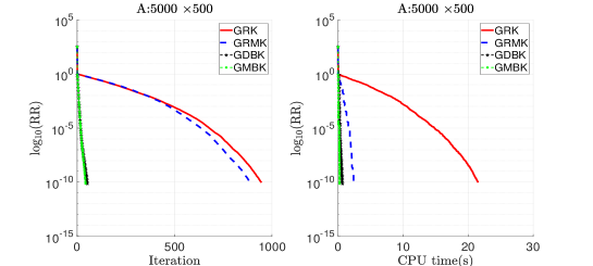
Figure 5: Performance of the methods on $A$ generated by the MATLAB function sprandn(5000,500,0.2,0.8).

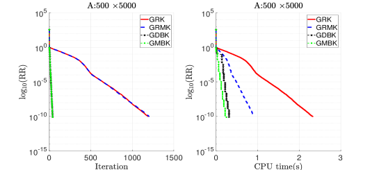
Figure 6: Performance of the methods on $A$ generated by the MATLAB function sprandn(500,5000,0.2,0.8).

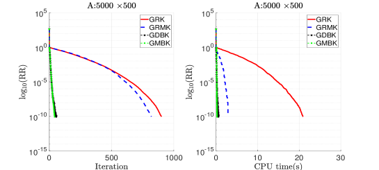
Figure 7: Performance of the methods on $A$ generated by the MATLAB function sprand(5000,500,0.2,0.8).

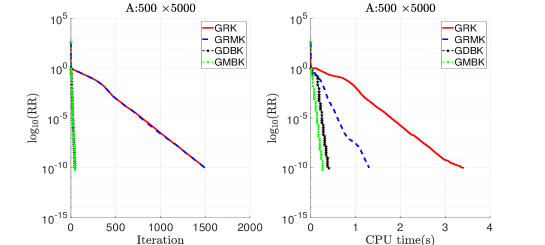
Figure 8: Performance of the methods on $A$ generated by the MATLAB function sprand(500,5000,0.2,0.8).

We also compare the performance of the methods on a real-world matrix, mk9-b3, taken from ³⁶. Numerical results are reported in Figures 9–10, which show the similar results obtained from the above experiments on dense matrices. That is, the GRMK method and its block version have almost the same performance as the GRK method and its block version.

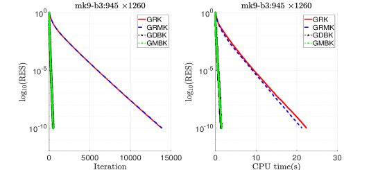
Figure 9: Performance of the methods on a real-world matrix, mk9-b3 ($945\times 1260$).

Figure 10: Performance of the methods on a real-world matrix, mk9-b3 ($945\times 1260$).

References

• 1 Kaczmarz S. Angenäherte Auflösung von Systemen linearer Gleichungen. Bull Int Acad Pol Sci Lett A. 1937;35:355–357.
• 2 Strohmer T, and Vershynin R. A randomized Kaczmarz algorithm with exponential convergence. J Fourier Anal Appl. 2009;15:262–278.
• 3 Needell D. Randomized Kaczmarz solver for noisy linear systems. BIT Numer Math. 2010;50:395–403.
• 4 Zouzias A, and Freris MN. Randomized extended Kaczmarz for solving least squares. SIAM J Matrix Anal Appl. 2013;34:773–793.
• 5 Ma A, Needell D, and Ramdas A. Convergence properties of the randomized extended Gauss–Seidel and Kaczmarz methods. SIAM J Matrix Anal Appl. 2015;36:1590–1604.
• 6 Du K. Tight upper bounds for the convergence of the randomized extended Kaczmarz and Gauss–Seidel algorithms. Numer Linear Algebra Appl. 2019;26(3):e2233.
• 7 Bai ZZ, and Wu WT. On greedy randomized Kaczmarz method for solving large sparse linear systems. SIAM J Sci Comput. 2018;40(1):A592–A606.
• 8 Bai ZZ, and Wu WT. On relaxed greedy randomized Kaczmarz methods for solving large sparse linear systems. Appl Math Lett. 2018;83:21–26.
• 9 Zhang JJ. A new greedy Kaczmarz algorithm for the solution of very large linear systems. Appl Math Lett. 2019;91:207–212.
• 10 Huang X, Liu G, and Niu Q. Remarks on Kaczmarz algorithm for solving consistent and inconsistent system of linear equations. In: International Conference on Computational Science. Springer; 2020. p. 225–236.
• 11 Bai ZZ, and Wu WT. On greedy randomized coordinate descent methods for solving large linear least-squares problems. Numer Linear Algebra Appl. 2019;26(4):1–15.
• 12 Zhang JH, and Guo JH. On relaxed greedy randomized coordinate descent methods for solving large linear least-squares problems. Appl Numer Math. 2020;157:372–384.
• 13 Liu Y, and Gu CQ. Variant of greedy randomized Kaczmarz for ridge regression. Appl Numer Math. 2019;143:223–246.
• 14 Eldar Y, and Needell D. Acceleration of randomized Kaczmarz method via the Johnson-Lindenstrauss lemma. Numer Algor. 2011;58:163–177.
• 15 Du K, and Gao H. A new theoretical estimate for the convergence rate of the maximal weighted residual Kaczmarz algorithm. Numer Math Theor Meth Appl. 2019;12(2):627–639.
• 16 Nutini J, Sepehry B, Laradji I, Schmidt M, Koepke H, and Virani A. Convergence rates for greedy Kaczmarz algorithms, and faster randomized Kaczmarz rules using the orthogonality graph. arXiv preprint arXiv:161207838; 2016.
• 17 Griebel M, and Oswald P. Greedy and randomized versions of the multiplicative Schwarz method. Linear Algebra Appl. 2012;437(7):1596–1610.
• 18 Agamon S. The relaxation method for linear inequalities. Canad J Math. 1954;6:382–392.
• 19 Motzkin TS, and Schoenberg IJ. The relaxation method for linear inequalities. Canad J Math. 1954;6:393–404.
• 20 Petra S, and Popa C. Single projection Kaczmarz extended algorithms. Numer Algor. 2016;73:791–806.
• 21 De Loera JA, Haddock J, and Needell D. A sampling Kaczmarz–Motzkin algorithm for linear feasibility. SIAM J Sci Comput. 2017;39(5):S66–S87.
• 22 Haddock J, and Needell D. On Motzkin’s method for inconsistent linear systems. BIT Numer Math. 2019;59(2):387–401.
• 23 Haddock J, and Ma A. Greed works: an improved analysis of sampling Kaczmarz–Motzkin. arXiv preprint arXiv:1912.03544; 2019.
• 24 Rebrova E, and Needell D. Sketching for Motzkin’s iterative method for linear systems. Proc. 50th Asilomar Conf. on Signals, Systems and Computers; 2019.
• 25 Morshed MS, Islam MS, and Noor-E-Alam M. Accelerated sampling Kaczmarz Motzkin algorithm for the linear feasibility problem. J Global Optim. 2020;77(2):361–382.
• 26 Morshed MS, and Noor-E-Alam M. Heavy ball momentum induced sampling Kaczmarz Motzkin methods for linear feasibility problems. arXiv preprint arXiv:200908251; 2020.
• 27 Needell D, and Tropp JA. Paved with good intentions: analysis of a randomized block Kaczmarz method. Linear Algebra Appl. 2014;441:199–221.
• 28 Needell D, Zhao R, and Zouzias A. Randomized block Kaczmarz method with projection for solving least squares. Linear Algebra Appl. 2015;484:322–343.
• 29 Gower RM, and Richtárik P. Randomized iterative methods for linear systems. SIAM J Matrix Anal Appl. 2015;36(4):1660–1690.
• 30 Briskman J, and Needell D. Block Kaczmarz method with inequalities. JMathImaging Vision. 2015;52(3):385–396.
• 31 Necoara I. Faster randomized block Kaczmarz algorithms. SIAM J Matrix Anal Appl. 2019;40:1425–1452.
• 32 Du K, Si WT, and Sun XH. Pseudoinverse–free randomized extended block Kaczmarz for solving least squares. arXiv preprint arXiv:2001.04179; 2020.
• 33 Moorman JD, Tu TK, Molitor D, and Needell D. Randomized Kaczmarz with averaging. BIT Numer. Math.; 2020.
• 34 Niu YQ, and Zheng B. A greedy block Kaczmarz algorithm for solving large–scale linear systems. Appl Math Lett. 2020;104:106294.
• 35 Li HY, and Zhang YJ. A novel greedy Kaczmarz method for solving consistent linear systems. arXiv preprint arXiv:200402062; 2020.
• 36 Davis TA, and Hu YF. The university of florida sparse matrix collection. ACM Trans Math Softw. 2011;38(1):1–25.