Discrete Cosine Transform Based Causal Convolutional Neural Network for Drift Compensation in Chemical Sensors

Abstract

Sensor drift is a major problem in chemical sensors that requires addressing for reliable and accurate detection of chemical analytes. In this paper, we develop a causal convolutional neural network (CNN) with a Discrete Cosine Transform (DCT) layer to estimate the drift signal. In the DCT module, we apply soft-thresholding nonlinearity in the transform domain to denoise the data and obtain a sparse representation of the drift signal. The soft-threshold values are learned during training. Our results show that DCT layer-based CNNs are able to produce a slowly varying baseline drift signal. We train the CNN on synthetic data and test it on real chemical sensor data. Our results show that we can have an accurate and smooth drift estimate even when the observed sensor signal is very noisy.

Index Terms—  chemical sensor drift, chemical sensor, time series analysis, discrete cosine transform, convolutional neural networks

1 Introduction

Chemical sensors have been used for detecting and identifying chemical analytes in a wide array of industrial and safety applications[1]. Despite the fact that chemical sensor technology provides practical solutions, sensor responses may degrade with time, resulting in inconsistent results.This phenomenon is known as sensor drift. Sensor drift arises because of internal factors such as sensor poisoning and aging, and/or external factors such as humidity and temperature changes [2]. The chemical sensory system becomes unreliable over time, if the sensor drift signal is not properly estimated.

There has been extensive work to address the drift problem using signal processing and machine learning. One common approach is to extract features carefully from the time series sensor measurements and optimize a machine learning algorithm to recognize patterns from these features [3, 4]. In [3], discriminative features are extracted from the responses of the sensors and then fed into support vector machines to identify the gas analyte identity. Others have employed different methods to counteract the sensor drift for the task of analyte identification, such as domain adaptation [5, 6], semi-supervised learning [7], and deep stacked autoencoders [8]. In the aforementioned papers, the features extracted from the sensors become unreliable as the sensor ages. On the other hand, other approaches try to estimate the drift directly from the time-series measurements of the sensors using iterative interpolation techniques [9], or by using Independent Component Analysis [10]. After the drift signal is estimated, it can be subtracted from the sensor measurements to determine the actual sensor response.

The wide success of deep convolutional neural networks (CNNs) has been demonstrated by their ability to achieve state-of-the-art performance in many time-series recognition tasks. CNNs have been used in analyte classification problems [11, 4]. One particular variant of convolutional neural networks, the temporal convolutional neural network (TCNN), has been shown to outperform recurrent neural networks on many benchmark data sets [12, 13]. This motivates us to employ a TCNN-based framework to address the problem of drift correction in chemical sensor data. Given the fact that sensor drift is a slowly varying signal, we propose utilizing the Discrete Cosine Transform (DCT) to extract a baseline drift signal from the observed sensor signal. In particular, we propose a new type of layer to be integrated into the conventional TCNN, which we call DCT-based sub-network. In the DCT-based sub-network, we compute the DCT over sliding short-time windows of the temporal feature maps. We then apply the soft-thresholding nonlinearity in the transform domain and compute the inverse DCT to transform the features back to time domain. In the transform domain, we use soft-thresholding that is parametrized by threshold variables, which are learned during training by the standard backpropagation algorithm. Our results show that the the nonlinear denoising and smoothing in transform domain using the DCT-based structure removes the high-frequency features, i.e., induces smoothness in the features and, subsequently, the constructed output baseline drift signal. Any significant deviation from the sensor baseline signal indicates the existence of chemical vapors.

The organization of this paper is as follows: First we explain the drift problem, TCNN-framework and the DCT-based structure for drift estimation in Section 2. In Section 3, we present experimental results. Finally, in Section 4 we conclude our work.

2 Causal DCT-based Real-Time Sensor Drift Estimation Framework

The drift response of ChemFET sensors is modeled as a linear combination of exponential decays [14, 15, 16, 17, 18]. In our ChemFET sensors we can approximate the drift waveform using the following model [19, 20]:

$$d(t)=(R_{0}+\epsilon_{R})+R_{f}\ \text{exp}\Big{(}\frac{-t}{\tau_{f}+\epsilon_{f}}\Big{)}+R_{s}\ \text{exp}\Big{(}\frac{-t}{\tau_{s}+\epsilon_{s}}\Big{)}$$ (1)

where $R(0)=R_{0}+\epsilon_{R}+R_{f}+R_{s}$ is the sensor conversion factor at the initial time after deployment and reset, $R_{f}$, $R_{s}$ are fast and slow drift coefficients, $\tau_{f}$, $\tau_{s}$ are fast and slow drift time constants, and $\epsilon_{R}$, $\epsilon_{f}$, $\epsilon_{s}$ are the corresponding error terms for each of the model variables. It is not possible to know the values of the time constants and other parameters in Eq. 1 but this model enables us to generate a random population of sensors with individual sensitivities and individual time constants that can differ significantly.

Let a sensor time measurement be $y(t)$ at time $t$. Let $d(t)$ be the drift signal at time $t$. Let $p(t)$ be the desired sensor response without the drift component (drift-corrected response in absence of noise). The observed sensor measurement is $y(t)=d(t)+p(t)+v(t)$, where $v(t)$ is the noise signal. Given $y(t)$, we are interested in estimating the drift signal $d(t)$ so that we can estimate $p(t)$.

When a sensor is exposed to a gas vapour, it starts absorbing the vapour and its response changes accordingly. Once the sensor is no longer exposed to the gas vapour, it starts exuding the vapour it had absorbed earlier. Absorbing and exuding the vapour depends on the sensor material, the analyte type and the environment. The ideal sensor response in the absence of drift can be approximated analytically as follows [21],:

where $T_{s}$ is the starting time of the exposure, and $\Delta T$ is the exposure duration. When the sensors are not exposed to any chemical analytes, the response will be simply $y(t)=d(t)+v(t)$. Therefore, we can consider estimating the drift as a baseline (background) estimation problem. An example is shown in Fig 1 in which the sensor is exposed to Volatile Organic Compounds (VOC) three times (the blue curve). Since the drift waveform is decaying, it is not possible to set a threshold without estimating the drift waveform to detect the gas.

In [9], the drift estimation is posed as a missing data interpolation problem and the Papoulis-Gerchberg (PG) method is used. The PG method is an iterative method involving sequential forward and inverse Fourier Transform computations over blocks of sensor data. It requires some time-domain information about the drift signal and it is assumed that the sensor is not exposed to gas vapor initially. To interpolate the “missing” drift portions where $p(t)\neq 0$, the authors also assumed a low-pass bandwidth (BW) for the drift signal in the Fourier domain [9]. In contrast, we do not assume any prior bandwidth information. The neural network automatically imposes the sparsity constraint on the drift signal in the transform domain during training by learning DCT domain soft thresholds. Furthermore, we do not use future samples during the DCT computation to estimate the drift signal $d(t)$. We use only the past and current samples of $y(t)$ to estimate the drift signal $d(t)$. As a result, we compute a real-time estimate of $d(t)$.

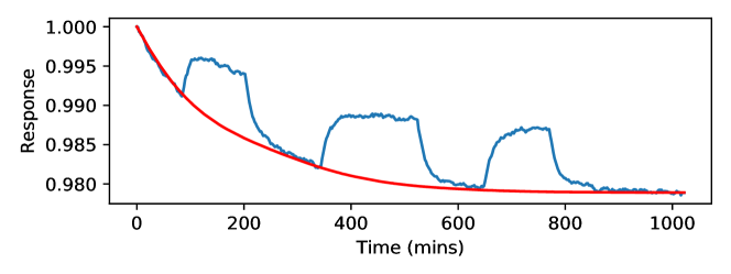
Fig. 1: Overall sensor measurement signal (blue) and the underlying drift signal (red)

2.1 TCNN with a DCT layer

We developed a Temporal Convolutional Neural Network (TCNN) with a DCT layer to extract the drift signal $d[n]$ from the observed sensor signal $y[n]$. In TCNN, the convolutional layers implement causal convolution. Therefore, in this approach, given a time series $y[t]$ for $t=\{1,2,\ ...\ n\}$, one can determine a drift estimate $\hat{d}[n]$ and, subsequently, $\hat{p}[n]=y[n]-\hat{d}[n]$ . TCNN implements the so-called dilated convolution in their convolutional layers, which can be expressed as $y_{r}[n]:=\sum_{k=0}^{K-1}h[k]x[n-rk],$ where $h$ is the 1-d temporal filter of length $K$, and $r$ is the dilation rate.

TCNN is made up of successive convolutional blocks, for which the dilation rate of the convolution is increased exponentially as we go up. Furthermore, residual connections are also used between successive blocks of convolutional layers. This is particularly useful for our task given that the drift signal is a low frequency signal. On the other hand an exposure to a gas analyte vapor will result in a sudden increase in the recorded sensor signal value $y[n]$.

Our TCN design goes as follows: We first apply an ordinary convolutional layer with filters of length 5. Afterwards, we apply convolutional blocks with dilated convolution and residual connections. Each of the convolutional blocks comprises two dilated convolutional layers with a spatial dropout layer in between. The second layer in each block has residual connections with the output of the previous block. The dilation rate increases by 2 from $r=2$ in the first dilated convolutional block to $r=2^{7}=128$ in the last dilated convolutional block. The number of feature maps is 64 throughout all the layers. The spatial dropout rate is set to 0.2. Afterwards, we feed the 64 feature maps of the last layer of TCNN module into the DCT layer, in which we carry out the transform domain processing as explained in Sec. 3. The DCT window size is set to 64. Finally, we apply a $1\times 1$ convolution without any nonlinearity to estimate the drift signal $d[n]$. The DCT domain processing is described in Subsection 2.2 in detail.

The whole framework is trained to minimize the following cost function:

$$\begin{split}\mathcal{J}:=&\sum_{n=0}^{N-1}\big{(}d[n]-\hat{d}[n]\big{)}^{2}+\lambda\sum_{n=1}^{N-1}|\hat{d}[n]-\hat{d}[n-1]|,\end{split}$$ (3)

where the first term in the cost criterion is the reconstruction square errors. The second term is the Total Variation (TV) regularization term.
2.2 DCT-based Layers

Discrete cosine transform has been widely used in image compression and speech coding. In this work, we propose incorporating DCT in the TCNN framework to construct smooth drift estimates from the observed signal $y[n]$. In particular, let $f_{i}[n]$ be the i-th feature arising from the TCNN at time instance $n$. The DCT coefficients over a sliding windows of size $N$ are given by:

$$F_{n,i}(k):=\sum_{l=0}^{N-1}f^{i}[n-l]\text{cos}\Big{(}\frac{\pi k}{N}(N-l+\frac{1}{2})\Big{)},$$ (4)

where $k\in\{0,1,...,N-1\}$ is the DCT index, and ${F}_{n,i}$ is the transform of the feature segment $f_{i}[t]\ \text{for}\ t\in\{n-N+1,...,n\}$.

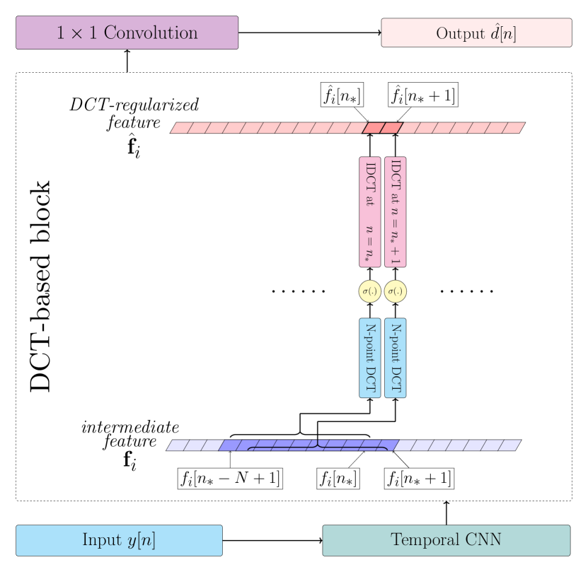
Fig. 2: Block diagram of the DCT-based NN structure. The non-linearity $\sigma(.)$ represents to the soft-thresholding function.

After the DCT computation we apply sign-preserving soft-thresholding nonlinearity in the transform domain. For this purpose, we use the soft thresholding function defined for a scalar input $x$ as $\texttt{SoftTh}(x):=\text{sgn}(x)\text{max}(0,|x|-b)$. The threshold $b\geq 0$ is analogous to the additive bias term in regular time-domain convolutional layers. The parameter $b$ is learned during training by standard backpropagation. The soft-thresholding function $\texttt{SoftTh}(.)$ is applied element-wise to the coefficients ${F}_{n,i}(k)$. Each feature map $f_{i}$ will have an associated thresholding parameter $b_{i}$. This proposed soft-thresholding also induces sparsity in the spectral representation. After thresholding we transform back to the time (feature) domain using the inverse discrete cosine transform (IDCT) and realize a smoothed feature point $\hat{f}_{i}[n]$. Notice that, for each feature map, we only need to evaluate IDCT for one single point at time $n$, that is the smoothed version of the original feature value at time $n$. The DCT based TCNN structure is shown in Fig. 2.

Metric	Bandwidth used in the PG Algorithm $(\times\frac{2\pi}{4096})$												TCNN-DCT
	5	6	7	8	9	10	11	12	13	14	15	16
MSE (avg.)	1.47	0.91	0.79	1.23	1.34	1.16	0.99	0.86	1.03	1.25	1.54	1.70	0.05
MSE (median)	0.28	0.10	0.23	0.22	0.20	0.16	0.16	0.17	0.27	0.33	0.37	0.55	0.02
Cos sim (avg.)	0.81	0.87	0.89	0.77	0.74	0.83	0.87	0.89	0.85	0.82	0.79	0.72	0.97
Cos sim (median)	0.94	0.95	0.92	0.87	0.89	0.92	0.93	0.93	0.88	0.85	0.80	0.74	0.99

Table 1: Comparison of TCNN-DCT framework vs the PG algorithm over the 5,000 examples in the validation data set. We implemented the PG algorithm with different bandwidth values. We report the results for two metrics: MSE (mean square error between the estimate drift and the true drift) and Cos sim (cosine similarity between the estimated drift and the true drift).

3 Experimental Results

In our experiments we used Electronic-nose (E-nose) measurements from the data collected by the JPL [22] using 32 different carbon-polymer sensors for air quality monitoring. We only considered recordings corresponding to single-gas (methanol) exposure experiments as in [9]. Some recording examples are shown in Fig. 3. We also collected our own data using the commercially available MQ-137 ammonia sensor which has detection range of 5-500 ppm. Three typical sensor recordings are shown at the bottom three rows of Fig. 3. We also generated synthetic data for training and validating our network model. The real E-nose data was then used as our test set. All the data are resized to a length of 512.

Sensor	PG Algorithm		TCNN-DCT
	MSE	Cos. sim.	MSE	Cos. sim.
Sensor 1	0.07	0.97	0.04	0.98
Sensor 2	0.03	0.97	0.01	0.99
Sensor 3	0.18	0.99	0.04	0.99
Sensor 4	0.20	0.94	0.12	0.94
Sensor 5	0.04	0.97	0.01	0.99
Sensor 6	0.05	0.89	0.09	0.92

Table 2: Comparison of TCNN-DCT framework vs. the PG algorithm over the real data shown in Fig. 3 (We report the results of only 6 sensors due to the lack of space).

We synthesized 10,000 recordings that resemble idealized sensor responses for different analyte exposure profiles with slowly varying drift to train the CNN. We used Eq. 2 to synthesize sensor responses and we randomized the starting instances of gas vapors, the exposure period, the parameters $\beta$ and $\tau$, and the number of exposure sessions in order to create as diverse a data set as possible. We synthesized the drift signal simply by sampling from a Gaussian process with covariance $\mathbb{E}(x(t_{1})-\mu)(x(t_{2})-\mu)=\text{exp}\big{(}-\big{(}{\frac{t_{1}-t_{2}}{\alpha}}\big{)}^{2}\big{)}$ where $\alpha$ is chosen to be sufficiently large so that the realizations of the drift signal are slowly varying with time. We normalized both the synthetic and real data using global mean and standard deviation. We trained our network using the synthetic training data for 80 epochs. We set the TV parameter $\lambda$ in Eq. 3 to 0.1.

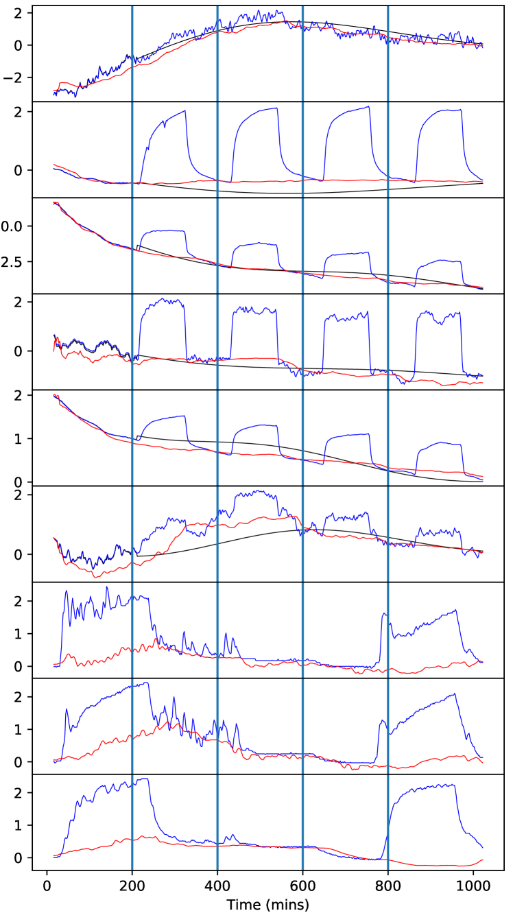
Fig. 3: 9 real sensor data (in blue), the estimated drift using TCN-DCT framework (in red), and the estimated drift using PG algorithm (in dashed black). The first 6 sensors are from Data Set II, while the last three are from our Data Set I. The first (top) and the sixth examples are ”non-informative” (damaged) sensors.

We implemented the Papoulis-Gerchberg (PG) algorithm over the test data set as in [9] to compare it with our approach. We assumed that there is no gas vapor exposure to the sensor initially and at the end of the recording. We extrapolated the remaining part of the drift signal using the PG algorithm. Drift signal estimation results are shown in Fig 3. The proposed TCNN-DCT framework is superior to the PG algorithm in terms of cosine similarity and the MSE as shown in Tables 1 and 2, and Fig. 3. In Table 1, we have a range of bandwidth values for the PG algorithm to get the best possible result and in Table 2 we manually optimized the bandwidth for the PG algorithm. In Fig. 3, the 1st (top) and the 6th sensors are called ”non-informative” (damaged) sensors in [9]. The 1st sensor does not produce any response to the gas exposure. In this case, the estimated drift signal is just a smooth (denoised) version of the sensor signal. In the last three examples, there is almost no drift, and our drift estimate follows the baseline accurately.

Another advantage of our method compared to the PG method is that we do not require any prior knowledge about the sensor signal. In the PG method one has to know a gas vapor free segment of the response to estimate the drift.

4 Conclusion

We proposed a novel deep DCT structure. The DCT layer is integrated into deep CNNs in order to causally estimate the slowly-varying drift signal in chemical sensors from the sensor response to gas vapor exposure. In the DCT layer, we perform soft thresholding before transforming back to time domain. The DCT helps regularize the intermediate features generated by the early layers of the TCNN and this leads to an accurate baseline drift signal. Our network outperforms the PG type sensor drift estimation algorithms without requiring any prior knowledge about the drift signal.

References

- [1] K. Arshak, E. Moore, G. Lyons, J. Harris, and S. Clifford, “A review of gas sensors employed in electronic nose applications,” Sensor review, 2004.
- [2] M. Holmberg, F. Winquist, I. Lundström, F. Davide, C. DiNatale, and A. D’Amico, “Drift counteraction for an electronic nose,” Sensors and Actuators B: Chemical, vol. 36, no. 1-3, pp. 528–535, 1996.
- [3] A. Vergara, S. Vembu, T. Ayhan, M. A. Ryan, M. L. Homer, and R. Huerta, “Chemical gas sensor drift compensation using classifier ensembles,” Sensors and Actuators B: Chemical, vol. 166, pp. 320–329, 2012.
- [4] D. Badawi, T. Ayhan, S. Ozev, C. Yang, A. Orailoglu, and A. E. Cetin, “Detecting gas vapor leaks using uncalibrated sensors,” IEEE Access, vol. 7, pp. 155 701–155 710, 2019.
- [5] Q. Liu, X. Li, M. Ye, S. S. Ge, and X. Du, “Drift compensation for electronic nose by semi-supervised domain adaption,” IEEE Sensors Journal, vol. 14, no. 3, pp. 657–665, 2013.
- [6] L. Zhang and D. Zhang, “Domain adaptation extreme learning machines for drift compensation in e-nose systems,” IEEE Transactions on instrumentation and measurement, vol. 64, no. 7, pp. 1790–1801, 2014.
- [7] S. De Vito, G. Fattoruso, M. Pardo, F. Tortorella, and G. Di Francia, “Semi-supervised learning techniques in artificial olfaction: A novel approach to classification problems and drift counteraction,” IEEE Sensors Journal, vol. 12, no. 11, pp. 3215–3224, 2012.
- [8] Q. Liu, X. Hu, M. Ye, X. Cheng, and F. Li, “Gas recognition under sensor drift by using deep learning,” International Journal of Intelligent Systems, vol. 30, no. 8, pp. 907–922, 2015.
- [9] D. Huang and H. Leung, “Reconstruction of drifting sensor responses based on papoulis–gerchberg method,” IEEE Sensors Journal, vol. 9, no. 5, pp. 595–604, 2009.
- [10] C. Di Natale, E. Martinelli, and A. D’Amico, “Counteraction of environmental disturbances of electronic nose data by independent component analysis,” Sensors and Actuators B: Chemical, vol. 82, no. 2-3, pp. 158–165, 2002.
- [11] P. Peng, X. Zhao, X. Pan, and W. Ye, “Gas classification using deep convolutional neural networks,” Sensors, vol. 18, no. 1, p. 157, 2018.
- [12] S. Bai, J. Z. Kolter, and V. Koltun, “An empirical evaluation of generic convolutional and recurrent networks for sequence modeling,” arXiv preprint arXiv:1803.01271, 2018.
- [13] L. S. Mokatren, A. E. Cetin, and R. Ansari, “Deep layered lms predictor,” arXiv preprint arXiv:1905.04596, 2019.
- [14] D. Chen and P. K. Chan, “An intelligent isfet sensory system with temperature and drift compensation for long-term monitoring,” IEEE Sensors Journal, vol. 8, no. 12, pp. 1948–1959, 2008.
- [15] K.-M. Chang, C.-T. Chang, K.-Y. Chao, and C.-H. Lin, “A novel ph-dependent drift improvement method for zirconium dioxide gated ph-ion sensitive field effect transistors,” Sensors, vol. 10, no. 5, pp. 4643–4654, 2010.
- [16] L. Bousse, N. F. De Rooij, and P. Bergveld, “Operation of chemically sensitive field-effect sensors as a function of the insulator-electrolyte interface,” IEEE Transactions on Electron Devices, vol. 30, no. 10, pp. 1263–1270, 1983.
- [17] C. Z. Goh, P. Georgiou, T. G. Constandinou, T. Prodromakis, and C. Toumazou, “A cmos-based isfet chemical imager with auto-calibration capability,” IEEE Sensors Journal, vol. 11, no. 12, pp. 3253–3260, 2011.
- [18] B. C. Jacquot, N. Munoz, D. W. Branch, and E. C. Kan, “Non-faradaic electrochemical detection of protein interactions by integrated neuromorphic cmos sensors,” Biosensors and Bioelectronics, vol. 23, no. 10, pp. 1503–1511, 2008.
- [19] F. Karabacak, U. Obahiagbon, U. Ogras, S. Ozev, and J. B. Christen, “Making unreliable chem-fet sensors smart via soft calibration,” in 2016 17th International Symposium on Quality Electronic Design (ISQED). IEEE, 2016, pp. 456–461.
- [20] C. Yang, P. Cronin, A. Agambayev, S. Ozev, A. E. Cetin, and A. Orailoglu, “A crowd-based explosive detection system with two-level feedback sensor calibration,” in ICCAD, 2020.
- [21] L. Carmel, S. Levy, D. Lancet, and D. Harel, “A feature extraction method for chemical sensors in electronic noses,” Sensors and Actuators B: Chemical, vol. 93, no. 1-3, pp. 67–76, 2003.
- [22] H. Zhou, M. L. Homer, A. V. Shevade, and M. A. Ryan, “Nonlinear least-squares based method for identifying and quantifying single and mixed contaminants in air with an electronic nose,” Sensors, vol. 6, no. 1, pp. 1–18, 2006.