Mean perimeter and area of the convex hull of a planar Brownian motion in the presence of resetting

Abstract

We compute exactly the mean perimeter and the mean area of the convex hull of a $2$-d Brownian motion of duration $t$ and diffusion constant $D$, in the presence of resetting to the origin at a constant rate $r$. We show that for any $t$, the mean perimeter is given by $\langle L(t)\rangle=2\pi\sqrt{\frac{D}{r}}\,f_{1}(rt)$ and the mean area is given by $\langle A(t)\rangle=2\pi\frac{D}{r}\,f_{2}(rt)$ where the scaling functions $f_{1}(z)$ and $f_{2}(z)$ are computed explicitly. For large $t\gg 1/r$, the mean perimeter grows extremely slowly as $\langle L(t)\rangle\propto\ln(rt)$ with time. Likewise, the mean area also grows slowly as $\langle A(t)\rangle\propto\ln^{2}(rt)$ for $t\gg 1/r$. Our exact results indicate that the convex hull, in the presence of resetting, approaches a circular shape at late times. Numerical simulations are in perfect agreement with our analytical predictions.

I Introduction

Stochastic processes with resetting have recently emerged as a very active area of research in statistical physics, due to its numerous applications spanning across interdisciplinary fields ranging from ecology to computer science – for a recent review see Reset_review . The main idea behind resetting is very simple. When one is searching for a hidden item, using randomised search algorithms (e.g. diffusive search for food by animals during their foraging period), it is often advantageous to interrupt the process stochastically at a constant $r$ and restart the dynamics from the initial position. The effect of resetting has been demonstrated in a wide variety of problems: diffusive processes such as Brownian motion EM2011.1 ; EM2011.2 ; WEM2013 ; MV2013 ; EM2014 ; MSS2015 ; PKE2016 ; BBR2016 ; Pal2015 ; PR2017 ; Reuveni_16 , random walks and Lévy flights KMSS2014 ; KG2015 , random acceleration process Singh2020 , active particles EM2018 ; Masoliver2019 ; KSB2020 , enzymatic reactions RUK2014 ; Reuveni_16 , foraging ecology BS2014 ; GGC2019 , active transport in living cells Bres2020 . Various resetting protocols, some going beyond the canonical Poissonian resetting, have also been studied MSS2015_1 ; Besga2020 ; NG16 ; Shkilev17 ; somrita ; Bruyne2020 ; CS15 ; BEM2017 ; FBGM2017 ; CS2018 ; BFGM2019 ; MBMS2020 ; GPKP2020 ; Bres2020_1 ; Bres2020_2 . Another interesting feature of processes under stochastic resetting is that the resetting drives the system into a nonequilibrium steady state (NESS). Such NESS have been characterized both for single particle dynamics Reset_review ; EM2011.1 ; EMM2013 ; EM2014 ; EuMe2016 as well in spatially extended systems such as fluctuating interfaces GMS2014 ; MSS2015 ; GN2016 , reaction-diffusion systems DHP2014 , Ising model with Glauber dynamics MMS2020 , asymmetric exclusion processes BKP2019 ; KN2020 ; Grange2020 , etc. Finally, diffusion with different resetting protocols have been realised experimentally in optical tweezers Besga2020 ; TPSRR2020 .

In this paper, we go back to the simplest model, namely the standard Brownian motion with Poissonian resetting to the origin with a constant rate $r$ and we will refer to it as the reset Brownian motion (RBM). The model is defined more precisely as follows. Let $(x(\tau),y(\tau))$ denote the position of the particle in two-dimensions starting initially at the origin $(x(0)=0,y(0)=0)$. At any given time $\tau$, the $x$ and the $y$-components are updated as follows

$$(x(\tau+d\tau),\,y(\tau+d\tau))=\begin{cases}&(x(\tau)+\eta_{x}(\tau)d\tau,\,y(\tau)+\eta_{y}(\tau)d\tau)\;\;\;{\rm with\;proba.}\;\;1-r\,d\tau\;,\\ &\\ &(0,0)\;\;\;\hskip 119.50148pt{\rm with\;proba.}\;\;r\,d\tau\;,\end{cases}$$ (1)

where $\eta_{x}(\tau)$ and $\eta_{y}(\tau)$ are independent white noises in the $x$ and in the $y$ directions respectively with zero mean and correlations

$$\langle\eta_{x}(\tau)\eta_{x}(\tau^{\prime})\rangle=2D\delta(\tau-\tau^{\prime})\;,$$ (2)

$$\langle\eta_{y}(\tau)\eta_{y}(\tau^{\prime})\rangle=2D\delta(\tau-\tau^{\prime})\;,$$ (3)

$$\langle\eta_{x}(\tau)\eta_{y}(\tau^{\prime})\rangle=0\;.$$ (4)

At large times, the RBM in any dimension $d$ reaches a NESS and the stationary position distribution has been computed for all $d$ EM2014 . While the position distribution in this NESS has been fully characterized, the spatial structure of the RBM trajectory of a fixed duration $t$ has yet to be characterized. This is particularly relevant in $d=2$ where RBM can be used as a simple model for an animal searching for food starting from its nest at $t=0$ and occasionally going back to the nest to rest. These occasional returns to the nest can be modelled by stochastic resetting moves to the origin, with the assumption that the resetting occurs instantaneously (i.e., the timescale to return is much smaller than the diffusion time scale). How much territory does the animal cover in time $t$? In ecology, this is usually called the home range of the animal Worton1995 . The trajectory of an animal is usually traced these days using advanced GPS techniques for animal tracking. A very useful and simple measure of the home range is provided by the convex hull of its trajectory (see Fig. 1) GAKPY2006 . The statistics of this convex hull, such as the mean perimeter and the mean area, provide a measure of the geographical territory covered by the animal in time $t$. For an ordinary Brownian motion in the absence of resetting, i.e. when $r=0$, the mean perimeter and the mean area are well known Takacs1980 ; ElBachir1983 ; Letac1993 ; ch1 ; ch2

$$\langle L(t)\rangle=\sqrt{16\pi D\,t}\;,$$ (5)

$$\langle A(t)\rangle=\pi D\,t\;,$$ (6)

where $D$ is the diffusion constant for each of the $x$ and $y$ coordinates, i.e. $\langle x^{2}(t)\rangle=\langle y^{2}(t)\rangle=2D\,t$.

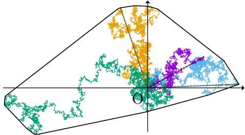
Figure 1: Trajectory of a $2$-d RBM (approximated by 15000 discrete steps) where the dashed lines indicate the resetting to the origin and the colors distinguish the trajectories between the resets for clarity. The black polygon represents the convex hull of the trajectory.

In this paper, our main goal is to investigate how these results (5) and (6) get modified when the resetting rate $r>0$ is switched on, in other words we want to compute the mean perimeter and the mean area of the $2$-d RBM. Since the position distribution of the $2$-d RBM reaches a stationary state at long times, one would have perhaps naively guessed that both $\langle L(t)\rangle$ and $\langle A(t)\rangle$ would become time-independent at late times. Our exact computations show that this naive guess is not correct. The mean perimeter increases very slowly as $\langle L(t)\rangle\propto\ln(rt)$ at long times $t\gg 1/r$, while the mean area increases as $\langle A(t)\rangle\propto\ln^{2}(rt)$, for $t\gg 1/r$. Actually, in this paper we compute both $\langle L(t)\rangle$ and $\langle A(t)\rangle$ exactly for all $t$. Our results can be summarised as follows. We get, for all $t$,

$$\langle L(t)\rangle=2\pi\sqrt{\frac{D}{r}}\,f_{1}(rt)$$ (7)

$$\langle A(t)\rangle=2\pi\,{\frac{D}{r}}\,f_{2}(rt)$$ (8)

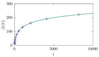
(a)

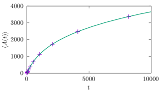
(b)

Figure 5: The mean 4(a) perimeter $\langle L(t)\rangle$ and 4(b) area $\langle A(t)\rangle$ plotted as a function of time $t$. The solid lines represent the exact result 4(a) $\langle L(t)\rangle=2\,\pi\,\sqrt{\frac{D}{r}}\,f_{1}(r\,t)$ given in Eq. (61) and 4(b) $\langle A(t)\rangle=(2D/r)\,f_{2}(rt)$ with $f_{2}(z)$ given in Eq. (65). The symbols represent the respective results from numerical simulations with errorbars smaller than the lines. Here $D=1/2$ and $r=10^{-2}$.

where the scaling functions $f_{1}(z)$ and $f_{2}(z)$ are given explicitly in Eqs. (35) and (65) respectively. Numerical simulations shown in Fig. 5 shows an excellent agreement with our analytical predictions.

The rest of the paper is organised as follows. In Section II we outline the main method, adapting Cauchy’s formula for closed convex curves in two-dimensions, to compute the mean perimeter and the mean area of the $2$-d RBM. In Section III, we compute the first two moments of the expected maximum up to time $t$ of the $x$-component of the $2$-d RBM. In Section IV, we compute the mean square displacement of the $y$-component at the time at which the $x$-component reaches is maximum over the interval $[0,t]$. We then use the exact results from Sections III and IV to finally compute the mean perimeter and the mean area of the convex hull of $2$-d RBM in Section V. Finally, we conclude in Section VI. Some details about a Laplace inversion are discussed in Appendix A.

II Mean perimeter and mean area of the convex hull of a $2$-d stochastic process via Cauchy’s formula

Let us briefly recall the key idea developed in Refs. ch1 ; ch2 to compute the mean perimeter and the mean area of the convex hull of an arbitrary $2$-d stochastic process by adapting Cauchy’s formula to a random curve. This procedure is very general and it essentially maps the problem of computing the mean perimeter and the mean area of the convex hull of an arbitrary $2$-d process to the problem of computing the extreme statistics of the one-dimensional component processes in the $x$ and $y$ directions.

Suppose we have an arbitrary convex domain ${\cal D}$ in two dimensions with its boundary ${\cal C}$ parametrized as $\{{\cal X}(s),{\cal Y}(s)\}$, where $s$ denotes the arc distance along the boundary contour ${\cal C}$. According to Cauchy’s formula Cauchy , the perimeter of the convex domain ${\cal D}$ is given by

$$L=\int_{0}^{2\pi}m(\theta)\,d\theta\,,$$ (9)

where $m(\theta)$ is known as the support function defined as

$$m(\theta)=\max\limits_{s}\left[{\cal X}(s)\cos(\theta)+{\cal Y}(s)\sin(\theta)\right]\,.$$ (10)

The quantity $m(\theta)$ has the simple interpretation: it is the maximum of the projections of all points of the boundary curve ${\cal C}$ along the direction $\theta$.

Let us now consider an arbitrary set of $n$ vertices $\{(X_{i},Y_{i}),\,i=1,2,\ldots,n\}$ in $2$-d (e.g., they may represent the positions of a stochastic process in $2$-d at successive times in a given realization) and construct the convex hull ${\cal C}$ of these vertices. The perimeter of the convex hull is given by Cauchy’s formula in Eq. (9). To apply this formula, we need to first evaluate $\{{\cal X}(s),{\cal Y}(s)\}$ of the convex hull ${\cal C}$ and then compute its maximum over $s$. This is clearly a difficult problem. The key observation of Refs. ch1 ; ch2 that bypasses this step is that the support function $m(\theta)$ of the convex hull can be obtained directly from the underlying vertices (without the need to first compute $\{{\cal X}(s),{\cal Y}(s)\}$ of ${\cal C}$ and then maximizing over $s$) as

$$m(\theta)=\max\limits_{1\leq i\leq n}\left[X_{i}\,\cos(\theta)+Y_{i}\,\sin(\theta)\right]\,.$$ (11)

Next Eq. (9) is averaged over all realizations of the stochastic process, i.e., over different realizations of the vertices $\{(X_{i},Y_{i})\}$ to get

$$\langle L_{n}\rangle=\int_{0}^{2\pi}\langle m(\theta)\rangle\,d\theta\,.$$ (12)

Moreover, if the $2$-d process is isotropic (e.g. the RBM process in $2$-d is isotropic), $\langle m(\theta)\rangle$ is independent of $\theta$. Consequently, we can just consider the direction $\theta=0$. This leads to a simplification of Cauchy’s formula as we just need to compute the expected maximum of the one-dimensional component process ch1 ; ch2

$$\langle L_{n}\rangle=2\,\pi\,\langle M_{n}\rangle\,\quad{\rm where}\quad M_{n}=\max\,\left[X_{1},X_{2},\ldots,X_{n}\right]\,.$$ (13)

A similar procedure works for the mean area of the convex hull. It has been shown that the mean area for an arbitrary isotropic $2$-d stochastic process is given by the formula ch1 ; ch2

$$\langle A_{n}\rangle=\pi\left[\langle M_{n}^{2}\rangle-\langle y_{m}^{2}\rangle(n)\right]\;.$$ (14)

Here, $\langle M_{n}^{2}\rangle$ is the second moment of the maximum $M_{n}$ of the one-dimensional $x$ component process as defined in Eq. (13). In Eq. (14) the second term refers to the mean square displacement of the $y$ component at the time when the $x$ component reaches its maximum.

The results (13) and (14) hold for any arbitrary $2$-d isotropic stochastic process in discrete time, with $n$ vertices. For a continuous time $2$-d stochastic process, the analogous formulae read

$$\langle L(t)\rangle=2\,\pi\,\langle M(t)\rangle\;,$$ (15)

$$\langle A(t)\rangle=\pi\left[\langle M^{2}(t)\rangle-\langle y_{m}^{2}\rangle(t)\right]\;,$$ (16)

where $t$ denotes the total duration of the process and

$$M(t)=\max[\{x(\tau)\},\,\forall\,0\leq\tau\leq t]\,.$$ (17)

Here $x(\tau)$ denotes the continuous time $x$-component process. Similarly, $\langle y_{m}^{2}\rangle(t)$ denotes the mean square displacement of the continuous time $y$-component process at the time at which the $x$-component $x(\tau)$ reaches its maximum.

This general procedure has been successfully used in recent years to compute the mean perimeter and the mean area for several $2$-d stochastic processes. These include a single/multiple planar Brownian motions ch1 ; ch2 , planar random acceleration process RMS2011 , $2$-d branching Brownian motion with absorption in the context of epidemic outbreak DMRZ2013 , anomalous diffusion processes in $2$-d LGE2013 , a $2$-d Brownian motion confined in the half-plane CBM12015 ; CBM22015 , discrete-time $2$-d random walks, Lévy flights GLM17 and the run and tumble process in two-dimensions HMSS_2020 . In this paper, we use these formulae in (15) and (16) to compute exactly the mean perimeter and the mean area of the convex hull of the $2$-d RBM.

III The statistics of the maximum of the $1$-d Brownian motion with resetting

Consider the $2$-d RBM with a constant resetting rate $r$. The process starts at the origin in the $2$-d plane at time $\tau=0$. Let $x(\tau)$ denote the $x$ component of this $2$-d reset Brownian motion. Since for a $2$-d RBM, the $x$ and the $y$ components evolve independently between resets, the process $x(\tau)$ just represents a one dimensional Brownian motion, starting at $x(0)=0$, with resetting to the $x=0$ at rate $r$. In this section, we compute the statistics of the maximum $M(t)$ of this one dimensional RBM process $x(\tau)$ up to time $t$. As explained earlier, the first two moments $\langle M(t)\rangle$ and $\langle M^{2}(t)\rangle$ are needed as inputs in the computation of the mean perimeter and the mean area of the convex hull of the $2$-d RBM. In fact, the distribution of the maximum $M(t)$ for a one dimensional RBM was already studied in Ref. EM2011.1 in a slightly different language and context. Here we revisit this problem and present a full derivation of the first two moments explicitly which are needed for our purpose to compute the statistics of the convex hull of the $2$-d problem.

Let $M(t)$ denote the maximum of the process $x(\tau)$, starting at $x(0)=0$, up to time $t$

$$M(t)=\max[\{x(\tau)\},\,\forall\,0\leq\tau\leq t]\,.$$ (18)

Clearly $M(t)\geq 0$ since the process starts at the origin. To compute the statistics of $M(t)$, it is convenient to consider the cumulative distribution of $M(t)$

$$Q_{r}(M,t)={\rm Prob.}[M(t)\leq M]\,,$$ (19)

where the subscript $r$ refers to the process with resetting rate $r$. Let us first define a more general quantity (that will be useful in the next section also) $S_{r}(x_{0},t|M)$ which denotes the probability that the process $x(\tau)$, starting at $x_{0}$, stays below the level $M$ up to time $t$. Thus, this is just the survival probability of the reset Brownian process starting at $x_{0}$, with an absorbing boundary at $x=M$ with $M\geq x_{0}$ (see Fig. 2 for a typical trajectory) EVS_review . If we know the survival probability $S_{r}(x_{0},t|M)$ for all $x_{0}$, the cumulative distribution of the maximum can be simply obtained by setting $x_{0}=0$,

$$Q_{r}(M,t)=S_{r}(0,t|M)\,.$$ (20)

To compute the survival probability $S_{r}(x_{0},t|M)$ we use a simple renewal argument Reset_review that expresses the survival probability of the reset process in terms of the survival probability $S_{0}(x_{0},t|M)$ of the process without reset. Indeed, there are two possibilities: no resetting or at least one resetting in the interval $[0,t]$. If there is no resetting, the survival probability is simply $e^{-rt}\,S_{0}(x_{0},t|M)$. In the latter case, let $t_{1}$ denotes the time at which the first resetting occurs. Then the process renews at $t_{1}$, starting from the origin. Adding up the two contributions we get

$$S_{r}(x_{0},t|M)=e^{-rt}\,S_{0}(x_{0},t|M)+r\,\int_{0}^{t}dt_{1}\,e^{-rt_{1}}\,S_{0}(x_{0},t_{1}|M)\,S_{r}(0,t-t_{1}|M)$$ (21)

The first term corresponds to survival of the process with no resetting in the interval $[0,t]$. In the second term, $re^{-rt_{1}}$ denotes the probability that the first resetting occurs at $t_{1}$. The factor $S_{0}(x_{0},t_{1}|M)$ is the survival probability during this interval $[0,t_{1}]$, while $S_{r}(0,t-t_{1}|M)$ denotes the survival probability during the time interval $[t_{1},t]$. Note that in the second interval, the subscript $r$ shows that the process is with resetting. It is convenient to take the Laplace transform of Eq. (21) so that the convolution structure in the second term on the right hand side (rhs) can be exploited. Defining

$${\tilde{S}}_{r}(x_{0},s|M)=\int_{0}^{\infty}S_{r}(x_{0},t|M)\,e^{-st}\,dt\,,$$ (22)

we get from Eq. (21)

$${\tilde{S}}_{r}(x_{0},s|M)={\tilde{S}}_{0}(x_{0},r+s|M)+r\,{\tilde{S}}_{0}(x_{0},r+s|M)\,{\tilde{S}}_{r}(0,s|M)\,.$$ (23)

Setting $x_{0}=0$, we obtain

$${\tilde{S}}_{r}(0,s|M)=\frac{{\tilde{S}}_{0}(0,r+s|M)}{1-r\,{\tilde{S}}_{0}(0,r+s|M)}\,.$$ (24)

Hence, from Eq. (23)

$${\tilde{S}}_{r}(x_{0},s|M)=\frac{{\tilde{S}}_{0}(x_{0},r+s|M)}{1-r\,{\tilde{S}}_{0}(0,r+s|M)}\,.$$ (25)

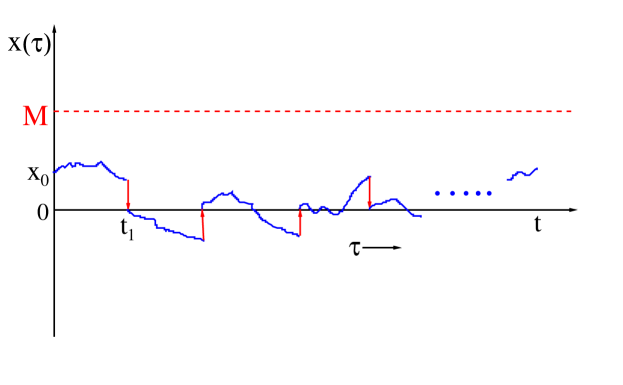
Figure 2: A typical trajectory (schematic) of a $1$-d Brownian motion $x(\tau)$ vs. $\tau$, with resetting to $x=0$ at a constant rate $r$. The process starts at $x(0)=x_{0}$, stays below the level $M$ (with $M\geq x_{0}$ as shown by the dashed (red) line) up to time $t$. The resetting events to the origin are shown by directed (red) arrows, with the first resetting at time $t_{1}$.

The survival probability $S_{0}(x_{0},t|M)$ of an ordinary Brownian motion (with diffusion constant $D$) starting at $x_{0}$ and with an absorbing boundary at $M$ can be very easily computed using the method of images Redner_Book . Equivalently, its Laplace transform can be computed directly by solving a backward Fokker-Planck equation BF_2005 ; Persistence_review . Indeed, $S_{0}(x_{0},t|M)$ satisfies the backward Fokker-Planck equation

$$\frac{\partial S_{0}}{\partial t}=D\,\frac{\partial^{2}S_{0}}{\partial x_{0}^{2}}$$ (26)

in the region $x_{0}\in[-\infty,M]$ with absorbing boundary condition at $x_{0}=M$, i.e, $S_{0}(x_{0}=M,t|M)=0$ and $S_{0}(x_{0}\to-\infty,t|M)=1$ for all $t$. The last condition follows from the fact that if the particle starts at $-\infty$, it definitely stays below $M$ for any finite $t$. The initial condition is $S_{0}(x_{0},0|M)=1$ for all $x_{0}<M$. Taking the Laplace transform of Eq. (26) with respect to $t$ and using the initial condition gives

$$-1+s\,{\tilde{S}}_{0}(x_{0},s|M)=D\,\frac{d^{2}{\tilde{S}}_{0}}{dx_{0}^{2}}\,.$$ (27)

The solution, using the two boundary conditions, reads for $x_{0}\leq M$

$${\tilde{S}}_{0}(x_{0},s|M)=\frac{1}{s}\,\left[1-e^{-\sqrt{\frac{s}{D}}\,(M-x_{0})}\right]\,.$$ (28)

This Laplace transform can be explicitly inverted to give

$$S_{0}(x_{0},t|M)={\rm erf}\left(\frac{M-x_{0}}{\sqrt{4Dt}}\right)\,;\quad\,\,{\rm erf}(z)=\frac{2}{\sqrt{\pi}}\,\int_{0}^{z}e^{-u^{2}}\,du\,,$$ (29)

which coincides, as expected, with the survival probability up to $t$ of an ordinary Brownian motion, starting at $M-x_{0}\geq 0$ and with an absorbing boundary at the origin Redner_Book ; Persistence_review . However, for our purpose, the Laplace transform of this survival probability in Eq. (28) is more useful.

Indeed, substituting the result from Eq. (28) on the rhs of Eq. (25) gives our desired quantity

$${\tilde{S}}_{r}(x_{0},s|M)=\frac{1-e^{-\sqrt{\frac{(r+s)}{D}}\,(M-x_{0})}}{s+r\,e^{-\sqrt{\frac{(r+s)}{D}}\,M}}\,.$$ (30)

Setting $x_{0}=0$ in Eq. (30) and using Eq. (20) we get the Laplace transform of the cumulative distribution of the maximum (for the process starting at the origin)

$${\tilde{Q}}_{r}(M,s)=\int_{0}^{\infty}Q_{r}(M,t)\,e^{-st}\,dt=\frac{1-e^{-\sqrt{\frac{(r+s)}{D}}\,M}}{s+re^{-\sqrt{\frac{(r+s)}{D}}\,M}}\,.$$ (31)

The probability density function (PDF) $P_{r}(M,t)$ of the maximum $M(t)$ can be obtained from the cumulative distribution by just taking a derivative, $P_{r}(M,t)=\partial_{M}Q_{r}(M.t)$. Hence, its Laplace transform, obtained by taking derivative of Eq. (31), reads

$${\tilde{P}}_{r}(M,s)=\int_{0}^{\infty}P_{r}(M,t)\,e^{-st}\,dt=\frac{(r+s)^{3/2}}{\sqrt{D}}\,\frac{e^{-\sqrt{\frac{(r+s)}{D}}\,M}}{\left(s+r\,e^{-\sqrt{\frac{(r+s)}{D}}\,M}\right)^{2}}\,.$$ (32)

It is difficult to invert this Laplace transform explicitly, except at late times EM2011.1 when the PDF $P_{r}(M,t)$ can be shown to converge to the Gumbel law EM2011.1 . For our purpose, namely to compute the mean perimeter and the mean area of the convex hull of the $2$-d RBM, we only need the first two moments. The first moment $\langle M(t)\rangle$ was already computed explicitly for all $t$ EM2011.1 which we reproduce below for the sake of completeness. Here we show that the second moment $\langle M^{2}(t)\rangle$ can also be computed explicitly for all $t$.

III.1 Expected maximum $\langle M(t)\rangle$

The Laplace transform of the expected maximum is given by

$$\int_{0}^{\infty}\langle M(t)\rangle\,e^{-st}\,dt=\int_{0}^{\infty}M\,{\tilde{P}}_{r}(M,s)\,dM\,.$$ (33)

Using the explicit result in Eq. (32) and performing the integral gives

$$\int_{0}^{\infty}\langle M(t)\rangle\,e^{-st}\,dt=\frac{\sqrt{D\,(r+s)}}{r\,s}\,\ln\left(\frac{r+s}{s}\right)\,.$$ (34)

Fortunately, this Laplace transform can be explicitly inverted EM2011.1 and we present its derivation in Appendix A. This gives

$$\langle M(t)\rangle=\sqrt{\frac{D}{r}}\,f_{1}(r\,t)\,;\quad{\rm where}\quad f_{1}(z)=\int_{0}^{z}\frac{dy}{y}\,(1-e^{-y})\,\left[\frac{e^{-(z-y)}}{\sqrt{\pi\,(z-y)}}+{\rm erf}\left(\sqrt{z-y}\right)\right]\,,$$ (35)

where ${\rm erf}(z)=(2/\sqrt{\pi})\,\int_{0}^{z}e^{-u^{2}}\,du$ is the error function. The asymptotic behaviors of the scaling function $f_{1}(z)$, for small and large $z$, can be easily derived. One gets to leading orders EM2011.1

$$f_{1}(z)\approx\begin{cases}\frac{2}{\sqrt{\pi}}\,\sqrt{z}{-\frac{1}{45\sqrt{\pi}}z^{5/2}}\quad\,{\rm as}\quad z\to 0\\ \\ \ln z+\gamma_{E}\quad\;\;\;\hskip 31.2982pt{\rm as}\quad z\to\infty\;,\end{cases}$$ (36)

where $\gamma_{E}=0.57721\ldots$ is the Euler constant.

The asymptotic behaviors of $\langle M(t)\rangle$ for $t\ll 1/r$ and $t\gg 1/r$ then follow readily. One gets EM2011.1

$$\langle M(t)\rangle\approx\begin{cases}\sqrt{Dt}\left[\sqrt{\frac{4}{\pi}}{-\frac{1}{45\sqrt{\pi}}(rt)^{2}}\right]\,\quad\quad\quad{\rm for}\quad t\ll\frac{1}{r}\\ \\ \sqrt{\frac{D}{r}}\,\left[\ln(rt)+\gamma_{E}\right]\quad\hskip 45.52458pt{\rm for}\quad t\gg\frac{1}{r}\;.\end{cases}$$ (37)

The leading term in the first line can be simply understood as follows. Since $1/r$ is the typical time for a resetting even to take place, when $t\ll 1/r$ the particle has hardly undergone any resetting and hence it behaves as a free Brownian motion. Indeed, the leading term in the first line of Eq. (37) corresponds exactly to the expected maxima of an ordinary Brownian motion EVS_review . The result for large $t\gg 1/r$ is more interesting. As was shown in Refs. EM2011.1 ; MSS2015 , the RBM approaches a stationary state when $t\gg 1/r$ due to the repeated resettings. Nevertheless, the expected maximum up to time $t$ still increases with time, albeit very slowly as a logarithm. This can be understood heuristically using the theory of extreme value statistics (EVS) of weakly correlated variables EM2011.1 ; Reset_review ; EVS_review . The scaling function $f_{1}(z)$ describes the full crossover from the early time Brownian growth of the expected maximum to the late time logarithmic growth.

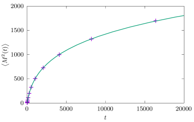
Figure 3: The second moment $\langle M^{2}(t)\rangle$ plotted as a function of time $t$. The solid line represents the exact result $\langle M^{2}(t)\rangle=(2D/r)\,H(rt)$ with $H(z)$ given in Eq. (41), while the symbols represent the results from numerical simulations. Here $D=1/2$ and $r=10^{-2}$.

III.2 The second moment $\langle M^{2}(t)\rangle$

The Laplace transform of the second moment is given by

$$\int_{0}^{\infty}\langle M^{2}(t)\rangle\,e^{-st}\,dt=\int_{0}^{\infty}M^{2}\,{\tilde{P}}_{r}(M,s)\,dM\,.$$ (38)

Using the result for ${\tilde{P}}_{r}(M,s)$ from Eq. (32) and carrying out integration we get

$$\int_{0}^{\infty}\langle M^{2}(t)\rangle\,e^{-st}\,dt=-\frac{2D}{r\,s}\,{\rm Li}_{2}\left(-\frac{r}{s}\right)\,;\quad{\rm where}\quad{\rm Li}_{2}(z)=\sum_{k=1}^{\infty}\frac{z^{k}}{k^{2}}\,.$$ (39)

Substituting the series expansion of the PolyLog function ${\rm Li}_{2}(-r/s)$ we can then invert the Laplace transform term by term, by using ${\cal L}_{s}^{-1}\left(s^{-(k+1)}\right)=t^{k}/k!$, where ${\cal L}_{s}^{-1}$ denotes the Laplace inverse with respect to $s$. This gives

$$\langle M^{2}(t)\rangle=\frac{2D}{r}\,H(r\,t)$$ (40)

where the scaling function $H(z)$ is given by

$$H(z)=\sum_{n=1}^{\infty}\frac{(-1)^{n+1}}{n^{2}}\,\frac{z^{n}}{n!}=z\,_{3}F_{3}\left[\{1,1,1\},\{2,2,2\};-z\right]\,,$$ (41)

where ${}_{p}F_{q}$ is the generalised hypergeometric series GR . The asymptotic behaviors of the scaling function $H(z)$ are given by

$$H(z)\approx\begin{cases}z-\frac{z^{2}}{8}\quad\,{\rm as}\quad z\to 0\\ \\ \frac{1}{12}\left[6\,\ln^{2}z+12\,\gamma_{E}\,\ln z+6\,\gamma_{E}^{2}+\pi^{2}\right]\quad{\rm as}\quad z\to\infty\end{cases}$$ (42)

This then gives the asymptotic behaviors of $\langle M^{2}(t)\rangle$ from Eq. (39). Once again, for $t\ll 1/r$, one recovers the Brownian result, $\langle M^{2}(t)\rangle\approx 2\,D\,t$ as expected, while for large $t\gg 1/r$, it grows as $\langle M^{2}(t)\rangle\approx(D/r)\,\ln^{2}(rt)$ to leading order. In Fig. 3 we compare our analytical prediction for $\langle M^{2}(t)\rangle$ in Eqs. (39) along with Eq. (41) with numerical simulations, finding excellent agreement for all $t$.

IV Computation of the second moment $\langle y_{m}^{2}\rangle(t)$

In this section, we compute another ingredient needed for the calculation of the mean area of the convex hull. Let $\{x(\tau),y(\tau)\}$ denote the $x$ and the $y$ component process of the $2$-d Brownian motion starting at the origin $\{x(0)=0,y(0)=0\}$ and resetting to the origin. When the resetting occurs, both the $x$ and the $y$ component are reset simultaneously to $x(0)=0$ and $y(0)=0$ respectively. Thus resetting makes the two component processes highly correlated. Let $t_{m}$ denote the time at which the $x$-component achieves its maximum value, say $M$, in the interval $[0,t]$. For the computation of the mean area, we need to compute $\langle y_{m}^{2}\rangle(t)$ where $y_{m}=y(\tau=t_{m})$ denotes the value of the $y$ component exactly at the time $\tau=t_{m}$ when the $x$ component achieves its maximum in the interval $[0,t]$. Let us briefly recall how to compute this for a standard $2$-d Brownian motion in the absence of resetting, i.e., when the reset rate $r=0$ ch1 ; ch2 . In this case, since there is no correlation between the $x$ and the $y$ component with each of them performing independent Brownian motion, it follows that $\langle y^{2}(\tau)\rangle=2\,D\,\tau$ for any $\tau$. Hence, in this case $\langle y_{m}^{2}\rangle(t)=2\,D\,\langle t_{m}\rangle=D\,t$ where one uses $\langle t_{m}\rangle=t/2$ for the $x$ component which is just a one dimensional free Brownian motion. However, this simple argument does not work in the presence of a finite resetting rate $r>0$ since the two components get strongly correlated via the resetting events. Nevertheless, $\langle y_{m}^{2}\rangle(t)$ can be computed explicitly for all $t$ as we show in this section.

Before starting the computation for $\langle y_{m}^{2}\rangle(t)$ for the Brownian motion with resetting, let us first briefly recall some basic facts about the Brownian motion in the absence of resetting ($r=0$). Consider first the Green’s function or the propagator for a $2$-d Brownian motion. This is just the probability density $G_{0}(x,y;\tau)$ that the Brownian motion, starting at the origin $(0,0)$ reaches $(x,y)$ at time $\tau$ and is simply given by the product of two one dimensional propagators

$$G_{0}(x,y,\tau)=\frac{1}{4\,\pi\,D\,\tau}\,e^{-\frac{x^{2}+y^{2}}{4\,D\,\tau}}\,.$$ (43)

If however one puts an absorbing boundary at $x=M$, then the constrained propagator of the same process to reach $(x\leq M,y)$ at time $\tau$, while staying below the level $M$ during the whole interval $[0,\tau]$, can be easily obtained using the method of images Redner_Book ; BF_2005 . One gets

$$G_{0}(x,y,\tau|M)=\frac{1}{4\,\pi\,D\,\tau}\,e^{-\frac{y^{2}}{4\,D\,\tau}}\,\left[e^{-\frac{x^{2}}{4\,D\,\tau}}-e^{-\frac{(2M-x)^{2}}{4\,D\,\tau}}\right]\,.$$ (44)

We will need this result shortly.

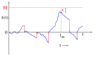
(a)

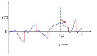
(b)

Figure 4: A typical trajectory for the (a) $x$-component: $x(\tau)$ vs. $\tau$ for $\tau\in[0,t]$ and the (b) $y$ component: $y(\tau)$ vs. $\tau$ over the same interval $\tau\in[0,t]$, both starting at the origin at $\tau=0$. When a reset event happens (shown by (red) arrows), both $x$ and $y$ components are simultaneously reset to $0$. Between resets, they evolve independently. The (red) dashed line indicates the maximum value $M$ of $x(\tau)$ in the interval $[0,t]$ and it arrives at this maximum (actually at $x=M-\epsilon$ where $\epsilon$ is a small cut-off (see text)) at time $t_{m}$. The value of the $y$ component at $\tau=t_{m}$ is denoted by $y(\tau=t_{m})=y_{m}$.

We now switch on the resetting with a constant rate $r$ and our goal is to compute the second moment $\langle y_{m}^{2}\rangle$ of the $y$ component at the time $t_{m}$ at which the $x$ component achieves its maximum within the time interval $[0,t]$. To compute this quantity, we first need to compute the probability of a path of the process satisfying all the constraints. This is done by using a path decomposition procedure that exploits the Markov property of the process, as explained below. This computation is best explained with the help of Fig. 4, where we plot schematically the trajectories of both the $x$ (left) and the $y$ component (right) in the time interval $[0,t]$, both starting at $0$ at $\tau=0$. Let $t_{m}$ denote the time at which $x(\tau)$ achieves its maximum value $M$ in $[0,t]$. This instant $t_{m}$ divides the full interval $[0,t]$ into two halves: the left half during $[0,t_{m}]$ and the right half during $[t_{m},t]$. On the left half, the $x$ component starts at the origin, and has to stay below the level $M$ till $t_{m}$ and arrive at $M$ exactly at $t_{m}$. On the right half, the process stays below the level $M$ during $[t_{m},t]$. This restriction of staying below a given level is usually implemented by putting an absorbing boundary condition at $x=M$. However, putting this absorbing boundary at $x=M$ will forbid the Brownian process to reach $x=M$ at $t_{m}$. To circumvent this difficulty, we can put a small cut-off $\epsilon$ and say that the particle reaches the value $M-\epsilon$ at time $t_{m}$—then there is no problem in employing the absorbing boundary during the full interval $[0,t]$. At the end of the calculation we will take the limit $\epsilon\to 0$ in an appropriate way. While this procedure is perhaps not mathematically fully rigorous, it provides the quickest (and also a physically transparent) way to arrive at the correct final result. This limiting procedure using $\epsilon$ cut-off has been successfully used in several examples of constrained Brownian motions before MC_2005 ; MRKY_2008 ; SL_2010 ; PCMS_2013 ; PCMS_2015 ; MMS_2019 ; MMS_2020 . Below we will use the same procedure for this problem also.

Let us first focus on the first interval $\tau\in[0,t_{m}]$. In this interval, the $x$ component of the reset process, starting at the origin and staying below $M$, reaches the position $M-\epsilon$ exactly at $t_{m}$. The $y$ component, starting at the origin and undergoing resettings at the same times as the $x$ process, reaches $y_{m}$ at $\tau=t_{m}$. Note that the $y$ process is not restricted to be below $M$. We then want to compute the propagator, i.e., the joint probability density $G_{r}(x=M-\epsilon,y=y_{m},\tau=t_{m}|M)$ for the two components to reach respectively $M-\epsilon$ and $y_{m}$, with the former only staying below the level $M$. The subscript $r$ in $G_{r}$ denotes the presence of resetting to the origin with rate $r$. This propagator can again be computed using the renewal method. We can write, as in Eq. (21) in the previous section,

$$G_{r}(M-\epsilon,y_{m},t_{m}|M)=G_{0}(M-\epsilon,y_{m},t_{m}|M)\,e^{-r\,t_{m}}+r\,\int_{0}^{t_{m}}dt_{1}\,e^{-r\,t_{1}}\,S_{0}(0,t_{1}|M)\,G_{r}(M-\epsilon,y_{m},t_{m}-t_{1}|M)\,,$$ (45)

where $S_{0}(0,t_{1}|M)$ denotes the survival probability of the $x$ component, i.e., a one dimensional Brownian reset process up to time $t_{1}$, starting at the origin and with an absorbing boundary at $x=M$. This is exactly the quantity whose Laplace transform we already computed in Eq. (28) in the previous section. The quantity $G_{0}(M-\epsilon,y_{m},t_{m}|M)$ is already computed in Eq. (44). In Eq. (45), the first term represents no resetting while the second term counts the contributions from at least one resetting. For this we consider the first resetting at $t_{1}$ that occurs before $t_{m}$, and after that the process renews. During $[0,t_{1}]$ the $x$ process stays below $M$ which is ensured by the factor $S_{0}(0,t_{1}|M)$ inside the integral on the rhs of Eq. (45). Note that for the $y$ process we have no restriction whatsoever. The factor $G_{r}(M-\epsilon,y_{m},t_{m}-t_{1}|M)$ ensures that the renewed $(x,y)$ process starting at $t_{1}$ from the origin arrives at $(M-\epsilon,y_{m})$ after a time $t_{m}-t_{1}$, with the $x$ component staying below $M$ during $t_{m}-t_{1}$. We take the product and integrate over $t_{1}$ from $0$ to $t_{m}$. Again, the convolution structure of Eq. (45) signals that it simplifies in the Laplace space (with respect to time). Indeed, defining ${\tilde{G}}_{r}(x,y,s|M)=\int_{0}^{\infty}G_{r}(x,y,t_{m}|M)\,e^{-s\,t_{m}}\,dt_{m}$ and taking the Laplace transform of Eq. (45) with respect to $t_{m}$ gives

$${\tilde{G}}_{r}(M-\epsilon,y_{m},s|M)=\frac{{\tilde{G}}_{0}(M-\epsilon,y_{m},r+s|M)}{1-r\,{\tilde{S}}_{0}(0,r+s)|M)}=\frac{(r+s)\,{\tilde{G}}_{0}(M-\epsilon,y_{m},r+s|M)}{s+r\,e^{-\sqrt{\frac{r+s}{D}}\,M}}\,,$$ (46)

where we used the expression for ${\tilde{S}}_{0}(0,r+s)|M)$ from Eq. (28). The relation in Eq. (46) expresses the constrained Green’s function of the process with resetting in terms of the constrained Green’s function without resetting $G_{0}$ computed in Eq. (44).

We now focus on the second time interval $\tau\in[t_{m},t]$. This is easy because during this interval we just have to ensure that only the $x$ process, starting at $M-\epsilon$ at time $t_{m}$, stays below the level $M$ during the interval $[t_{m},t]$. For the $y$ process we have no restriction. Hence this probability is simply $S_{r}(M-\epsilon,t-t_{m}|M)$, i.e., the survival probability for the $x$ process during the interval $[t_{m},t]$, starting at $M-\epsilon$ at time $t_{m}$, with an absorbing boundary at $M$. The Laplace transform of this probability has already been computed in Eq. (30).

The total probability of such a constrained path of the joint $x$ and $y$ processes is then proportional to the product of the probabilities in the first ($[0,t_{m}]$) and the second ($[t_{m},t]$) time intervals–this follows from the Markov property of the process. We denote this total probability by $P_{r}(M,t_{m},y_{m}|t,\epsilon)$ where $M$, $t_{m}$ and $y_{m}$ are random variables, while $t$ and $\epsilon$ are fixed parameters. Taking this product gives

$$P_{r}(M,t_{m},y_{m}|t,\epsilon)={\cal N}(\epsilon)\,G_{r}(M-\epsilon,y_{m},t_{m}|M)\,S_{r}(M-\epsilon,t-t_{m}|M)\,,$$ (47)

where ${\cal N}(\epsilon)$ is just a normalization constant, such that the joint probability density $P_{r}(M,t_{m},y_{m}|t,\epsilon)$ is normalized to unity when integrated over $M$, $t_{m}$ and $y_{m}$. In principle, ${\cal N}(\epsilon)$ can also depend on $t$. However here, we assume and verify a posteriori that it is indeed independent of $t$.

Let us first integrate over $t_{m}$. This gives the joint probability density of $M$ and $y_{m}$

$$P_{r}(M,y_{m}|t,\epsilon)={\cal N}(\epsilon)\,\int_{0}^{t}G_{r}(M-\epsilon,y_{m},t_{m}|M)\,S_{r}(M-\epsilon,t-t_{m}|M)\,dt_{m}\,.$$ (48)

It is convenient to take the Laplace transform of Eq. (48) with respect to $t$ to get

$${\tilde{P}}_{r}(M,y_{m}|s,\epsilon)=\int_{0}^{\infty}P_{r}(M,y_{m}|t,\epsilon)\,e^{-s\,t}\,dt={\cal N}(\epsilon)\,{\tilde{G}}_{r}(M-\epsilon,y_{m},s|M)\,{\tilde{S}}_{r}(M-\epsilon,s|M)\,.$$ (49)

We now use the explicit expressions for ${\tilde{G}}_{r}(M-\epsilon,y_{m},s|M)$ from Eq. (46) and ${\tilde{S}}_{r}(M-\epsilon,s|M)$ from Eq. (30) to get

$${\tilde{P}}_{r}(M,y_{m}|s,\epsilon)={\cal N}(\epsilon)\,\frac{(r+s)\,\left(1-e^{-\sqrt{\frac{r+s}{D}}\,\epsilon}\right)}{\left(s+r\,e^{-\sqrt{\frac{r+s}{D}}\,M}\right)^{2}}\,{\tilde{G}}_{0}(M-\epsilon,y_{m},r+s|M)\,.$$ (50)

Using the expression for $G_{0}$ from Eq. (44) we then obtain

$${\tilde{P}}_{r}(M,y_{m}|s,\epsilon)={\cal N}(\epsilon)\,\frac{(r+s)\,\left(1-e^{-\sqrt{\frac{r+s}{D}}\,\epsilon}\right)}{\left(s+r\,e^{-\sqrt{\frac{r+s}{D}}\,M}\right)^{2}}\,\int_{0}^{\infty}\frac{dT}{4\,\pi\,D\,T}\,e^{-(r+s)\,T}\,e^{-\frac{y_{m}^{2}}{4\,D\,T}}\,\left[e^{-\frac{(M-\epsilon)^{2}}{4\,D\,T}}-e^{-\frac{(M+\epsilon)^{2}}{4\,D\,T}}\right]\,.$$ (51)

We now take the $\epsilon\to 0$ limit. To leading order in $\epsilon$ it gives

$${\tilde{P}}_{r}(M,y_{m}|s,\epsilon\to 0)=\left[\lim_{\epsilon\to 0}{\cal N}(\epsilon)\,\epsilon^{2}\right]\,\frac{(r+s)^{3/2}}{D^{3/2}\,\left(s+r\,e^{-\sqrt{\frac{r+s}{D}}\,M}\right)^{2}}\,\int_{0}^{\infty}\frac{dT}{4\,\pi\,D\,T}\,e^{-(r+s)\,T}\,e^{-\frac{y_{m}^{2}}{4\,D\,T}}\,\frac{M}{T}\,e^{-\frac{M^{2}}{4\,D\,T}}\,.$$ (52)

To determine the normalization constant, we integrate Eq. (52) over $y_{m}$ to get the Laplace transform of the marginal distribution of $M$

$${\tilde{P}}_{r}(M,s)=\int_{-\infty}^{\infty}{\tilde{P}}_{r}(M,y_{m}|s,\epsilon\to 0)\,dy_{m} = \left[\lim_{\epsilon\to 0}{\cal N}(\epsilon)\,\epsilon^{2}\right]\,\frac{(r+s)^{3/2}}{D^{3/2}\,\left(s+r\,e^{-\sqrt{\frac{r+s}{D}}\,M}\right)^{2}}\,\frac{M}{\sqrt{4\,\pi\,D}}\,\int_{0}^{\infty}\frac{dT}{T^{3/2}}\,e^{-(r+s)\,T-\frac{M^{2}}{4\,D\,T}}\,$$ (53)

$$= \left[\lim_{\epsilon\to 0}{\cal N}(\epsilon)\,\epsilon^{2}\right]\,\frac{(r+s)^{3/2}}{D^{3/2}\,\left(s+r\,e^{-\sqrt{\frac{r+s}{D}}\,M}\right)^{2}}\,e^{-\sqrt{\frac{r+s}{D}}\,M}\,,$$

where the integral over $T$ is performed explicitly using the identity $\int_{0}^{\infty}dT\,T^{-3/2}\,e^{-aT-b/T}=\sqrt{\frac{\pi}{b}}\,e^{-2\,\sqrt{a\,b}}$ for $a$ and $b$ positive. However, ${\tilde{P}}_{r}(M,s)$ was already computed in Eq. (32). Hence, comparing the rhs of Eqs. (53) and (32) we immediately get the normalization constant

$$\lim_{\epsilon\to 0}{\cal N}(\epsilon)\,\epsilon^{2}=D\,.$$ (54)

Using this normalization constant in Eq. (52) finally gives the Laplace transform of the joint distribution of $M$ and $y_{m}$

$${\tilde{P}}_{r}(M,y_{m},s)={\tilde{P}}_{r}(M,y_{m}|s,\epsilon\to 0)=\frac{M\,(r+s)^{3/2}}{{D}^{3/2}\,\left(s+r\,e^{-\sqrt{\frac{r+s}{D}}\,M}\right)^{2}}\,\int_{0}^{\infty}\frac{dT}{4\,\pi\,T^{2}}\,e^{-(r+s)\,T-\frac{(M^{2}+y_{m}^{2})}{4\,D\,T}}\,.$$ (55)

From this joint distribution, we can then compute the Laplace transform of $\langle y_{m}^{2}\rangle(t)$ as

$$\int_{0}^{\infty}\langle y_{m}^{2}\rangle(t)\,e^{-s\,t}\,dt=\int_{0}^{\infty}dM\,\int_{-\infty}^{\infty}dy_{m}\,y_{m}^{2}\,{\tilde{P}}_{r}(M,y_{m},s)\,.$$ (56)

Substituting Eq. (55) on the rhs of Eq. (56) and carrying out the integrals over $y_{m}$ and $T$ explicitly we finally get a relatively simple expression

$$\int_{0}^{\infty}\langle y_{m}^{2}\rangle(t)\,e^{-s\,t}\,dt=D\,\int_{0}^{\infty}dm\,\frac{m\,e^{-m}}{\left(s+r\,e^{-m}\right)^{2}}\,,$$ (57)

where we made a change of variable $m=\sqrt{(r+s)/D}\,M$ in the integral over $M$. We can now invert the Laplace transform in Eq. (57) using ${\cal L}_{s}^{-1}\left[(s+a)^{-2}\right]=t\,e^{-a\,t}$. This gives our final result in this section

$$\langle y_{m}^{2}\rangle(t)=D\,t\,\int_{0}^{\infty}dm\,m\,e^{-m-r\,t\,e^{-m}}=\frac{2\,D}{r}\,V(r\,t)\,$$ (58)

with the scaling function $V(z)$ given by

$$V(z)=\frac{z}{2}\,\int_{0}^{\infty}dm\,m\,e^{-m-z\,e^{-m}}=\frac{1}{2}\,(\Gamma[0,z]+\ln z+\gamma_{E})\,,$$ (59)

where $\Gamma[0,z]=\int_{z}^{\infty}\frac{e^{-t}}{t}\,dt$. It has the asymptotics behaviors

$$V(z)\approx\begin{cases}\frac{z}{2}-\frac{z^{2}}{8}+O(z^{3})\quad\quad\quad\quad\,{\rm as}\quad z\to 0\;,\\ \\ \frac{1}{2}\,(\ln z+\gamma_{E})+O(1/z)\quad\,{\rm as}\quad z\to\infty\;.\end{cases}$$ (60)

V The mean perimeter and the mean area of the convex hull

With all the basic ingredients derived in the previous two sections, we then go on to compute the mean perimeter and the mean area of the convex hull of the $2$-d Brownian motion with resetting to the origin. As discussed in Section-II, the mean perimeter of the convex hull of an isotropic $2$-d stochastic process is given by $\langle L(t)\rangle=2\,\pi\,\langle M(t)\rangle$, where $\langle M(t)\rangle$ is the expected maximum of the one dimensional $x$ component process up to time $t$. Using the result from Eq. (35) we then obtain the exact result for the mean perimeter of the convex hull of the $2$-d RBM for all $t$

$$\langle L(t)\rangle=2\,\pi\,\sqrt{\frac{D}{r}}\,f_{1}(r\,t)$$ (61)

where the scaling function $f_{1}(z)$ is given in Eq. (35) with asymptotic behaviors in Eq. (36). Using the asymptotic behavior of $f_{1}(z)$ in the limit $z\to 0$, we find that for $t\ll 1/r$, $\langle L(t)\approx\sqrt{16\pi Dt}\rangle$, thus recovering the Brownian result in Eq. (5), as expected. In contrast, for $t\gg 1/r$, the mean perimeter grows logarithmically

$$\langle L(t)\rangle\approx 2\,\pi\,\sqrt{\frac{D}{r}}\,\ln(rt)\,.$$ (62)

Our numerical simulations show perfect agreement with our analytical prediction for all $t$ (see Fig. 54(a)).

The mean area of the convex hull is given by (see Section-II)

$$\langle A(t)\rangle=\pi\,\left[\langle M^{2}(t)\rangle-\langle y_{m}^{2}\rangle(t)\right]\,.$$ (63)

Using the explicit results for $\langle M^{2}(t)\rangle$ from Eq. (40) and for $\langle y_{m}^{2}\rangle(t)$ from Eq. (58) we get, for all $t$,

$$\langle A(t)\rangle=\frac{2\pi D}{r}\,f_{2}(rt)\,,$$ (64)

where the scaling function $f_{2}(z)$ is given by

$$f_{2}(z)=H(z)-V(z)=z\,\,_{3}F_{3}\left[\{1,1,1\},\{2,2,2\},-z\right]-\frac{1}{2}\left[\Gamma[0,z]+\ln z+\gamma_{E}\right]\,.$$ (65)

It has the following asymptotic behaviors

$$f_{2}(z)\approx\begin{cases}&\frac{z}{2}-\frac{z^{3}}{108}++\frac{z^{4}}{384}\quad\,{\rm as}\quad z\to 0\\ \\ &\frac{1}{2}\left[\ln^{2}z+\left(2\gamma_{E}-1\right)\,\ln z+\gamma_{E}^{2}-\gamma_{E}+\frac{\pi^{2}}{6}\right]+O(1/z)\quad{\rm as}\quad z\to\infty\end{cases}$$ (66)

Note that when $t\ll 1/r$, using $f_{2}(z)\approx z/2$ as $z\to 0$, we recover the standard Brownian motion result $\langle A(t)\rangle\approx\pi\,D\,t$ in Eq. (6). In contrast, for large $t\gg 1/r$, the mean area of the convex hull grows as

$$\langle A(t)\rangle\approx\pi\,\frac{D}{r}\,\ln^{2}(rt)\,.$$ (67)

In Fig. 54(b), we compare our analytical prediction with numerical simulations, finding excellent agreement for all $t$.

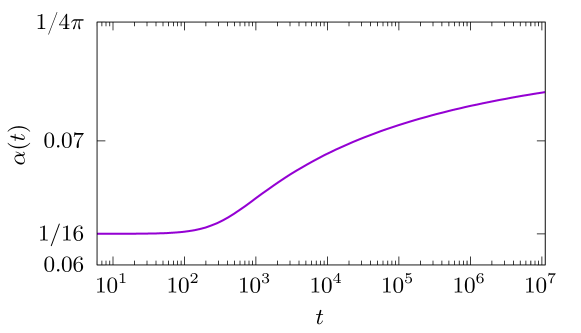
Figure 6: Plot of $\alpha(t)={\langle A(t)\rangle}/{[\langle L(t)\rangle]^{2}}$, given in Eq. (69) together with Eqs. (35) and (65), as a function of $t$, on a log-log scale, for $D=1/2$ and $r=10^{-2}$. When $t\to\infty$, $\alpha(t)\to 1/(4\pi)$, which shows that the convex hull reaches a circular shape. Note however that this convergence to a circular shape is quite slow [from Eq. (70), one sees that $1/(4\pi)-\alpha(t)\propto 1/(\ln(rt))$, as $t\to\infty$].

Let us point out an interesting geometric fact that emerged from our exact results. For a perfect circle of radius $R$, the perimeter is $L=2\pi R$ while the area is $A=\pi R^{2}$. Hence the dimensionless ratio

$$\alpha=\frac{A}{L^{2}}=\frac{1}{4\pi}\,.$$ (68)

The isoperimetric inequality says that for any arbitrary shape in two dimensions $\alpha\leq 1/(4\pi)$, i.e, the isoperimetric upper bound is saturated by the circular shape. The closer the value of $\alpha$ to this upper bound $1/(4\pi)$, the more circular is the shape of the domain. Now, for the convex hull of a planar RBM, our exact results in Eqs. (61) and (64) show that the ratio

$$\alpha(t)=\frac{\langle A(t)\rangle}{[\langle L(t)\rangle]^{2}}=F(rt)\,;\quad\,\,{\rm where}\quad\,F(z)=\frac{1}{2\pi}\,\frac{f_{2}(z)}{f_{1}^{2}(z)}\,$$ (69)

valid at any time $t$, with the scaling functions $f_{1}(z)$ and $f_{2}(z)$ given respectively in Eqs. (35) and (65). The function $F(z)$ has the asymptotic behaviors

$$F(z)\approx\begin{cases}&\frac{1}{16}\left(1+\frac{1}{270}z^{2}\right)\quad\,{\rm as}\quad z\to 0\\ \\ &\frac{1}{4\pi}\left(1-\frac{1}{\ln z}\right)\quad\quad{\rm as}\quad z\to\infty\;.\end{cases}$$ (70)

Hence, for $t\ll 1/r$, when the RBM effectively behaves like a Brownian motion without resetting, the ratio $\alpha(t)\approx 1/16<1/(4\pi)$, indicating that at short times the shape of the convex hull is far from circular. In contrast, for $t\gg 1/r$, $\alpha(t)\approx 1/(4\pi)$ indicating that repeated resettings drive the convex hull of the RBM to a circular shape at late times. The exact function $\alpha(t)$ in Eq. (69) precisely describes the evolution of the shape of the convex hull from a non-circular to circular shape as $t\to\infty$. In Fig. 6 we show a plot of $\alpha(t)$, given in Eq. (69) together with Eqs. (35) and (65), as a function of $t$.

To simulate RBM of duration $t$, we discretized the duration into intervals of length $\Delta\tau$ and follow the rules of Eq. (1). That is, we reset for each interval the position with probability $r\Delta\tau$ with $r=0.01$ to the origin and add a a Gaussian distributed jump with standard deviation $\sigma=\sqrt{\Delta\tau}$, corresponding to $D=1/2$, to the current position. The approximation naturally becomes better with smaller values for $\Delta\tau$; here we chose $\Delta\tau=t/10^{6}$. The positions visited at the end of each interval are used to calculate the convex hull using Andrew’s monotone chain algorithm Andrew1979Another after pruning the point set with Akl’s heurisitic Akl1978Fast . To calculate the averages of their perimeter and area we generated $10^{5}$ independent realizations per value of $t$, leading to relative statistical errors in the order of a few permil, within which they are always compatible with our analytical predictions.

VI Conclusion

In this paper, we have obtained exact formulae for the mean perimeter and the mean area of the convex hull of a $2$-d RBM of fixed duration $t$. Our formulae are valid for all time $t$. For time $t\ll 1/r$, we recover the well known Brownian results in the absence of resetting. For $r>0$, our results show that, at late times $t\gg 1/r$, the mean perimeter and the mean area grow respectively as $\ln(rt)$ and $\ln^{2}(rt)$. Our main conclusion is thus that, even though the position distribution becomes stationary at late times, the convex hull keeps growing, albeit logarithmically slowly. Moreover, our exact results for the mean perimeter and the mean area indicate that in the presence of resetting, the convex hull of a $2$-d RBM approaches a circular shape at late times, as indicated by the saturation of the isoperimetric upper bound. It would be interesting to compute the full distribution of the perimeter and the area, though we do not have any analytical method currently to go beyond the first moments. In fact, even for standard Brownian motion without resetting, these distributions are only known numerically Claussen2015Convex ; schawe2017highdim ; SHM2018 ; schawe2019true .

In this computation, we have assumed that the resetting occurs instantaneously. However, in reality, when the animal comes back to its nest, it takes some time to come back – this is usually referred to as the refractory period when it is not actively searching for food. The effects of such refractory period on the resetting process have been studied in one-dimensional models Reuveni_16 ; HK2016 ; EM2019 ; BS2020 . It would be interesting to see how the statistics of the convex hull depends on the refractory periods.

Appendix A Laplace inversion of Eq. (34)

The Laplace transform in Eq. (34) can be inverted using the convolution theorem as follows. We denote

$${\cal L}_{s}^{-1}\left[\ln\left(\frac{r+s}{s}\right)\right] = g_{1}(t)$$ (71)

$${\cal L}_{s}^{-1}\left[\frac{\sqrt{r+s}}{s}\right] = g_{2}(t)$$ (72)

and then apply the convolution theorem to Eq. (34) to get

$$\langle M(t)\rangle=\frac{\sqrt{D}}{r}\,\int_{0}^{t}g_{1}(\tau)\,g_{2}(t-\tau)\,d\tau\,.$$ (73)

Hence we need just to find the inverse functions $g_{1}(t)$ and $g_{2}(t)$.

To find $g_{1}(t)$, we note the following simple identity

$$\int_{0}^{\infty}\frac{1-e^{-rt}}{t}\,e^{-st}dt=\ln\left(\frac{r+s}{s}\right)\,,$$ (74)

indicating that

$$g_{1}(t)=\frac{1-e^{-rt}}{t}\,.$$ (75)

Next we need to find $g_{2}(t)$ from Eq. (72). We rewrite it as

$$g_{2}(t)={\cal L}_{s}^{-1}\left[\frac{\sqrt{r+s}}{s}\right]={\cal L}_{s}^{-1}\left[\frac{r+s}{s\sqrt{r+s}}\right]={\cal L}_{s}^{-1}\left[\frac{1}{\sqrt{r+s}}+\frac{r}{s\,\sqrt{r+s}}\right]\,.$$ (76)

The first term on the rhs can be immediately inverted

$${\cal L}_{s}^{-1}\left[\frac{1}{\sqrt{r+s}}\right]=\frac{e^{-rt}}{\sqrt{\pi\,t}}\,.$$ (77)

The second term can be inverted by noting ${\cal L}_{s}^{-1}[1/s]=1$ and then using the convolution theorem where we make use of Eq. (77). This gives

$${\cal L}_{s}^{-1}\left[\frac{r}{s\sqrt{r+s}}\right]=r\,\int_{0}^{t}\frac{e^{-r\tau}}{\sqrt{\pi\,\tau}}\,d\tau=\sqrt{r}\,{\rm erf}\left(\sqrt{r\,t}\right)\,.$$ (78)

Adding Eqs. (77) and (78) gives

$$g_{2}(t)=\sqrt{r}\,\left[\frac{e^{-rt}}{\sqrt{\pi\,r\,t}}+{\rm erf}\left(\sqrt{r\,t}\right)\right]\,.$$ (79)

Substituting $g_{1}(t)$ and $g_{2}(t)$ in Eq. (73) and changing the variable $r\,\tau=y$ in the convolution integral gives the result in Eq. (35). We note that while this inversion was already mentioned in Ref. EM2011.1 , the details of the inversion was not provided there. We include it here for the sake of completeness.

References

- (1) M. R. Evans, S. N. Majumdar, and G. Schehr, J. Phys. A: Math. Theor. 53, 193001 (2020)
- (2) M. R. Evans and S. N. Majumdar, Phys. Rev. Lett. 106, 160601 (2011)
- (3) M. R. Evans and S. N. Majumdar, J. Phys. A: Math. Theor. 44, 435001 (2011)
- (4) J. Whitehouse, M. R. Evans, and S. N. Majumdar, Phys. Rev. E 87, 022118 (2013)
- (5) M. Montero and J. Villarroel, Phys. Rev. E 87, 012116 (2013)
- (6) M. R. Evans and S. N. Majumdar, J. Phys. A: Math. Theor. 47, 285001 (2014)
- (7) S. N. Majumdar, S. Sabhapandit, and G. Schehr, Phys. Rev. E 91, 052131 (2015)
- (8) A. Pal, A. Kundu, and M. R. Evans, J. Phys. A: Math. Theor. 49, 225001 (2016)
- (9) U. Bhat, C. Di Bacco, and S. Redner, J. Stat. Mech. 2016, 083401 (2016)
- (10) A. Pal, Phys. Rev. E 91, 012113 (2015)
- (11) A. Pal and S. Reuveni, Phys. Rev. Lett. 118, 030603 (2017)
- (12) S. Reuveni, Phys. Rev. Lett. 116, 170601 (2016)
- (13) L. Kusmierz, S. N. Majumdar, S. Sabhapandit, and G. Schehr, Phys. Rev. Lett. 113, 220602 (2014)
- (14) L. Kuśmierz and E. Gudowska-Nowak, Phys. Rev. E 92, 052127 (2015)
- (15) P. Singh, J. Phys. A: Math. Theor. 53, 405005 (2020).
- (16) M. R. Evans and S. N. Majumdar, J. Phys. A: Math. Theor. 51, 475003 (2018)
- (17) J. Masoliver, Phys. Rev. E 99, 012121 (2019)
- (18) V. Kumar, O. Sadekar, and U. Basu, preprint arXiv:2008.03294 (2020)
- (19) S. Reuveni, M. Urbakh, and J. Klafter, Proc. Nat. Acad. Sci. 111, 4391 (2014)
- (20) D. Boyer and C. Solis-Salas, Phys. Rev. Lett. 112, 240601 (2014)
- (21) L. Giuggioli, S. Gupta, and M. Chase, J. Phys. A: Math. Theor. 52, 075001 (2019)
- (22) P. C. Bressloff, J. Phys. A: Math. Theor. 53, 355001 (2020)
- (23) S. N. Majumdar, S. Sabhapandit, and G. Schehr, Phys. Rev. E 92, 052126 (2015)
- (24) B. Besga, A. Bovon, A. Petrosyan, S. N. Majumdar, and S. Ciliberto, Phys. Rev. Research 2, 032029 (2020)
- (25) A. Nagar and S. Gupta, Phys. Rev. E 93, 060102 (2016)
- (26) V. P. Shkilev, Phys. Rev. E 96, 012126 (2017)
- (27) S. Ray, preprint arXiv:2010.14237 (2020)
- (28) B. De Bruyne, J. Randon-Furling, and S. Redner, Phys. Rev. Lett. 125, 050602 (2020)
- (29) C. Christou and A. Schadschneider, J. Phys. A: Math. Theor. 48, 285003 (2015)
- (30) D. Boyer, M. R. Evans, and S. N. Majumdar, J. Stat. Mech. 2017, 023208 (2017)
- (31) A. Falcón-Cortés, D. Boyer, L. Giuggioli, and S. N. Majumdar, Phys. Rev. Lett. 119, 140603 (2017)
- (32) A. Chechkin and I. M. Sokolov, Phys. Rev. Lett. 121, 050601 (2018)
- (33) D. Boyer, A. Falcón-Cortés, L. Giuggioli, and S. N. Majumdar, J. Stat. Mech. 2019, 053204 (2019)
- (34) G. Mercado-Vásquez, D. Boyer, S. N. Majumdar, and G. Schehr, J. of Stat. Mech. 2020, 113203 (2020)
- (35) D. Gupta, C. A. Plata, A. Kundu, and A. Pal, preprint arXiv:2004.11679 (2020)
- (36) P. C. Bressloff, J. Phys. A: Math. Theor. 53, 425001 (2020)
- (37) P. C. Bressloff, Phys. Rev. E 102, 032109 (2020)
- (38) M. R. Evans, S. N. Majumdar, and K. Mallick, J. Phys. A: Math. Theor. 46, 185001 (2013)
- (39) S. Eule and J. J. Metzger, New J. Phys. 18, 033006 (2016)
- (40) S. Gupta, S. N. Majumdar, and G. Schehr, Phys. Rev. Lett. 112, 220601 (2014)
- (41) S. Gupta and A. Nagar, J. Phys. A: Math. Theor. 49, 445001 (2016)
- (42) X. Durang, M. Henkel, and H. Park, J. Phys. A: Math. Theor. 47, 045002 (2014)
- (43) M. Magoni, S. N. Majumdar, and G. Schehr, Phys. Rev. Research 2, 033182 (2020)
- (44) U. Basu, A. Kundu, and A. Pal, Phys. Rev. E 100, 032136 (2019)
- (45) S. Karthika and A. Nagar, J. Phys. A: Math. Theor. 53, 115003 (2020)
- (46) P. Grange, J. Phys. Comm. 4, 045006 (2020)
- (47) O. Tal-Friedman, A. Pal, A. Sekhon, S. Reuveni, and Y. Roichman, arXiv preprint arXiv:2003.03096 (2020)
- (48) B. J. Worton, Biometrics 51, 1206 (1995)
- (49) L. Giuggioli, G. Abramson, V. Kenkre, R. Parmenter, and T. Yates, J. Theor. Biol. 240, 126 (2006)
- (50) G. Letac and L. Takács, Amer. Math. Month. 87, 142 (1980)
- (51) M. E. Bachir, Ph.D. thesis, Université Paul Sabatier, Toulouse (1983)
- (52) G. Letac, J. Phys. A: Math. Theor. 6, 385 (1993)
- (53) J. Randon-Furling, S. N. Majumdar, and A. Comtet, Phys. Rev. Lett. 103, 140602 (2009)
- (54) S. N. Majumdar, A. Comtet, and J. Randon-Furling, J. Stat. Phys. 138, 955 (2010)
- (55) A. Cauchy, Mémoire sur la rectification des courbes et la quadrature des surfaces courbées (Paris, 1832)
- (56) A. Reymbaut, S. N. Majumdar, and A. Rosso, J. Phys. A: Math. Theor. 44, 415001 (2011)
- (57) E. Dumonteil, S. N. Majumdar, A. Rosso, and A. Zoia, Proc. Nat. Acad. Sci. 110, 4239 (2013)
- (58) M. Luković, T. Geisel, and S. Eule, New J. Phys. 15, 063034 (2013)
- (59) M. Chupeau, O. Bénichou, and S. N. Majumdar, Phys. Rev. E 91, 050104 (2015)
- (60) M. Chupeau, O. Bénichou, and S. N. Majumdar, Phys. Rev. E 92,022145 (2015)
- (61) D. S. Grebenkov, Y. Lanoiselée, and S. N. Majumdar, J. Stat. Mech. 2017, 103203 (2017)
- (62) A. K. Hartmann, S. N. Majumdar, H. Schawe, and G. Schehr, J. Stat. Mech. 2020, 053401 (2020)
- (63) S. N. Majumdar, A. Pal, and G. Schehr, Phys. Rep. 840, 1 (2020)
- (64) S. Redner, A Guide to First-Passage Processes, (Cambridge University Press, 2001)
- (65) S. N. Majumdar, Curr. Sci. 89, 2075 (2005)
- (66) A. J. Bray, S. N. Majumdar, and G. Schehr, Adv. in Phys. 62, 225 (2013)
- (67) I. Gradštejn and Í. Ryzhík, Table of Integrals, Series, and Products (Academic Press, New York,1980)
- (68) S. N. Majumdar and A. Comtet, J. Stat. Phys. 119, 777 (2005)
- (69) S. N. Majumdar, J. Randon-Furling, M. J. Kearney, and M. Yor, J. Phys. A: Math. Theor. 41, 365005 (2008)
- (70) G. Schehr and P. L. Doussal, J. Stat. Mech. 2010, P01009 (2010)
- (71) A. Perret, A. Comtet, S. N. Majumdar, and G. Schehr, Phys. Rev. Lett. 111, 240601 (2013)
- (72) A. Perret, A. Comtet, S. N. Majumdar, and G. Schehr, J. Stat. Phys. 161, 1112 (2015)
- (73) F. Mori, S. N. Majumdar, and G. Schehr, Phys. Rev. Lett. 123, 200201 (2019)
- (74) F. Mori, S. N. Majumdar, and G. Schehr, Phys. Rev. E 101, 052111 (2020)
- (75) A. Andrew, Information Processing Letters 9, 216 (1979)
- (76) S. G. Akl and G. T. Toussaint, Information Processing Letters 7, 219 (1978)
- (77) G. Claussen, A. K. Hartmann, and S. N. Majumdar, Phys. Rev. E 91, 052104 (2015)
- (78) H. Schawe, A. K. Hartmann, and S. N. Majumdar, Phys. Rev. E 96, 062101 (2017)
- (79) H. Schawe, A. K. Hartmann, and S. N. Majumdar, Phys. Rev. E 97,062159 (2018)
- (80) H. Schawe and A. K. Hartmann, J. Phys.: Conf. Ser. 1290, 012029 (2019)
- (81) K. Husain and S. Krishna, preprint arXiv:1609.03754 (2016)
- (82) M. R. Evans and S. N. Majumdar, J. Phys. A: Math. Theor. 52, 01LT01 (2018)
- (83) A. S. Bodrova and I. M. Sokolov, Phys. Rev. E 101, 052130 (2020)