Random Walk and Trapping of Interplanetary Magnetic Field Lines: Global Simulation, Magnetic Connectivity, and Implications for Solar Energetic Particles

Abstract

The random walk of magnetic field lines is an important ingredient in understanding how the connectivity of the magnetic field affects the spatial transport and diffusion of charged particles. As solar energetic particles (SEPs) propagate away from near-solar sources, they interact with the fluctuating magnetic field, which modifies their distributions. We develop a formalism in which the differential equation describing the field line random walk contains both effects due to localized magnetic displacements and a non-stochastic contribution from the large-scale expansion. We use this formalism together with a global magnetohydrodynamic simulation of the inner-heliospheric solar wind, which includes a turbulence transport model, to estimate the diffusive spreading of magnetic field lines that originate in different regions of the solar atmosphere. We first use this model to quantify field line spreading at 1 au, starting from a localized solar source region, and find rms angular spreads of about 20° - 60°. In the second instance, we use the model to estimate the size of the source regions from which field lines observed at 1 au may have originated, thus quantifying the uncertainty in calculations of magnetic connectivity; the angular uncertainty is estimated to be about 20°. Finally, we estimate the filamentation distance, i.e., the heliocentric distance up to which field lines originating in magnetic islands can remain strongly trapped in filamentary structures. We emphasize the key role of slab-like fluctuations in the transition from filamentary to more diffusive transport at greater heliocentric distances.

1 Introduction

Magnetic field lines are a useful construct frequently employed (Parker, 1979) to help in determining the connectivity between points of observation (Owens & Forsyth, 2013, and references within). Connectivity is then employed to determine the heat flux, which, in turn, helps to determine patterns of plasma flow and the propagation of energetic particles. Connectivity influences energy transport, with possible impacts on plasma composition, reconnection, and other building blocks of space plasma studies (Suess, 1993; Crooker & Horbury, 2006). Mappings of coronal and interplanetary field lines are employed in studies of coronal heating and acceleration and various elements of space weather (Tsurutani & Rodriguez, 1981; Tóth et al., 2005; Cranmer et al., 2007; Antiochos et al., 2011; Lario et al., 2017). Due to the importance of field line transport in these diverse studies, it is important to assess the precision to which these field line descriptions are known, or can be known. This is not only a question of numerical accuracy; fluctuations enter as well, given that the interplanetary field admits structure over scales ranging from $\sim 1$ au down to kinetic scales. Therefore, field lines themselves include multiscale patterns. Consequently, uncertainties will be introduced if the magnetic field is not adequately resolved in numerical calculations. The relevant underlying theory for quantifying the effect of fluctuations on magnetic field lines was developed by Jokipii (1966) and by Jokipii & Parker (1969), who split the magnetic field into a uniform mean part and fluctuations that were treated statistically. This led to the theory of magnetic field line random walk (FLRW), a diffusion-like process in space. Despite the fact that the formalism is well-known, the associated effect of fluctuations is not often included in quantitative discussions of the field line connectivity that links the photosphere to the heliosphere (e.g., Lario et al., 2017).

Energetic charged particles, including solar energetic particles (SEPs) that comprise a major component of space weather effects on human activity, largely follow magnetic field lines (Minnie et al., 2009). Because of the FLRW, individual field lines frequently deviate from the large-scale field. The effect of the FLRW on the transport of energetic charged particles perpendicular to the large-scale field has long been recognized and was initially modeled as diffusive (Jokipii, 1966). It is now known that after initial ballistic spreading, the ensemble average perpendicular transport is subdiffusive (Urch, 1977) followed by a regime of asymptotic diffusion in which particles have separated from their initial field lines (Qin et al., 2002), a process that we will refer to as cross-field transport (see also Figure 1 of Ruffolo et al., 2008).

Also missing from the particle-diffusion picture are additional factors, such as solar wind expansion and topological trapping of field lines, which, acting separately or together, may confound simple analyses of lateral transport. For example, observations of sudden decreases and increases in the density of SEPs from impulsive solar flares, termed as “dropouts”, are inconsistent with a diffusive process and have instead been interpreted in terms of the filamentation of magnetic field line connectivity to a narrow source region at the Sun (Mazur et al., 2000). Thus, the initial propagation of SEPs can be a non-diffusive process connected with the magnetic field’s topological properties and the trapping of field lines (Tooprakai et al., 2016; Laitinen & Dalla, 2017). It is also clear that the expansion and/or meandering of the large-scale field itself may be influential in ways that homogeneous diffusion cannot account for. These two effects may act in concert if particles are trapped in a flux tube that happens itself to experience an anomalously large lateral displacement, which may contribute to the wide longitudinal distributions reported from multi-spacecraft observations of SEPs from some impulsive solar events (see, e.g., Wibberenz & Cane, 2006; Wiedenbeck et al., 2013; Dröge et al., 2014). It is clear that some of these more subtle details of the field-line meandering problem will inevitably enter into the physics of the observed SEP spreading, keeping in mind that complications such as highly distributed sources, especially in gradual events, may be also be a major factor.

In discussing the effect of the field line random walk (or meandering) on field line realizations and SEP propagation, it is important to consider the distinction between the statistics of field line length and the statistics of field line spreading. The former problem is associated with pathlengths of SEP propagation (Zhao et al., 2019; Laitinen & Dalla, 2019), and is considered in a separate paper (Chhiber et al. 2021, submitted). When considering fluctuations about the Parker field, one will likely find some paths that are shortened, and others lengthened, relative to the unperturbed field. While one may debate the significance of the effects of field line meandering, the pathlength problem is clearly distinct from that of field line spreading, which is the focus of the present work.

Here we address this problem by reconsidering the field line random walk in the context of an expanding, but not necessarily symmetric, large-scale field, including a standard FLRW approach to simultaneously account for unresolved random fluctuations and the displacements that are implied. We also account for temporary trapping and suppression of the FLRW in filamentary flux-tube structures (Ruffolo et al., 2003; Tooprakai et al., 2007), which may explain the so-called “dropouts” seen in SEP observations (Mazur et al., 2000; Ruffolo et al., 2003; Tooprakai et al., 2016). The resulting model is applied to a description of field line spreading in a global three-dimensional (3D) magnetohydrodynamic (MHD) simulation of the inner heliosphere.

Figure 1: Left and right panels show two views of magnetic field lines from Run II, based on a CR 2123 magnetogram (see Section 3.1). (a) A close-up view of the coronal base, with the center at 0° heliolatitude and 116° heliolongitude in heliographic coordinates (Fränz & Harper, 2002). Contours of radial magnetic field are shown at the coronal base. Yellow curves represent closed field lines. (b) Open field lines traced out to 1 au. Projections of field lines on the X-Y plane are shown in grey. In both panels blue and red curves represent open field lines with positive and negative polarity, respectively.

The elementary physics controlling field line transport is frequently discussed and its effects easily estimated. Assuming diffusive transport in a non-expanding medium, and ignoring complications such as temporary topological trapping (Ruffolo et al., 2003; Chuychai et al., 2007), the estimated root mean square (rms) displacement $\delta R$ of field lines transverse to the mean magnetic field is $\delta R\sim 2(Dz)^{1/2}$ for field line diffusion coefficient $D$ and displacement along the magnetic field $z$ (Matthaeus et al., 1995). If the ratio of the rms magnetic fluctuation to the mean magnetic field is of order unity ($\delta B/B_{0}\sim 1$), then the field line diffusion coefficient is generally of the order of a turbulence outer scale $\lambda$ both for quasilinear transport (Jokipii, 1966) and for nonlinear transport (Matthaeus et al., 1995). Accordingly, the transverse displacement at 1 au is roughly $\delta R\approx 0.14\text{--}0.2$ au, given that $\lambda\approx 0.005\text{--}0.01$ au near Earth orbit (Matthaeus et al., 2005; Ruiz et al., 2014). With this range of baseline estimates, the expected angular spread of field lines at 1 au is of the order of $\sim 30\degree$, which is significant. This crude estimate takes into account neither expansion nor the spatial variation of the magnetic field and its fluctuations. In this work we develop an approach that includes these effects.

To set the stage for our study, in Figure 1 we show two views of magnetic field lines from our global MHD solar wind simulation (details in Section 3), using a Carrington Rotation (CR) 2123 magnetogram as an inner boundary condition, corresponding to a period of maximum solar activity. The smooth large-scale field lines shown here do not represent a complete picture, since the actual field lines may be significantly more complex due to unresolved magnetic turbulence (Matthaeus et al., 1995, 2003; Servidio et al., 2014; Tooprakai et al., 2016). Given that broadband Kolmogorov-like magnetic fluctuations are ubiquitous in the solar wind (Tu & Marsch, 1995; Matthaeus & Velli, 2011; Bruno & Carbone, 2013; Forman et al., 2013), this effect of turbulence seems unavoidable. While computational constraints do not permit the explicit representation of such fluctuations in a global solar wind code (Miesch et al., 2015; Schmidt, 2015), the statistical turbulence transport model coupled to our large-scale solar wind model allows us to estimate the average spread of field lines due to their random walk. We will use this approach to estimate both the spatial uncertainty in the source region of a field line at the coronal base [Figure 1(a)] as well as the rms spread of meandering field lines near Earth [Figure 1(b)].

In the following, Section 2.1 presents an approach for quantifying effects of expansion on field lines. Section 2.2 briefly reviews the widely used two-component model, a convenient parameterization of magnetic fluctuations that facilitates manipulations describing turbulence. The same section adds into the field line transport model additional FLRW due to unresolved fluctuations. Section 2.3 defines the filamentation distance, a measure of the heliospheric distance up to which field lines are strongly trapped in filamentary structures, and demonstrates that slab-like fluctuations play a key role in the escape of field lines from trapping based on the two-dimensional (2D) turbulence structure. We then present an application of this formalism to a 3D heliospheric simulation that includes turbulence transport. Section 3 describes the simulation, while Section 4 presents results on mapping the diffusive spread of field lines from the lower solar atmosphere out to 1 au, and also treats the opposite case in which field lines localized at 1 au are mapped inward to the solar surface, or, more precisely, to the inner boundary of the simulation at the coronal base. Two types of simulation are considered: one with a dipole magnetic source and another employing a magnetogram. Finally, Section 5 presents a summary and discussion of expected implications and applications of these results.

2 Development of Formalism

In this section we develop a formalism to describe the transport of magnetic field lines in an expanding medium. We consider three aspects of the problem: 1) the contribution of large-scale expansion to field line spreading; 2) the effect of FLRW due to unresolved fluctuations; and 3) the trapping of field lines in filamentary structures. We examine the spreading of a statistical ensemble of field lines, relative to a central, resolved, large-scale field line, which can be obtained from a model of the interplanetary magnetic field (IMF) such as the Parker spiral, potential field source surface, or a global MHD simulation (Owens & Forsyth, 2013).

2.1 Effect of Expansion on Field Line Spreading

Even in the absence of magnetic field fluctuations, the large-scale expansion of the solar wind causes field lines to spread apart. Note that within the context of global solar wind simulations of the type we employ here (see Section 3.1), the effect of this expansion on the resolved large-scale magnetic field lines is incorporated ipso facto in a self-consistent manner. Let the $\hat{\bm{x}}$ and $\hat{\bm{y}}$ unit vectors represent two mutually perpendicular directions that are transverse to the direction of a large-scale field line in the $\hat{\bm{z}}$ direction. Consider next a field line at a small displacement ($x,y$) from the central large-scale field line of interest. If $B_{0}$ denotes the magnetic field strength of this resolved (large-scale) field line, then the displaced field line with magnetic field components ($b_{x},b_{y},B_{0}$) in the ($x,y,z$) coordinate system is described locally along the field line of interest by the equations

$$\frac{dx}{dz}=\frac{b_{x}(x,y)}{B_{0}}=\frac{1}{B_{0}}\frac{\partial b_{x}}{\partial x}x+\frac{1}{B_{0}}\frac{\partial b_{x}}{\partial y}y,$$ (1)

and

$$\frac{dy}{dz}=\frac{b_{y}(x,y)}{B_{0}}=\frac{1}{B_{0}}\frac{\partial b_{y}}{\partial x}x+\frac{1}{B_{0}}\frac{\partial b_{y}}{\partial y}y.$$ (2)

The second equality in Equations (1) and (2) follows from a Taylor expansion of $b_{x,y}$ around $(x,y)=(0,0)$, and it is understood that the the partial derivatives $\partial b_{x}/\partial x$ and $\partial b_{x}/\partial x$ are evaluated at $x=y=0$.

Defining $\Delta R^{2}=x^{2}+y^{2}$, we also have

$$\frac{d(\Delta R^{2})}{dz}=2x\frac{dx}{dz}+2y\frac{dy}{dz}.$$ (3)

Neglecting effects of non-axisymmetric expansion, which are likely to be evened out by the FLRW, we consider an axisymmetric population of small field-line displacements characterized by $\langle xy\rangle=0$ and $\langle x^{2}\rangle=\langle y^{2}\rangle=\langle\Delta R^{2}\rangle/2$, where $\langle\cdots\rangle$ denotes an ensemble average. From Equations (1), (2), and (3), we then obtain

$$\frac{d\langle\Delta R^{2}\rangle}{dz} =\frac{2}{B_{0}}\frac{\partial b_{x}}{\partial x}\langle x^{2}\rangle+\frac{2}{B_{0}}\frac{\partial b_{y}}{\partial y}\langle y^{2}\rangle$$ (4)

$$=\frac{\langle\Delta R^{2}\rangle}{B_{0}}\left(\frac{\partial b_{x}}{\partial x}+\frac{\partial b_{y}}{\partial y}\right)$$

$$=-\frac{\langle\Delta R^{2}\rangle}{B_{0}}\frac{dB_{0}}{dz},$$

where we have made use of the solenoidality of the magnetic field in the last step. We can define a focusing length $\mathscr{L}(z)$, with $\mathscr{L}^{-1}=-(1/B_{0})dB_{0}/dz$ (e.g., Roelof, 1969), so that

$$\frac{d\langle\Delta R^{2}\rangle}{dz}=\frac{\langle\Delta R^{2}\rangle}{\mathscr{L}(z)},$$ (5)

in the absence of magnetic fluctuations.

2.2 Field Line Random Walk

In the presence of magnetic fluctuations that are polarized transverse to the mean magnetic field direction $\hat{\bm{z}}$, diffusive behavior of the field line can be described in terms of displacements in the $x$ and $y$ directions (Matthaeus et al., 1995):

$$\langle\Delta x^{2}\rangle=\langle\Delta y^{2}\rangle=2D_{\perp}\Delta z,$$ (6)

where $D_{\perp}$ is the perpendicular diffusion coefficient and we have assumed axisymmetry about $\hat{\bm{z}}$. Note that the specialization to transverse polarizations does not limit the potential for wavevectors (or gradients) of the field fluctuations to lie in any direction. On adding the contribution of (perpendicular) FLRW to Equation (5), the mean squared spread of field lines $\langle\Delta R^{2}\rangle$ evolves according to the following ordinary differential equation (ODE):

$$\frac{d\langle\Delta R^{2}\rangle}{dz}=\frac{\langle\Delta R^{2}\rangle}{\mathscr{L}(z)}+4D_{\perp}(z),$$ (7)

which may be integrated along the field line coordinate $z$, following the specification of $D_{\perp}$. Note that the $4D_{\perp}$ term on the rhs of Equation (7) arises from the combination of the $x$ and $y$ components ($\langle\Delta R^{2}\rangle=\langle\Delta x^{2}\rangle+\langle\Delta y^{2}\rangle$), which contribute $2D_{\perp}$ each. Note that in writing Equation (7) as the sum of two independent parts, it is assumed that displacements due to large scale (resolved) magnetic fields are uncorrelated with displacements due to any unresolved stochastic fluctuations.

As an instructive special case of Equation (7), consider a radial large-scale magnetic field, with $B_{0}\propto r^{-2}$ to conserve magnetic flux, where $r$ is the radial coordinate in a Sun-centered frame. Then $r$ is also the coordinate along the large-scale field line, and we have $\mathscr{L}=r/2$. In terms of an angular mean-squared spread of field lines $\langle\Delta\theta^{2}\rangle$, we have $\langle\Delta R^{2}\rangle=r^{2}\langle\Delta\theta^{2}\rangle$. In the absence of magnetic fluctuations, Equation (7) then becomes $d(r^{2}\langle\Delta\theta^{2}\rangle)/dr=2r\langle\Delta\theta^{2}\rangle$, or $d\langle\Delta\theta^{2}\rangle/dr=0$. This restates the obvious property that radial magnetic field lines maintain a constant angular spread. With magnetic fluctuations, Equation (7) becomes (for the case of a radial magnetic field) $d\langle\Delta\theta^{2}\rangle/dr=4D_{\perp}(r)/r^{2}$.

Before proceeding further with the specification of $D_{\perp}$ we briefly review the two-component composite model of magnetic fluctuations (Matthaeus et al., 1990). This model provides a useful parameterization of anisotropic heliospheric turbulence in a relatively simple mathematical form, and it has found application in several space physics problems, including turbulence transport (Oughton et al., 2011; Zank et al., 2017), cosmic ray scattering and propagation (Bieber et al., 1996; Shalchi, 2009; Wiengarten et al., 2016; Chhiber et al., 2017), and transport of magnetic field lines (Chuychai et al., 2007; Ghilea et al., 2011).

The two-component model assumes that the magnetic field can be written as $\bm{B}=\bm{B}_{0}+\bm{b}(x,y,z)$, where $\bm{B}_{0}$ is a mean field in the $\hat{\bm{z}}$ direction and the fluctuating field $\bm{b}$ is transverse to $\bm{B}_{0}$. By construction, $\langle\bm{b}\rangle=0$ and the fluctuation is split into a “slab” and a 2D component, as $\bm{b}(x,y,z)=\bm{b}_{\text{slab}}(z)+\bm{b}_{\text{2D}}(x,y)$. By definition, the slab fluctuations depend only on the coordinate along the mean field while 2D fluctuations depend only on the transverse coordinates. In Fourier space, slab fluctuations have wavevectors parallel to the mean field and 2D fluctuations have wavevectors perpendicular to the mean field (Oughton et al., 2015). Although this slab+2D model is a kinematic model that simplifies analytical and computational work, its physical basis is motivated by disparate dynamical processes: slab fluctuations may be likened to parallel propagating Alfvénic fluctuations (Belcher & Davis, 1971), while the 2D fluctuations can arise due to the dominantly perpendicular cascade observed in anisotropic MHD turbulence (Shebalin et al., 1983; Oughton et al., 1994; Goldreich & Sridhar, 1995). Solar wind turbulence has been shown to be characterized by a dominant ($\sim 80\%$) 2D component with a minor slab component (Bieber et al., 1996). The relative energies in 2D and slab components are variable, depending for example on the solar wind speed (Dasso et al., 2005). However, it is important to emphasize that the slab+2D model is not a dynamical representation, as shown, e.g., in Ghosh et al. (1998).

For the purpose of specifying the perpendicular FLRW diffusion coefficient in the present study, we use the results of Ghilea et al. (2011), who, building on previous work (Matthaeus et al., 1995; Ruffolo et al., 2003; Chuychai et al., 2007; Seripienlert et al., 2010), examined FLRW in the context of slab+2D turbulence. We briefly summarize some salient points discussed in Ghilea et al. (2011) below and we refer the reader to that paper for a more detailed and rigorous presentation. In the following we use $b^{2}$ as a shorthand for the fluctuation energy $\langle b^{2}\rangle$, so that $b$ refers to the root mean squared fluctuation strength $\sqrt{\langle b^{2}\rangle}$. The slab and 2D components are assumed to be statistically independent, so that $b^{2}=b_{\text{slab}}^{2}+b_{\text{2D}}^{2}$. Further, we assume statistical axisymmetry about the mean magnetic field direction $\hat{\bm{z}}$, resulting in statistically identical fluctuations in the $\hat{\bm{x}}$ and $\hat{\bm{y}}$ directions.

In terms of order-of-magnitude relations we have, from Equation (6):

$$D_{\perp}\sim\left\langle\left(\frac{dx}{dz}\right)^{2}\right\rangle\ell\sim\frac{\langle b_{x}^{2}\rangle}{B_{0}^{2}}\ell,$$ (8)

where $\ell$ is a “mean free distance” along the $z$-direction (Ruffolo et al., 2004) and in the second step we have used the field line equation $dx/b_{x}=dz/B_{0}$. To prescribe $\ell$ we must consider the process that determines the decorrelation of $b_{x}$. For slab fluctuations $b_{x}$ is a function only of $z$, and the decorrelation is determined by the path of the field line along $z$, following the mean field $B_{0}\hat{\bm{z}}$. Therefore one expects that $\ell$ is of the order of $\lambda_{\text{slab}}$, the slab correlation scale, so that the slab contribution to the FLRW is given by the quasilinear expression (Jokipii & Parker, 1968, 1969; Matthaeus et al., 1995; Ghilea et al., 2011)

$$D_{\perp}^{\text{slab}}=\frac{1}{2}\frac{b^{2}_{\text{slab}}}{B_{0}^{2}}\lambda_{\text{slab}},$$ (9)

where we have used the fact that $b^{2}=2\langle b_{x}^{2}\rangle$ for axisymmetric turbulence.

On the other hand, 2D fluctuations decorrelate when the transverse displacement is of the order of a perpendicular length scale of the turbulence, say $\ell_{\perp}$. In the present work, we employ the assumption of random ballistic decorrelation (RBD): before the fluctuating field decorrelates, field line trajectories are assumed to be straight (ballistic) in random directions, for the purpose of calculating $D_{\perp}^{\text{2D}}$. This is in analogy with the standard calculation of a collisional mean free path for a gas, assuming straight-line motion between collisions. In particular, we use the RBD/2D assumption of Ghilea et al. (2011). Then, for Equation (6), we relate the parallel mean free distance $\ell$ to the perpendicular mean free distance $\ell_{\perp}$ by $\ell=(B_{0}/\sqrt{\langle b_{x}^{2}\rangle_{\text{2D}}})\,\ell_{\perp}$. Eliminating $\ell$ by using Equation (8), we get:

$$D_{\perp}^{\text{2D}}\sim\frac{\sqrt{b_{\text{2D}}^{2}/2}}{B_{0}}\ell_{\perp}.$$ (10)

From a detailed calculation based on Corrsin’s hypothesis, Ghilea et al. (2011) obtained

$$D_{\perp}^{\text{2D}}=\frac{\sqrt{\pi}}{2}\frac{b_{\text{2D}}}{B_{0}}\lambda_{\text{c2}},$$ (11)

where $\lambda_{\text{c2}}$ is the 2D correlation scale.

The perpendicular diffusion coefficient is then given by the direct sum of the slab and 2D contributions (see Ghilea et al., 2011):

$$D_{\perp}=D_{\perp}^{\text{2D}}+D_{\perp}^{\text{slab}}.$$ (12)

In Section 4 we will compute this $D_{\perp}$ using the turbulence transport model in our global simulation, and solve Equation (7) along large-scale field lines. Note that other models for the diffusion coefficient can also be used to integrate Equation (7).

2.3 Estimation of the Filamentation Distance

Observations of “dropouts” of SEPs from impulsive solar flares, i.e., repeated sudden, non-dispersive decreases and increases of energetic particle fluxes (Mazur et al., 2000; Gosling et al., 2004), have been associated with the filamentary distribution of magnetic field line connectivity from the solar corona to Earth orbit. This interpretation has been supported by numerical simulations based on the photospheric random motion of footpoints of the IMF (Giacalone et al., 2000), or topological trapping in structures of anisotropic turbulence in the interplanetary medium (Ruffolo et al., 2003; Zimbardo et al., 2004). These effects may, of course, be related in some way (see, e.g., Giacalone et al., 2006).

These dropouts exist in contrast to observations of extensive lateral diffusion of energetic particles (McKibben, 2005; Wibberenz & Cane, 2006; Wiedenbeck et al., 2013; Dröge et al., 2014). The persistence of sharp filamentary structures does not appear to be compatible with the statistically homogeneous approach used in fully diffusive models of field line transport (e.g., Jokipii, 1966; Matthaeus et al., 1995; Maron et al., 2004). Within the framework of the two-component model introduced in the previous section, Ruffolo et al. (2003) proposed that some field lines could be temporarily trapped in the small-scale topological structures of 2D turbulence. Such field lines typically originate near an O-point in the 2D turbulent field, and thus can be trapped in islands of closed orbits (which become filamentary flux tubes around O-lines in three dimensions), until they can escape due to the slab component of magnetic turbulence. Such escape can be suppressed by strong 2D fields. Chuychai et al. (2005, 2007) explored these concepts of temporary trapping and suppressed diffusive escape from trapping regions, which can provide a physical explanation for the near-Earth dropout observations. Here, we define a filamentation distance, a distance from the Sun up to which field lines originating in magnetic islands can remain strongly trapped in filamentary structures, and employ those results to estimate this distance.

Using a quasi-linear approximation, Chuychai et al. (2005) developed a theory to describe diffusion of field lines originating near an O-point of 2D turbulence. The 2D fluctuations do not contribute to diffusive escape in such cases. However, there is a suppressed diffusive escape, which may be thought of as an interference between the trapping 2D field and the escape-producing slab field: rapid circular motion within the trapping island leads to faster decorrelation of the slab turbulence observed by a random-walking field line. The suppressed slab field-line diffusion coefficient is given by (Chuychai et al., 2005)

$$D_{\perp}^{\text{slab}\ast} = \frac{\langle\Delta R_{\ast}^{2}\rangle}{2\Delta z}=D_{\perp}^{\text{slab}}\frac{P_{xx}^{\text{slab}}(K)}{P_{xx}^{\text{slab}}(0)}$$ (13)

$$= D_{\perp}^{\text{slab}}[1+(Kl_{z})^{2}]^{-5/6},$$ (14)

where $\langle\Delta R_{\ast}^{2}\rangle$ is the mean-squared change in perpendicular distance $R_{\ast}$ from an O-point of 2D turbulence, and we use $K=b_{\text{2D}}/(B_{0}\lambda_{\text{c2}})$ as a typical $z$-wavenumber for a field line to make a complete circuit of an island. In Equation (14), a particular form is adopted for the magnetic power spectrum of the $x$-component of the slab fluctuations; in particular we use $P_{xx}^{\text{slab}}(k_{z})\propto[1+(k_{z}l_{z})^{2})]^{-5/6}$, where $k_{z}$ is a wavenumber parallel to the mean field and $l_{z}$ is the bendover scale. This spectrum is flat for $k_{z}\ll 1/l_{z}$, rolls over at $k_{z}=l_{z}$, and has the Kolmogorov scaling $k_{z}^{-5/3}$ for $k_{z}\gg l_{z}$. For this spectrum, the bendover scale is related to the slab correlation scale by $l_{z}=1.339\lambda_{\text{slab}}$ (see Chuychai et al., 2007). As discussed in Chuychai et al. (2005), Equation (14) tells us that the radial excursions of field lines within such 2D islands is diffusive and is explicitly connected with the slab power spectrum evaluated at the wavenumber resonant with $K$. Here $K$ is the $z$-wavenumber corresponding to the initial unperturbed circular orbit within the island. For further details on the theory and verification by simulations we refer the reader to Chuychai et al. (2005, 2007).

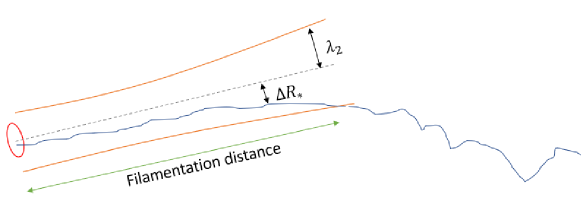
Figure 2: Schematic of the filamentation distance from the Sun, over which magnetic field lines can remain strongly trapped in filamentary flux tube structures. The solid blue curve represents a magnetic field line originating near an O-point in a magnetic island (red oval) near the solar surface. The orange curves depict the boundary of a nominal magnetic flux tube surrounding the corresponding O-line (dashed line) with radius equal to the bendover scale of 2D turbulence $\lambda_{2}$ (see text). The diffusion of the field line is suppressed over the filamentation distance, which is defined as the heliocentric distance at which the radial displacement $\Delta R_{\ast}$ of the field line from the O-point (base of the dashed grey line) becomes larger than $\lambda_{2}$. See also Figures 2 and 4 of Chuychai et al. (2007), which depict a similar physical process in numerical realizations of two-component magnetic turbulence.

To estimate a filamentation distance, instead of Equation (7) we solve a different ODE for field lines initially trapped in small-scale topological structures, accounting for the associated suppression of slab diffusion described above. Considering a magnetic field line distribution with spread $\langle\Delta R_{\ast}^{2}\rangle^{1/2}$ around a radius $R_{\ast}\sim\langle\Delta R_{\ast}^{2}\rangle^{1/2}$, i.e., a distribution spread near the O-point, we combine expansion and diffusion terms to obtain

$$\frac{d\langle\Delta R_{\ast}^{2}\rangle}{dz}=\frac{\langle\Delta R_{\ast}^{2}\rangle}{\mathscr{L}}+2D_{\perp}^{\text{slab}\ast},$$ (15)

where $D_{\perp}^{\text{slab}\ast}$ is given by Equation (14). We define the filamentation distance $r_{f}$ as the heliocentric distance corresponding to $z$ along the large-scale field line where $\langle\Delta R_{\ast}^{2}\rangle^{1/2}=\lambda_{2}$, the 2D bendover scale (see Figure 2), which is usually associated with the largest structures of 2D turbulence (Matthaeus et al., 2007). Note that a smaller initial $\langle\Delta R_{\ast}^{2}\rangle^{1/2}$ implies that field lines start closer to the center of an O-point, and consequently experience stronger trapping (as shown in Chuychai et al., 2007). In Appendix A we consider a piecewise power-law 2D spectrum (Matthaeus et al., 2007), and show that the 2D correlation scale $\lambda_{c2}$ can be related to the 2D bendover scale $\lambda_{2}$ by $\lambda_{c2}=\lambda_{2}(p+2)(\nu-1)/[(p+1)\nu]$, where $p$ is the low-wavenumber power-law index and $\nu$ is the inertial range power-law index. We choose $p=2$, the lowest value consistent with strict homogeneity of the two-point correlations, a property that may be questioned for the solar wind. Note, however, that Chhiber et al. (2017) found that the value of $p$ does not significantly influence energetic particle diffusion coefficients, so we adopt this value and defer further theoretical examination of this issue to a later time (see also Engelbrecht, 2019, and Appendix A). With $p=2$ and $\nu=5/3$ for a Kolmogorov inertial range, we obtain $\lambda_{c2}=0.53\lambda_{2}$. This relation may be used to compute $\lambda_{2}$ given $\lambda_{c2}$ from the turbulence transport model we employ, described below in Section 3.1.

To explain the significance of the filamentation distance, Figures 3(a)-(f) show results from Tooprakai et al. (2016), of magnetic field line tracing for a radial mean field superposed with a realization of 2D+slab turbulence in which an initial random-phase 2D field was processed through a 2D MHD simulation. Here 50,000 field lines were traced from initial positions at a radial distance of 0.1 au from the Sun, randomly distributed in heliolongitude $\varphi$ and heliolatitude $\Lambda$ within a circle of angular radius 2.5°. The different panels show $\varphi$ and $\Lambda$ of the same set of magnetic field lines at different values of the radial distance $r$. This models the distribution of magnetic connections to a compact region near the Sun, such as the region within which SEPs are injected by an impulsive solar flare into the interplanetary medium. Tooprakai et al. (2016) also confirmed by full orbital calculations that SEP trajectories closely follow the magnetic field line trajectories in this model (see also Laitinen et al., 2013; Laitinen & Dalla, 2017), and following previous reports (e.g., Giacalone et al., 2000; Ruffolo et al., 2003; Zimbardo et al., 2004), they associated the filamentary distribution of magnetic field-line connectivity with observations of “dropouts” of SEPs from impulsive solar flares.

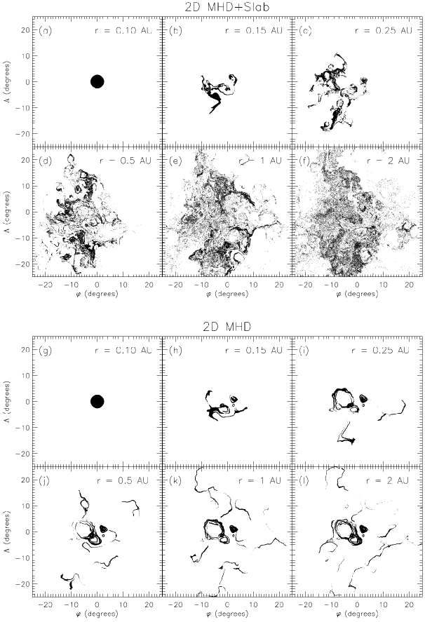
Figure 3: (a)-(f): Trajectories of field lines in heliolongitude and heliolatitude as a function of radius $r$ from the Sun, starting at random initial locations at r = 0.1 au within a circle of radius 2.5°, for a radial mean magnetic field superposed with a realization of 2D+slab magnetic turbulence, from Tooprakai et al. (2016). For this magnetic field, the calculated filamentation distance is 0.7 au, indicating a change from strong filamentation of field-line connectivity at $r<0.7$ au to a more diffusive spatial distribution, within a rather sharp outer envelope, at higher radius. Tooprakai et al. (2016) showed that the energetic-particle distribution closely follows the field-line distribution, so this models the spatial distribution of SEPs from impulsive solar flares. (g)-(l): Same, now removing the slab component of turbulence, i.e., for purely 2D MHD fluctuations. The difference in the field-line distribution confirms that slab fluctuations are crucial for defilamentation, i.e., for field lines to escape from 2D topological trapping and access wide regions within the overall angular spread of the FLRW.

For comparison, Figures 3(g)-(l) show our new results of field line tracing from the same initial positions for the same 2D magnetic field, but now without slab fluctuations. In this case of pure 2D fluctuations superposed on the radial mean field, the field line coordinates $\varphi(r)$ and $\Lambda(r)$ are constrained to conserve the 2D magnetic potential $a(\varphi,\Lambda)$ (Tooprakai et al., 2016). Thus, the angular coordinates $(\varphi,\Lambda)$ are constrained to remain on a single equipotential contour of $a$ (such contours are plotted in Figure 1(c) of Tooprakai et al., 2016). Level contours of 2D magnetic potential characteristically form closed 2D projections of flux tubes. Consequently the presence of a strong 2D turbulence component provides a template for restricting field line excursions and cross field particle transport. This strong constraint on FLRW makes it impossible for field lines to wander in a purely diffusive manner, and also implies that field lines from nearby initial positions usually remain close together, with strong concentrations of field line connectivity along narrow filaments and no connectivity with neighboring regions of space. While many of the field lines are trapped along small equipotential contours that remain near the initial positions, there are some equipotential contours that do extend over significant angular distances (up to $\sim 25\degree)$. Thus, even without slab turbulence, as $r$ increases out to 1 au, the rms angular spread of field lines continues to increase, but the slab turbulence component is crucial for defilamentation.

For the magnetic field in this 2D+slab simulation, we calculate the filamentation distance to be $r_{f}=0.7$ au. In Figures 3(b)-(c), where $r\ll r_{f}$, there is strong topological trapping of field lines and strong filamentation within a rms angular spread that increases with $r$. Then in Figures 3(d)-(f) where $r\sim r_{f}$ or is somewhat larger than $r_{f}$, there is some access of field lines (and energetic particles) to most angular regions (in a coarse-grained sense) within an outer envelope, and it is this less strongly filamented pattern, at or beyond the filamentation distance, that is qualitatively consistent with observed dropouts near Earth. Nevertheless, the spatial distribution of magnetic connectivity, or “dropout pattern,” remains substantially filamented at $r=1$ au, and indeed observations of dropouts confirm that 2D-like structures maintain substantial integrity to $r\approx 1$ au. Therefore, the lateral transport of field lines and energetic particles moving outward from the Sun to Earth orbit is not well described as diffusive. Furthermore, Figure 3 (as well as Figure 5 of Tooprakai et al., 2016) indicates a rather sharp outer boundary of the lateral transport that is inconsistent with a purely diffusive process.

Given the role of the slab component in disrupting filamentation, and presumably eventually leading to lateral diffusion at $r\gg 1$ au, we have defined the filamentation distance based on diffusion associated with the slab component. This slab diffusion is necessary to escape topological trapping near O-points of the 2D field, and is in turn suppressed by a strong 2D field, as described earlier in this section. This is why we chose to define $r_{f}$ as the distance where the field line displacement due to suppressed slab diffusion reaches the bendover scale of the 2D turbulence.

3 Solar Wind Model with Turbulence Transport

To evaluate the rms displacement of heliospheric magnetic field lines using the formalism developed in the previous Section, we must specify both the large-scale magnetic field and the field-line diffusion coefficient, the latter of which requires quantifying the smaller-scale turbulence properties along the field line. We emphasize that the formalism of Section 2 can be quite generally used with any model that provides the requisite inputs. In this section we briefly describe the MHD solar wind model that we employ here to supply the requisite information. We also provide details on the numerical implementation. Note that an earlier version of this model was recently used by Chhiber et al. (2017) to compute 3D distributions of energetic-particle diffusion coefficients throughout the inner heliosphere.

3.1 Model Description

The two-fluid MHD coronal and heliospheric model that we employ is described in detail in Usmanov et al. (2014) and Usmanov et al. (2018). The model is based on the Reynolds-averaging approach (e.g., McComb, 1990): a physical field, e.g., $\tilde{\bm{a}}$, is separated into a mean and a fluctuating component: $\tilde{\bm{a}}=\bm{a}+\bm{a}^{\prime}$, making use of an ensemble-averaging operation where $\bm{a}=\langle\tilde{\bm{a}}\rangle$ and, by construction, $\langle\bm{a}^{\prime}\rangle=0$. Application of this Reynolds decomposition to the underlying primitive compressible MHD equations, along with a series of approximations appropriate to the solar wind, leads us to a set of mean-flow equations that are coupled to the small-scale fluctuations via another set of equations for the statistical descriptors of the unresolved turbulence.

To derive the mean-flow equations, the velocity and magnetic fields are Reynolds-decomposed: $\tilde{\bm{v}}=\bm{v}+\bm{v^{\prime}}$ and $\widetilde{\bm{B}}=\bm{B}+\bm{B^{\prime}}$, and then substituted into the momentum and induction equations in the frame of reference corotating with the Sun. The ensemble averaging operator $\langle\dots\rangle$ is then applied to these two equations (Usmanov et al., 2014, 2018). The resulting mean-flow model consists of a single momentum equation and separate ion and electron temperature equations, in addition to an induction equation. Density fluctuations are neglected, and pressure fluctuations are only those required to maintain incompressibility (Zank & Matthaeus, 1992). The Reynolds-averaging procedure introduces additional terms in the mean flow equations, representing the influence of turbulence on the mean (average) dynamics. These terms involve the Reynolds stress tensor $\bm{\mathcal{R}}=\langle\rho\bm{v}^{\prime}\bm{v}^{\prime}-\bm{B}^{\prime}\bm{B}^{\prime}/4\pi\rangle$, the mean turbulent electric field $\mathcal{\bm{\varepsilon}}_{m}=\langle\bm{v}^{\prime}\times\bm{B}^{\prime}\rangle(4\pi\rho)^{-1/2}$, the fluctuating magnetic pressure $\langle B^{\prime 2}\rangle/8\pi$, and the turbulent heating, or “heat function” $Q_{T}(\bm{r})$, which is apportioned between protons and electrons. Here the mass density $\rho=m_{p}N_{S}$ is defined in terms of the proton mass $m_{p}$ and number density $N_{S}$. The pressure equations employ the natural ideal gas value of 5/3 for the adiabatic index. The pressure equations also include weak proton-electron collisional friction terms involving a classical Spitzer collision time scale $\tau_{SE}$ (Spitzer, 1965; Hartle & Sturrock, 1968) to model the energy exchange between the protons and electrons by Coulomb collisions (see Breech et al., 2009). We neglect the heat flux carried by protons; the electron heat flux ($\mathbf{q}_{E}$) below $5\text{ -- }10~{}\text{R}_{\odot}$ is approximated by the classical collision-dominated model of Spitzer & Härm (1953) (see also Chhiber et al., 2016), while above $5\text{ -- }10~{}\text{R}_{\odot}$ we adopt Hollweg’s “collisionless” conduction model (Hollweg, 1974, 1976). See Usmanov et al. (2018) for more details.

Closure of the above system requires a model for unresolved turbulence. Although the Reynolds decomposition is not formally a scale separation, we have in mind that the stochastic components treated as fluctuations reside mainly at the relatively small scales, i.e., comparable to, or smaller than, the correlation scales. Transport equations for the fluctuations may be obtained by subtracting the mean-field equations from the full MHD equations and averaging the difference (see Usmanov et al., 2014). This yields a set of three equations (Breech et al., 2008; Usmanov et al., 2014, 2018) for the chosen statistical descriptors of turbulence, namely $Z^{2}=\langle v^{\prime 2}+b^{\prime 2}\rangle$, i.e., twice the fluctuation energy per unit mass where $\bm{b}^{\prime}=\bm{B}^{\prime}(4\pi\rho)^{-1/2}$; the normalized cross helicity, $\sigma_{c}=2\langle\bm{v}^{\prime}\cdot\bm{b}^{\prime}\rangle/Z^{2}$, or normalized cross-correlation between velocity and magnetic field fluctuations; and $\lambda$, a correlation length perpendicular to the mean magnetic field. Other parameters include the normalized energy difference, which we treat as a constant parameter ($=-1/3$) derived from observations (see also Zank et al., 2017), and the Kármán-Taylor constants (see Matthaeus et al., 1996; Smith et al., 2001; Breech et al., 2008).

Note that the fluctuation energy loss due to von Kármán decay (de Kármán & Howarth, 1938; Hossain et al., 1995; Wan et al., 2012; Wu et al., 2013; Bandyopadhyay et al., 2018) is balanced in a quasi-steady state by internal energy supply in the pressure equations. To evaluate the Reynolds stress we assume that the turbulence is transverse to the mean field and axisymmetric about it (Oughton et al., 2015), so that we obtain $\bm{\mathcal{R}}/\rho=K_{R}(\bm{I}-\hat{\bm{B}}\hat{\bm{B}})$, where $K_{R}=\langle v^{\prime 2}-b^{\prime 2}\rangle/2=\sigma_{D}Z^{2}/2$ is the residual energy and $\hat{\bm{B}}$ is a unit vector in the direction of $\bm{B}$. The turbulent electric field is neglected here. For further details see Usmanov et al. (2018).

3.2 Numerical Implementation

We solve the Reynolds-averaged mean-flow equations concurrently with the turbulence transport equations in the spherical shell between the base of the solar corona (just above the transition region) and the heliocentric distance of 5 au. The computational domain is split into two regions: the inner (coronal) region of $1\text{ -- }30~{}\text{R}_{\odot}$ and the outer (solar wind) region from $30~{}\text{R}_{\odot}\text{ -- }5$ au. The relaxation method, i.e., the integration of time-dependent equations in time until a steady state is achieved, is used in both regions.

The model is well tested and provides reasonable agreement with both in-situ and remote observations (Usmanov et al., 2011, 2012, 2014; Chhiber et al., 2017, 2018; Usmanov et al., 2018; Chhiber et al., 2019; Bandyopadhyay et al., 2020; Ruffolo et al., 2020). The simulations used have typically been of two major types, distinguished by the inner surface magnetic boundary condition: In the first type a Sun-centered dipole magnetic field is imposed at the inner boundary, with a specified tilt angle relative to the solar rotation axis. Zero or small tilt angle is often associated with solar activity minimum, while larger tilt angles are a suitable approximation for the more disordered heliosphere during solar maximum conditions (Owens & Forsyth, 2013). The second kind of inner magnetic boundary condition is based on suitably normalized magnetograms (Riley et al., 2014; Usmanov et al., 2018).

In the present paper we employ two runs: A dipole-based run with a tilt of 10° relative to the solar rotation axis, toward 330° longitude (Run I), and a Carrington Rotation (CR) 2123 magnetogram-based run representative of solar maximum conditions (Run II), during the time period 2012 April 28 to 2012 May 25. The CR 2123 magnetogram from Wilcox Solar Observatory was scaled by a factor of 8 and smoothed using a spherical harmonic expansion up to 9th order. Run I has a resolution of $702\times 120\times 240$ along $r\times\theta\times\phi$ coordinates. The computational grid has logarithmic spacing along the radial ($r$) direction, with the grid spacing becoming larger as $r$ increases. The latitudinal ($\theta$) and longitudinal ($\phi$) grids have equidistant spacing, with a resolution of 1.5° each. Run II has a resolution of $154\times 60\times 120$ in the inner (coronal) region, and a resolution of $400\times 120\times 240$ in the outer region.

Figure 4: Panels (a)-(d) show global simulation results for the mean magnetic-field strength $B$, proton number density $n$, turbulence energy $Z^{2}$, and the correlation scale $\lambda$, respectively, in a meridional plane at 1° heliolongitude and heliocentric distances of $1\text{ -- }215~{}\text{R}_{\odot}$, from Run I. These quantities are used to compute the field line diffusion coefficients $D_{\perp}^{\text{slab}}$ and $D_{\perp}^{\text{2D}}$ using Equations (9) and (11), and the suppressed slab diffusion coefficient $D_{\perp}^{\text{slab}\ast}$ [Equation (14)], shown in panels (e)-(g), respectively. Panel (h) shows the ratio $D_{\perp}^{\text{slab}\ast}/D_{\perp}^{\text{slab}}$.

The input parameters specified at the coronal base include: the driving amplitude of Alfvén waves (30 km s^-1), the density ($1\times 10^{8}$ particles cm^-3), the correlation scale of turbulence ($10,500$ km), and temperature ($1.8\times 10^{6}$ K). The cross helicity in the initial state is set as $\sigma_{c}=-\sigma_{c0}B_{r}/B_{r}^{\text{max}}$, where $\sigma_{c0}=0.8$, $B_{r}$ is the radial magnetic field, and $B_{r}^{\text{max}}$ is the maximum absolute value of $B_{r}$ on the inner boundary. The magnetic field magnitude is assigned using a source magnetic dipole (with strength 12 G at the poles to match values observed by Ulysses). The input parameters also include the fraction of turbulent energy absorbed by protons $f_{p}=0.6$. Further details on the numerical approach and initial and boundary conditions may be found in Usmanov et al. (2018).

4 Results

We begin this section by presenting a sample of the global simulation results that we use to evaluate field line diffusion: the large-scale magnetic field magnitude $B$, proton density $n$, turbulence energy $Z^{2}$, and correlation scale $\lambda$. Figures 4(a)-(d) show sample results from Run I in a meridional plane at 1° heliolongitude, in heliographic coordinates (HGC; Fränz & Harper, 2002). The heliospheric current sheet (HCS) is clearly visible at low-latitudes in panel (a), and it is also a region of relatively high density, as expected for low-latitude slow wind during solar minimum (McComas et al., 2000). The turbulence quantities also exhibit interesting (and expected) latitudinal variation. Mid-to-high latitude fast wind is more Alfvénic, with higher turbulence energy relative to lower latitudes at the same radial distance. As expected the turbulence energy density decreases with radius almost everywhere. On the other hand, the correlation scale increases with distance from the Sun as the turbulence “ages” and the inertial-range cascade extends to larger spatial scales (Matthaeus et al., 1998; Bruno & Carbone, 2013; DeForest et al., 2016; Chhiber et al., 2018), with the more turbulent slow-wind ageing faster. For more detailed description of the base variables from the simulation see Usmanov et al. (2018).

Next, to evaluate the field line diffusion coefficients according to Equations (9), (11), and (14), we make some approximations that are appropriate to the inner heliosphere, for estimating the slab and 2D fractions of turbulent energy and correlation scales. First, we note that the turbulent fluctuations in our model are primarily transverse to the mean magnetic field (Breech et al., 2008; Usmanov et al., 2014, 2018), while in addition the quasi-2D contribution to the energy is generally the dominant contribution. Therefore we associate the correlation scale of the 2D turbulence with the dynamically evolving similarity scale $\lambda$ in our turbulence model, so that $\lambda_{\text{c2}}=\lambda$. Observational studies indicate that the slab correlation scale is about a factor of two larger than the 2D correlation scale (Osman & Horbury, 2007; Weygand et al., 2009, 2011), and accordingly, we assume $\lambda_{\text{slab}}=2\lambda_{\text{c2}}$. Next, we assume that the slab fraction of the total magnetic fluctuation energy $\langle B^{\prime 2}\rangle$ is $f_{s}=0.2$, a decomposition that is well supported both theoretically (Zank & Matthaeus, 1992, 1993; Zank et al., 2017) and observationally (Matthaeus et al., 1990; Bieber et al., 1994, 1996). Then we have $b^{2}_{\text{s}}=f_{\text{s}}\langle B^{\prime 2}\rangle$ and $b^{2}_{\text{2D}}=(1-f_{\text{s}})\langle B^{\prime 2}\rangle$. Finally, we convert $Z^{2}$ from the simulation to $\langle B^{\prime 2}\rangle$ using the relation $\langle B^{\prime 2}\rangle=4\pi\rho Z^{2}/(r_{\text{A}}+1)$ (see Section 3.1), and an Alfvén ratio $r_{\text{A}}=\langle{v^{\prime}}^{2}\rangle/\langle{b^{\prime}}^{2}\rangle=1/2$ is assumed (Tu & Marsch, 1995).

Using the above approximations, we are able to compute all parameters required to evaluate the diffusion coefficients, based on the dynamically evolved turbulence parameters provided by the subgrid turbulence model in the Usmanov et al. global MHD code. 2D maps of the field line diffusion coefficients in meridional planes at 1° heliolongitude are shown in panels (e)-(g) of Figure 4. We see that $D_{\perp}$ increases with distance from the Sun, and is relatively larger in the slow-wind region around the HCS. The suppressed slab diffusion coefficient $D_{\perp}^{\text{slab}\ast}$ behaves similarly. It is interesting to examine the ratio $D_{\perp}^{\text{slab}\ast}/D_{\perp}^{\text{slab}}$ in panel (g), which reveals that there is significant suppression of slab diffusion for trapped field lines at all latitudes, with the strongest effect seen near the HCS.

With all the quantities needed to solve Equations (7) and (15) in place, we next trace magnetic field lines from the coronal base out to 1 au, employing trilinear interpolation of the relevant quantities ($B\equiv B_{0},D_{\perp}$, and $D_{\perp}^{\text{slab}\ast}$) to the field line under consideration. The ODEs are then integrated along the large-scale field line using a second-order Runge-Kutta method to evaluate the mean-squared spread of field lines $\langle\Delta R^{2}\rangle$, with an initial spread corresponding to a circle of radius 2° at 0.1 au. To estimate the filamentation distance and the associated “suppressed” spreading, we integrate Equation (15) with different values of initial $\langle\Delta R_{\ast}^{2}\rangle$, which represent varying initial rms displacements of field lines from the center of an O-point. We also vary the slab fraction $f_{s}$ of the magnetic fluctuation energy. Stronger trapping is expected for smaller values of initial displacement and $f_{s}$ (see Section 2.3). A three-point Lagrangian interpolation formula (e.g., Hildebrand, 1974) is used to approximate the derivative of $B_{0}$ along $z$. In the following two subsections we describe the results obtained in this way from Runs I and II. In the following, longitude (latitude) is used interchangeably with heliolongitude (heliolatitude), referring to HGC coordinates.

4.1 Run I: Dipole-based Simulation

We recall that Run I is a dipole-based run ($1~{}R_{\sun}\text{ -- }5$ au) with the dipole axis tilted by 10° relative to the solar rotation axis. Integration of Equations (7) and (15), with a starting spread corresponding to a circle of given radius at 0.1 au provides values for the rms transverse displacement $\langle\Delta R^{2}\rangle^{1/2}$ and rms suppressed slab displacement $\langle\Delta R_{\ast}^{2}\rangle^{1/2}$, as described in Sections 2.2 and 2.3. The latter quantity is relevant to the spread of field lines initially trapped in small-scale topological structures where slab diffusion is suppressed.

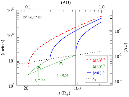
Figure 5: Results from Run I, a global simulation for a solar magnetic dipole with 10° tilt, showing the 2D bendover scale $\lambda_{2}$ (dotted black curve), normal FLRW spread $\langle\Delta R^{2}\rangle^{1/2}$ (dashed red curve), suppressed spread $\langle\Delta R_{\ast}^{2}\rangle^{1/2}$ (solid green curves), and spread after escape from trapping boundary $\langle\Delta\mathscr{R}^{2}\rangle^{1/2}$ (solid blue curves), along a field line that originates at 55° latitude and 0° longitude. The latter two quantities are shown for two values of slab energy fraction – $f_{s}=0.2$ and $f_{s}=0.02$, with initial $\langle\Delta R_{\ast}^{2}\rangle^{1/2}$ corresponding to $2.7\times 10^{8}$ m. Vertical grey lines indicate the filamentation distance for the two cases, at $42~{}\text{R}_{\odot}$ and $95~{}\text{R}_{\odot}$, respectively. For the calculation of normal FLRW spread $\langle\Delta R^{2}\rangle^{1/2}$, $f_{s}=0.2$.

Figure 5(a) shows the above two quantities for a field line that originates at 55° latitude and 0° longitude. Here an initial spread corresponding to a circle of radius 2° is used for evaluating $\langle\Delta R^{2}\rangle^{1/2}$, while an intial spread of 1° is used for evaluating $\langle\Delta R_{\ast}^{2}\rangle^{1/2}$. Also shown is the 2D bendover scale $\lambda_{2}$. The filamentation distance $r_{f}$ (vertical grey line) is the heliocentric distance at which $\langle\Delta R_{\ast}^{2}\rangle^{1/2}=\lambda_{2}$, the 2D bendover scale. Beyond this point, field lines that are initially trapped can begin to undergo an unsuppressed random walk. We also show $\langle\Delta\mathscr{R}^{2}\rangle^{1/2}$, which represents the spreading of field lines after they have escaped trapping boundaries (see schematic in Figure 2). This quantity is obtained by integrating the normal FLRW equation [Equation (7)], starting at the filamentation distance $r_{f}$ with an initial spread equal to the value of $\langle\Delta R_{\ast}^{2}\rangle^{1/2}$ at $r_{f}$. Note that we only show mid-latitude field lines from Run I since all low-latitude field lines close back onto the solar surface for the dipolar-source magnetic field; however, even such mid-latitude field lines can meander to the ecliptic plane, as discussed below. Field lines originating at low latitude may be obtained from the magnetogram-based Run II (see Section 4.2, below).

The results in Figure 5 show an rms spread of around 3-6 $\times 10^{10}$ m at 1 au for both regular, untrapped field lines and for those that are initially trapped. The latter experience significantly reduced diffusion up to the filamentation distance ($42~{}\text{R}_{\odot}$ and $95~{}\text{R}_{\odot}$ for the two slab fractions shown), and then begin to approach the outer envelope. The corresponding angular spreads near Earth are around 25°. Note that the angular spread refers to the angle subtended by the radius of rms diffusive spreading at a distance of 1 au. Therefore the separation in longitude between two field lines that have random walked in opposite directions can be $\sim 50\degree$ (see also Section 4.2). These spreads are consistent with those inferred from observations of SEPs from some impulsive solar events (e.g., Wibberenz & Cane, 2006; Wiedenbeck et al., 2013; Dröge et al., 2014) and from full particle orbit simulations by Tooprakai et al. (2016) (see also Figure 3). It is interesting to note that Laitinen et al. (2016) find a similar angular spread of SEPs in the distance range of 0.5 to 1.5 au, in a calculation in which it is shown that the FLRW makes a substantial contribution, although in that case the field line spread is entirely of a diffusive nature.

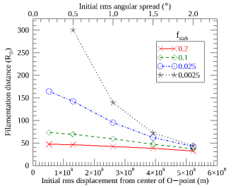
Figure 6: Parameter study for calculation of filamentation radius $r_{f}$ for a field line from the tilted-dipole simulation (Run I), at initial latitude and longitude of 55° and 0°, respectively. The figure shows $r_{f}$ for different values of slab-energy fraction $f_{s}$ and varying initial rms displacement from the center of the O-point [i.e., initial $\langle\Delta R_{\ast}^{2}\rangle^{1/2}$ in Equation (15)], for the case of field lines initially trapped in a magnetic island.

As we have calculated it, the filamentation distance is explicitly dependent on the amplitude of slab fluctuations present in the turbulence. In addition, we recall that Chuychai et al. (2007) found that the suppressed diffusive-escape theory matches simulations best for small slab fraction (0.001-0.0025), i.e., when the 2D component is dominant (see Figures 8 and 9 of Chuychai et al., 2007). It is therefore of interest to examine, within the context of that theory, how the filamentation distance varies in the present framework, as one varies the slab fraction and the distance of a field line from the central O-point in a flux tube. A brief parameter study of these effects is illustrated in Figure 6. Here the initial displacement from the O-point is varied from 5 $\times 10^{7}$ m to 5.2 $\times 10^{8}$ m, and the slab fraction is varied from 0.0025 to 0.2 of the total magnetic fluctuation energy. For each value of the slab fraction the filamentation distance monotonically increases as the field line’s initial position is migrated closer to the O-point (see also Figure 5 of Chuychai et al., 2007). In addition, there is a dramatic increase in filamentation distance for smaller slab fractions.

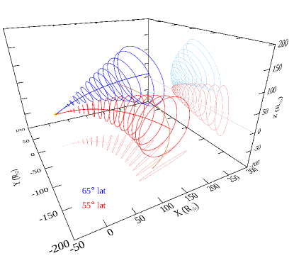
Figure 7: 3D representation of two field lines originating at 65° and 55° latitude, and 0° longitude, traced from the coronal base at $1~{}\text{R}_{\odot}$ to the distance of Earth orbit (depicted nominally as a brown curve) for global simulation Run I. The circles around the central field lines have a radius equal to $\langle\Delta R_{\ast}^{2}\rangle^{1/2}$ from 0.1 au up to the filamentation distance and a radius $\langle\Delta\mathscr{R}^{2}\rangle^{1/2}$ beyond that. The projections of the 55° case on the X-Y and Y-Z planes, and a projection of the 65° case on the Y-Z plane, are shown in muted colors. The light-grey line in the Y-Z plane marks Z=0 for reference. The axes represent HGC coordinates.

Figure 8: Results from Run II, a global simulation based on a CR 2123 magnetogram. (a) 2D bendover scale $\lambda_{2}$ (dotted black curve), normal FLRW spread $\langle\Delta R^{2}\rangle^{1/2}$ (dashed red curve), suppressed spread $\langle\Delta R_{\ast}^{2}\rangle^{1/2}$ (solid green curve), and spread after the end of suppression $\langle\Delta\mathscr{R}^{2}\rangle^{1/2}$ (solid blue curves), along a field line that originates at 1° latitude and 69° longitude. The latter two quantities are shown for two values of slab energy fraction – $f_{s}=0.2$ and $f_{s}=0.02$, with initial $\langle\Delta R_{\ast}^{2}\rangle^{1/2}$ corresponding to $2.7\times 10^{8}$ m. Vertical grey lines indicate the filamentation distance for the two cases, at $44~{}\text{R}_{\odot}$ and $120~{}\text{R}_{\odot}$, respectively. For the calculation of normal FLRW spread $\langle\Delta R^{2}\rangle^{1/2}$, $f_{s}=0.2$. (b) Angular spread of two selected field lines as a function of heliocentric distance. The 1° and -9° latitude fieldlines originate at 69° and 159° longitude, respectively. The rms angular spread is computed as $\theta=\langle\Delta R^{2}\rangle^{1/2}/r$, where $r$ is the radial coordinate of a field line.

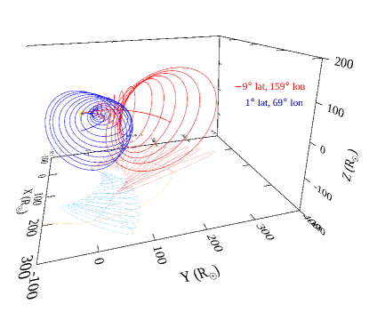
Figure 9: 3D representation of two field lines originating at latitude/longitude of 1°/69° (blue) and -9°/159° (red), traced from the coronal base at $1\text{R}_{\odot}$ to the distance of a nominal Earth orbit (depicted as a pale brown curve in the X-Y plane projection), from global simulation Run II. The circles around the central field lines have a radius equal to $\langle\Delta R_{\ast}^{2}\rangle^{1/2}$ from 0.1 au up to the filamentation distance, and a radius $\langle\Delta\mathscr{R}^{2}\rangle^{1/2}$ beyond that. The projections of the field lines on the X-Y plane are shown in muted colors. The axes represent HGC coordinates.

Figure 7 shows a 3D representation of two field lines, from the solar surface to Earth orbit (depicted as a brown curve). The circles around the central field lines have a radius equal to $\langle\Delta R_{\ast}^{2}\rangle^{1/2}$ from 0.1 au up to the filamentation distance, and a radius $\langle\Delta\mathscr{R}^{2}\rangle^{1/2}$ above it. At 1 au, the rms separation of random-walking field lines can be in excess of $100~{}\text{R}_{\odot}$. Further, one observes from the Y-Z projection of the field line originating at 55° latitude, that field lines originating from solar mid-latitudes can meander to the ecliptic by their arrival at 1 au. The projection of the two field lines on the Y-Z plane shows that there can be mixing between field lines originating at different latitudes. The next subsection shows a similar figure for the case of the magnetogram-based simulation.

4.2 Run II: Magnetogram-based Simulation

In this subsection we present results from Run II, which employs a magnetogram corresponding to CR 2123 (2012 April 28 – 2012 May 25), a period of high solar activity. Due to the more complex and more realistic magnetic field produced by the magnetogram initialization, it is of interest to consider two problems: First we will integrate outward to 1 au from a specified source region, as in the previous section. Next, we will begin an integration at 1 au and integrate inward along a large-scale field line to infer a broader area that represents a possible source region.

To begin, as in the dipolar case, we integrate Equations (7) and (15) starting at 0.1 au, with a specified initial spread corresponding to a circle of radius 2° (1° for the case of suppressed spread). Results based on this run are shown in Figures 8 – 9. Note that in this case we are able to examine field lines originating at low latitudes, in contrast to the dipole run wherein all low-latitude field lines close back onto the solar surface.

The results are qualitatively similar to those in the previous subsection, but the rms spreads are almost a factor of two larger, possibly owing to stronger fluctuations during solar maximum. It is noteworthy that in this magnetogram-driven case, the typical angular spread of field lines at 1 au from the source can exceed 50° [see Figure 8(b)]. Likewise, examining Figure 9, it is possible to observe an rms separation of field lines at 1 au that is in excess of 200 Earth radii. Figure 9 also shows that mixing can occur between field lines originating at widely separated ($\sim 90\degree$) longitudes, due to FLRW.

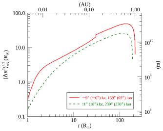
Figure 10: The reverse FLRW spread $\langle\Delta R^{2}\rangle^{1/2}_{\text{rev}}$ of selected field lines from global simulation Run II, assuming an initial spread of zero at 1 au and integrating the FLRW equation (7) Sunward. The solid red and dashed green curves show the rms spread around field lines that originate at latitude/longitude of $-9\degree/159\degree$  and 11°/239° near the solar surface, and at 1 au have a latitude/longitude of $-6\degree/69\degree$  and $18\degree/230\degree$, respectively.

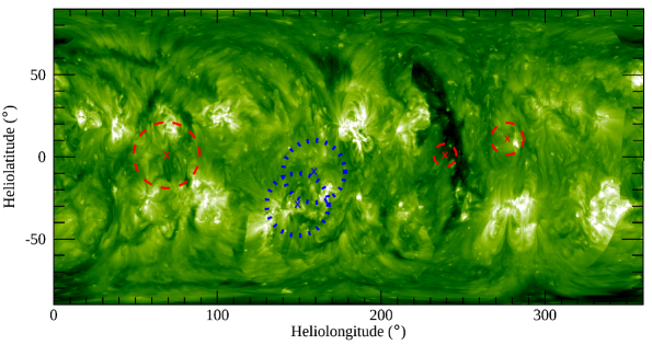
Figure 11: Synoptic map of the solar corona dated 2012 May 12, during CR 2123. The synchronized EUV image is based on STEREO/EUVI A and B 195 Å and SDO/AIA 193 Å observations. The processing involved in producing this image is described in Caplan et al. (2016). From our global simulation Run II based on a CR 2123 magnetogram, we calculate the reverse spread of field lines connected to specific locations at 1 au from the Sun, as described in the text. The blue and red ‘$\times$’ symbols mark the origins of selected field lines in low-latitude regions with positive and negative polarities, respectively. The circles (dashed red for negative and dotted blue for positive polarities) have radii equal to $\langle\Delta R^{2}\rangle^{1/2}_{\text{rev}}$ at the solar surface, and mark regions from which a field line, at the position at 1 au corresponding to that of the central ‘$\times$’ field line, is likely to have originated. We show that because of turbulent fluctuations, there can be a significant uncertainty in back-tracing of field lines from 1 au. The synoptic map was obtained from http://www.predsci.com/chd/.

Turning the problem around, and integrating inward, it is possible to investigate the extent of the spatial region on the solar surface from which a field line localized at 1 au could have originated. For this purpose we integrate the FLRW equation (7) Sunward, assuming an initial spread of zero at 1 au. In Figures 10 and 11 we show the results of this computation of the reverse FLRW for selected field lines. One observes that the region of likely field line spreading extends over regions comparable to the large features on the solar synoptic map, on the order of the supergranulation scale of $\sim$ 35,000 km, or even larger. Thus we see that turbulent fluctuations can induce a significant uncertainty (around 20° in latitude/longitude) in any sort of back-tracing of field lines to the solar surface. Field line random walk due to unresolved fluctuations introduces an inherent inaccuracy in determination of the location on the Sun that is magnetically connected to a location of interest at distance $\sim$ 1 au. This translates directly into uncertainty in identifying coronal sources of solar wind plasma and energetic particles.

5 Discussion

The purpose of this paper has been to develop methods for approximating the spread of magnetic field lines in an inhomogeneous expanding medium such as the solar wind, and to implement that method employing data from a global heliospheric MHD model. The framework developed combines two contributors to magnetic field line spread. The first, a coherent effect, is due to expansion of the large-scale or resolved field, for which an explicit representation is available, e.g., from a global simulation. The second effect included is the random influence on spreading due to unresolved turbulence that is known only in terms of its statistical properties such as its spectrum. The latter effect requires a theoretical model for how turbulence descriptors such as the variance and correlation scale vary along the resolved field line that is traced. Here we employ one particular approach for this step, namely implementing and solving a set of turbulence transport equations for turbulence energy and correlation scale that are self-consistently solved along with the large scale resolved “macro” MHD model (Usmanov et al., 2018). Taken together, the approximate treatment of this problem that is developed in Section 2 provides a fairly general framework for approximating the spread of magnetic field lines in a variety of problems. The main motivation here is the tracing of connectivity from solar sources to interplanetary space and vice versa. This has potential important implications for solar energetic particle propagation, as well as space weather applications.

In particular, embedding the above formalism into a global model that supplies both large scale magnetic fields and turbulence parameters comprises an approach that shows promise in incorporating a degree of realism into quantifying field line connectivity and transport of SEPs. We are aware that some prior studies have evaluated the impact of field line meandering on particle transport, and concluded that the impact is minimal. Nolte & Roelof (1973) provide a concise summary of several such studies, in each case finding no support for spreading due to FLRW in observations. One such line of reasoning argues that field line meandering due to photospheric motions has sometimes been overestimated (Nolte & Roelof, 1973; Kavanagh et al., 1970). In this regard we note that the time dependent boundary effect alluded to in this argument is actually distinct from our starting point, which is the standard static FLRW that emerges from spatially distributed fluctuations without relying on any specific boundary variations in time (however, see Giacalone et al., 2006, for boundary models for generation of fluctuations). More direct observational limits on transverse diffusion have also been reported based on multiple point observations of SEPs (Krimigis et al., 1971). This conclusion is largely based on examples of observations in which intensity profiles remain relatively intact over significant distances. It is not possible to discount such reports; however, we have seen that SEPs can indeed remain concentrated within trapping structures for relatively large distances, in some cases as far as 1 au. This phenomenon has been argued to be the basis for observed dropouts, which we attribute to topological trapping that delays the transition to standard diffusion. In the present study this effect is incorporated into the model by defining the filamentation distance, a quantity that provides an estimate of the typical distance over which this trapping occurs. Further quantitative observational study will be needed to ascertain the accuracy of the present theoretical framework.

The results of the implementation of our framework within the global solar wind model are summarized below. We find rms spreads at 1 au of about $10^{10}$ - $10^{11}$ m, which correspond to rms angular spreads of about 20° - 60°; these estimates are generally consistent with the turbulence simulations of Tooprakai et al. (2016). The spreading is generally larger in the magnetogram-driven simulation corresponding to solar maximum, compared with the 10° dipole-tilt simulation. Note that this rms spreading implies that random-walking field lines originating within the same source region can develop separations as wide as 120° in longitude. Thus, our framework can account for the wide spreads that are sometimes seen in impulsive SEP observations (e.g., Wibberenz & Cane, 2006; Wiedenbeck et al., 2013; Dröge et al., 2014). We also evaluate the heliocentric distances up to which field lines originating in magnetic islands can remain strongly trapped; depending on the fraction of slab energy in the magnetic turbulence, and the initial distance from the center of the trapping island; this “filamentation distance” is estimated to be between 40 - $150~{}\text{R}_{\odot}$, which is again consistent with Tooprakai et al. (2016). Finally, we estimate the uncertainty in magnetic connectivity of 1 au observations to solar sources; this is found to be around 20° in latitude/longitude at the source.

In closing, we emphasize that there is a reasonable degree of generality in the formalism developed here in Section 2, and that it may be employed within other global solar wind models and large-scale or global models of other astrophysical systems for which the required turbulence parameters can be deduced. To facilitate applications, Appendix B provides an implementation of our theoretical approach based on an extremely simplified empirical treatment of the required parameters describing the magnetic field. Results of that exercise are illustrated in Figure 12.

Although this approach may be adapted rather directly to different applications, we should recall that this theoretical development is approximate, given simplifications such as the neglect of correlations between the deflections due to large-scale expansion and the deflections due to the modeled small-scale turbulence. It may be of particular interest to extend this approach to the outer heliosphere and the very local interstellar medium, locations where field line connectivity may be relevant to explaining observations by Voyager, IBEX, and the upcoming IMAP missions (McComas et al., 2018; Zank et al., 2019; Zirnstein et al., 2020; Fraternale et al., 2020).

Appendix A Relating the 2D Correlation Scale to the 2D Bendover Scale

To obtain a relationship between the 2D bendover scale $\lambda_{2}$ and the 2D correlation scale $\lambda_{\text{c2}}$ (see Section 2.3), we begin with the following form for the 2D modal power spectrum (Matthaeus et al., 2007):

$$S_{2}(k_{\perp})=\left\{\begin{array}[c]{l}C_{2}\langle b_{\text{2D}}^{2}\rangle\lambda_{2}^{2}(\lambda_{2}k_{\perp})^{p},\\ C_{2}\langle b_{\text{2D}}^{2}\rangle\lambda_{2}^{2}(\lambda_{2}k_{\perp})^{-\nu-1},\end{array}\right.\begin{array}[c]{l}\text{if }k_{\perp}\leq 1/\lambda_{2},\\ \text{if }k_{\perp}>1/\lambda_{2},\end{array}$$ (A.1)

where $C_{2}$ is a dimensionless constant, $k_{\perp}$ is a 2D wavenumber, and $p$ is a power-law index that determines the long-wavelength behavior of the spectrum. We also assume that the inertial range power-law index is $\nu=5/3$, leading to an omnidirectional spectrum ${\cal E}(k_{\perp})=2\pi k_{\perp}S_{2}(k_{\perp})\propto k_{\perp}^{-5/3}$ that is consistent with Kolmogorov theory. In the present work we assume $p=2$, the lowest value that is consistent with strict homogeneity. We remark here that Chhiber et al. (2017) found that the value of $p$ did not significantly influence energetic particle diffusion coefficients; however, if one uses a form for the spectrum with three separate wavenumber ranges (Matthaeus et al., 2007), then the diffusion coefficients may be sensitive to the choice for $p$ (see Engelbrecht, 2019).

The constant $C_{2}$ may be determined by the normalization condition $\langle b_{\text{2D}}^{2}\rangle=2\pi\int_{0}^{\infty}S_{2}(k_{\perp})k_{\perp}dk_{\perp}$, yielding $C_{2}=(\nu-1)(p+2)/[2\pi(p+\nu+1)]$. Next, we use the expression for the 2D correlation scale (Equation (10) of Matthaeus et al., 2007):

$$\lambda_{\text{c2}}=\frac{\int[S_{2}(k_{\perp})/k_{\perp}]dk_{x}dk_{y}}{\langle b^{2}_{\text{2D}}\rangle}=2\pi\frac{\int_{0}^{\infty}S_{2}(k_{\perp})dk_{\perp}}{\langle b^{2}_{\text{2D}}\rangle}.$$ (A.2)

On substituting the spectrum from Equation (A.1) into the above and carrying out the integration, we obtain

$$\lambda_{\text{c2}}=\lambda_{2}\frac{(p+2)(\nu-1)}{(p+1)\nu},$$ (A.3)

which yields $\lambda_{\text{c2}}=0.53\lambda_{2}$ on choosing $p=2$ and $\nu=5/3$.

Appendix B Estimates of FLRW using simplified turbulence scalings

To expand the applicability of our formalism to solar wind models that do not include a turbulence transport component, in this appendix we use simple approximations for turbulence parameters to obtain the FLRW diffusion coefficient. These approximations are (1) constant $b/B_{0}$, and (2) the widely used Hollweg (1986) prescription for the turbulence correlation scale: $\lambda\propto 1/B_{0}^{1/2}$. Here $b$ and $B_{0}$ are the rms magnetic fluctuation strength and the mean magnetic field, respectively. The Hollweg correlation scale is identified with the 2D turbulence. In Figure 12 the diffusion coefficient based on these approximations (and the corresponding rms spread of field lines) is compared with calculations based on the turbulence transport model. All calculations use $B_{0}$ from the global solar wind simulation described in Section 3.

Figure 12: (a) Ratio of FLRW diffusion coefficients $D_{\perp}/D^{\prime}_{\perp}$, where $D_{\perp}$ is computed from the turbulence transport model and $D^{\prime}_{\perp}$ using the simple approximations described in Appendix B. The figure shows the radial evolution of this ratio for two field lines at latitudes of 7° and 82°, at a longitude of 0°, from the tilted-dipole simulation (Run I; Section 4.1). (b) Rms spread of a selected field line (0° longitude and 55° latitude) Run I. The solid black curve shows the calculation based on the turbulence transport model, while the three other curves are obtained using a constant $b/B_{0}$ and the Hollweg (1986) prescription for the correlation scale. Note that the $b/B_{0}=1/2$ case is not shown in panel (a) to avoid cluttering the figure.

Of the three values for the ratio $b/B_{0}$ considered here, 1 is more consistent with our turbulence transport model as well as with observations in the inner heliosphere (Bruno & Carbone, 2013). However, the Hollweg prescription for $\lambda$ is, in general, larger than the correlation scale from our turbulence transport model. Therefore, $b/B_{0}=1$ yields a diffusion coefficient [$D^{\prime}_{\perp}$ in Figure 12(a)] that is larger than the one obtained from the turbulence transport model, and a correspondingly larger rms spread [Figure 12(b)]. A value of $b/B_{0}=1/2$ matches the rms spread from the turbulence model rather well, especially for heliocentric distances smaller than $\sim 100~{}\text{R}_{\odot}$.

References

- Antiochos et al. (2011) Antiochos, S. K., Mikić, Z., Titov, V. S., Lionello, R., & Linker, J. A. 2011, ApJ, 731, 112, doi: 10.1088/0004-637X/731/2/112
- Bandyopadhyay et al. (2018) Bandyopadhyay, R., Oughton, S., Wan, M., et al. 2018, Phys. Rev. X, 8, 041052, doi: 10.1103/PhysRevX.8.041052
- Bandyopadhyay et al. (2020) Bandyopadhyay, R., Goldstein, M. L., Maruca, B. A., et al. 2020, ApJS, 246, 48, doi: 10.3847/1538-4365/ab5dae
- Belcher & Davis (1971) Belcher, J. W., & Davis, Jr., L. 1971, J. Geophys. Res., 76, 3534, doi: 10.1029/JA076i016p03534
- Bieber et al. (1994) Bieber, J. W., Matthaeus, W. H., Smith, C. W., et al. 1994, ApJ, 420, 294, doi: 10.1086/173559
- Bieber et al. (1996) Bieber, J. W., Wanner, W., & Matthaeus, W. H. 1996, J. Geophys. Res., 101, 2511, doi: 10.1029/95JA02588
- Breech et al. (2009) Breech, B., Matthaeus, W. H., Cranmer, S. R., Kasper, J. C., & Oughton, S. 2009, Journal of Geophysical Research (Space Physics), 114, A09103, doi: 10.1029/2009JA014354
- Breech et al. (2008) Breech, B., Matthaeus, W. H., Minnie, J., et al. 2008, Journal of Geophysical Research (Space Physics), 113, A08105, doi: 10.1029/2007JA012711
- Bruno & Carbone (2013) Bruno, R., & Carbone, V. 2013, Living Reviews in Solar Physics, 10, 2, doi: 10.12942/lrsp-2013-2
- Caplan et al. (2016) Caplan, R. M., Downs, C., & Linker, J. A. 2016, ApJ, 823, 53, doi: 10.3847/0004-637X/823/1/53
- Chhiber et al. (2017) Chhiber, R., Subedi, P., Usmanov, A. V., et al. 2017, ApJS, 230, 21, doi: 10.3847/1538-4365/aa74d2
- Chhiber et al. (2016) Chhiber, R., Usmanov, A., Matthaeus, W., & Goldstein, M. 2016, ApJ, 821, 34, doi: 10.3847/0004-637X/821/1/34
- Chhiber et al. (2018) Chhiber, R., Usmanov, A. V., DeForest, C. E., et al. 2018, ApJ, 856, L39, doi: 10.3847/2041-8213/aab843
- Chhiber et al. (2019) Chhiber, R., Usmanov, A. V., Matthaeus, W. H., & Goldstein, M. L. 2019, ApJS, 241, 11, doi: 10.3847/1538-4365/ab0652
- Chuychai et al. (2007) Chuychai, P., Ruffolo, D., Matthaeus, W. H., & Meechai, J. 2007, ApJ, 659, 1761, doi: 10.1086/511811
- Chuychai et al. (2005) Chuychai, P., Ruffolo, D., Matthaeus, W. H., & Rowlands, G. 2005, ApJ, 633, L49, doi: 10.1086/498137
- Cranmer et al. (2007) Cranmer, S. R., van Ballegooijen, A. A., & Edgar, R. J. 2007, ApJS, 171, 520, doi: 10.1086/518001
- Crooker & Horbury (2006) Crooker, N. U., & Horbury, T. S. 2006, Space Sci. Rev., 123, 93, doi: 10.1007/s11214-006-9014-0
- Dasso et al. (2005) Dasso, S., Milano, L. J., Matthaeus, W. H., & Smith, C. W. 2005, ApJ, 635, L181, doi: 10.1086/499559
- de Kármán & Howarth (1938) de Kármán, T., & Howarth, L. 1938, Proceedings of the Royal Society of London Series A, 164, 192, doi: 10.1098/rspa.1938.0013
- DeForest et al. (2016) DeForest, C. E., Matthaeus, W. H., Viall, N. M., & Cranmer, S. R. 2016, ApJ, 828, 66, doi: 10.3847/0004-637X/828/2/66
- Dröge et al. (2014) Dröge, W., Kartavykh, Y. Y., Dresing, N., Heber, B., & Klassen, A. 2014, Journal of Geophysical Research (Space Physics), 119, 6074, doi: 10.1002/2014JA019933
- Engelbrecht (2019) Engelbrecht, N. E. 2019, ApJ, 872, 124, doi: 10.3847/1538-4357/aafe7f
- Forman et al. (2013) Forman, M. A., Wicks, R. T., Horbury, T. S., & Oughton, S. 2013, in American Institute of Physics Conference Series, Vol. 1539, Solar Wind 13, ed. G. P. Zank, J. Borovsky, R. Bruno, J. Cirtain, S. Cranmer, H. Elliott, J. Giacalone, W. Gonzalez, G. Li, E. Marsch, E. Moebius, N. Pogorelov, J. Spann, & O. Verkhoglyadova, 167–170
- Fränz & Harper (2002) Fränz, M., & Harper, D. 2002, Planet. Space Sci., 50, 217, doi: 10.1016/S0032-0633(01)00119-2
- Fraternale et al. (2020) Fraternale, F., Pogorelov, N. V., & Burlaga, L. F. 2020, ApJ, 897, L28, doi: 10.3847/2041-8213/ab9df5
- Ghilea et al. (2011) Ghilea, M. C., Ruffolo, D., Chuychai, P., et al. 2011, ApJ, 741, 16, doi: 10.1088/0004-637X/741/1/16
- Ghosh et al. (1998) Ghosh, S., Matthaeus, W. H., Roberts, D. A., & Goldstein, M. L. 1998, J. Geophys. Res., 103, 23691, doi: 10.1029/98JA02195
- Giacalone et al. (2006) Giacalone, J., Jokipii, J. R., & Matthaeus, W. H. 2006, ApJ, 641, L61, doi: 10.1086/503770
- Giacalone et al. (2000) Giacalone, J., Jokipii, J. R., & Mazur, J. E. 2000, ApJ, 532, L75, doi: 10.1086/312564
- Goldreich & Sridhar (1995) Goldreich, P., & Sridhar, S. 1995, ApJ, 438, 763, doi: 10.1086/175121
- Gosling et al. (2004) Gosling, J. T., de Koning, C. A., Skoug, R. M., Steinberg, J. T., & McComas, D. J. 2004, Journal of Geophysical Research (Space Physics), 109, A05102, doi: 10.1029/2003JA010338
- Hartle & Sturrock (1968) Hartle, R. E., & Sturrock, P. A. 1968, ApJ, 151, 1155, doi: 10.1086/149513
- Hildebrand (1974) Hildebrand, F. B. 1974, Introduction to Numerical Analysis, 2nd ed. (McGraw-Hill, New York)
- Hollweg (1974) Hollweg, J. V. 1974, J. Geophys. Res., 79, 3845, doi: 10.1029/JA079i025p03845
- Hollweg (1976) —. 1976, J. Geophys. Res., 81, 1649, doi: 10.1029/JA081i010p01649
- Hollweg (1986) —. 1986, J. Geophys. Res., 91, 4111, doi: 10.1029/JA091iA04p04111
- Hossain et al. (1995) Hossain, M., Gray, P. C., Pontius, Jr., D. H., Matthaeus, W. H., & Oughton, S. 1995, Physics of Fluids, 7, 2886, doi: 10.1063/1.868665
- Hunana & Zank (2010) Hunana, P., & Zank, G. P. 2010, ApJ, 718, 148, doi: 10.1088/0004-637X/718/1/148
- Jokipii (1966) Jokipii, J. R. 1966, ApJ, 146, 480, doi: 10.1086/148912
- Jokipii & Parker (1968) Jokipii, J. R., & Parker, E. N. 1968, Physical Review Letters, 21, 44, doi: 10.1103/PhysRevLett.21.44
- Jokipii & Parker (1969) —. 1969, ApJ, 155, 777, doi: 10.1086/149909
- Kavanagh et al. (1970) Kavanagh, L. D., J., Schardt, A. W., & Roelof, E. C. 1970, Reviews of Geophysics and Space Physics, 8, 389, doi: 10.1029/RG008i002p00389
- Krimigis et al. (1971) Krimigis, S. M., Roelof, E. C., Armstrong, T. P., & Van Allen, J. A. 1971, J. Geophys. Res., 76, 5921, doi: 10.1029/JA076i025p05921
- Laitinen & Dalla (2017) Laitinen, T., & Dalla, S. 2017, ApJ, 834, 127, doi: 10.3847/1538-4357/834/2/127
- Laitinen & Dalla (2019) —. 2019, ApJ, 887, 222, doi: 10.3847/1538-4357/ab54c7
- Laitinen et al. (2013) Laitinen, T., Dalla, S., & Marsh, M. S. 2013, ApJ, 773, L29, doi: 10.1088/2041-8205/773/2/L29
- Laitinen et al. (2018) Laitinen, T., Effenberger, F., Kopp, A., & Dalla, S. 2018, Journal of Space Weather and Space Climate, 8, A13, doi: 10.1051/swsc/2018001
- Laitinen et al. (2016) Laitinen, T., Kopp, A., Effenberger, F., Dalla, S., & Marsh, M. S. 2016, A&A, 591, A18, doi: 10.1051/0004-6361/201527801
- Lario et al. (2017) Lario, D., Kwon, R.-Y., Richardson, I. G., et al. 2017, ApJ, 838, 51, doi: 10.3847/1538-4357/aa63e4
- Maron et al. (2004) Maron, J., Chandran, B. D., & Blackman, E. 2004, Physical Review Letters, 92, 045001, doi: 10.1103/PhysRevLett.92.045001
- Matthaeus et al. (2007) Matthaeus, W. H., Bieber, J. W., Ruffolo, D., Chuychai, P., & Minnie, J. 2007, ApJ, 667, 956, doi: 10.1086/520924
- Matthaeus et al. (2005) Matthaeus, W. H., Dasso, S., Weygand, J. M., et al. 2005, Physical Review Letters, 95, 231101, doi: 10.1103/PhysRevLett.95.231101
- Matthaeus et al. (1990) Matthaeus, W. H., Goldstein, M. L., & Roberts, D. A. 1990, J. Geophys. Res., 95, 20673, doi: 10.1029/JA095iA12p20673
- Matthaeus et al. (1995) Matthaeus, W. H., Gray, P. C., Pontius, Jr., D. H., & Bieber, J. W. 1995, Physical Review Letters, 75, 2136, doi: 10.1103/PhysRevLett.75.2136
- Matthaeus et al. (2003) Matthaeus, W. H., Qin, G., Bieber, J. W., & Zank, G. P. 2003, ApJ, 590, L53, doi: 10.1086/376613
- Matthaeus et al. (1998) Matthaeus, W. H., Smith, C. W., & Oughton, S. 1998, J. Geophys. Res., 103, 6495, doi: 10.1029/97JA03729
- Matthaeus & Velli (2011) Matthaeus, W. H., & Velli, M. 2011, Space Sci. Rev., 160, 145, doi: 10.1007/s11214-011-9793-9
- Matthaeus et al. (1996) Matthaeus, W. H., Zank, G. P., & Oughton, S. 1996, Journal of Plasma Physics, 56, 659, doi: 10.1017/S0022377800019516
- Mazur et al. (2000) Mazur, J. E., Mason, G. M., Dwyer, J. R., et al. 2000, ApJ, 532, L79, doi: 10.1086/312561
- McComas et al. (2000) McComas, D. J., Barraclough, B. L., Funsten, H. O., et al. 2000, J. Geophys. Res., 105, 10419, doi: 10.1029/1999JA000383
- McComas et al. (2018) McComas, D. J., Christian, E. R., Schwadron, N. A., et al. 2018, Space Sci. Rev., 214, 116, doi: 10.1007/s11214-018-0550-1
- McComb (1990) McComb, W. D. 1990, The Physics of Fluid Turbulence (Clarendon Press Oxford)
- McKibben (2005) McKibben, R. B. 2005, Advances in Space Research, 35, 518, doi: 10.1016/j.asr.2005.01.022
- Miesch et al. (2015) Miesch, M., Matthaeus, W., Brandenburg, A., et al. 2015, Space Sci. Rev., 194, 97, doi: 10.1007/s11214-015-0190-7
- Minnie et al. (2009) Minnie, J., Matthaeus, W. H., Bieber, J. W., Ruffolo, D., & Burger, R. A. 2009, Journal of Geophysical Research (Space Physics), 114, A01102, doi: 10.1029/2008JA013349
- Nolte & Roelof (1973) Nolte, J. T., & Roelof, E. C. 1973, Sol. Phys., 33, 241, doi: 10.1007/BF00152395
- Osman & Horbury (2007) Osman, K. T., & Horbury, T. S. 2007, ApJ, 654, L103, doi: 10.1086/510906
- Oughton et al. (2015) Oughton, S., Matthaeus, W., Wan, M., & Osman, K. 2015, Phil. Trans. R. Soc. A, 373, 20140152
- Oughton et al. (2011) Oughton, S., Matthaeus, W. H., Smith, C. W., Breech, B., & Isenberg, P. A. 2011, Journal of Geophysical Research (Space Physics), 116, A08105, doi: 10.1029/2010JA016365
- Oughton et al. (1994) Oughton, S., Priest, E. R., & Matthaeus, W. H. 1994, Journal of Fluid Mechanics, 280, 95, doi: 10.1017/S0022112094002867
- Owens & Forsyth (2013) Owens, M. J., & Forsyth, R. J. 2013, Living Reviews in Solar Physics, 10, 5, doi: 10.12942/lrsp-2013-5
- Parker (1979) Parker, E. N. 1979, Cosmical magnetic fields: Their origin and their activity (Oxford University Press)
- Qin et al. (2002) Qin, G., Matthaeus, W. H., & Bieber, J. W. 2002, ApJ, 578, L117, doi: 10.1086/344687
- Riley et al. (2014) Riley, P., Ben-Nun, M., Linker, J. A., et al. 2014, Sol. Phys., 289, 769, doi: 10.1007/s11207-013-0353-1
- Roelof (1969) Roelof, E. C. 1969, in Lectures in High-Energy Astrophysics, ed. H. Ögelman & J. R. Wayland, 111
- Ruffolo et al. (2008) Ruffolo, D., Chuychai, P., Wongpan, P., et al. 2008, ApJ, 686, 1231, doi: 10.1086/591493
- Ruffolo et al. (2003) Ruffolo, D., Matthaeus, W. H., & Chuychai, P. 2003, ApJ, 597, L169, doi: 10.1086/379847
- Ruffolo et al. (2004) —. 2004, ApJ, 614, 420, doi: 10.1086/423412
- Ruffolo et al. (2020) Ruffolo, D., Matthaeus, W. H., Chhiber, R., et al. 2020, ApJ, 902, 94, doi: 10.3847/1538-4357/abb594
- Ruiz et al. (2014) Ruiz, M. E., Dasso, S., Matthaeus, W. H., & Weygand, J. M. 2014, Solar Physics, 289, 3917, doi: 10.1007/s11207-014-0531-9
- Schmidt (2015) Schmidt, W. 2015, Living Reviews in Computational Astrophysics, 1, 2, doi: 10.1007/lrca-2015-2
- Seripienlert et al. (2010) Seripienlert, A., Ruffolo, D., Matthaeus, W. H., & Chuychai, P. 2010, ApJ, 711, 980, doi: 10.1088/0004-637X/711/2/980
- Servidio et al. (2014) Servidio, S., Matthaeus, W. H., Wan, M., et al. 2014, ApJ, 785, 56, doi: 10.1088/0004-637X/785/1/56
- Shalchi (2009) Shalchi, A., ed. 2009, Astrophysics and Space Science Library, Vol. 362, Nonlinear Cosmic Ray Diffusion Theories
- Shebalin et al. (1983) Shebalin, J. V., Matthaeus, W. H., & Montgomery, D. 1983, Journal of Plasma Physics, 29, 525, doi: 10.1017/S0022377800000933
- Smith et al. (2001) Smith, C. W., Matthaeus, W. H., Zank, G. P., et al. 2001, J. Geophys. Res., 106, 8253, doi: 10.1029/2000JA000366
- Spitzer (1965) Spitzer, L. 1965, Physics of fully ionized gases (Interscience Publishers)
- Spitzer & Härm (1953) Spitzer, L., & Härm, R. 1953, Physical Review, 89, 977, doi: 10.1103/PhysRev.89.977
- Suess (1993) Suess, S. T. 1993, Advances in Space Research, 13, 31, doi: 10.1016/0273-1177(93)90454-J
- Tooprakai et al. (2007) Tooprakai, P., Chuychai, P., Minnie, J., et al. 2007, Geophys. Res. Lett., 34, L17105, doi: 10.1029/2007GL030672
- Tooprakai et al. (2016) Tooprakai, P., Seripienlert, A., Ruffolo, D., Chuychai, P., & Matthaeus, W. H. 2016, ApJ, 831, 195, doi: 10.3847/0004-637X/831/2/195
- Tóth et al. (2005) Tóth, G., Sokolov, I. V., Gombosi, T. I., et al. 2005, Journal of Geophysical Research (Space Physics), 110, A12226, doi: 10.1029/2005JA011126
- Tsurutani & Rodriguez (1981) Tsurutani, B. T., & Rodriguez, P. 1981, J. Geophys. Res., 86, 4317, doi: 10.1029/JA086iA06p04317
- Tu & Marsch (1995) Tu, C.-Y., & Marsch, E. 1995, Space Sci. Rev., 73, 1, doi: 10.1007/BF00748891
- Urch (1977) Urch, I. H. 1977, Ap&SS, 46, 389, doi: 10.1007/BF00644386
- Usmanov et al. (2012) Usmanov, A. V., Goldstein, M. L., & Matthaeus, W. H. 2012, ApJ, 754, 40, doi: 10.1088/0004-637X/754/1/40
- Usmanov et al. (2014) —. 2014, ApJ, 788, 43, doi: 10.1088/0004-637X/788/1/43
- Usmanov et al. (2011) Usmanov, A. V., Matthaeus, W. H., Breech, B. A., & Goldstein, M. L. 2011, ApJ, 727, 84, doi: 10.1088/0004-637X/727/2/84
- Usmanov et al. (2018) Usmanov, A. V., Matthaeus, W. H., Goldstein, M. L., & Chhiber, R. 2018, ApJ, 865, 25, doi: 10.3847/1538-4357/aad687
- Wan et al. (2012) Wan, M., Oughton, S., Servidio, S., & Matthaeus, W. H. 2012, Journal of Fluid Mechanics, 697, 296, doi: 10.1017/jfm.2012.61
- Weygand et al. (2011) Weygand, J. M., Matthaeus, W. H., Dasso, S., & Kivelson, M. G. 2011, Journal of Geophysical Research (Space Physics), 116, A08102, doi: 10.1029/2011JA016621
- Weygand et al. (2009) Weygand, J. M., Matthaeus, W. H., Dasso, S., et al. 2009, Journal of Geophysical Research (Space Physics), 114, A07213, doi: 10.1029/2008JA013766
- Wibberenz & Cane (2006) Wibberenz, G., & Cane, H. V. 2006, ApJ, 650, 1199, doi: 10.1086/506598
- Wiedenbeck et al. (2013) Wiedenbeck, M. E., Mason, G. M., Cohen, C. M. S., et al. 2013, ApJ, 762, 54, doi: 10.1088/0004-637X/762/1/54
- Wiengarten et al. (2016) Wiengarten, T., Oughton, S., Engelbrecht, N. E., et al. 2016, ApJ, 833, 17, doi: 10.3847/0004-637X/833/1/17
- Wu et al. (2013) Wu, P., Wan, M., Matthaeus, W. H., Shay, M. A., & Swisdak, M. 2013, Physical Review Letters, 111, 121105, doi: 10.1103/PhysRevLett.111.121105
- Zank et al. (2017) Zank, G. P., Adhikari, L., Hunana, P., et al. 2017, ApJ, 835, 147, doi: 10.3847/1538-4357/835/2/147
- Zank & Matthaeus (1992) Zank, G. P., & Matthaeus, W. H. 1992, J. Geophys. Res., 97, 17, doi: 10.1029/92JA01734
- Zank & Matthaeus (1993) —. 1993, Physics of Fluids, 5, 257, doi: 10.1063/1.858780
- Zank et al. (2019) Zank, G. P., Nakanotani, M., & Webb, G. M. 2019, ApJ, 887, 116, doi: 10.3847/1538-4357/ab528c
- Zhao et al. (2019) Zhao, L., Li, G., Zhang, M., et al. 2019, ApJ, 878, 107, doi: 10.3847/1538-4357/ab2041
- Zimbardo et al. (2004) Zimbardo, G., Pommois, P., & Veltri, P. 2004, Journal of Geophysical Research (Space Physics), 109, A02113, doi: 10.1029/2003JA010162
- Zirnstein et al. (2020) Zirnstein, E. J., Giacalone, J., Kumar, R., et al. 2020, ApJ, 888, 29, doi: 10.3847/1538-4357/ab594d