The Inverse Seesaw Family: Dirac And Majorana

Abstract

After developing a general criterion for deciding which neutrino mass models belong to the category of inverse seesaw models, we apply it to obtain the Dirac analogue of the canonical Majorana inverse seesaw model. We then generalize the inverse seesaw model and obtain a class of inverse seesaw mechanisms both for Majorana and Dirac neutrinos. We further show that many of the models have double or multiple suppressions coming from tiny symmetry breaking “$\mu$-terms”. These models can be tested both in colliders and with the observation of lepton flavour violating processes.

I Introduction

The discovery of neutrino oscillations provided us with one of the first and clearest experimental hints of shortcomings in the Standard Model   (SM). This is because the SM predicts neutrinos to be exactly massless while neutrino oscillations irrefutably prove that at least two of the three known neutrinos should carry mutually non-degenerate masses deSalas:2017kay ; deSalas:2020pgw . However, neutrino masses were theoretically anticipated by model builders much before the experimental confirmation came. In fact, the so-called type-I seesaw was developed in 1977 Minkowski:1977sc a good 20+ years before the first unambiguous experimental proof of neutrino oscillations emerged. Ever since the first works, a plethora of “neutrino mass models” and “neutrino mass generation mechanisms” have been developed. 

The various neutrino mass generation models and mechanisms primarily aim to generate non-zero neutrino masses as well as to provide an explanation for their smallness with respect to the mass of the other fermions. This is typically achieved through:

1. Seesaw Mechanisms: Neutrino masses are inversely proportional to a large scale Minkowski:1977sc ; Yanagida:1979as ; Mohapatra:1979ia ; GellMann:1980vs ; Mohapatra:1980yp ; Schechter:1980gr ; Foot:1988aq ; Ma:2014qra ; Ma:2015mjd ; Chulia:2016ngi .

2. Loop Mechanisms: Neutrino masses are generated as quantum corrections at loop level Zee:1980ai ; Cheng:1980qt ; Zee:1985id ; Babu:1988ki ; Ma:2006km ; Cai:2017jrq ; Bonilla:2016diq ; Bonilla:2018ynb .

3. Naturalness Mechanisms: Neutrino masses are directly proportional to a very small parameter Mohapatra:1986bd ; Akhmedov:1995vm whose smallness is justified through ’t Hooft naturalness criterion tHooft:1979rat .

4. Hybrid Mechanisms: Neutrino masses are small due to some combination of the above three mechanisms.

Before going on further, let us first briefly discuss the effective operator approach to generate neutrino masses. Even though we will focus in this work on completely renormalizable models, this will serve as a guiding tool that will allow us to easily clasify models. Since the nature of neutrinos is still unknown, we must consider both possibilities of Dirac and Majorana neutrinos. In fact, these operators are different for Majorana and Dirac neutrinos, as we now proceed to discuss.

For Majorana neutrinos, the effective operator behind neutrino mass generation can generically be written as CentellesChulia:2018gwr ; Anamiati:2018cuq

$$\mathcal{L}_{M}=\frac{\mathcal{C}_{M}}{\Lambda^{m+n-1}}\,\bar{L}^{c}\,L\,\Phi^{(m)}\,\sigma^{(n)}+{\rm h.c.}\,,$$ (1)

where $\mathcal{C}_{M}$ is an effective coupling constant matrix, $L$ is the usual SM lepton doublet and the generation indices are suppressed for brevity. $\Lambda$ is the energy scale at which the new degrees of freedom responsible for the generation of this effective operator lie. Furthermore, $\Phi^{(m)}$ is a scalar operator with $m\geq 0$ $\rm SU(2)_{L}$ scalar doublets which need not be all of the same type. Similarly, $\mathcal{\sigma}^{(n)}$ denotes a scalar operator containing $n\geq 0$ (same or different types) scalar fields having any $\rm SU(2)_{L}$ representation apart from the doublet representation. Needless to say, none of the fields in $\Phi^{(m)}\,\sigma^{(n)}$ that obtain a vacuum expectation value (VEV) should carry nontrivial color or electric charges. Finally, the $\rm SU(2)_{L}$ representations of all the scalars should be such that the combination $\Phi^{(m)}\,\sigma^{(n)}$ transforms either as a triplet or singlet under $\rm SU(2)_{L}$. This will then ensure that the effective operator in Eq. (1) is a singlet under the $\mathrm{SU(3)_{C}\otimes SU(2)_{L}\otimes U(1)_{Y}}$  gauge symmetry. We note that $m=2,n=0$, with $\Phi\equiv H$ the SM Higgs doublet, would lead to the well-known Weinberg operator Weinberg:1979sa , without additional scalar VEV insertions. Another popular example is obtained with $m=2$, $n=1$, $\Phi=H$ and $\sigma=\chi$, where $\chi$ is a singlet scalar field. This would be the effective operator of the majoron model Chikashige:1980ui ; Schechter:1981cv . Operators including $\Phi^{(2)}=H_{a}H_{b}$, with $H_{a}$ and $H_{b}$ two different Higgs doublets, are induced in the context of the Two-Higgs-doublet model framework, for instance in supersymmetric models Krauss:2011ur .

In case of Dirac neutrinos, the SM particle content must necessarily be extended to include right-handed neutrinos $\nu_{R}$, singlets under the SM gauge group. Being SM singlets, the number of right-handed neutrinos is unconstrainted by theory. However, at least three right handed neutrinos are needed to generate sequential Dirac masses for all the three neutrino flavours. The effective operator leading to neutrino masses in this scenario can be written as CentellesChulia:2018gwr ; CentellesChulia:2018bkz

$$\mathcal{L}_{D}=\frac{\mathcal{C}_{D}}{\Lambda^{m+n-1}}\,\bar{L}\,\nu_{R}\,\Phi^{(m)}\,\mathcal{\sigma}^{(n)}+{\rm h.c.}\,,$$ (2)

where $\mathcal{C}_{D}$ is an effective coupling constant matrix and we have followed the same notation as in Eq. (1), again suppressing generation indices. The usual conditions mentioned in the Majorana case apply here too, except that the scalar combination $\Phi^{(m)}\,\sigma^{(n)}$ should now transform as an $\rm SU(2)_{L}$ doublet to ensure that the operator in Eq. (2) is a singlet under $\mathrm{SU(3)_{C}\otimes SU(2)_{L}\otimes U(1)_{Y}}$. Notice that the simplest case will be $m=1,n=0$ with $\Phi\equiv\widetilde{H}$, where we have defined $\widetilde{H}=i\tau_{2}H^{\ast}$, with $\tau_{2}$ the second Pauli matrix. Another simple realization would be $m=1,n=1$ with $\Phi\equiv\widetilde{H}$ and $\sigma\equiv\chi$ being an $\mathrm{SU(3)_{C}\otimes SU(2)_{L}\otimes U(1)_{Y}}$  singlet Chulia:2016ngi . Other realizations are also possible, see Yao:2017vtm ; CentellesChulia:2018gwr ; Yao:2018ekp ; CentellesChulia:2018bkz ; CentellesChulia:2019xky .

In this work we aim to look in detail at one of the most popular naturalness mechanisms, the inverse seesaw mechanism Mohapatra:1986bd . We will do so for both Dirac and Majorana neutrinos and demonstrate the various possibilities for both scenarios by constructing several explicit models. Special attention will be given to the Dirac realization of the mechanism, which has been only briefly discussed in the literature Borah:2017dmk . We will show that specific models for Dirac neutrinos can be built with the same defining properties that characterize the well-known Majorana inverse seesaw. Most of the models discussed here are, to the best of our knowledge, constructed for the first time in this work.

The rest of the manuscript is organized as follows. We begin by defining the key features of the inverse seesaw mechanism in Section II. Then, in order to fix notations and conventions, we describe the well-known Majorana inverse seesaw in Section III, in which the initial $\rm U(1)_{B-L}$ symmetry gets broken to a residual $\mathbb{Z}_{2}$. Then we proceed to present the Dirac versions of the inverse seesaw in Section IV. Sections V and VI discuss various generalizations of the minimal inverse seesaw setups presented in the previous Sections, both for Dirac and Majorana neutrinos. In Section V we explore versions of the inverse seesaw containing additional representations of the SM gauge group, while Section VI considers extensions with additional fermionic states that lead to further suppressions of the resulting light neutrino masses. Finally, we summarize our results and draw conclusions in Section VII.

II The inverse seesaw framework

The inverse seesaw is a popular approach for the generation of neutrino masses with the mediator masses potentially being close to the electroweak scale. It is characterized by the presence of a small mass parameter, generally denoted by $\mu$, which follows the hierarchy of scales

$$\mu\ll v\ll\Lambda\,,$$ (3)

with $v$ the Higgs VEV that sets the electroweak scale and $\Lambda$ the neutrino mass generation scale, determined by the masses of the seesaw mediators. The $\mu$-parameter suppresses neutrino masses as $m_{\nu}\propto\mu$, allowing one to reproduce the observed neutrino masses and mixing angles with large Yukawa couplings and light seesaw mediators. This usually leads to a richer phenomenology compared to the standard high-energy seesaw scenario.

In this paper we will explore the various types of inverse seesaws possible for both Dirac and Majorana neutrinos. To do this let us begin with an attempt to first precisely define what we mean by mass models and mass mechanisms.

Neutrino Mass Generating Models: A proper neutrino mass model should be capable of generating neutrino masses and should be renormalizable. It is also highly desirable, though not essential, that the mass model also provides an “explanation” for the non-zero yet so tiny masses of neutrinos when compared to masses of all the other fermions in the SM.
Neutrino Mass Generation Mechanisms: A mechanism is a class of models which generates the neutrino masses in the same or very closely related ways. For example, various variants of the canonical type-I seesaw model can be clubbed together as type-I seesaw mechanism.

Given the above definition of the mass generation models and mechanisms we can now define the criterion to determine which models can be classified as belonging to the inverse seesaw mechanism:

1. Presence of a Small Symmetry Breaking Parameter : The first and foremost condition for a model to be classified as an inverse seesaw model is the requirement of a “small” symmetry breaking “$\mu$-parameter”. The $\mu$-parameter has to be such that the limit $\mu\to 0$ enhances the symmetry of the Lagrangian. This crucial feature implies that in the absence of the $\mu$-parameter, the model would have a conserved symmetry group $\mathcal{G}$, which gets broken by $\mu\neq 0$ as

   $$\mathcal{G}\,\xrightarrow{\hskip 11.38092pt\mu\hskip 11.38092pt}\,\mathcal{G}^{\prime}\,.$$ (4)

   Here $\mathcal{G}^{\prime}\supset\mathcal{G}$ is a residual symmetry. Therefore, the limit $\mu\to 0$ enhances the symmetry of the model, making it natural in the sense of ’t Hooft tHooft:1979rat and protecting the small value of $\mu$ from quantum corrections. Note that here smallness of the $\mu$-parameter is with respect to other parameters in the model under consideration. When the dimensions of the other parameters in the model do no match the dimensions of the $\mu$-parameter, the other parameters should be correctly normalized before making the comparison.

2. $\bm{\mu}$-parameter from Explicit/Spontaneous Symmetry Breaking: The $\mu$-parameter can either be an explicit symmetry breaking term or a spontaneously induced symmetry breaking term. However, to classify as a genuine inverse seesaw, the $\mu$-parameter should be a “soft term”. In particular, this means that if the $\mu$-parameter is an explicit symmetry breaking term, then it should have a positive mass dimension.

3. Neutrino Mass Dependence on $\bm{\mu}$-parameter: The neutrino mass at leading order must be directly proportional to the $\mu$-parameter.

4. Extended Fermionic Sector: A genuine inverse seesaw model should always have an extended fermionic sector directly participating in the neutrino mass mechanism. This means fermions beyond the fermionic content of the SM should be involved in neutrino mass generation.

5. The $\bm{\mu}$-parameter need not be unique: In cases where there are different $\mu_{i}$-parameters, all should be soft and in the limit of $\mu_{i}\to 0\,\,\forall\,\,i$, the symmetry of Lagrangian should be enhanced. Also, at least one $\mu_{i}$-parameter should be directly involved in the neutrino mass generation mechanism. Furthermore, all the $\mu_{i}$-parameters directly involved in neutrino mass generation should satisfy all the other conditions listed above.

An example of a model which satisfies all these features is the canonical Majorana inverse seesaw model Mohapatra:1986bd . The SM field inventory is extended to include a Vector Like (VL) fermion transforming as a singlet under the gauge group. The explicit Majorana mass term (a soft term) for this new fermion will break lepton number in two units explicitly and thus its smallness is protected by a symmetry. In this notation, $\mathcal{G}=\rm{U(1)_{L}}$ while $\mathcal{G}^{\prime}=\mathbb{Z}_{2}$ and $\mu$ is the explicit Majorana mass term. More details are given in Section III.

Let us emphasize again that the $\mu$-parameter can be explicitly introduced in the Lagrangian, as a symmetry-breaking mass term, or spontaneously generated by the VEV of a scalar. In the rest of the paper we will concentrate on the latter case. This is particularly convenient for our discussion, since the identification of the broken symmetry becomes more transparent. Furthermore, the smallness of the $\mu$-parameter can be more easily justified in extended models that generate it spontaneously. We note, however, that scenarios with an explicit $\mu$-term would lead to analogous conclusions, just replacing a VEV by a bare mass term. 

III Warm up: Canonical Majorana inverse seesaw

As a warm up, we will start by fleshing out the well-known case of the canonical Majorana inverse seesaw, in which the $\rm U(1)_{L}$, or equivalently $\rm U(1)_{B-L}$, symmetry is broken to a residual $\mathbb{Z}_{2}$ subgroup Mohapatra:1986bd . While this symmetry breaking is typically done explicitly, here keeping in mind the ease of generalization and the clarity it offers regarding the residual subgroup, we will construct a fully consistent model in which the $\rm U(1)_{B-L}$ symmetry is broken spontaneously. Although the model shown here is of course not new, it will allow us to set up the notation and conventions.

Fields	$\rm SU(2)_{L}\otimes U(1)_{Y}$	$\rm U(1)_{B-L}$  $\to$  $\mathbb{Z}_{2}$	Fields	$\rm SU(2)_{L}\otimes U(1)_{Y}$	$\rm U(1)_{B-L}$  $\to$  $\mathbb{Z}_{2}$
$L$	($\mathbf{2},{-1/2}$)	$-1\,\,\to\,\,-1$
$N$	($\mathbf{1},{0}$)	$1\,\,\to\,\,-1$	$S$	($\mathbf{1},{0}$)	$-1\,\,\to\,\,-1$
$H$	($\mathbf{2},{1/2})$	$0\,\,\to\,\,1$	$\chi$	($\mathbf{1},0)$	$2\,\,\to\,\,1$

Table 1: Particle content of the model. The $\rm U(1)_{B-L}$ symmetry gets broken into the residual $\mathbb{Z}_{2}$ after $\chi$ gets a VEV. All fields are taken to be left-handed. Note that $N$ and $S$ form a VL pair of fermions.

The symmetries and field inventory of the model are shown in Tab. 1. In what concerns the number of generations of the new fields, it is common to assume $3$ copies for each species, although more minimal options exist Abada:2014vea ; Rojas:2019llr . Under the assumption of a conserved $\rm U(1)_{B-L}$ symmetry, one can write the Lagrangian terms

$$\mathcal{L}_{\rm Maj}\,=\,Y\,\bar{L}^{c}\,\widetilde{H}\,N\,+\,\lambda\,\bar{S}^{c}\,\chi\,S\,+\,M\,\bar{S}^{c}\,N\,+{\rm h.c.}\,.$$ (5)

where $\widetilde{H}=i\tau_{2}H^{*}$, with $\tau_{2}$ the second Pauli matrix. The new fermions $N$ and $S$ and the scalar $\chi$ are all Standard Model   gauge singlets. However, they all carry $\rm B-L$ charges given by $N=1$, $S=-1$ and $\chi=2$. Note that, unless stated otherwise, the generation indices in Eq. (5) as well as throughout this paper are suppressed for brevity. The scalars $H$ and $\chi$ obtain VEVs given by

$$\langle H\rangle=v\quad,\quad\langle\chi\rangle=u\,.$$ (6)

Here $v$ is the usual SM Higgs VEV, responsible for the breaking of the electroweak symmetry, while $u$ breaks $\rm B-L$ in two units, leaving a residual $\mathbb{Z}_{2}$ symmetry. In fact, the $\chi$ VEV induces a Majorana mass term for the $S$ fermion,

$$\mu=\lambda\,u\,.$$ (7)

This is the usual $\mu$-parameter in the standard inverse seesaw model which, in the literature, is often put as an explicit symmetry breaking term. Since $\mu$ is a symmetry-breaking term and in the limit $\mu\to 0$ the Lagrangian has the enhanced $\rm U(1)_{B-L}$ symmetry, $\mu$ can be naturally small. This implies that in the spontaneous symmetry breaking version currently under consideration, one naturally has $u\ll v$ for $\lambda\approx\mathcal{O}(1)$.

We would like to emphasize that the t’Hooft naturalness condition applied here, merely states that if $\mu$ is small then its smallness will be protected against quantum corrections i.e. $\mu$ will not receive any large quantum corrections. However, the naturalness condition does not explain why $\mu$ should be small in the first place. Of course, one can indeed ask why $\mu$ should be small. One possible answer is that, maybe the smallness of $\mu$ is owing to the fact that the origin of such symmetry breaking terms lies in a bigger theory. In such a bigger theory, its smallness is due to suppression by some large scale or, alternatively, because it is generated at loop level, see Bazzocchi:2009kc ; Bazzocchi:2010dt ; Rojas:2019llr for examples. However, in this work we do not attempt to address the cause for initial smallness of $\mu$ in any detail and will simply assume that $\mu$ is small to begin with. Then in such a case the t’Hooft naturalness criterion will ensure that it remains small even after quantum corrections.

Coming back to the canonical inverse seesaw model, we note that the symmetries of the model will always allow the Yukawa term

$$\mathcal{L}_{\rm Maj}^{\prime}\,=\,\lambda^{\prime}\,\bar{N}^{c}\,\chi^{*}\,N\,+{\rm h.c.}$$ (8)

which preserves the $\rm U(1)_{B-L}$ symmetry. After symmetry breaking, this new piece generates a second Majorana mass term, in this case for the $N$ fermion,

$$\mu^{\prime}=\lambda^{\prime}\,u\,.$$ (9)

Eqs. (5) and (8) lead to the following Majorana mass term after symmetry breaking

$$\mathcal{L}_{m}\,=\,\left(\begin{matrix}\bar{\nu}^{c}&\bar{N}^{c}&\bar{S}^{c}\end{matrix}\right)\left(\begin{matrix}0&Y\,v&0\\ Y^{T}\,v&\mu^{\prime}&M^{T}\\ 0&M&\mu\end{matrix}\right)\left(\begin{matrix}\nu\\ N\\ S\end{matrix}\right)\,.$$ (10)

If the model parameters follow the inverse seesaw hierarchy of Eq. (3), or equivalently,

$$\mu,\mu^{\prime}\ll Y\,v\ll M\,,$$ (11)

then the light neutrino mass matrix can be obtained in seesaw approximation as

$$m_{\nu} = \left(\begin{matrix}Yv&0\end{matrix}\right)\left(\begin{matrix}\mu^{\prime}&M^{T}\\ M&\mu\end{matrix}\right)^{-1}\left(\begin{matrix}Y^{T}v\\ 0\end{matrix}\right)\,.$$ (12)

Assuming one generation for the time being, this leads to the light neutrino mass formula

$$m_{\nu}=Y^{2}\,\frac{v^{2}\mu}{\mu\,\mu^{\prime}-M^{2}}\,.$$ (13)

The first term in the denominator of Eq. (13) is negligible under the seesaw hierarchy in Eq. (11), and one can finally approximate

$$m_{\nu}=-Y^{2}\,\frac{v^{2}\,\mu}{M^{2}}\,,$$ (14)

and obtain the usual inverse seesaw formula, diagramatically represented in Fig. 1.

Figure 1: Neutrino mass generation in the standard Majorana inverse seesaw. The $\mu$-term can be either spontaneously generated by the VEV of the scalar $\chi$ or can be explicitly added as a soft $\rm B-L$ breaking term.

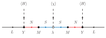
The inverse seesaw mechanism has several appealing features. First of all, we note that the resulting neutrino mass formula turns out to be proportional to the small $\mu$-parameter. This allows one to obtain light neutrino masses of the order of $0.1$ eV with TeV-scale seesaw mediators and $\mathcal{O}(1)$ Yukawa couplings, hence leading to a much richer phenomenology compared to the usual high-scale seesaw scenarios. Furthermore, we note that the $\mu$-parameter is protected by the $\rm B-L$ symmetry, since the limit $\mu\to 0$ restores $\rm U(1)_{B-L}$. This makes its smallness perfectly natural in the sense of ’t Hooft. Finally, we also note that in this construction the $\rm U(1)_{B-L}$ symmetry (or equivalently $\rm U(1)_{L}$) remains anomalous and therefore cannot be gauged. In this case they must be global symmetries, and their spontaneous breaking (by $u\neq 0$) would lead to the appearance of a Goldstone boson, the majoron.

On a side note, the reader should keep in mind that from the diagram depicted in Fig. 1 alone, one cannot distinguish between the simplest scenario in which $\rm{U(1)_{B-L}}\rightarrow\mathbb{Z}_{2}$ and more involved situations with $\rm{U(1)_{B-L}}\rightarrow\mathbb{Z}_{2n}$. Note that, when neutrinos are Majorana fermions, the residual transformation of the light neutrinos will always be $\nu\sim z^{n}=-1$ where $z=e^{i\pi/n}$. The difference between $\mathbb{Z}_{2}$ and a more complicated $\mathbb{Z}_{2n}$ cannot be seen in the neutrino mass generation but will generate differences in the scalar sector. A detailed discussion between the differences of these types of models shall be found elsewhere since it would be beyond the scope of this work.

IV The simplest Dirac inverse seesaw

In this section we aim to develop the inverse seesaw model for Dirac neutrinos. However, before going into details of the model, let us switch over to the “chiral notation” first. Thus, from now on we give the same field name to fermions who will ultimately form a VL pair. The left- and right-handed fields are distinguished with a subscript $L$ or $R$. For example, the fields of Section III get renamed as $N\to N_{L}$ and $S^{c}\to N_{R}$ in the chiral notation. This notation change is done to facilate the user to easily identify the fields which will ultimately form either a Dirac or pseudo-Dirac pair. It will become especially useful when working with Dirac neutrinos.

Furthermore, as mentioned already, throughout this work we consider symmetries to be always broken spontaneously. This choice is taken because we find that the symmetry transformations of the fields before and after breaking, as well as, the nature of the residual symmetry that is left, are more transparent when the symmetry is spontaneously broken. Also, as argued before, the spontaneous version is completely general and for any model with an explicit symmetry breaking $\mu$-term, its spontaneous symmetry breaking analogue can be always constructed. It has the added advantage that in cases where the symmetry under consideration is a gauge symmetry, only the spontaneous breaking of the symmetry is allowed and hence only spontaneously broken models are mathematically consistent.

Finally, before moving on we want to reiterate that in this work we do not attempt to answer the questions:

• How and why the $\mu$-term should be small in the first place?

• How small a $\mu$-term should be considered small?

These are important questions and are left to be addressed by the creators of a given model. We are merely assuming that, to begin with, the $\mu$-term is small. Moreover, since in the limit $\mu\to 0$ the symmetry of the system is enhanced, therefore following t’Hooft’s arguments, such a small $\mu$-term will be protected against large quantum corrections and will remain small. In the spontaneous symmetry breaking versions that we consider, this means that the VEV of the scalar which leads to the $\mu$-term will be much smaller than the electroweak VEV.

Coming back to the Dirac inverse seesaw model, note that for neutrinos to be Dirac particles, some unbroken symmetry should forbid the appearance of Majorona mass terms. This symmetry can very well be the residual symmetry $\mathcal{G}^{\prime}$ left unbroken when the $\mu$-term breaks the bigger symmetry $\mathcal{G}$, see Eq. (4). Here we will take $\mathcal{G}=\rm U(1)_{B-L}$ and $\mathcal{G}^{\prime}$ can be any of its $\mathbb{Z}_{n}$; $n>2$ subgroups Hirsch:2017col . In this section we take the simplest possibility of $\mathcal{G}^{\prime}=\mathbb{Z}_{3}$.

Symmetries play an even more central role in Dirac inverse seesaw constructs. First, a symmetry is required to ensure the Dirac nature of neutrinos i.e. to forbid Majorana mass terms for them. Second, a symmetry is also necessary to forbid the tree-level term $\bar{L}\widetilde{H}\nu_{R}$, which if present would imply tiny Yukawa couplings. Third, one must resort to a symmetry breaking argument to make the smallness of the $\mu$-parameter natural. One can accomplish these tasks by using different symmetries for each task. However, as we discuss now, the $\rm U(1)_{B-L}$ symmetry and its residual $\mathbb{Z}_{3}$ subgroup are enough to play all these roles.

We are choosing here the $\rm U(1)_{B-L}$ symmetry because it can be made anomaly free by adding right-handed neutrinos with appropriate $\rm B-L$ charges. This can be especially important if we were to gauge the symmetry, as is often done. The usual solution to make $\rm U(1)_{B-L}$ anomaly free is to add three right-handed neutrinos $\nu_{R}$ with $\rm B-L$ charges $(-1,-1,-1)$. However, an exotic choice of $\rm B-L$ charges for the right-handed neutrinos can fulfill all these conditions, the so-called 445 chiral solution Montero:2007cd ; Ma:2014qra ; Ma:2015mjd . In this case, the right-handed neutrinos carry $(-4,-4,5)$ charges under $\rm U(1)_{B-L}$. Being anomaly free, the $\rm U(1)_{B-L}$ symmetry can also be gauged, leading to a richer phenomenology. Throughout this work we will mainly use this solution in all the Dirac models that we will construct. However, let us mention that this is not the only possible symmetry solution Bonilla:2018ynb but just a particularly elegant one.

Dirac Inverse Seesaw

	Fields	$\rm SU(2)_{L}\otimes U(1)_{Y}$	$\rm U(1)_{B-L}$  $\to$  $\mathbb{Z}_{3}$	Fields	$\rm SU(2)_{L}\otimes U(1)_{Y}$	$\rm U(1)_{B-L}$  $\to$  $\mathbb{Z}_{3}$
Fermions	$L_{i}$	($\mathbf{2},{-1/2}$)	$-1\,\,\to\,\,\omega^{2}$	$\nu_{R}$	($\mathbf{1},{0}$)	$(-4,-4,5)\,\,\to\,\,\omega^{2}$
	$N_{L}$	($\mathbf{1},{0}$)	$-1\,\,\to\,\,\omega^{2}$	$N_{R}$	($\mathbf{1},{0}$)	$-1\,\,\to\,\,\omega^{2}$
Scalars	$H$	($\mathbf{2},{1/2}$)	$0\,\,\to\,\,\omega^{0}$	$\chi$	($\mathbf{1},{0}$)	$3\,\,\to\,\,\omega^{0}$

Table 2: Particle content of the minimal model implementing the Dirac inverse seesaw. All quarks transform as $1/3$ ($\omega^{1}$) under $\rm U(1)_{B-L}$ ($\mathbb{Z}_{3}$), while their $\mathrm{SU(3)_{C}\otimes SU(2)_{L}\otimes U(1)_{Y}}$  charges are identical to those in the SM. Here $\omega=e^{2\pi i/3}$ is the cube root of unity with $\omega^{3}=1$. Moreover, with this choice of charges the $\rm U(1)_{B-L}$ symmetry is anomaly free.

We begin the discussion on Dirac versions of the inverse seesaw mechanism with a very minimal realization. In this simple case, the leading effective operator for neutrino masses is $\bar{L}\widetilde{H}\chi\nu_{R}$. This corresponds to the operator in Eq. (2) with $\Phi\equiv\widetilde{H}$ where $H$ is the Higgs doublet and $\sigma\equiv\chi$; $\chi$ being an $\mathrm{SU(3)_{C}\otimes SU(2)_{L}\otimes U(1)_{Y}}$  singlet. In the full ultraviolet complete theory, the particle content and symmetry transformations are shown in Tab. 2, while the relevant Lagrangian terms for the generation of neutrino masses are given by

$$\mathcal{L}_{\rm Min}=Y\,\bar{L}\widetilde{H}N_{R}\,+\,\lambda\,\bar{N}_{L}\chi\nu_{R}\,+\,M\,\bar{N}_{L}N_{R}\,+{\rm h.c.}\,.$$ (15)

The scalar acquire VEVs

$$\langle H\rangle=v\quad,\quad\langle\chi\rangle=u\,.$$ (16)

and break the electroweak and $\rm U(1)_{B-L}$ symmetries, respectively. The VEV of $\chi$ induces the small symmetry breaking $\mu$-term.

$$\mu=\lambda\,u\,.$$ (17)

Also, note that the VEV of the singlet scalar $\chi$ breaks $\rm U(1)_{B-L}$ in three units, leaving a residual $\mathbb{Z}_{3}$ symmetry under which all scalars transform trivially while all fermions (except quarks) transform as $\omega^{2}$, with $\omega=e^{2i\pi/3};\,\omega^{3}=1$ being the cube root of unity. This symmetry forbids all Majorana terms and therefore protects the Diracness of light neutrinos. The $H$ and $\chi$ VEVs also induce Dirac masses proportional to the $Y$ and $\lambda$ Yukawa couplings. These, in the Dirac basis $\left(\bar{\nu}_{L}\,\bar{N}_{L}\right)$ and $\left(\nu_{R}\,N_{R}\right)^{T}$, gives rise to the mass matrix

$$\mathcal{M}=\left(\begin{matrix}0&Y\,v\\ \mu&M\end{matrix}\right)\,$$ (18)

where, as mentioned before, $\mu=\lambda\,u$ will be naturally small as it is the $\rm U(1)_{B-L}$ symmetry breaking term.

Thanks to the residual $\mathbb{Z}_{3}$ symmetry, the neutrinos are Dirac particles whose masses in the inverse seesaw limit $M\gg Yv\gg\mu$ are given by

$$m_{\nu}=Y\,v\,\frac{\mu}{M}\,,$$ (19)

as diagramatically shown in Fig. 2.

Figure 2: Neutrino mass generation in the minimal Dirac inverse seesaw.

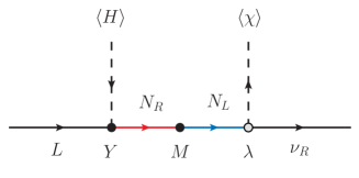
Since in the limit $\mu\to 0$ the $\rm U(1)_{B-L}$ symmetry is restored, the smallness of the $\mu$-term is protected. Its smallness will not be altered by higher order corrections, and therefore is perfectly natural. For example, if we take a small $\mu\sim 10$ eV, we can obtain $m_{\nu}\sim 0.1$ eV for $Y\sim 0.1$ and $M\sim 1$ TeV. We should also point out that the mass matrix in Eq. (18) is similar to the mass matrix one obtains in the Dirac type-I seesaw Ma:2014qra ; Ma:2015mjd ; Chulia:2016ngi ; CentellesChulia:2018gwr . However, in the type-I seesaw case, the off-diagonal terms in Eq. (18) are taken to be comparable to each other i.e. $Y\,v\approx\lambda\,u\ll M$. Thus, for Dirac neutrinos, the minimal inverse seesaw and the type-I seesaw are just two limits of the same mass matrix.

Some final comments are in order. First, since the $\rm U(1)_{B-L}$ symmetry is anomaly free, it can be a gauge symmetry. This eliminates the Goldstone boson associated to its breaking and leads to a much richer phenomenology. Note that the canonical Majorana inverse seesaw discussed in Section III is not anomaly free and hence cannot be gauged. Second, the Dirac inverse seesaw model is also relatively simple in terms of new fields added to the theory. In addition to the Standard Model   particles, we have just added the right-handed neutrinos $\nu_{R}$, a VL fermionic pair $N_{L}$ and $N_{R}$ and an extra singlet scalar $\chi$, which is needed only if the spontaneous symmetry breaking is desired.

V Generalizing the Inverse Seesaw - I : Multiplets

The canonical Majorana inverse seesaw and its Dirac analogue discussed in the previous sections are the simplest possibilities to implement the inverse seesaw mechanism. However, inverse seesaw as an idea is much more general and can be implemented in many different ways. It is the aim of this and Section VI to explore the various ways in which one can generalize it. As we show, there are several directions in which both the Dirac and Majorana inverse seesaws can be generalized. Many of these generalized models contain exotic fermions and scalars which will have very unique signatures in experiments, which we intend to explore in followup work.

In this section we restrict ourselves only to generalizing the $\rm SU(2)_{L}\times U(1)_{Y}$ multiplets that can lead to the inverse seesaw, both for Majorana and Dirac neutrinos. We will also show a few examples of each kind. We emphasize that these generalized versions may have a richer collider phenomenology than their simpler cousins.

V.1 Generalized Majorana inverse seesaw

We consider a generalization of the Majorana inverse seesaw that uses the same number of scalars and fermions as in Tab. 1 and Fig. 1, but allows for other representations under $\rm SU(2)_{L}\times U(1)_{Y}$. The Lagrangian will be formally equivalent to the one shown in III just replacing $H\rightarrow\phi$, $\chi\rightarrow\varphi$, $N\rightarrow N_{L}$ and $S^{c}\rightarrow N_{R}$, but with different multiplets of $\rm SU(2)_{L}$. There are many such generalizations possible and before we embark on their discussion, we need to streamline the notation such that the same notation can be easily applicable to Dirac as well as Majorana cases and to various possible generalizations. This generalized notation will be used throughout the rest of the paper.

• The two new type of fermions (called $N,S$ in Section III) which will ultimately form a VL pair are henceforth called by $N_{L}$ and $N_{R}$. Note that they have the same $\rm SU(2)_{L}\otimes U(1)_{Y}$ representation and $\rm B-L$ charges. Henceforth, we will denote the $\rm SU(2)_{L}$ and $\rm U(1)_{Y}$ charges of a given particle as $(\textbf{n}^{\prime},Y^{\prime})$; $\textbf{n}^{\prime}$ being the dimensionality of the $\rm SU(2)_{L}$ multiplet and $Y^{\prime}$ being its hypercharge. In this notation, the two new fermions of Section III will both have their $\rm SU(2)_{L}\otimes U(1)_{Y}$ charges given by $(1,0)$.

• We denote the scalar which couples to $L$ and $N_{R}$ as $\phi$. This scalar couples to the two fermions via the Yukawa term $\bar{L}\,\phi\,N_{R}$ and in general will transform as $(\textbf{n},Y)$ under $\rm SU(2)_{L}\otimes U(1)_{Y}$, setting $Y^{\prime}=Y-1/2$ and $\textbf{n}^{\prime}=\textbf{n}\pm 1$. Of course, n and $Y$ have to be correlated in such a way that an electrically neutral component of $\phi$ exists. For example, for $\textbf{n}=1$, only $Y=0$ is possible. For $\textbf{n}=2$, $Y=\pm 1/2$, this being the case in which $\phi$ can be identified with a SM-like Higgs i.e. either $H$ or $H^{c}$. For $\textbf{n}=3$, $Y=\pm 1,0$. For $\textbf{n}=4$, $Y=\pm 1/2,\pm 3/2$ and so on.

• The scalar whose VEV leads to the $\mu$-term will be denoted as $\varphi$. It will transform under $\rm SU(2)_{L}$ as 1, 3, 5, …2n+1 and will have a hypercharge of $1-2\,Y$. Like in the case of $\phi$, the relation between the $\rm SU(2)_{L}\otimes U(1)_{Y}$ charges of $\varphi$ have to be such that a neutral component exists in order to avoid electric charge violation.

	Fields	$\rm SU(2)_{L}\otimes U(1)_{Y}$	$\rm U(1)_{B-L}$  $\to$  $\mathbb{Z}_{2}$	Fields	$\rm SU(2)_{L}\otimes U(1)_{Y}$	$\rm U(1)_{B-L}$  $\to$  $\mathbb{Z}_{2}$
Fermions	$L_{i}$	($\mathbf{2},{-1/2}$)	$-1\,\,\to\,\,-1$
	$N_{L}$	($\mathbf{n\pm 1},{Y-1/2}$)	$-1\,\,\to\,\,-1$	$N_{R}$	($\mathbf{n\pm 1},{Y-1/2}$)	$-1\,\,\to\,\,-1$
Scalars	$H$	($\mathbf{2},{1/2})$	$0\,\,\to\,\,1$	$\phi$	($\mathbf{n},Y)$	$0\,\,\to\,\,1$
	$\varphi$	($\mathbf{1,3,5...2n+1},1-2\,Y)$	$2\,\,\to\,\,1$

Table 3: Particle content of the generalized Majorana inverse seesaw. To generate a mass for the other SM fermions, a SM-like Higgs scalar $H$ is always needed, and we have explicitly included it in the list. In some particular cases, $\phi$ can be identified with the SM-like Higgs $H$ itself i.e. $\phi\equiv H$ and two separate particles are not required. The VEV of the scalar $\varphi$ breaks the $\rm B-L$ symmetry and thus can be naturally small.

Having established our notation, let us look at the possible multiplet generalizations of the canonical inverse seesaw of Section III. Since in this section we are restricting ourselves to only multiplet generalizations, the particle content of the models remain the same. Thus, in all cases we are led to the same inverse seesaw formula in Eq. (14). However, now the fields can have more general $\rm SU(2)_{L}\otimes U(1)_{Y}$ charges, as shown in Tab. 3.

Figure 3: Generalized Majorana inverse seesaw.

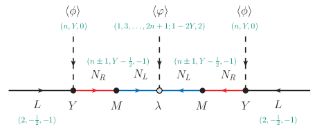
In Tab. 3, apart from the scalars $\phi$ and $\varphi$, we have also explicitly added a SM Higgs-like $\rm SU(2)_{L}$ scalar doublet $H$. In models where $\phi$ has suitable quantum numbers so as to be used for mass generation for quarks and charged leptons, a separate $H$ field is not needed. In such cases one can identify $\phi\equiv H$. The Feynman diagram for the inverse seesaw generation of neutrino masses using general multiplets is shown in Fig. 3.

Name of the model	$\phi$	$N_{L}$ and $N_{R}$	$\varphi$ ($\mu$-term)
Type I inverse seesaw - (2, 1, 0)	$(\textbf{2},1/2)=H$	(1, 0)	(1,0)
Type III inverse seesaw - (2, 1, 0)	$(\textbf{2},1/2)=H$	(3, 0)	(1,0)
Type III inverse seesaw - (2, 5, 0)	$(\textbf{2},1/2)=H$	(3, 0)	(5,0)
Type III inverse seesaw - (2, 5, 2)	(2, -1/2) = $H^{c}$	(3, -1)	(5, 2)
Type III inverse seesaw - (4, 5, 1-2Y)	(4, Y=-1/2, 3/2)	(3, Y-1/2)	(5, 1-2Y)
Type IV inverse seesaw - (3, 7, 1-2Y)	(3, Y = 0, $\pm$ 1)	$(\textbf{4},Y-1/2)$	$(\textbf{7},1-2Y)$
Type V inverse seesaw - (4, 1, 0)	(4, 1/2)	(5, 0)	(1,0)
Type V inverse seesaw - (4, 5 or 9, 0)	(4, 1/2)	(5, 0)	(5 or 9, 0)
Type V inverse seesaw - (4, 5 or 9, 1-2Y)	(4, Y=-1/2, 3/2)	(5, Y-1/2)	(5 or 9, 1-2Y)
Type V inverse seesaw - (4, 9, 4)	(4, -3/2)	(5, -2)	(9, 4)

Table 4: A few examples of the generalized inverse seesaw in the Majorana case. The nomenclature of the models is “Type X inverse seesaw - (n, m, k)” where X is the $\rm SU(2)_{L}$ multiplet of the fermion $N$, n and m are the $\rm SU(2)_{L}$ multiplets of $\phi$ and $\varphi$, respectively, and k is the hypercharge of $\varphi$. If the field $\phi$ is charged as $(\mathbf{2},-1/2)$ under $\rm SU(2)_{L}\otimes U(1)_{Y}$ then it can be identified with the SM Higgs doublet $H$ while $\varphi$ is responsible for $\rm B-L$ breaking. We are not showing the models which generate a type-II seesaw contribution. See text for detailed discussion.

Some of the simplest generalized inverse seesaw models are listed in Tab. 4. Some of the type-III models have been discussed previously in Abada:2007ux ; Gavela:2009cd ; Ibanez:2009du ; Ma:2009kh ; Eboli:2011ia ; Morisi:2012hu ; Aguilar-Saavedra:2013twa ; Law:2013gma . In Law:2013gma the first case of “Type V inverse seesaw” was also discussed. The remaining cases, to the best of our knowledge, are being discussed for first time by us. Let us now cover the simplest cases systematically.

1. For n = 1:
   The simplest case is obtained with $n=1$. In this case, the only option for the $Y$ hypercharge is $Y=0$ as any other value will lead to electric charge breaking once $\phi$ gets a VEV. Then the only option for the charges of $N_{L},N_{R}$ is $(2,-1/2)$, which are the same as for the SM lepton doublet $L$. Finally, given these charges, $\varphi$ would be forced to transform as $(\textbf{3},1)$. However, one can see that the resulting model will also induce a type II seesaw which, depending on the parameter choices, can provide the leading order contribution to the light neutrino masses, among other phenomenological issues. Thus, this choice will at best lead to a mixed inverse-typeII seesaw and not a pure inverse seesaw as desired. Hence, we reject this possibility and will not discuss it further.

2. For n = 2:
   The next case is $n=2$, where we can identify $\phi$ with either $H$ (for $Y=1/2$) or $H^{c}$ (for $Y=-1/2$). Moreover, the internal fermions $N_{R}$ and $N_{L}$ can be either singlets or triplets under $\rm SU(2)_{L}$ and will carry a hypercharge equal to $Y-1/2$ i.e. either $0$ or $-1$. Several different possibilites arise here as we discuss now:

   1. The case $Y=1/2$ with $N_{L},N_{R}\sim(\textbf{1},0)$ implies $\varphi\sim(\textbf{1},0)$. It is nothing but the canonical Majorana inverse seesaw discussed in Sec. III and studied and extensively in the literature.

   2. The case $Y=-1/2$ with $N_{L},N_{R}\sim(\textbf{1},-1)$ does not lead to any viable neutrino mass model. This is because $N_{L}$ and $N_{R}$ in this case have no electrically neutral components and hence are unsuitable to act as tree-level mediators for neutrino mass generation.

   3. Taking $N_{L}$ and $N_{R}$ to be two $\rm SU(2)_{L}$ triplets with hypercharge $0$, leads to three possibilities for $\varphi$: 1, 3 or 5 under $\rm SU(2)_{L}$. Taking $\varphi\sim\textbf{1}$ under $\rm SU(2)_{L}$ leads to the “type-III inverse seesaw” shown in Tab. 4. The option $\varphi\sim\textbf{3}$ would lead to vanishing neutrino masses since two triplets contracting to another triplet is an antisymmetric combination, which vanishes if the two fields are identical. The last option $\varphi\sim\textbf{5}$ would be the “type-III variant seesaw” shown in Tab. 4.

   4. Finally, for $N_{L},N_{R}\sim 3$ under $\rm SU(2)_{L}$ with $-1$ hypercharge, the scalar $\varphi$ can only transform as $(\textbf{5},2)$. This is a novel possibility and would represent an exotic variant of the type-III inverse seesaw. In Tab. 4 we refer to this possibility as “exotic variant I” of the type-III inverse seesaw. As opposed to the ’normal’ type-III inverse seesaw, this model will feature doubly electrically charged fermions and quadruply charged scalars.

3. For n = 3 : In the case $n=3$ we have three possibilities for $Y$: $0$ and $\pm 1$. For each value of $Y$, the fermions can transform as either doublets or quadruplets under $\rm SU(2)_{L}$, with their hypercharge values ranging from $-3/2$ to $1/2$. There are several possible cases falling under this category. These are :

   1. For $Y=1$, the fermions $N_{L}$ and $N_{R}$ will have a hypercharge of $1/2$. If they are $\rm SU(2)_{L}$ doublets, then $\varphi$ will again be an $\rm SU(2)_{L}$ triplet with hypercharge $1$. Thus, in this case, in addition to the inverse seesaw there will also be a type-II seesaw-like contribution. We therefore neglect this option. If the new fermions are quadruplets under $\rm SU(2)_{L}$, $\varphi$ will have hypercharge $-1$ and will transform as 3 or 7 under $\rm SU(2)_{L}$. However, the case $\varphi\sim(\textbf{3},-1)$ would generate a type-II seesaw contribution. We call the only remaining posibility “Type IV inverse seesaw” in Tab. 4. Note that again due to the antisymmetry of the contractions $4\times 4\rightarrow 1$ and $4\times 4\rightarrow 5$, the options of $\varphi$ transforming as 1 and 5 under $\rm SU(2)_{L}$ are both forbidden.

   2. For $Y=0$, again if the fermions are doublets then we will end up having a type-II seesaw contribution along with the inverse seesaw and as before we reject this possibility. If $N_{L}$ and $N_{R}$ are quadruplets of $\rm SU(2)_{L}$ with hypercharge $-1/2$ then again $\varphi$ will transform as 3 or 7 with hypercharge of $1$. However, as before the case $\varphi\sim(\textbf{3},1)$ would generate a type-II seesaw contribution. So again the only viable possibility is $\varphi\sim\textbf{7}$ under $\rm SU(2)_{L}$ and the resulting model is again the “Type IV inverse seesaw” given in Tab. 4.

   3. For $Y=-1$ the new fermions will have a hypercharge of $-3/2$. Thus, they cannot be doublets as in that case they will not have any electrically neutral component to act as intermediate particles for neutrino mass generation. If the fermions are quadruplets, then the only option for $\varphi$ is to transform as 7 under $\rm SU(2)_{L}$. In this case the possibility of it being a triplet will imply that $\varphi$ has no electrically neutral component and hence if it gets VEV, it would violate electric charge invariance.

   4. In summary, in all cases for $n=3$, we only have one viable possibility, namely that of the fermions transforming as quadruplets of $\rm SU(2)_{L}$ with hypercharge $Y-1/2$, while $\varphi$ will transform as $(\textbf{7},1-2Y)$.

4. For $n=4$:
   There are 4 possibilities for $Y$: $\pm 1/2$ and $\pm 3/2$. The internal fermions will be either triplets or quintuplets, while $\varphi$ will be either 1 (only for $Y=1/2$), 5 or 9 (only for the quintuplet case) under $\rm SU(2)_{L}$.

   1. The case in which $Y=1/2$ and the fermions are triplets would generate another contribution for the type-III inverse seesaw. We therefore neglect this possibility. If the fermions are quintuplets with hypercharge $0$, $\varphi$ could be either $(\textbf{1},0)$, leading to the “type-V inverse seesaw”, or a variant of it, which we call “type V variant”, with $\varphi$ transforming as either $(\textbf{5},0)$ or $(\textbf{9},0)$ as shown in Tab. 4.

   2. For $Y=-1/2$, the new fermions can be either quintuplets or triplets with hypercharge $-1$. $\varphi$ will transform as either a quintuplet, in both cases, or in the quintuplet case, as 9 with hypercharge $2$. In Tab. 4 these possibilites are listed as “type V exoctic variant I”.

   3. If $Y=3/2$ then the new fermions can be either triplets or quintuplets with hypercharge $1$. Again, $\varphi$ will transform as either a quintuplet, in both cases, or a 9 only in the quintuplet fermion case, of hypercharge $-2$. This possibility is also listed as “type V exoctic variant I” in Tab. 4.

   4. Finally, the case $Y=-3/2$ only allows for quintuplet fermions of hypercharge $-2$. The only viable option for $\varphi$ is to transform as $(\textbf{9},4)$, leading to the “type V exoctic variant II” of Tab. 4.

5. For $n>4$ :
   Higher values of $n$ are also possible. However, one can trivially generalize further to higher $n$ values and we will not discuss them explicitly.

Before ending this section, we would like to comment on the advantages of using spontaneous symmetry breaking rather than explicit breaking, when exploring the model space for any given neutrino mass generation mechanism. If one opts for explict symmetry breaking to generate the $\mu$-term, one will miss many interesting models. This is because in such case one can only consider $\mu$-terms that do not break gauge symmetries, as gauge symmetries cannot be broken explicitly. This is equivalent to restricting to only $\rm SU(2)_{L}$ singlet cases with $Y=0$ in our analysis. On the contrary, when the $\mu$-term is induced through spontaneous symmetry breaking, the field $\varphi$ whose VEV will lead to the $\mu$-term can in principle transform as any representation of the gauge groups. In cases when $\varphi$ has non-trivial $\rm SU(2)_{L}\otimes U(1)_{Y}$ transformations, its VEV will break gauge symmetry as well. However, since it is spontaneous breaking and given the hierarchy $\langle\varphi\rangle\ll v$; $v$ being the electroweak VEV, there is no issue in such a breaking. Thus, generating the $\mu$-term dynamically via spontaneous symmetry breaking reveals the full landscape of models falling under the inverse seesaw mechanism.

V.2 Generalized Dirac inverse seesaw

We now move on to the multiplet generalization of the Dirac inverse seesaw. Again, the Lagrangian of the model would be formally identical to the one in Sec. IV, but with higher $\rm SU(2)_{L}$ multiplets and replacing $H\rightarrow\phi$ and $\chi\rightarrow\varphi$. The charges under $\rm U(1)_{B-L}$ will also be identical and therefore the model would share the same appealing features. The general $\rm SU(2)_{L}\times U(1)_{Y}$ charges can be seen in Tab. 5 and diagramatically in Fig. 4.

	Fields	$\rm SU(2)_{L}\otimes U(1)_{Y}$	$\rm U(1)_{B-L}$   $\to$   $\mathbb{Z}_{3}$	Fields	$\rm SU(2)_{L}\otimes U(1)_{Y}$	$\rm U(1)_{B-L}$   $\to$   $\mathbb{Z}_{3}$
Fermions	$L_{i}$	($\mathbf{2},{-1/2}$)	$-1\,\,\to\,\,\omega^{2}$	$\nu_{R}$	($\mathbf{1},{0}$)	$(-4,-4,5)\,\to\,\omega^{2}$
	$N_{L}$	($\mathbf{n\pm 1},Y-1/2$)	$-1\,\,\to\,\,\omega^{2}$	$N_{R}$	($\mathbf{n\pm 1},Y-1/2$)	$-1\,\,\to\,\,\omega^{2}$
Scalars	$H$	($\mathbf{2},{1/2}$)	$0\,\,\to\,\,\omega^{0}$	$\varphi$	($\mathbf{n\pm 1},Y-1/2$)	$3\,\,\to\,\,\omega^{0}$
	$\phi$	($\mathbf{n},Y$)	$0\,\,\to\,\,\omega^{0}$

Table 5: Particle content of the generalized Dirac inverse seesaw. As in the Majorana case, here also $\phi$ can be identified with the SM Higgs under certain conditions. Again, $\varphi$ breaks the symmetry and generates the $\mu$-term. The particle charges under the residual $\mathbb{Z}_{3}$ symmetry are given by cube roots of unity with $\omega=e^{2\pi I/3};\,\omega^{3}=1$.

Figure 4: Generalized Dirac inverse seesaw.

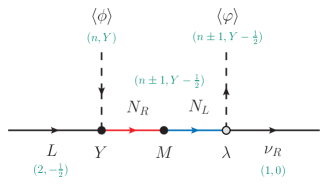
The notation and conventions here are the same as in the previous Section V.1, which generalized the inverse seesaw mechanism in the Majorana case. Here we are again using the anomaly free $(-4,-4,5)$ solution for the $\rm U(1)_{B-L}$ symmetry with the $\rm B-L$ charges of $N_{L},N_{R}$ assigned in a “vector” fashion such that the $\rm U(1)_{B-L}$ group remains anomaly free. Note that for neutrinos to remain Dirac particles, an unbroken symmetry is needed to protect their Diracness. As in Section IV, this role is again fullfiled by the unbroken residual $\mathbb{Z}_{3}$ subgroup of the $\rm U(1)_{B-L}$ symmetry, see Tab. 5.

Finally, let us list a few viable examples in Tab. 6. The general strategy to build these models is similar to that discussed at length for the Majorana case in Section V.1. We first fix the $\rm SU(2)_{L}\otimes U(1)_{Y}$ charge of the scalar $\phi$. Depending on the $\phi$ charges, the $N_{L}$ and $N_{R}$ fields can have only one option for their $\rm SU(2)_{L}\otimes U(1)_{Y}$ transformations. Finally, given the charges of both $\phi$ and the $N_{L},N_{R}$ fields, the viable options for the $\varphi$ gauge charges can be obtained. The final list of viable models for the Dirac inverse seesaw with generalized multiplets are listed in Tab. 6.

Name of the model	$N_{L}$ and $N_{R}$	$\phi$	$\varphi$ ($\mu$-term)
Standard Dirac Inverse seesaw	$(\mathbf{1},0)$	$(\mathbf{2},1/2)$	$(\mathbf{1},0)$
Type-III Dirac Inverse seesaw	$(\mathbf{3},0)$	$(\mathbf{2},1/2)$	$(\mathbf{3},0)$
Type-III Dirac Inverse seesaw variant I	$(\mathbf{3},-1)$	$(\mathbf{2},-1/2)$	$(\mathbf{3},-1)$
Type-III Dirac Inverse seesaw variant II	$(\mathbf{3},1)$	$(\mathbf{4},3/2)$	$(\mathbf{3},1)$
Exotic or Type IV Dirac inverse seesaw	$(\mathbf{4},Y-1/2)$	$(\mathbf{3},Y=0,\pm 1)$	$(\mathbf{4},Y-1/2)$
Type-V Dirac Inverse seesaw	$(\mathbf{5},0)$	$(\mathbf{4},1/2)$	$(\mathbf{5},0)$
Type-V Dirac Inverse seesaw variant I	$(\mathbf{5},1)$	$(\mathbf{4},3/2)$	$(\mathbf{5},1)$
Type-V Dirac Inverse seesaw variant II	$(\mathbf{5},-1)$	$(\mathbf{4},-1/2)$	$(\mathbf{5},-1)$
Type-V Dirac Inverse seesaw variant III	$(\mathbf{5},-2)$	$(\mathbf{4},-3/2)$	$(\mathbf{5},-2)$

Table 6: A few examples of the generalized Dirac inverse seesaw.

In Tab. 6 we have restricted outselves to $n=4$ i.e. upto the case in which $\phi$ transforms as a quadruplet under $\rm SU(2)_{L}$. Nevertheless, the generalization to higher $n>4$ is rather straightforward. Finally, as in the Majorana case, here also we have named the “type” of the model based on the $\rm SU(2)_{L}$ transformation of the $N_{L},N_{R}$ fermions. The subclass numbering is based on the $\rm SU(2)_{L}$ transformation of $\phi$ as well as the $\rm SU(2)_{L}\otimes U(1)_{Y}$ transformation of the $\varphi$ field.

VI Generalizing the inverse seesaw - II: Double inverse seesaw and beyond

We will now move into a new type of generalization of the inverse seesaw framework in which the fermionic sector of the model is extended in order to obtain double or multiple $\mu$-term supression of the neutrino mass. As before, we start with the Majorana case, showing how one can obtain a “double inverse seesaw”. We then discuss how one can generalize to triple and then multiple inverse seesaw. After that we show that the same can be done for Dirac neutrinos, explicitly working out the double and triple inverse seesaws and ending with a discussion on the Dirac multiple inverse seesaw.

VI.1 Majorana double inverse seesaw

We start the discussion with the double inverse seesaw model for Majorana neutrinos. To build a double seesaw model, consider the canonical inverse seesaw model of Sec. III and add a new fermion $S_{R}$ with $\rm B-L$ charge $0$. Moreover, let us change the charge of $\chi$ from $2$ to $1$. We keep rest of the fields and their charges identical to those in the canonical model. Therefore, the particle content and the charges of the relevant fields are given in Tab. 7.

Fields	$\rm SU(2)_{L}\otimes U(1)_{Y}$	$\rm U(1)_{B-L}$	Fields	$\rm SU(2)_{L}\otimes U(1)_{Y}$	$\rm U(1)_{B-L}$
$L$	($\mathbf{2},{-1/2}$)	$-1$	$S_{R}$	($\mathbf{1},{0}$)	$0$
$N_{L}$	($\mathbf{1},{0}$)	$-1$	$N_{R}$	($\mathbf{1},{0}$)	$-1$
$H$	($\mathbf{2},{1/2})$	$0$	$\chi$	($\mathbf{1},0)$	$1$

Table 7: Particle content of the Majorana double inverse seesaw model. In this case, the $\rm U(1)_{B-L}$ symmetry gets completely broken after $\chi$ gets a VEV.

The $\mathrm{SU(3)_{C}\otimes SU(2)_{L}\otimes U(1)_{Y}}$  and $\rm U(1)_{B-L}$ invariant Lagrangian relevant for neutrino mass generation is given by

$$\mathcal{L}_{yuk} = Y\,\bar{L}HN_{R}\,+\,M_{N}\,\bar{N}_{L}N_{R}\,+\,M_{S}\,\bar{S}_{R}S^{c}_{R}\,+\,\lambda\,\bar{N}_{L}\chi^{*}S_{R}\,+\,\lambda^{\prime}\,\bar{N}_{R}\chi S^{c}_{R}\,+\,\rm{h.c.}$$ (20)

where $Y$, $\lambda$ and $\lambda^{\prime}$ are Yukawa couplings and $M_{N}$ and $M_{S}$ are gauge invariant mass terms. As shown diagrammatically in Fig. 5, neutrino masses are generated once the scalars get VEVs, $\langle H\rangle=v$ and $\langle\chi\rangle=u$.

Figure 5: Neutrino mass generation in the double Majorana inverse seesaw.

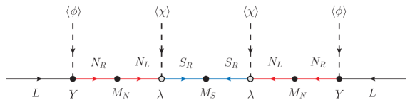
The neutral fermion mass Lagrangian after symmetry breaking is given in matrix form by

$$\mathcal{L}_{m}\,=\,\left(\begin{matrix}\bar{L}^{c}&\bar{N}_{R}&\bar{N}_{L}^{c}&\bar{S}_{R}\end{matrix}\right)\left(\begin{matrix}0&Y\,v&0&0\\ Y^{T}\,v&0&M_{N}&\mu^{\prime}\\ 0&M_{N}^{T}&0&\mu\\ 0&\mu^{{}^{\prime}T}&\mu^{T}&M_{S}\\ \end{matrix}\right)\left(\begin{matrix}L\\ N_{R}^{c}\\ N_{L}\\ S_{R}^{c}\end{matrix}\right)\,,$$ (21)

where we have defined $\mu=\lambda u$ and $\mu^{\prime}=\lambda^{\prime}u$. Curious readers will find this mass matrix a bit amusing as it does not look like an inverse seesaw mass matrix. However, this is simply because we have changed the ordering of the fields while writing the mass matrix. This is done so as to follow the sequence in which they appear in the fermionic line of Fig. 5. Since the model has symmetry breaking $\mu$-terms as well as invariant terms, the model parameters naturally follow the inverse seesaw hierarchy

$$\mu,\mu^{\prime}\ll Y\,v\ll M_{N},M_{S}\,,$$ (22)

and the light neutrino mass matrix can be obtained in seesaw approximation as

$$m_{\nu} = \left(\begin{matrix}Yv&0&0\end{matrix}\right)\left(\begin{matrix}0&M_{N}&\mu^{\prime}\\ M_{N}^{T}&0&\mu\\ \mu^{T^{\prime}}&\mu^{T}&M_{S}\\ \end{matrix}\right)^{-1}\left(\begin{matrix}Y^{T}v\\ 0\\ 0\end{matrix}\right)\,.$$ (23)

Assuming one generation for the time being, this leads to the light neutrino mass formula

$$m_{\nu}=Y^{2}\,v^{2}\,\frac{\mu^{2}}{2M_{N}\mu\mu^{\prime}-M_{N}^{2}\,M_{S}}\,\approx Y^{2}\,v^{2}\,\frac{\mu^{2}}{M_{N}^{2}\,M_{S}}.$$ (24)

One can easily see that this formula for light neutrino masses follows the same spirit as the well-known formula in the canonical Majorana inverse seesaw. However, now neutrino masses get suppressed by $\mu^{2}$ instead of $\mu$. This is the reason why we call this model double inverse seesaw.

VI.2 Majorana triple inverse seesaw and beyond

To go further along this idea, let us now add a new Weyl fermion and rearrange the $\rm B-L$ charges. We will also need to add a new symmetry-breaking scalar, see the relevant fields and charges in Tab. 8.

Fields	$\rm SU(2)_{L}\otimes U(1)_{Y}$	$\rm U(1)_{B-L}$  $\to$  $\mathbb{Z}_{2}$	Fields	$\rm SU(2)_{L}\otimes U(1)_{Y}$	$\rm U(1)_{B-L}$  $\to$  $\mathbb{Z}_{2}$
$L$	($\mathbf{2},{-1/2}$)	$-1\,\,\to\,\,-1$
$N_{L}$	($\mathbf{1},{0}$)	$-1\,\,\to\,\,-1$	$N_{R}$	($\mathbf{1},{0}$)	$-1\,\,\to\,\,-1$
$S_{L}$	($\mathbf{1},{0}$)	$a\,\,\to\,\,-1$	$S_{R}$	($\mathbf{1},{0}$)	$a\,\,\to\,\,-1$
$H$	($\mathbf{2},{1/2})$	$0\,\,\to\,\,1$
$\chi_{1}$	($\mathbf{1},0)$	$a+1\,\,\to\,\,1$	$\chi_{2}$	($\mathbf{1},0)$	$2a\,\,\to\,\,1$

Table 8: Particle content of the Majorana triple inverse seesaw model. The $\rm U(1)_{B-L}$ symmetry gets broken into the residual $\mathbb{Z}_{2}$ after $\chi_{1}$ and $\chi_{2}$ get non-zero VEVs.

To induce a triple inverse seesaw we need two different scalars carrying $\rm U(1)_{B-L}$ charges as shown in Tab. 8, with $a$ being an integer. It should be noted that $\chi_{1}$ has to be different from $\chi_{2}$ in order for the triple inverse seesaw to provide the leading order contribution. Moreover, for the same reason, the $\rm B-L$ charges of both $\chi_{1}$ and $\chi_{2}$ need to be different from $0$. The simplest solution is thus $a=2$ leading to $\chi_{1}\sim 3$ and $\chi_{2}\sim 4$. Note that $a=1$ will lead to a type-I seesaw like contribution as the leading contribution. Hence, $a\neq 1$ is required to have triple inverse seesaw as the leading contribution to neutrino masses.

Figure 6: Neutrino mass generation in the triple Majorana inverse seesaw. We note that the terms $N_{R}\,S_{L}$ and $S_{R}\,S_{R}$ cannot be avoided irrespective of the charge assignment. These terms generate $\mu^{\prime}$ terms in analogy to the standard Majorana inverse seesaw.

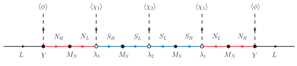
After symmetry breaking the light neutrinos become massive, as shown in the diagram of Fig. 6. The resulting neutral fermions mass Lagrangian in matrix form is given by

$$\mathcal{L}_{m}\,=\,\left(\begin{matrix}\bar{L}^{c}&\bar{N}_{R}&\bar{N}_{L}^{c}&\bar{S}_{R}&\bar{S}_{L}^{c}\end{matrix}\right)\left(\begin{matrix}0&Y\,v&0&0&0\\ Y^{T}\,v&0&M_{N}&0&\mu_{1}^{\prime}\\ 0&M^{T}_{N}&0&\mu_{1}&0\\ 0&0&\mu^{T}_{1}&\mu_{2}^{\prime}&M_{S}\\ 0&\mu^{T^{\prime}}_{1}&0&M^{T}_{S}&\mu_{2}\end{matrix}\right)\left(\begin{matrix}L\\ N_{R}^{c}\\ N_{L}\\ S_{R}^{c}\\ S_{L}\end{matrix}\right)\,+\,h.c.$$ (25)

where $\mu_{i}=\lambda_{i}u_{i}$ and $\mu^{\prime}_{i}=\lambda_{i}^{\prime}u_{i}$; $i=1,2$ with $\lambda_{i},\lambda^{\prime}_{i}$ being Yukawa couplings and $\langle\chi_{i}\rangle=u_{i}$ being the VEVs of the $\mathrm{SU(3)_{C}\otimes SU(2)_{L}\otimes U(1)_{Y}}$  singlet scalars. The model parameters naturally follow the already familiar inverse seesaw hierarchy

$$\mu_{i},\mu_{i}^{\prime}\ll Y\,v\ll M_{N},M_{S}\,.$$ (26)

Using the hierarchy of Eq. (26) in Eq. (25) we obtain the light neutrino mass matrix in seesaw approximation as

$$m_{\nu} = \left(\begin{matrix}Y\,v&0&0&0\end{matrix}\right)\left(\begin{matrix}0&M_{N}&0&\mu_{1}^{\prime}\\ M^{T}_{N}&0&\mu_{1}&0\\ 0&\mu^{T}_{1}&\mu_{2}^{\prime}&M_{S}\\ \mu^{T^{\prime}}_{1}&0&M^{T}_{S}&\mu_{2}\end{matrix}\right)^{-1}\left(\begin{matrix}Y^{T}\,v\\ 0\\ 0\\ 0\end{matrix}\right)\,.$$ (27)

Assuming one generation, one obtains the light neutrino mass formula

$$m_{\nu}=Y^{2}v^{2}\,\frac{\mu_{1}^{2}\mu_{2}}{M_{N}^{2}M_{S}^{2}-2M_{S}M_{N}\mu_{1}\mu_{1}^{\prime}+\mu_{1}^{2}\mu_{1}^{\prime 2}-M_{N}^{2}\mu_{2}\mu_{2}^{\prime}}\approx Y^{2}v^{2}\,\frac{\mu_{1}^{2}\,\mu_{2}}{M_{N}^{2}M_{S}^{2}}\,.$$ (28)

In direct analogy with the standard inverse seesaw, contributions coming from $\mu^{\prime}$ can be safely neglected. Note that here the suppression mechanism is enhanced by $\mu_{1}^{2}\mu_{2}$. Therefore, we would call this mechanism triple Majorana inverse seesaw.

Further developments into quadruple, quintuple, …, Majorana inverse seesaw mechanisms are straightforward. One indeed has to ensure that the $n$ th order inverse seesaw is the leading order contribution to neutrino masses. This can always be ensured by choosing appropriate charges for the particles transforming under the symmetry whose breaking leads to the $\mu$-terms of the model. Having ensured that, in general we find

• For $\bm{(2n-1)}$th order Inverse Seesaw:
  In this case we require “$n$ pseudo-vector pairs” of fermions and “$n$” scalars. The resulting leading neutrino masses for a $(2n-1)$th order inverse seesaw (one generation) are given by

  $$m_{\nu}\approx Y^{2}\,v^{2}\,\frac{\mu_{n}}{M_{n}^{2}}\,\prod_{i=1}^{i=n-1}\,\frac{\mu_{i}^{2}}{M_{i}^{2}}\,,$$ (29)

  where $Y$ is the Yukawa coupling involving the lepton doublet, $\mu_{i}$; $i=1,\cdots,n$ are the small symmetry breaking $\mu$-terms and $M_{i}$; $i=1,\cdots,n$ are the pseudo-Dirac masses for the pseudo-vector pairs of fermions.

• For $\bm{2n}$th order Inverse Seesaw:
  In this case we require “$n$ pseudo-vector fermion pairs”, a chiral fermion and “$n$” scalars. The resulting leading contributions to neutrino masses for a $2n$ th order inverse seesaw (one generation) are given by

  $$m_{\nu} \approx Y^{2}\,v^{2}\,\frac{1}{M_{n+1}}\,\prod_{i=1}^{i=n}\,\frac{\mu_{i}^{2}}{M_{i}^{2}}\,,$$ (30)

  where the definitions of all the couplings are the same as in the previous case.

VI.3 Dirac “Double” Inverse Seesaw

To build the double Dirac inverse seesaw, we start with the field and symmetry inventory of the minimal Dirac inverse seesaw of Section IV. To it, we add new VL fermions, $S_{L,R}$, and a new singlet scalar $\chi_{2}$. The only modification in the $\rm B-L$ charges is that we will take $(\chi_{1},\chi_{2})$ to transform as $(\chi_{1},\chi_{2})\sim(6,-9)$. Remember that in the previous example we had $\chi\sim 3$. Moreover, we take the new VL fermion to transform as $S_{L,R}\sim 5$, while the rest of the fields share their transformation properties with the previous model as shown in Tab. 9.

With the above choice of $\rm U(1)_{B-L}$ charges it is easy to check that the model is anomaly free and can be gauged if desired. Also, the $\rm B-L$ charges of the scalars are chosen in such a way that their VEVs break $\rm U(1)_{B-L}\to\mathbb{Z}_{3}$. This residual $\mathbb{Z}_{3}$ symmetry remains unbroken thus ensuring the Dirac nature of neutrinos. Note that the fields $\nu_{R}$ and $S_{R}$ share the same transformation properties, but we call them differently to follow the notational conventions of the previous and following sections.

	Fields	$\rm SU(2)_{L}\otimes U(1)_{Y}$	$\rm U(1)_{B-L}$ $\to$ $\mathbb{Z}_{3}$	Fields	$\rm SU(2)_{L}\otimes U(1)_{Y}$	$\rm U(1)_{B-L}$ $\to$ $\mathbb{Z}_{3}$
Fermions	$L_{i}$	($\mathbf{2},{-1/2}$)	$-1\,\,\to\,\,\omega^{2}$	$\nu_{R}$	($\mathbf{1},{0}$)	$(-4,-4,5)\,\,\to\,\,\omega^{2}$
	$N_{L}$	($\mathbf{1},{0}$)	$-1\,\,\to\,\,\omega^{2}$	$N_{R}$	($\mathbf{1},{0}$)	$-1\,\,\to\,\,\omega^{2}$
	$S_{L}$	($\mathbf{1},{0}$)	$5\,\,\to\,\,\omega^{2}$	$S_{R}$	($\mathbf{1},{0}$)	$5\,\,\to\,\,\omega^{2}$
Scalars	$H$	($\mathbf{2},{1/2}$)	$0\,\,\to\,\,\omega^{0}$	$\chi_{1}$	($\mathbf{1},{0}$)	$6\,\,\to\,\,\omega^{0}$
	$\chi_{2}$	($\mathbf{1},{0}$)	$-9\,\,\to\,\,\omega^{0}$

Table 9: Particle content of the Dirac analogue of the inverse seesaw. The $\rm U(1)_{B-L}$ charges of the fermions are fixed by an anomaly cancellation condition while the $\rm U(1)_{B-L}$ charges of the scalars are chosen such that the residual $\mathbb{Z}_{3}$ symmetry remains unbroken and the leading contribution to neutrino mass is induced by the double inverse seesaw.

With all these ingredients, the Lagrangian of the model relevant to neutrino mass generation is given by

$$\mathcal{L}_{\rm Dir}\,= \,Y\,\bar{L}\,\widetilde{H}\,N_{R}\,+\,\lambda_{2}\,\bar{S}_{L}\,\chi_{2}^{*}\,\nu_{R}\,+\,\lambda_{1}\,\bar{N}_{L}\,\chi_{1}^{*}\,S_{R}+\lambda^{\prime}_{1}\,\bar{S}_{L}\,\chi_{1}\,N_{R}\,$$ (31)

$$\,+\,M_{N}\,\bar{N}_{L}N_{R}\,+\,M_{S}\,\bar{S}_{L}S_{R}\,+{\rm h.c.}\,.$$ (32)

Symmetry breaking is triggered by the scalar VEVs

$$\langle H\rangle=v\quad,\quad\langle\chi_{1}\rangle=u_{1}\quad,\quad\langle\chi_{2}\rangle=u_{2}\,,$$ (33)

which lead to the following $\mu$-terms,

$$\mu_{1}=\lambda_{1}\,u_{1}\quad,\quad\mu^{\prime}_{1}=\lambda^{\prime}_{1}\,u_{1}\,\quad,\quad\mu_{2}=\lambda_{2}\,u_{2}\,.$$ (34)

After symmetry breaking, Eq. (31) leads to the mass Lagrangian in matrix form

$$\mathcal{L}_{m}=\left(\begin{matrix}\bar{\nu}_{L}&\bar{N}_{L}&\bar{S}_{L}\end{matrix}\right)\left(\begin{matrix}0&Y_{N}\,v&0\\ 0&M_{N}&\mu_{1}\\ \mu_{2}&\mu^{\prime}_{1}&M_{S}\end{matrix}\right)\left(\begin{matrix}\nu_{R}\\ N_{R}\\ S_{R}\end{matrix}\right)\,.$$ (35)

Again, the natural hierarchy among the parameters of the model is

$$\mu_{1},\mu^{\prime}_{1},\mu_{2}\ll Y\,v\ll M_{N},M_{S}\,,$$ (36)

which leads to the light neutrino mass matrix

$$m_{\nu} = \left(\begin{matrix}Y\,v&0\end{matrix}\right)\left(\begin{matrix}M_{N}&\mu_{1}\\ \mu_{1}^{\prime}&M_{S}\end{matrix}\right)^{-1}\left(\begin{matrix}0\\ \mu_{2}\end{matrix}\right)\,.$$ (37)

For one generation of light neutrinos, this is equivalent to

$$m_{\nu}=Y_{N}\,\frac{v\,\mu_{1}\,\mu_{2}}{\mu_{1}\mu^{\prime}_{1}-M_{N}M_{S}}\simeq-Y_{N}\,v\,\frac{\mu_{1}\mu_{2}}{M_{N}\,M_{S}}\,.$$ (38)

This result is illustrated in the Feynman diagram shown in Fig. 7.

Figure 7: Neutrino mass generation in the Dirac double inverse seesaw. The $\mu$-terms can be either explicit or spontaneously generated by the VEV of the scalars $\chi_{1}$ and $\chi_{2}$.

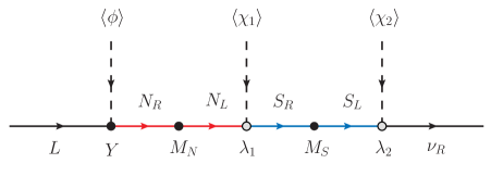
As it is clear from Eq. (38), neutrino masses in this case are suppressed by two $\mu$-terms and hence the name Dirac double inverse seesaw. Note that the effect of $\mu^{\prime}$ is subleading in the neutrino mass generation. Finally, we should remark that the spontaneous breaking of $\rm U(1)_{B-L}$ by the $u_{1}$ and $u_{2}$ VEVs leaves a residual $\mathbb{Z}_{3}$ symmetry. As in the minimal Dirac model of Section IV, here too all scalars transform trivially under this residual symmetry, while all fermions (except quarks which transform as $\omega$) transform as $\omega^{2}$. Again, this symmetry forbids all Majorana mass terms and protects the Diracness of light neutrinos.

VI.4 Dirac triple inverse seesaw and beyond

In order to build the triple Dirac inverse seesaw, we take the same field inventory as in Sec. VI.3 and add a new set of VL fermions, which we denote as $T$. Moreover, we need to add a new scalar and modify the $\rm B-L$ symmetry charges of the symmetry breaking scalars. The $\rm B-L$ anomaly free 445-solution can still be implemented, with the new fermions $S_{L,R},T_{L,R}$ getting “vector” $\rm B-L$ charges, thus preserving the anomaly free structure, see Tab. 10.

	Fields	$\rm SU(2)_{L}\otimes U(1)_{Y}$	$\rm U(1)_{B-L}$  $\to$  $\mathbb{Z}_{3}$	Fields	$\rm SU(2)_{L}\otimes U(1)_{Y}$	$\rm U(1)_{B-L}$  $\to$  $\mathbb{Z}_{3}$
Fermions	$L_{i}$	($\mathbf{2},{-1/2}$)	$-1\,\,\to\,\,\omega^{2}$	$\nu_{R}$	($\mathbf{1},{0}$)	$(-4,-4,5)\,\,\to\,\,\omega^{2}$
	$N_{L}$	($\mathbf{1},{0}$)	$-1\,\,\to\,\,\omega^{2}$	$N_{R}$	($\mathbf{1},{0}$)	$-1\,\,\to\,\,\omega^{2}$
	$S_{L}$	($\mathbf{1},{0}$)	$-4-b\,\,\to\,\,\omega^{2}$	$S_{R}$	($\mathbf{1},{0}$)	$-4-b\,\,\to\,\,\omega^{2}$
	$T_{L}$	($\mathbf{1},{0}$)	$a-1\,\,\to\,\,\omega^{2}$	$T_{R}$	($\mathbf{1},{0}$)	$a-1\,\,\to\,\,\omega^{2}$
Scalars	$H$	($\mathbf{2},{1/2}$)	$0\,\,\to\,\,\omega^{0}$	$\chi_{1}$	($\mathbf{1},{0}$)	$a\,\,\to\,\,\omega^{0}$
	$\chi_{2}$	($\mathbf{1},{0}$)	$b\,\,\to\,\,\omega^{0}$	$\chi_{3}$	($\mathbf{1},{0}$)	$-3-a-b\,\,\to\,\,\omega^{0}$

Table 10: Particle content of the triple Dirac inverse seesaw. The free charges $a$ and $b$ can only take certain values, see text for a more detailed discussion.

In this construction we must again emphasize the importance of the correct symmetry breaking pattern and the residual unbroken symmetry. If the parameters $a,b$ are chosen without care, one may generate Majorana mass terms which would in turn spoil the Dirac nature of neutrinos. For example, the choice $a=2$ would allow the presence of the mass term $\bar{N}_{L}^{c}N_{L}\chi_{2}$, which would eventually induce Majorana neutrino masses through the effective operator $\bar{L}^{c}LHH\chi_{2}$. As a general rule, the three scalars $\chi_{i}$; $i=1,2,3$ under $\rm U(1)_{B-L}$ must transform as multiples of $3$, the sum of their charges must be $3$ and none of them should have $0$ charge under the $\rm U(1)_{B-L}$ symmetry.

Figure 8: Neutrino mass generation in the Dirac triple inverse seesaw. The terms $N_{R}T_{L}$ and $T_{R}S_{L}$ cannot be avoided irrespective of the charge choices. These terms generate $\mu^{\prime}$ terms in analogy to the standard Majorana inverse seesaw, but they play a subleading role in the generation of neutrino masses.

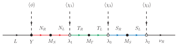
Neutrinos get massive after symmetry breaking, as shown in the diagram of Fig. 8. The neutral fermions mass Lagrangian is given by

$$\mathcal{L}_{m}=\left(\begin{matrix}\bar{\nu}_{L}&\bar{N}_{L}&\bar{S}_{L}&\bar{T}_{L}\end{matrix}\right)\left(\begin{matrix}0&Y_{N}\,v&0&0\\ 0&M_{N}&0&\mu_{2}\\ \mu_{1}&0&M_{S}&\mu_{3}^{\prime}\\ 0&\mu_{2}^{\prime}&\mu_{3}&M_{T}\end{matrix}\right)\left(\begin{matrix}\nu_{R}\\ N_{R}\\ S_{R}\\ T_{R}\end{matrix}\right)\,.$$ (39)

Here all $\mu$-terms are defined as $\mu_{i}=Y_{i}u_{i}$ and $\mu_{i}^{\prime}=Y_{i}^{\prime}u_{i}$. Again, the natural hierarchy among the parameters of the model is

$$\mu_{i},\mu_{i}^{\prime}\ll Y_{N}\,v\ll M_{N},M_{S},M_{T}\,,$$ (40)

which leads to the light neutrino mass matrix

$$m_{\nu} = \left(\begin{matrix}Y_{N}\,v&0&0\end{matrix}\right)\left(\begin{matrix}M_{N}&0&\mu_{2}\\ 0&M_{S}&\mu_{3}^{\prime}\\ \mu_{2}^{\prime}&\mu_{3}&M_{T}\end{matrix}\right)^{-1}\left(\begin{matrix}0\\ \mu_{1}\\ 0\end{matrix}\right)\,.$$ (41)

For one generation of light neutrinos this is equivalent to

$$m_{\nu}=Y_{N}\,v\,\frac{\mu_{1}\mu_{2}\mu_{3}}{M_{N}M_{S}M_{T}-M_{S}\mu_{2}\mu_{2}^{\prime}-M_{N}\mu_{3}\mu_{3}^{\prime}}\simeq Y_{N}\,v\,\frac{\mu_{1}\mu_{2}\mu_{3}}{M_{N}M_{S}M_{T}}$$ (42)

Note that again the effect of $\mu_{i}^{\prime}$ is subleading in the neutrino mass formula due to the assumed inverse seesaw hierarchy.

We finally point out that in order to induce a quadruple Dirac inverse seesaw and beyond one would just need to sequentially add a new VL fermion alongside a new scalar with a judicious choice of symmetry breaking charges for the scalars. To obtain an $n$th order Dirac inverse seesaw as the leading contribution we need to add $n$ VL fermionic pairs and $n$ scalars. Of course appropriate symmetries, with particles carrying appropriate charges under them, are required to ensure that neutrinos are Dirac particles with the leading contribution to their mass given by the $n$th order Dirac inverse seesaw as

$$m_{\nu} \approx Y\,v\,\prod_{i=1}^{i=n}\,\frac{\mu_{i}}{M_{i}}\,,$$ (43)

where as before $Y$ is the Yukawa coupling involving the lepton doublet, $\mu_{i}$; $i=1,\cdots,n$ are the small symmetry breaking $\mu$-terms and $M_{i}$; $i=1,\cdots,n$ are the masses for the vector pairs of fermions.

A combination of the generalizations shown in Sec. V and Sec. VI is straightforward and will not be developed here.

VII Summary and conclusions

To summarize, in this work we have developed the idea of inverse seesaw to encompass a whole class of mass generation mechanisms for both Majorana and Dirac neutrinos. We began by reviewing the famous canonical inverse seesaw before developing its Dirac analogue. We then showed that the idea of inverse seesaw is very general and can be implemented in a variety of ways. In particular we focused on two distinct type of extensions. In Section V we focused on developing the “multiplet” extensions of the inverse seesaw. We showed that both the canonical Majorana inverse seesaw and its Dirac analogue can be generalized by using fermions and scalars which transform as higher $\rm SU(2)_{L}$ multiplets with appropriate hypercharges. Subsequently in Section VI we discussed the “multiple $\mu$” extensions. We showed that one can generalize the idea of inverse seesaw to models where the neutrino mass is suppressed by multiple symmetry breaking $\mu$-terms. We explicitly constructed doubly and triply suppressed inverse seesaw models for both Majorana and Dirac neutrinos. This idea can in fact be generalized in a rather straightforward manner to higher order inverse seesaw models. The general mass for neutrinos in an $n$th order inverse seesaw models along with the minimal set of new particles required in such models is summarized below in Tab. 11.

Model	$m_{\nu}$ formula	New fermions	New scalars
Majorana $(2n-1)$th inverse seesaw	$Y^{2}v^{2}\frac{\mu_{n}}{M_{n}^{2}}\prod_{i=1}^{i=n-1}\frac{\mu_{i}^{2}}{M_{i}^{2}}$	$n$ VL pairs	$n$ scalars
Majorana $2n$th inverse seesaw	$Y^{2}v^{2}\frac{1}{M_{n+1}}\prod_{i=1}^{i=n}\frac{\mu_{i}^{2}}{M_{i}^{2}}$	$n$ VL pairs and a Weyl fermion	$n$ scalars
Dirac $n$th inverse seesaw	$Yv\prod_{i=1}^{i=n}\frac{\mu_{i}}{M_{i}}$	$n$ VL pairs	$n$ scalars

Table 11: The neutrino mass formula and the minimal set of fields required for an $n$th order inverse seesaw model. Note that this table is written assuming one generation of neutrinos. The mass for all three generations can be generated simply requiring multiple generations for each type of the new fermions.

It is noted that a combination of both techniques is also straightforward and hence not explicitly pursued in this work. Following the ideas above, it is possible to construct the ’multiple $\mu$’ inverse seesaw models in a framework with higher order multiplets of $\rm SU(2)_{L}\times U(1)_{Y}$.

Additionally let us emphasize the central role of the $\rm B-L$ symmetry both in the Majorana and the Dirac models. It is clear that these models need a symmetry argument in order to properly realize the inverse mechanism and, while not the only option, $\rm B-L$ represents a natural, minimal and elegant option which, in the Dirac case, can also be used to ensure the Diracness of neutrinos. Moreover, by using the anomaly free “445-solution”, we have ensured that all Dirac models are anomaly free and can therefore be gauged.

Finally the models developed here are expected to have novel and interesting phenomenological signatures, both in colliders as well as in low scale experiments like those looking for signatures of lepton flavour or lepton number breaking. We plan to systematically explore these in follow up works.

Acknoledgements

Work supported by the Spanish grants FPA2017-85216-P (MINECO/AEI/FEDER, UE), SEJI/2018/033 (Generalitat Valenciana) and FPA2017-90566-REDC (Red Consolider MultiDark), PROMETEO/2018/165 (Generalitat Valenciana). AV acknowledges financial support from MINECO through the Ramón y Cajal contract RYC2018-025795-I. The work of RS is supported by the SERB, Government of India grant under the file number SRG/2020/002303. The work of S.C.Ch. is supported by the Spanish FPI grant BES-2016-076643.

References

- (1) P. de Salas, D. Forero, C. Ternes, M. Tortola, and J. Valle, “Status of neutrino oscillations 2018: 3 hint for normal mass ordering and improved CP sensitivity,” Phys. Lett. B 782 (2018) 633–640, arXiv:1708.01186 [hep-ph].
- (2) P. de Salas, D. Forero, S. Gariazzo, P. Martínez-Miravé, O. Mena, C. Ternes, M. Tórtola, and J. Valle, “2020 Global reassessment of the neutrino oscillation picture,” arXiv:2006.11237 [hep-ph].
- (3) P. Minkowski, “ at a Rate of One Out of Muon Decays?,” Phys. Lett. B 67 (1977) 421–428.
- (4) T. Yanagida, “Horizontal gauge symmetry and masses of neutrinos,” Conf. Proc. C 7902131 (1979) 95–99.
- (5) R. N. Mohapatra and G. Senjanovic, “Neutrino Mass and Spontaneous Parity Nonconservation,” Phys. Rev. Lett. 44 (1980) 912.
- (6) M. Gell-Mann, P. Ramond, and R. Slansky, “Complex Spinors and Unified Theories,” Conf. Proc. C 790927 (1979) 315–321, arXiv:1306.4669 [hep-th].
- (7) R. N. Mohapatra and G. Senjanovic, “Neutrino Masses and Mixings in Gauge Models with Spontaneous Parity Violation,” Phys. Rev. D 23 (1981) 165.
- (8) J. Schechter and J. Valle, “Neutrino Masses in SU(2) x U(1) Theories,” Phys. Rev. D 22 (1980) 2227.
- (9) R. Foot, H. Lew, X. He, and G. C. Joshi, “Seesaw Neutrino Masses Induced by a Triplet of Leptons,” Z. Phys. C 44 (1989) 441.
- (10) E. Ma and R. Srivastava, “Dirac or inverse seesaw neutrino masses with gauge symmetry and flavor symmetry,” Phys. Lett. B 741 (2015) 217–222, arXiv:1411.5042 [hep-ph].
- (11) E. Ma, N. Pollard, R. Srivastava, and M. Zakeri, “Gauge Model with Residual Symmetry,” Phys. Lett. B 750 (2015) 135–138, arXiv:1507.03943 [hep-ph].
- (12) S. Centelles Chuliá, E. Ma, R. Srivastava, and J. W. F. Valle, “Dirac Neutrinos and Dark Matter Stability from Lepton Quarticity,” Phys. Lett. B 767 (2017) 209–213, arXiv:1606.04543 [hep-ph].
- (13) A. Zee, “A Theory of Lepton Number Violation, Neutrino Majorana Mass, and Oscillation,” Phys. Lett. B 93 (1980) 389. [Erratum: Phys.Lett.B 95, 461 (1980)].
- (14) T. Cheng and L.-F. Li, “Neutrino Masses, Mixings and Oscillations in SU(2) x U(1) Models of Electroweak Interactions,” Phys. Rev. D 22 (1980) 2860.
- (15) A. Zee, “Quantum Numbers of Majorana Neutrino Masses,” Nucl. Phys. B 264 (1986) 99–110.
- (16) K. Babu, “Model of ’Calculable’ Majorana Neutrino Masses,” Phys. Lett. B 203 (1988) 132–136.
- (17) E. Ma, “Verifiable radiative seesaw mechanism of neutrino mass and dark matter,” Phys. Rev. D 73 (2006) 077301, arXiv:hep-ph/0601225.
- (18) Y. Cai, J. Herrero-García, M. A. Schmidt, A. Vicente, and R. R. Volkas, “From the trees to the forest: a review of radiative neutrino mass models,” Front. in Phys. 5 (2017) 63, arXiv:1706.08524 [hep-ph].
- (19) C. Bonilla, E. Ma, E. Peinado, and J. W. F. Valle, “Two-loop Dirac neutrino mass and WIMP dark matter,” Phys. Lett. B 762 (2016) 214–218, arXiv:1607.03931 [hep-ph].
- (20) C. Bonilla, S. Centelles-Chuliá, R. Cepedello, E. Peinado, and R. Srivastava, “Dark matter stability and Dirac neutrinos using only Standard Model symmetries,” Phys. Rev. D 101 no. 3, (2020) 033011, arXiv:1812.01599 [hep-ph].
- (21) R. N. Mohapatra and J. W. F. Valle, “Neutrino Mass and Baryon Number Nonconservation in Superstring Models,” Phys. Rev. D34 (1986) 1642.
- (22) E. K. Akhmedov, M. Lindner, E. Schnapka, and J. Valle, “Dynamical left-right symmetry breaking,” Phys. Rev. D 53 (1996) 2752–2780, arXiv:hep-ph/9509255.
- (23) G. ’t Hooft, “Naturalness, chiral symmetry, and spontaneous chiral symmetry breaking,” NATO Sci. Ser. B 59 (1980) 135–157.
- (24) S. Centelles Chuliá, R. Srivastava, and J. W. Valle, “Seesaw roadmap to neutrino mass and dark matter,” Phys. Lett. B 781 (2018) 122–128, arXiv:1802.05722 [hep-ph].
- (25) G. Anamiati, O. Castillo-Felisola, R. M. Fonseca, J. Helo, and M. Hirsch, “High-dimensional neutrino masses,” JHEP 12 (2018) 066, arXiv:1806.07264 [hep-ph].
- (26) S. Weinberg, “Baryon and Lepton Nonconserving Processes,” Phys. Rev. Lett. 43 (1979) 1566–1570.
- (27) Y. Chikashige, R. N. Mohapatra, and R. Peccei, “Are There Real Goldstone Bosons Associated with Broken Lepton Number?,” Phys. Lett. B 98 (1981) 265–268.
- (28) J. Schechter and J. Valle, “Neutrino Decay and Spontaneous Violation of Lepton Number,” Phys. Rev. D 25 (1982) 774.
- (29) M. B. Krauss, T. Ota, W. Porod, and W. Winter, “Neutrino mass from higher than d=5 effective operators in SUSY, and its test at the LHC,” Phys. Rev. D 84 (2011) 115023, arXiv:1109.4636 [hep-ph].
- (30) S. Centelles Chuliá, R. Srivastava, and J. W. Valle, “Seesaw Dirac neutrino mass through dimension-six operators,” Phys. Rev. D 98 no. 3, (2018) 035009, arXiv:1804.03181 [hep-ph].
- (31) C.-Y. Yao and G.-J. Ding, “Systematic Study of One-Loop Dirac Neutrino Masses and Viable Dark Matter Candidates,” Phys. Rev. D 96 no. 9, (2017) 095004, arXiv:1707.09786 [hep-ph]. [Erratum: Phys.Rev.D 98, 039901 (2018)].
- (32) C.-Y. Yao and G.-J. Ding, “Systematic analysis of Dirac neutrino masses from a dimension five operator,” Phys. Rev. D 97 no. 9, (2018) 095042, arXiv:1802.05231 [hep-ph].
- (33) S. Centelles Chuliá, R. Cepedello, E. Peinado, and R. Srivastava, “Systematic classification of two loop = 4 Dirac neutrino mass models and the Diracness-dark matter stability connection,” JHEP 10 (2019) 093, arXiv:1907.08630 [hep-ph].
- (34) D. Borah and B. Karmakar, “ flavour model for Dirac neutrinos: Type I and inverse seesaw,” Phys. Lett. B 780 (2018) 461–470, arXiv:1712.06407 [hep-ph].
- (35) A. Abada and M. Lucente, “Looking for the minimal inverse seesaw realisation,” Nucl. Phys. B 885 (2014) 651–678, arXiv:1401.1507 [hep-ph].
- (36) N. Rojas, R. Srivastava, and J. W. Valle, “Scotogenic origin of the Inverse Seesaw Mechanism,” arXiv:1907.07728 [hep-ph].
- (37) F. Bazzocchi, D. Cerdeno, C. Munoz, and J. Valle, “Calculable inverse-seesaw neutrino masses in supersymmetry,” Phys. Rev. D 81 (2010) 051701, arXiv:0907.1262 [hep-ph].
- (38) F. Bazzocchi, “Minimal Dynamical Inverse See Saw,” Phys. Rev. D 83 (2011) 093009, arXiv:1011.6299 [hep-ph].
- (39) M. Hirsch, R. Srivastava, and J. W. F. Valle, “Can one ever prove that neutrinos are Dirac particles?,” Phys. Lett. B 781 (2018) 302–305, arXiv:1711.06181 [hep-ph].
- (40) J. Montero and V. Pleitez, “Gauging U(1) symmetries and the number of right-handed neutrinos,” Phys. Lett. B 675 (2009) 64–68, arXiv:0706.0473 [hep-ph].
- (41) A. Abada, C. Biggio, F. Bonnet, M. Gavela, and T. Hambye, “Low energy effects of neutrino masses,” JHEP 12 (2007) 061, arXiv:0707.4058 [hep-ph].
- (42) M. Gavela, T. Hambye, D. Hernandez, and P. Hernandez, “Minimal Flavour Seesaw Models,” JHEP 09 (2009) 038, arXiv:0906.1461 [hep-ph].
- (43) D. Ibanez, S. Morisi, and J. Valle, “Inverse tri-bimaximal type-III seesaw and lepton flavor violation,” Phys. Rev. D 80 (2009) 053015, arXiv:0907.3109 [hep-ph].
- (44) E. Ma, “Inverse Seesaw Neutrino Mass from Lepton Triplets in the U(1)(Sigma) Model,” Mod. Phys. Lett. A 24 (2009) 2491–2495, arXiv:0905.2972 [hep-ph].
- (45) O. Eboli, J. Gonzalez-Fraile, and M. Gonzalez-Garcia, “Neutrino Masses at LHC: Minimal Lepton Flavour Violation in Type-III See-saw,” JHEP 12 (2011) 009, arXiv:1108.0661 [hep-ph].
- (46) S. Morisi, E. Peinado, and A. Vicente, “Flavor origin of R-parity,” J. Phys. G 40 (2013) 085004, arXiv:1212.4145 [hep-ph].
- (47) J. Aguilar-Saavedra, P. Boavida, and F. Joaquim, “Flavored searches for type-III seesaw mechanism at the LHC,” Phys. Rev. D 88 (2013) 113008, arXiv:1308.3226 [hep-ph].
- (48) S. S. Law and K. L. McDonald, “Generalized inverse seesaw mechanisms,” Phys. Rev. D 87 no. 11, (2013) 113003, arXiv:1303.4887 [hep-ph].