When are Adaptive Strategies in Asymptotic Quantum Channel Discrimination Useful?

Abstract

Adaptiveness is a key principle in information processing including statistics and machine learning. We investigate the usefulness of an adaptive method in the framework of asymptotic binary hypothesis testing, when each hypothesis represents asymptotically many independent instances of a quantum channel, and the tests are based on using the unknown channel multiple times and observing its output at the end. Unlike the familiar setting of quantum states as hypotheses, there is a fundamental distinction between adaptive and non-adaptive strategies with respect to the channel uses, and we introduce a number of further variants of the discrimination tasks by imposing different restrictions on the test strategies.

The following results are obtained: (1) The first separation between adaptive and non-adaptive symmetric hypothesis testing exponents for quantum channels, which we derive from a general lower bound on the error probability for non-adaptive strategies; the concrete example we analyze is a pair of entanglement-breaking channels. (2) We prove that for classical-quantum channels, adaptive and non-adaptive strategies lead to the same error exponents both in the symmetric (Chernoff) and asymmetric (Hoeffding, Stein) settings. (3) We prove, in some sense generalizing the previous statement, that for general channels adaptive strategies restricted to classical feed-forward and product state channel inputs are not superior in the asymptotic limit to non-adaptive product state strategies. (4) As an application of our findings, we address the discrimination power of an arbitrary quantum channel and show that adaptive strategies with classical feedback and no quantum memory at the input do not increase the discrimination power of the channel beyond non-adaptive tensor product input strategies.

I Introduction and preliminaries

Adaptiveness is a key principle in information processing including statistics and machine learning PhysRevLett.126.190505 , which can entail great advantage over non-adaptive methods. Because of the higher complexity of adaptive methods, we thus are motivated to clarify in which situations they offer a significant improvement. Here, we address this question in the setting of binary hypothesis testing for quantum channels. Hypothesis testing is one of the most fundamental primitives both in classical and quantum information processing because a variety of other information processing problems can be cast in the framework of hypothesis testing; both direct coding theorems and converses can be reduced to it. It is expected that this analysis for adaptiveness reveals the role of adaptive methods in various types of quantum information processings. In binary hypothesis testing, the two hypotheses are usually referred to as null and alternative hypotheses and accordingly, two error probabilities are defined: type-I error due to a wrong decision in favour of the alternative hypothesis (while the truth corresponds to the null hypothesis) and type-II error due to the alternative hypothesis being rejected despite being correct. The overall objective of the hypothesis testing is to minimize the error probability in identifying the hypotheses. Depending on the significance attributed to the two types of errors, several settings can be distinguished. An historical distinction is between the symmetric and the asymmetric hypothesis testing: in symmetric hypothesis testing, the goal is to minimize both error probabilities simultaneously, while in asymmetric hypothesis testing, the goal is to minimize one type of error probability subject to a constraint on the other type of error probability.

This description of the problem presupposes that the two hypotheses correspond to objects in a probabilistic framework, in which also the possible tests (decision rules) are phrased, so as to give unambiguous meaning to the type-I and type-II error probabilities. The traditionally studied framework is that each hypothesis represents a probability distribution on a given set, and more generally a state on a given quantum system.

In the present paper, we consider the hypotheses to be described by two quantum channels, i.e. completely positive and trace preserving (cptp) maps, acting on a given quantum system, and more precisely $n\gg 1$ independent realizations of the unknown channel. It is not hard to see that both the type-I and type-II error probabilities can be made to go to $0$ exponentially fast, just as in the case of hypotheses described by quantum states, and hence the fundamental question is the characterization of the possible pairs of error exponents.

To spell out the precise questions, let us introduce a bit of notation. Throughout the paper, $A$, $B$, $C$, etc, denote quantum systems, but also their corresponding Hilbert space. We identify states $\rho$ with their density operators and use superscripts to denote the systems on which the mathematical objects are defined. The set of density matrices (positive semidefinite matrices with unit trace) on $A$ is written as $\mathcal{S}^{A}$, a subset of the trace class operators, denoted $\mathcal{T}^{A}$. When talking about tensor products of spaces, we may habitually omit the tensor sign, so $A\otimes B=AB$, etc. The capital letters $X$, $Y$, etc. denote random variables whose realizations and the alphabets will be shown by the corresponding small and calligraphic letters, respectively: $X=x\in\mathcal{X}$. All Hilbert spaces and ranges of variables may be infinite; the dimension of a Hilbert space $A$ is denoted $|A|$, as is the cardinality $|\mathcal{X}|$ of a set $\mathcal{X}$. For any positive integer $m$, we define $\vec{x}_{m}\coloneqq(x_{1},\cdots,x_{m})$. For the state $\rho\in\mathcal{S}^{AB}$ in the composite system $AB$, the partial trace over system $A$ (resp. $B$) is denoted by $\operatorname{Tr}_{A}$ (resp. $\operatorname{Tr}_{B}$). We denote the identity operator by $I$. We use $\log$ and $\ln$ to denote base $2$ and natural logarithms, respectively. Moving on to quantum channels, these are linear, completely positive and trace preserving maps $\mathcal{M}:\mathcal{S}^{A}\rightarrow\mathcal{S}^{B}$ for two quantum systems $A$ and $B$; $\mathcal{M}$ extends uniquely to a linear map from trace class operators on $A$ to those on $B$. We often denote quantum channels, by slight abuse of notation, as $\mathcal{M}:A\rightarrow B$. The ideal, or identity, channel on $A$ is denoted $\operatorname{id}_{A}$. Note furthermore that a state $\rho^{A}$ on a system $A$ can be viewed as a quantum channel $\rho:1\rightarrow A$, where $1$ denotes the canonical one-dimensional Hilbert space, isomorphic to the complex numbers $\mathbb{C}$, which interprets a state operationally consistently as a state preparation procedure.

The most general operationally justified strategy to distinguish two channels $\mathcal{M},\overline{\mathcal{M}}:A\rightarrow B$ is to prepare a state $\rho^{RA}$, apply the unknown channel to $A$ (and the identity channel $\operatorname{id}_{R}$ to $R$), and then apply a binary measurement POVM $(T,I-T)$ on $BR$, so that

$$\alpha=\operatorname{Tr}\bigl{(}(\operatorname{id}_{R}\otimes\mathcal{M})\rho\bigr{)}(I-T)\quad\text{and}\quad\beta=\operatorname{Tr}\bigl{(}(\operatorname{id}_{R}\otimes\overline{\mathcal{M}})\rho\bigr{)}T,$$

are the error probabilities of type I and type II, respectively. It is easy to see that whatever state $\rho^{AR}$ is considered as input, it can be purified to $\psi^{ARR^{\prime}}$, with a suitable Hilbert space, and the latter state can be used to get the same error probabilities. Then, once there is a pure state, one only needs a subspace of $R\otimes R^{\prime}$ of dimension $|A|$, namely the support of $\psi^{RR^{\prime}}$, which by the Schmidt decomposition is at most $|A|$-dimensional. Therefore, the state $\rho$ is without loss of generality pure and that hence $R$ has dimension at most that of $A$. The strategy is entirely described by the pair $\bigl{(}\rho,(T,I-T)\bigr{)}$ consisting of the initial state and the final measurement, and we denote it $\mathcal{T}$. Consequently, the above error probabilities are more precisely denoted $\alpha(\mathcal{M}\|\overline{\mathcal{M}}|\mathcal{T})$ and $\beta(\mathcal{M}\|\overline{\mathcal{M}}|\mathcal{T})$, respectively.

Figure 1: The most general adaptive strategy for discrimination of qq-channels, from the class $\mathbb{A}_{n}$. After the $m$-th use of the unknown channel (denoted ‘$?$’), the output system $B_{m}$ as well as the state on the memory, i.e. the reference system $R_{m}$, is processed by the cptp map $\mathcal{F}_{m}$, resulting in $\rho_{m+1}^{R_{m+1}A_{m+1}}$; this continues as long as $m<n$. After the $n$-th use of the channel, the state $\omega^{R_{n}B_{n}}_{n}$ is measured by a two-outcome POVM. Two variants of this strategy include restricting feed-forward information to be only classical, and additionally only allowing products state inputs; these variants are denoted by $\mathbb{A}_{n}^{c}$ and $\mathbb{A}_{n}^{c,0}$, respectively.

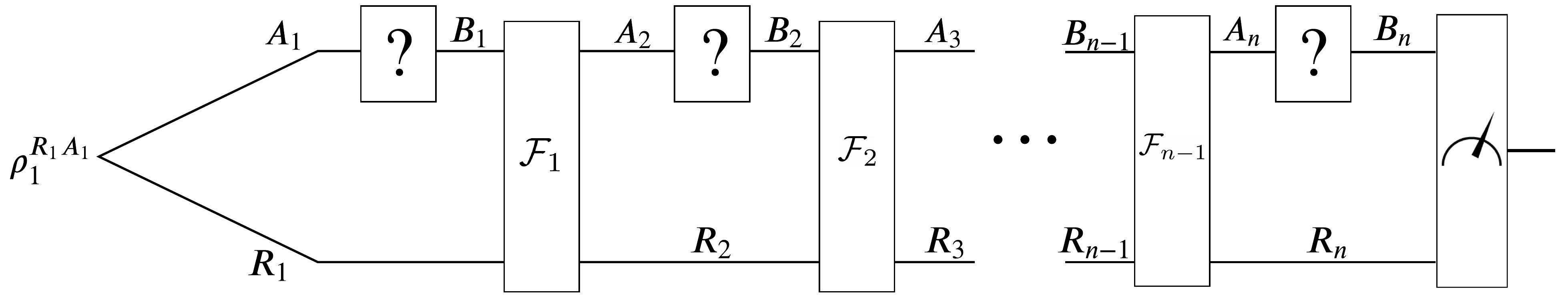
These strategies use the unknown channel exactly once; to use it $n>1$ times, one could simply consider that $\mathcal{M}^{\otimes n}$ and $\overline{\mathcal{M}}^{\otimes n}$ are quantum channels themselves and apply the above recipe. While for states this indeed leads to the most general possible discrimination strategy, for general channels other, more elaborate procedures are possible. The most general strategy we shall consider in this paper is the adaptive strategy, applying the $n$ channel instances sequentially, using quantum memory and quantum feed-forward, and a measurement at the end. This is called, variously, an adaptive strategy, a memory channel or a comb in the literature. It is defined as follows KretschmannWerner ; watrous:comb ; chiribella:memory ; chiribella:superchannel ; chiribella:comb ; 5165184 .

Definition 1.

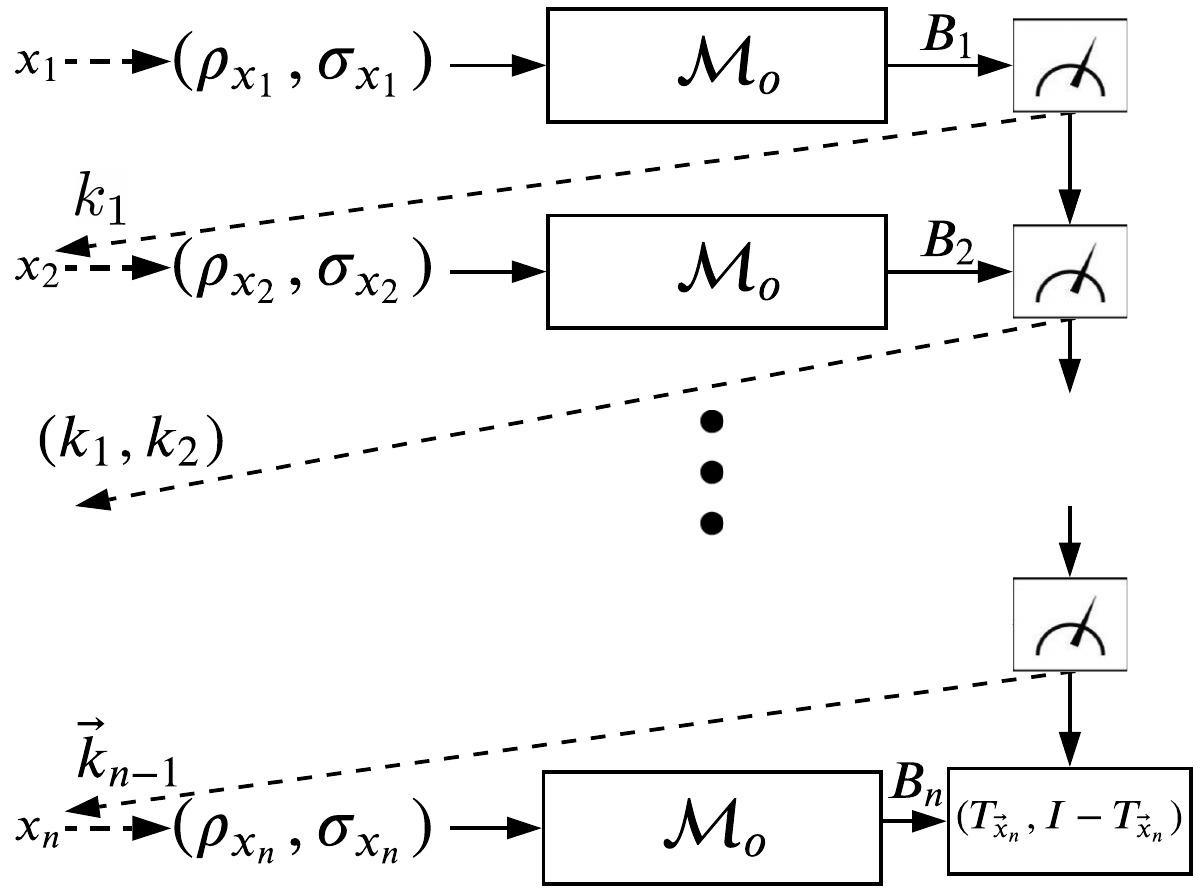
A general adaptive strategy $\mathcal{T}_{n}$ is given by an $(n+1)$-tuple $\bigl{(}\rho_{1}^{R_{1}A_{1}},\mathcal{F}_{1},\ldots,\mathcal{F}_{n-1},(T,I-T)\bigr{)}$, consisting of an auxiliary system $R_{1}$ and a state $\rho_{1}$ on $R_{1}A_{1}$, quantum channels $\mathcal{F}_{m}:R_{m}B_{m}\rightarrow R_{m+1}A_{m+1}$ and a binary POVM $(T,I-T)$ on $R_{n}B_{n}$. It encodes the following procedure (see Fig. 1): in the $m$-th round ($1\leq m\leq n$), apply the unknown channel $\Xi\in\{\mathcal{M},\overline{\mathcal{M}}\}$ to $\rho_{m}=\rho_{m}^{R_{m}A_{m}}$, obtaining

$$\omega_{m}^{R_{m}B_{m}}=\omega_{m}^{R_{m}B_{m}}(\Xi)=(\operatorname{id}_{R_{t}}\otimes\Xi)\rho_{m}^{R_{m}A_{m}}.$$

Then, as long as $m<n$, use $\mathcal{F}_{m}$ to prepare the state for the next channel use:

$$\rho_{m+1}^{R_{m+1}A_{m+1}}=\mathcal{F}_{m}(\omega_{m}^{R_{m}B_{m}}).$$

When $m=n$, measure the state $\omega_{n}^{R_{n}B_{n}}$ with $(T,I-T)$, where the first outcome corresponds to declaring the unknown channel to be $\mathcal{M}$, the second $\overline{\mathcal{M}}$. Thus, the $n$-copy error probabilities of type I and type II are given by

$$\alpha_{n}(\mathcal{M}\|\overline{\mathcal{M}}|\mathcal{T}_{n}) :=\operatorname{Tr}\bigl{(}\omega_{n}^{R_{n}B_{n}}(\mathcal{M})\bigr{)}(I-T),$$

$$\beta_{n}(\mathcal{M}\|\overline{\mathcal{M}}|\mathcal{T}_{n}) :=\operatorname{Tr}\bigl{(}\omega_{n}^{R_{n}B_{n}}(\overline{\mathcal{M}})\bigr{)}T,$$

respectively. $\square$

As in the case of a single use of the channel, one can without loss of generality (w.l.o.g.) simplify the strategy, by purifying the initial state $\rho_{1}$, hence $|R_{1}|\leq|A|$, and for each $m>1$ going to the Stinespring isometric extension of the cptp map $\operatorname{Tr}_{R_{m+1}}\circ\mathcal{F}_{m}:R_{m}B_{m}\rightarrow A_{m+1}$ that prepares the next channel input (and which by the uniqueness of the Stinespring extension is an extension of the given map $\mathcal{F}_{m}$). This requires a system $R_{m+1}$ with dimension no more than $|R_{m+1}|\leq|R_{m}||A||B|$, cf. KretschmannWerner . This allows to efficiently parametrize all strategies in the case that $A$ and $B$ are finite dimensional. An equivalent description is in terms of so-called causal channels KretschmannWerner , which are ruled by a generalization of the Choi isomorphism. This turns many optimizations over adaptive strategies into semidefinite programs (SDP) KretschmannWerner ; chiribella:comb ; Watrous:SDP ; Gutoski:diamond , which is relevant for practical calculations. See Pira:survey ; KW20 for recent comprehensive surveys of the concept of strategy and its history.

Figure 2: The most general parallel strategy for discrimination of qq-channels, from the class $\mathbb{P}_{n}$. An $(n+1)$-partite state $\rho$ on $RA_{1}\ldots A_{n}$ is prepared and each system $A_{i}$ is fed into a separate channel input; the final measurement is performed with a two-outcome POVM on $RB_{1}\ldots B_{n}$. If we do not allow input states to be entangled among different $A$-systems or with the reference system $R$, the strategy falls into the class $\mathbb{P}_{n}^{0}$.

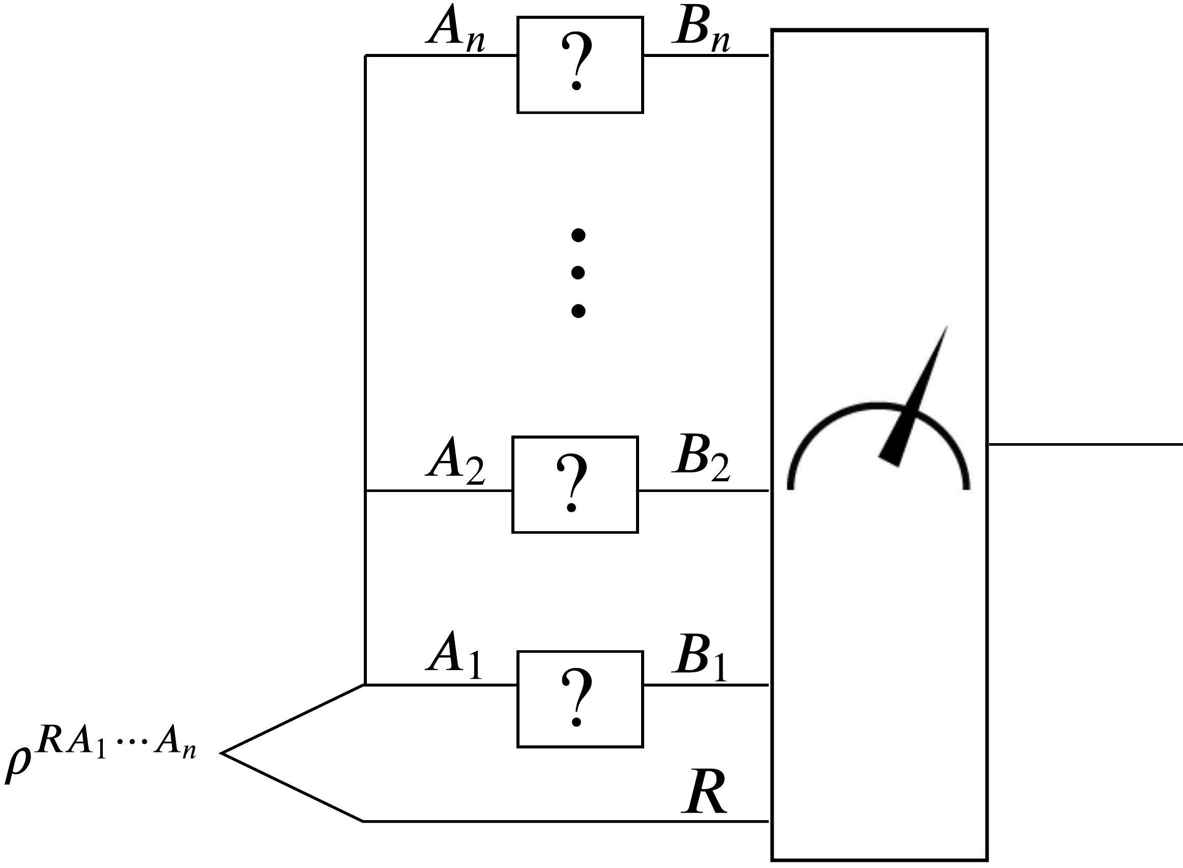
The set of all adaptive strategies of $n$ sequential channel uses is denoted $\mathbb{A}_{n}$. It quite evidently includes the $n$ parallel uses described at the beginning, when a single-use strategy is applied to the channel $C^{\otimes n}$; the set of these non-adaptive or parallel strategies is denoted $\mathbb{P}_{n}$. Among those again, we can distinguish the subclass of parallel strategies without quantum memory, meaning that $R=1$ is trivial and that the input state $\rho^{A^{n}}$ at the input system $A^{n}=A_{1}\ldots A_{n}$ is a product state, $\rho^{A^{n}}=\rho_{1}^{A_{1}}\otimes\cdots\otimes\rho_{n}^{A_{n}}$; this set is denoted $\mathbb{P}^{0}_{n}$. Other restricted sets of strategies we are considering in the present paper are that of adaptive strategies with classical feed-forward, denoted $\mathbb{A}^{c}_{n}$, and with classical feed-forward and no quantum memory at the input, denoted $\mathbb{A}^{c,0}_{n}$, as well as no quantum memory at the input but quantum feed-forward, denoted $\mathbb{A}^{0}_{n}$. They are defined formally in Section VI.

The various classes considered obey the following inclusions that are evident from the definitions. Note that all of them are strict:

$$\mathbb{A}_{n}\quad \supset \quad\mathbb{A}_{n}^{c\phantom{,0}}\quad \!\supset \quad\mathbb{P}_{n}$$

$$\cup\quad\ \cup\qquad \cup\$$ (1)

$$\mathbb{A}_{n}^{0}\quad \supset \quad\mathbb{A}_{n}^{c,0}\quad \supset \!\quad\mathbb{P}_{n}^{0}$$

In Table 3 we show a summary of the different classes and their notation, and where they are discussed.

Name	Defined	Mathematical elements	Description	Discussed
$\mathbb{A}_{n}$	Def. 1, Fig. 1	state $\rho_{1}^{R_{1}A_{1}}$, channels $\mathcal{F}_{m}:R_{m}B_{m}\rightarrow R_{m+1}A_{m+1}$, POVM $(T,I-T)$	Most general adaptive strategy of $n$ channel uses	Sec. III, VI.1, VII.2
$\mathbb{P}_{n}$	Def. 1, Fig. 2	state $\rho^{RA^{n}}$, POVM $(T,I-T)$	Most general non-adaptive (parallel) strategy allowing quantum memory at the input	Sec. III
$\mathbb{P}_{n}^{0}$	Def. 1, Fig. 2	state $\rho_{1}^{A_{1}}\otimes\cdots\otimes\rho_{n}^{A_{n}}$, POVM $(T,I-T)$	Non-adaptive (parallel) strategy without quantum memory at the input	Sec. VI.1, VI.2, VII.2
$\mathbb{A}_{n}^{c}$	Def. 19	state $\rho_{1}^{R_{1}A_{1}}$, instruments $\{\mathcal{F}_{\vec{k}_{m}}\!:\!B_{m}C_{m}\!\to\!C_{m+1}\}_{\vec{k}_{m}}$, cptp $\mathcal{P}_{\vec{k}_{m}}\!:\!R_{m}\!\to\!R_{m+1}A_{m+1}$, POVM $(T,I-T)$	Adaptive strategy of $n$ channel uses with classical feed-forward, but otherwise arbitrary quantum memory at the input	Sec. VI.3
$\mathbb{A}_{n}^{c,0}$	Def. 19, Fig. 5	states $\rho_{x_{m}}^{A_{m}}$, instruments $\{\mathcal{F}_{\vec{k}_{m}}\!:\!B_{m}C_{m}\!\to\!C_{m+1}\}_{\vec{k}_{m}}$, $q(x_{m}|\vec{x}_{m-1},\vec{k}_{m-1})$, POVM $(T,I-T)$	Adaptive strategy of $n$ channel uses with classical feed-forward, and without quantum memory at the input	Sec. VI.2, VI.3,
$\mathbb{A}_{n}^{0}$	Def. 1, Rem. 20	state $\rho_{1}^{R_{1}A_{1}}$, channels $\mathcal{F}_{m}:B_{m}C_{m}\rightarrow A_{m+1}C_{m+1}$, POVM $(T,I-T)$	Adaptive strategy of $n$ channel uses without quantum memory at the input, but otherwise arbitrary quantum feed-forward	Sec. VI.3

Figure 3: The different classes of adaptive strategies considered in the present paper, how they are denoted, where they are defined and which mathematical elements have to specified to identify a strategy from each class. In the last column we point to the sections of the paper containing results on the respective classes.

For a given class $\mathbb{S}_{n}\subset\mathbb{A}_{n}$ of adaptive strategies for any number $n$ of channel uses, the fundamental problem is now to characterize the possible pairs of error exponents for two channels $\mathcal{M}$ and $\overline{\mathcal{M}}$:

$$\mathfrak{E}(\mathcal{M}\|\mathcal{N}|\mathbb{S})$$

$$\coloneqq\left\{(r,s):\exists\mathcal{T}_{n}\in\mathbb{S}_{n}\ 0\leq r\leq\liminf_{n\rightarrow\infty}-\frac{1}{n}\log\beta_{n}(\mathcal{M}\|\overline{\mathcal{M}}|\mathcal{T}_{n}),\,0\leq s\leq\liminf_{n\rightarrow\infty}-\frac{1}{n}\log\alpha_{n}(\mathcal{M}\|\overline{\mathcal{M}}|\mathcal{T}_{n})\right\}.$$ (2)

In particular, we are interested, for each $s\geq 0$, in the largest $r$ such that $(r,s)\in\mathfrak{E}(\mathcal{M}\|\overline{\mathcal{M}}|\mathbb{S})$. To this end, we define the error rate tradeoff

$$B_{e}^{\mathbb{S}}(r|\mathcal{M}\|\overline{\mathcal{M}}):=\sup\left\{s\left|\begin{array}[]{l}\exists\mathcal{T}_{n}\in\mathbb{S}_{n}\ r\leq\liminf_{n\rightarrow\infty}-\frac{1}{n}\log\beta_{n}(\mathcal{M}\|\overline{\mathcal{M}}|\mathcal{T}_{n}),\\ s\leq\liminf_{n\rightarrow\infty}-\frac{1}{n}\log\alpha_{n}(\mathcal{M}\|\overline{\mathcal{M}}|\mathcal{T}_{n}),\end{array}\right.\right\}$$ (5)

as well as the closely related function

$$C^{\mathbb{S}}(a,b|\mathcal{M}\|\overline{\mathcal{M}}):=\inf_{\mathcal{T}_{n}\in\mathbb{S}_{n}}\liminf_{n\rightarrow\infty}-\frac{1}{n}\log\left(2^{na}\alpha_{n}(\mathcal{M}\|\overline{\mathcal{M}}|\mathcal{T}_{n})+2^{nb}\beta_{n}(\mathcal{M}\|\overline{\mathcal{M}}|\mathcal{T}_{n})\right).$$ (6)

Note that $\mathfrak{E}(\mathcal{M}\|\overline{\mathcal{M}}|\mathbb{S})$ is a closed set by definition, and for most ‘natural’ restrictions $\mathbb{S}$, it is also convex. In the latter case, the graph of $B_{e}^{\mathbb{S}}(r|\mathcal{M}\|\overline{\mathcal{M}})$ traces the upper boundary of $\mathfrak{E}(\mathcal{M}\|\overline{\mathcal{M}}|\mathbb{S})$, and it can be reconstructed from $C^{\mathbb{S}}(a,b|\mathcal{M}\|\overline{\mathcal{M}})$ by a Legendre transform.

Historically, two extreme regimes are of special interest: the maximally asymmetric error exponent,

$$\max r\text{ s.t. }\exists s\ (r,s)\in\mathfrak{E}(\mathcal{M}\|\overline{\mathcal{M}}|\mathbb{S})=\max r\text{ s.t. }(r,0)\in\mathfrak{E}(\mathcal{M}\|\overline{\mathcal{M}}|\mathbb{S}),$$

together with the opposite one of maximization of $s$, which are known as Stein’s exponents, and the symmetric error exponent

$$\begin{split}C^{\mathbb{S}}(\mathcal{M},\overline{\mathcal{M}})&=\max r\text{ s.t. }(r,r)\in\mathfrak{E}(\mathcal{M}\|\overline{\mathcal{M}}|\mathbb{S})\\ &=C^{\mathbb{S}}(0,0|\mathcal{M}\|\overline{\mathcal{M}}),\end{split}$$

which is generally known as Chernoff exponent or Chernoff bound.

In the present paper, we assume that all Hilbert spaces of interest are separable, i.e. they are spanned by countable bases, and we are primarily occupied with the performance of adaptive strategies. Naturally, the first question in this search would be to investigate the existence of quantum channels for which some class $\mathbb{S}_{n}\subset\mathbb{A}_{n}$ outperforms the parallel strategy when $n\rightarrow\infty$; in other words, if there exists a separation between adaptive and non-adaptive strategies. We study this question in general, and in particular when the channels are entanglement-breaking of the following form:

$$\mathcal{M}(\xi)={{\sum_{x}}}(\operatorname{Tr}E_{x}\xi)\rho_{x},\quad\overline{\mathcal{M}}(\xi)={{\sum_{x}}}(\operatorname{Tr}E_{x}^{\prime}\xi)\sigma_{x},$$ (7)

where $\{E_{x}\}$ and $\{E_{x}^{\prime}\}$ are PVMs and $\rho_{x},\sigma_{x}$ are states on the output system. We show that when these two PVMs are the same, $E_{x}=E_{x}^{\prime}$, then the largest class $\mathbb{A}_{n}$ cannot outperform the parallel strategy as $n\rightarrow\infty$. When the two PVMs are different, we find two examples such that the largest class $\mathbb{A}_{n}$ outperforms the parallel strategies as $n\rightarrow\infty$. For a general pair of qq-channels we focus on the class $\mathbb{A}^{c,0}_{n}$ of strategies without quantum memory at the sender’s side and with adaptive strategies that only allow for classical discrete feed-forward. We show that the class $\mathbb{A}^{c,0}_{n}$ cannot outperform the parallel strategies when $n\rightarrow\infty$. These findings are then applied to the discrimination power of a quantum channel, which quantifies how well two given states in $A^{\otimes n}$ can be discriminated after passing through a quantum channel, and whether adaptive strategies can be beneficial. To this end, we focus on a particular class of channels, namely classical-quantum channels (cq-channels) and investigate if the most general strategy offers any benefit over the most weak strategy $\mathbb{P}_{n}^{0}$. This study takes an essential role in the above problems.

The rest of the paper is organized as follows. In the following Section II we review some of the background history of hypothesis testing and previous work, this should also motives the problems we solve. In Section III we show two examples of qq-channels, of the form (7), that have the first asymptotic separation between adaptive and non-adaptive strategies via proving a lower bound on the Chernoff error for non-adaptive strategies and analyzing an example where adaptive strategies achieve error zero even with two copies of the channels. Section IV prepares notions for quantum measurements. Section V contains our analysis of cq-channel discrimination with discrete feedback variables, where we start by describing the most general adaptive strategy in this case, and mathematically define the specific quantities that we address. In Section VI, we study the discrimination of quantum channels when restricting to a subclass of $\mathbb{A}_{n}$ allowing only strategies with classical feed-forward and without quantum memory at the input. In Section VII we apply our results to the discrimination power of an arbitrary quantum channel. We conclude in Section VIII.

II History and previous work

In classical information theory, discriminating two distributions has been studied by many researchers; Stein, Chernoff chernoff1952 , Hoeffding hoeffding1965 and Han-Kobayashi 42188 formulated asymptotic hypothesis testing of two distributions as optimization problems and subsequently found optimum expressions. As generalizations of these settings to quantum realm, discrimination of two quantum states has been studied extensively in quantum information theory, albeit the complications stemming from the noncommutativity of quantum mechanics appear in the most visible way among these problems. The direct part and weak converse of the quantum extension of Stein’s lemma were proven by Hiai and Petz Hiai-Petz ; the proof combines the classical case of Stein’s lemma and the fact that for a properly chosen measurement, the classical relative entropy of the measurement outcome approaches the quantum relative entropy of the initial states. Subsequently, Ogawa and Nagaoka 887855 proved the strong converse of quantum Stein’s lemma, that is, they showed that if the error exponent of type II goes to zero exponentially fast at a rate higher than the relative entropy registered between the states, the probability of correctly identifying the null hypothesis decays to zero with a certain speed, where they found the exact expression. The Chernoff bound was settled by Nussbaum and Szkoła nussbaum2009 and Audenaert et al. Audenaert_2007 , where the former proved the converse and the latter showed its attainability (see Hayashi:book for earlier significant progress). Concerning the quantum extension of the Hoeffding bound, in 1302320 a lower bound was proved suggesting the existence of a tighter lower bound. Later, Hayashi_2007 proved the suggested tighter lower bound and subsequently, Nagaoka nagaoka2006converse showed the optimality of the above quantum Hoeffding lower bound.

Discrimination of two (quantum) channels appears as a natural extension of the state discrimination problem. However, despite inherent mathematical links between the channel and state discrimination problems, due to the additional degrees of freedom introduced by the adaptive strategies, discrimination of channels is more complicated. Many papers have been dedicated to study the potential advantages of adaptive strategies over non-adaptive strategies in channel discrimination, such as PhysRevA.81.032339 ; KPP:POVM .

The seminal classical work 5165184 showed that in the asymptotic regime, the exponential error rate for classical channel discrimination cannot be improved by adaptive strategies for any of the symmetric or asymmetric settings. For the classical channels $W:x\rightarrow W_{x}$ and $\overline{W}:x\rightarrow\overline{W}_{x}$ with common input ($\mathcal{X}$) and output ($\mathcal{Y}$) alphabets, and output distributions $\{W_{x}\}_{x\in\mathcal{X}}$ and $\{\overline{W}_{x}\}_{x\in\mathcal{X}}$, respectively, Ref. (5165184, , Thm. 1) proved the strong converse

$$B_{e}^{\mathbb{A}}(r|W\|\overline{W})=0\quad\text{if}\quad r>D(W\|\overline{W}):=\sup_{x}D(W_{x}\|\overline{W}_{x}).$$ (8)

Here, $D(W_{x}\|\overline{W}_{x})\coloneqq\sum_{y\in\mathcal{Y}}W_{x}(y)\log\frac{W_{x}(y)}{\overline{W}_{x}(y)}$ is the relative entropy. For $0\leq r\leq D(W\|\overline{W})$, Ref. (5165184, , Thm. 2) showed that

$$B_{e}^{\mathbb{A}}(r|W\|\overline{W})=B_{e}^{\mathbb{P}^{0}}(r|W\|\overline{W})=\sup_{x}\sup_{0\leq\alpha\leq 1}\frac{\alpha-1}{\alpha}\big{(}r-D_{\alpha}(W_{x}\|\overline{W}_{x})\big{)},$$ (9)

where $D_{\alpha}(W_{x}\|\overline{W}_{x})\coloneqq\frac{1}{\alpha-1}\log\sum_{y\in\mathcal{Y}}W_{x}(y)^{\alpha}\overline{W}_{x}(y)^{1-\alpha}$ is the Rényi relative entropy. Moreover, from the relation between the Hoeffding and Chernoff exponents

$$C^{\mathbb{S}}(W,\overline{W})=\sup_{r}\left\{r|B_{e}^{\mathbb{S}}(r|\mathcal{N}\|\overline{\mathcal{N}})\geq r\right\},$$

it was shown in (5165184, , Cor. 2) that

$$C^{\mathbb{A}}(W,\overline{W})=C^{\mathbb{P}^{0}}(W,\overline{W})=\sup_{x}\sup_{0\leq\alpha\leq 1}(1-\alpha)D_{\alpha}(W_{x}\|\overline{W}_{x}).$$ (10)

Since the publication of 5165184 , significant amount of research has focused on showing the potential advantages of adaptive strategies in discrimination of quantum channels. Significant progress was reported in berta2018amortized (see also Berta-ISIT ) concerning classical-quantum (cq) channels. There are other pairs of channels, for which it could be shown that adaptive strategies do not outperform non-adaptive ones for any finite number of copies, such as pairs of von Neumann measurements Puchala:measurement ; Lewandowska-et-al:measurement and teleportation-covariant channels (which are programmed by their Choi states) PL:teleport . Let $\mathcal{N}:x\rightarrow\rho_{x}$ and $\overline{\mathcal{N}}:x\rightarrow\sigma_{x}$ be two cq-channels (these channels will be formally defined in Sec. V). One may expect the same relations as (8), (9) and (10) to hold for cq-channels, replacing the Rényi relative entropy with a quantum extension of it. For Stein’s lemma and its strong converse this was indeed shown to be the case in (berta2018amortized, , Cor. 28), namely

$$B_{e}^{\mathbb{A}}(r|\mathcal{N}\|\overline{\mathcal{N}})=0\quad\text{if}\quad r>D(\mathcal{N}\|\overline{\mathcal{N}}):=\sup_{x}D(\rho_{x}\|\sigma_{x}),$$ (11)

where $D(\rho_{x}\|\sigma_{x})\coloneqq\operatorname{Tr}\rho_{x}(\log\rho_{x}-\log\sigma_{x})$ is the quantum relative entropy. Thus, one can assume $0\leq r\leq D(\mathcal{N}\|\overline{\mathcal{N}})$ for the Hoeffding and Chernoff bounds.

A number of upper bounds for $B_{e}^{\mathbb{A}}(r|\mathcal{N}\|\overline{\mathcal{N}})$ are reported in the literature but finding a compact form meeting $B_{e}^{\mathbb{P}^{0}}(r|\mathcal{N}\|\overline{\mathcal{N}})$ has been an open problem. Two such upper bounds were reported by Wilde et al. berta2018amortized ; the first upper bound follows the similar reasoning as in the classical Hoeffding bound 5165184 , that is, considering an intermediate channel and using the strong and weak Stein’s lemma. However, unlike the classical case, this line of reasoning could not yield a tight bound. Note that besides (9), in the classical case there is another compact expression for $B_{e}^{\mathbb{A}}(r|W\|\overline{W})$

$$B_{e}^{\mathbb{A}}(r|W\|\overline{W})=\sup_{x\in\mathcal{X}}\min_{Q:D(Q\|\overline{W}_{x})\leq r}D(Q\|W_{x}).$$

The reason that the classical approach of 5165184 does not yield a tight bound in the quantum case is that (Hayashi:book, , Sec. 3.8)

$$B_{e}^{\mathbb{A}}(r|\mathcal{N}\|\overline{\mathcal{N}})\leq\max_{x\in\mathcal{X}}\min_{\tau:D(\tau\|\sigma_{x})\leq r}D(\tau\|\rho_{x}).$$

The second upper bound of Wilde et al. berta2018amortized employs the fact that cq-channels are environment-parameterized: Due to the structure of the environment-parametrized channels, any $n$-round adaptive channel discrimination protocol can be understood as a particular kind of state discrimination protocol for the environment states of each channel. This development reduces the cq-channel discrimination problem to that of state discrimination between $(\bigotimes_{x}\rho_{x})^{\otimes n}$ and $(\bigotimes_{x}\sigma_{x})^{\otimes n}$ (for finite $\mathcal{X}$). However, plugging the states into the well-known state discrimination bounds does not lead to a tight characterization.

In general quantum channel discrimination, it is known that adaptive strategies offer an advantage in the non-asymptotic regime for discrimination in the symmetric Chernoff setting PhysRevA.81.032339 ; PhysRevLett.103.210501 ; 7541701 ; cite-key . In particular, Harrow et al. PhysRevA.81.032339 demonstrated the advantage of adaptive strategies in discriminating a pair of entanglement-breaking channels that requires just two channel evaluations to distinguish them perfectly, but such that no non-adaptive strategy can give perfect distinguishability using any finite number of channel evaluations. However, it was open whether the same holds in the asymptotic setting.

This question in the asymmetric regime was recently settled by Wang and Wilde: In (PhysRevResearch.1.033169, , Thm. 3), they found an exponent in Stein’s setting for non-adaptive strategies in terms of channel max-relative entropy, also in the same paper (PhysRevResearch.1.033169, , Thm. 6), they found an exponent in Stein’s setting for the adaptive strategies in terms of amortized channel divergence, a quantity introduced in berta2018amortized to quantify the largest distinguishability between two channels. However, the fact that adaptive strategies do not offer an advantage in the setting of Stein’s lemma for quantum channels, i.e. the equality of the aforementioned exponents of Wang and Wilde, was later shown in fang2019chain via a chain rule for the quantum relative entropy proven therein.

Cooney et al. Cooney2016 proved the quantum Stein’s lemma for discriminating between an arbitrary quantum channel and a “replacer channel” that discards its input and replaces it with a fixed state. This work led to the conclusion that at least in the asymptotic regime, a non-adaptive strategy is optimal in the setting of Stein’s lemma. However, in the Hoeffding and Chernoff settings, the question of potential advantages of adaptive strategies involving replacer channels remains open.

Hirche et al. Hirche studied the maximum power of a fixed quantum detector, i.e. a POVM, in discriminating two possible states. This problem is dual to the state discrimination scenario considered so far in that, while in the state discrimination problem the state pair is fixed and optimization is over all measurements, in this problem a measurement POVM is fixed and the question is how powerful this discriminator is, and then whatever criterion considered for quantifying the power of the given detector, it should be optimized over all input states. In particular, if $n\geq 2$ uses of the detector are available, the optimization takes place over all $n$-partite entangled states and also all adaptive strategies that may help improve the performance of the measurement. The main result of Hirche states that when asymptotically many uses (i.e. $n\rightarrow\infty$) of a given detector is available, its performance does not improve by considering general input states or using an adaptive strategy in any of the symmetric or asymmetric settings described before.

III Asymptotic separation between adaptive and non-adaptive strategies

III.1 Useful proposition for asymptotic separation

In this section we exhibit an asymptotic separation between the Chernoff error exponents of discriminating between two channels by adaptive versus non-adaptive strategies. Concretely, we will show that two channels described in PhysRevA.81.032339 , and shown to be perfectly distinguishable by adaptive strategies of $n\geq 2$ copies, hence having infinite Chernoff exponent, nevertheless have a finite error exponent under non-adaptive strategies.

The separation is based on a general lower bound on non-adaptive strategies for an arbitrary pair of channels. Consider two quantum channels, i.e. cptp maps, $\mathcal{M},\overline{\mathcal{M}}:A\rightarrow B$. To fix notation, we can write their Kraus decompositions as

$$\mathcal{M}(\rho)=\sum_{i}E_{i}\rho E_{i}^{\dagger},\quad\overline{\mathcal{M}}(\rho)=\sum_{j}F_{j}\rho F_{j}^{\dagger}.$$

The most general strategy to distinguish them consists in the preparation of a, w.l.o.g. pure, state $\varphi$ on $A\otimes R$, where $R\simeq A$, send it through the unknown channel, and make a binary measurement $(T,I-T)$ on $B\otimes R$:

$$p=\operatorname{Tr}\left((\operatorname{id}_{R}\otimes\mathcal{M})\varphi\right)T,\quad q=\operatorname{Tr}\left((\operatorname{id}_{R}\otimes\overline{\mathcal{M}})\varphi\right)T,$$

and likewise $1-p$ and $1-q$ by replacing $T$ in the above formulas with $I-T$. Note that for uniform prior probabilities on the two hypotheses, the error probability in inferring the true channel from the measurement output is $\frac{1}{2}(1-|p-q|)$.

The maximum of $|p-q|$ over state preparations and measurements gives rise to the (normalized) diamond norm distance of the channels Kitaev ; AKN ; Paulsen:book ; Watrous:SDP :

$$\max_{\varphi,T}|p-q|=\frac{1}{2}\|\mathcal{M}-\overline{\mathcal{M}}\|_{\diamond},$$

which in turn quantifies the minimum discrimination error under the most general quantum strategy:

$$P_{e}=\frac{1}{2}\left(1-\frac{1}{2}\|\mathcal{M}-\overline{\mathcal{M}}\|_{\diamond}\right).$$

We are interested in the asymptotics of this error probability when the discrimination strategy has access to $n\gg 1$ many instances of the unknown channel in parallel, or in other words, in a non-adaptive way. This means effectively that the two hypotheses are the simple channels $\mathcal{M}^{\otimes n}$ and $\overline{\mathcal{M}}^{\otimes n}$, so that the error probability is

$$P_{e,\mathbb{P}}^{(n)}=\frac{1}{2}\left(1-\frac{1}{2}\left\|\mathcal{M}^{\otimes n}-\overline{\mathcal{M}}^{\otimes n}\right\|_{\diamond}\right).$$

The (non-adaptive) Chernoff exponent is then given as

$$C^{\mathbb{P}}(\mathcal{M},\overline{\mathcal{M}})=\lim_{n\rightarrow\infty}-\frac{1}{n}\log P_{e,\mathbb{P}}^{(n)},$$

the existence of the limit being guaranteed by general principles. Note that the limit can be $+\infty$, which happens in all cases where there is an $n$ such that $P_{e,\mathbb{P}}^{(n)}=0$. It is currently unknown whether this is the only case; cf. the case of the more flexible adaptive strategies, for which there is a simple criterion to determine whether there exists an $n$ such that the adaptive error probability $P_{e,\mathbb{A}}^{(n)}=0$ PhysRevLett.103.210501 , and then evidently $C^{\mathbb{A}}(\mathcal{M},\overline{\mathcal{M}})=+\infty$; conversely, we know that in all other cases, the adaptive Chernoff exponent is $C^{\mathbb{A}}(\mathcal{M},\overline{\mathcal{M}})<+\infty$ 2017arXiv170501642Y . There exist also other lower bounds on the symmetric discrimination error by adaptive strategies, for instance (PLLP:lowerbound, , Thm. 3) geared towards finite $n$.

Duan et al. 7541701 have attempted a characterization of the channel pairs such that there exists an $n$ with $P_{e,\mathbb{P}}^{(n)}=0$, and have given a simple sufficient condition for the contrary. Namely, the existing result (7541701, , Cor. 1) states that if $\operatorname{span}\{E_{i}^{\dagger}F_{j}\}$ contains a positive definite element, then for all $n$ we have $P_{e,\mathbb{P}}^{(n)}>0$. The following proposition, which makes the result of 7541701 quantitative, is the main result of this section.

Proposition 2.

Let $\alpha_{ij}\in\mathbb{C}$ be such that $\sum_{ij}|\alpha_{ij}|^{2}=1$ and $P:=\sum_{ij}\alpha_{ij}E_{i}^{\dagger}F_{j}>0$, i.e. $P$ is assumed to be positive definite. Then for all $n$,

$$P_{e,\mathbb{P}}^{(n)}\geq\frac{1}{4}\lambda_{\min}(P)^{4n},$$

where $\lambda_{\min}(A)$ denotes the smallest eigenvalue of the Hermitian operator $A$. Consequently,

$$C^{\mathbb{P}}(\mathcal{M},\overline{\mathcal{M}})\leq 4\log\|P^{-1}\|_{\infty}.$$

Proof.

We begin with a test state $\varphi$ as in the above description of the most general non-adaptive strategy for the channels $\mathcal{M}$ and $\overline{\mathcal{M}}$, so that the two output states are $\rho=(\operatorname{id}_{R}\otimes\mathcal{M})\varphi$, $\sigma=(\operatorname{id}_{R}\otimes\overline{\mathcal{M}})\varphi$. By well-known inequalities 761271 , it holds

$$\frac{1}{2}\|\rho-\sigma\|_{1}\leq\sqrt{1-F(\rho,\sigma)^{2}}\leq 1-\frac{1}{2}F(\rho,\sigma)^{2},$$

where $F(\rho,\sigma)=\|\sqrt{\rho}\sqrt{\sigma}\|_{1}$ is the fidelity. Thus, it will be enough to lower bound the fidelity between the output states of the two channels. With $\tau=\operatorname{Tr}_{R}\outerproduct{\varphi}{\varphi}$, we have:

$$\begin{split}F(\rho,\sigma)&=\|\sqrt{\rho}\sqrt{\sigma}\|_{1}\\ &\geq\operatorname{Tr}\sqrt{\rho}\sqrt{\sigma}\\ &\geq\operatorname{Tr}\rho\sigma\\ &=\sum_{ij}|\operatorname{Tr}E_{i}^{\dagger}F_{j}\tau|^{2}\\ &\geq\left|\sum_{ij}\alpha_{ij}\operatorname{Tr}E_{i}^{\dagger}F_{j}\tau\right|^{2}\\ &=|\operatorname{Tr}\tau P|^{2}.\end{split}$$

Here, the second line is by standard inequalities for the trace norm, the third is because of $\rho\leq\sqrt{\rho}$, the fourth is a formula from (7541701, , Sec. II), in the fifth we used Cauchy-Schwarz inequality and in the last line the definition of $P$. Since $\tau$, like $\varphi$, ranges over all states, we get

$$F(\rho,\sigma)^{2}\geq\lambda_{\min}(P)^{4},$$

and so

$$P_{e}\geq\frac{1}{4}\lambda_{\min}(P)^{4}.$$

We can apply the same reasoning to $\mathcal{M}^{\otimes n}$ and $\overline{\mathcal{M}}^{\otimes n}$, for which the vector $(\alpha_{ij})^{\otimes n}$ is eligible and leads to the positive definite operator $P^{\otimes n}$. Thus,

$$P_{e,\mathbb{P}}^{(n)}\geq\frac{1}{4}\lambda_{\min}\left(P^{\otimes n}\right)^{4}=\frac{1}{4}\lambda_{\min}(P)^{4n}.$$

Taking the limit and noting $\lambda_{\min}(P)^{-1}=\|P^{-1}\|_{\infty}$ concludes the proof. ∎

III.2 Two examples

Example 3.

Next we show that two channels defined by Harrow et al. PhysRevA.81.032339 yield an example of a pair with $C^{\mathbb{P}}(\mathcal{M},\overline{\mathcal{M}})<+\infty$, yet $C^{\mathbb{A}}(\mathcal{M},\overline{\mathcal{M}})=+\infty$ because indeed $P_{e,\mathbb{A}}^{(2)}=0$. In PhysRevA.81.032339 , the following two entanglement-breaking channels from $A\otimes C=\mathbb{C}^{2}\otimes\mathbb{C}^{2}$ (two qubits) to $B=\mathbb{C}^{2}$ (one qubit) are considered:

$$\mathcal{M}(\rho^{A}\otimes\gamma^{C}) =\outerproduct{0}{0}\bra{0}\gamma\ket{0}+\outerproduct{0}{0}\bra{1}\gamma\ket{1}\bra{0}\rho\ket{0}+\frac{1}{2}I\bra{1}\gamma\ket{1}\bra{1}\rho\ket{1},$$

$$\overline{\mathcal{M}}(\rho^{A}\otimes\gamma^{C}) =\outerproduct{+}{+}\bra{0}\gamma\ket{0}+\outerproduct{1}{1}\bra{1}\gamma\ket{1}\bra{+}\rho\ket{+}+\frac{1}{2}I\bra{1}\gamma\ket{1}\bra{-}\rho\ket{-},$$

extended by linearity to all states. Here, $\ket{0},\ket{1}$ are the computational basis ($Z$ eigenbasis) of the qubits, while $\ket{+},\ket{-}$ are the Hadamard basis ($X$ eigenbasis).

In words, both channels measure the qubit $C$ in the computational basis. If the outcome is ‘0’, they each prepare a pure state on $B$ (ignoring the input in $A$): $\outerproduct{0}{0}$ for $\mathcal{M}$, $\outerproduct{+}{+}$ for $\overline{\mathcal{M}}$. If the outcome is ‘1’, they each make a measurement on $A$ and prepare an output state on $B$ depending on its outcome: standard basis measurement for $\mathcal{M}$ with $\outerproduct{0}{0}$ on outcome ‘0’ and the maximally mixed state $\frac{1}{2}I$ on outcome ‘1’; Hadamard basis measurement for $\overline{\mathcal{M}}$ with $\outerproduct{1}{1}$ on outcome ‘+’ and the maximally mixed state $\frac{1}{2}I$ on outcome ‘-’. In PhysRevA.81.032339 , a simple adaptive strategy for $n=2$ uses of the channel is given that discriminates $\mathcal{M}$ and $\overline{\mathcal{M}}$ perfectly: The first instance of the channel is fed with $\outerproduct{0}{0}\otimes\outerproduct{0}{0}$, resulting in an output state $\rho_{1}$; the second instance of the channel is fed with $\outerproduct{1}{1}\otimes\rho_{1}$; the output state $\rho_{2}$ of the second instance is $\outerproduct{0}{0}$ if the unknown channel is $\mathcal{M}$, and $\outerproduct{1}{1}$ if the unknown channel is $\overline{\mathcal{M}}$, so a computational basis measurement reveals it. Note that no auxiliary system $R$ is needed, but the feed-forward nevertheless requires a qubit of quantum memory for the strategy to be implemented. In any case, this proves that $P_{e,\mathbb{A}}^{(2)}=0$. In PhysRevA.81.032339 , it is furthermore proved that for all $n\geq 1$, $P_{e,\mathbb{P}}^{(n)}>0$.

We now show that Proposition 2 is applicable to yield an exponential lower bound on the non-adaptive error probability. The Kraus operators of the two channels can be chosen as follows:

$$\mathcal{M}:E_{i}\in\Bigl{\{}\ket{0}^{B} \bra{00}^{AC}, \quad\overline{\mathcal{M}}:F_{j}\in\Bigl{\{}\ket{+}^{B} \bra{00}^{AC},$$

$$\ket{0}^{B} \bra{10}^{AC}, \ket{+}^{B} \bra{10}^{AC},$$

$$\ket{0}^{B} \bra{01}^{AC}, \ket{1}^{B} \bra{+1}^{AC},$$

$$\ket{0}^{B} \bra{11}^{AC}/\sqrt{2}, \ket{0}^{B} \bra{-1}^{AC}/\sqrt{2},$$

$$\ket{1}^{B} \bra{11}^{AC}/\sqrt{2}\Bigr{\}}, \ket{1}^{B} \bra{-1}^{AC}/\sqrt{2}\Bigr{\}}.$$

Thus, the products $E_{i}^{\dagger}F_{j}$ include the matrices

$$E_{1}^{\dagger}F_{1} =\sqrt{\frac{1}{2}}\outerproduct{00}{00},$$

$$E_{2}^{\dagger}F_{2} =\sqrt{\frac{1}{2}}\outerproduct{10}{10},$$

$$E_{5}^{\dagger}F_{3} =\sqrt{\frac{1}{2}}\outerproduct{11}{+1},$$

$$E_{5}^{\dagger}F_{5} =\frac{1}{2}\outerproduct{11}{-1},$$

$$E_{3}^{\dagger}F_{4} =\sqrt{\frac{1}{2}}\outerproduct{01}{-1},$$

from which we can form, by linear combination, the operators

$$E_{1}^{\dagger}F_{1} =\sqrt{\frac{1}{2}}\outerproduct{0}{0}\otimes\outerproduct{0}{0},$$

$$E_{2}^{\dagger}F_{2} =\sqrt{\frac{1}{2}}\outerproduct{1}{1}\otimes\outerproduct{0}{0},$$

$$\sqrt{\frac{1}{2}}E_{5}^{\dagger}F_{3}-E_{5}^{\dagger}F_{5} =\sqrt{\frac{1}{2}}\outerproduct{1}{1}\otimes\outerproduct{1}{1},$$

$$\sqrt{\frac{1}{2}}E_{3}^{\dagger}F_{4}-E_{5}^{\dagger}F_{5} =\sqrt{\frac{1}{2}}\outerproduct{-}{-}\otimes\outerproduct{1}{1},$$

whose sum is indeed positive definite, so we get an exponential lower bound on $P_{e,\mathbb{P}}^{(n)}$ and hence a finite value of $C^{\mathbb{P}}(\mathcal{M},\overline{\mathcal{M}})$. To get a concrete upper bound on $C^{\mathbb{P}}(\mathcal{M},\overline{\mathcal{M}})$ from the above method, we make the ansatz

$$\begin{split}P&=\alpha E_{1}^{\dagger}F_{1}+\alpha E_{2}^{\dagger}F_{2}+\beta\sqrt{\frac{1}{2}}E_{5}^{\dagger}F_{3}+\beta\sqrt{\frac{1}{2}}E_{3}^{\dagger}F_{4}-2\beta E_{5}^{\dagger}F_{5}\\ &=\alpha\sqrt{\frac{1}{2}}I\otimes\outerproduct{0}{0}+\beta\sqrt{\frac{1}{2}}(\outerproduct{1}{1}+\outerproduct{-}{-})\otimes\outerproduct{1}{1},\end{split}$$

where $\alpha,\beta>0$ and $2\alpha^{2}+5\beta^{2}=1$. Now $P$ is an orthogonal sum of two rank-two operators, i.e. as a $4\times 4$-matrix it has block diagonal structure with two $2\times 2$-blocks. Their minimum eigenvalues are easily calculated: they are $\alpha\sqrt{\frac{1}{2}}$ and $\beta\sqrt{2}\sin^{2}\frac{\pi}{8}$. Since $\lambda_{\min}(P)$ will be the smaller of the two, we optimize it by making the two values equal, i.e. we want $\alpha=2\beta\sin^{2}\frac{\pi}{8}$. Inserting this in the normalization condition and solving for $\beta$ yields $\beta^{2}=\left(8\sin^{4}\frac{\pi}{8}+5\right)^{-1}$, thus

$$\lambda_{\min}(P)=\sqrt{\frac{2}{8\sin^{4}\frac{\pi}{8}+5}}\sin^{2}\frac{\pi}{8}=\frac{2-\sqrt{2}}{4\sqrt{4-\sqrt{2}}}\approx 0.091,$$

where we have used the identity $\sin^{2}\frac{\pi}{8}=\frac{1}{2}(1-\sqrt{\frac{1}{2}})$. Hence we conclude

$$C^{\mathbb{P}}(\mathcal{M},\overline{\mathcal{M}})\leq 4\log\frac{4\sqrt{4-\sqrt{2}}}{2-\sqrt{2}}\approx 13.83.$$

Note that a lower bound is the Chernoff bound of the two pure output states $\outerproduct{0}{0}=\mathcal{M}(\outerproduct{00}{00})$ and $\outerproduct{+}{+}=\overline{\mathcal{M}}(\outerproduct{00}{00})$, which is $\log 2=1$, so $C^{\mathbb{P}}(\mathcal{M},\overline{\mathcal{M}})\geq 1$. It seems reasonable to conjecture that this is optimal, but we do not have at present a proof of it. $\square$

Example 4.

For later use, we briefly discuss another example due to Krawiec et al. KPP:POVM , which consists of two quantum-classical channels (qc-channels) implementing two rank-one POVMs on a qutrit $A$, and the output $Y$ is a nine-dimensional Hilbert space. They are given by vectors $\ket{x_{i}}\in A$ and $\ket{y_{i}}\in A$ ($i=1,\ldots,9$) such that $\sum_{i=1}^{9}\outerproduct{x_{i}}{x_{i}}=\sum_{j=1}^{9}\outerproduct{y_{j}}{y_{j}}=I$:

$$\mathcal{P}(\rho)=\sum_{i=1}^{9}\bra{x_{i}}\rho\ket{x_{i}}\outerproduct{i}{i},\quad\overline{\mathcal{P}}(\rho)=\sum_{j=1}^{9}\bra{y_{j}}\rho\ket{y_{j}}\outerproduct{j}{j}.$$ (12)

The Kraus operators are $E_{i}=\outerproduct{i}{x_{i}}$ and $F_{j}=\outerproduct{j}{y_{j}}$, which makes it easy to calculate $\operatorname{span}\{E_{i}^{\dagger}F_{j}\}=\operatorname{span}\{\outerproduct{x_{i}}{y_{i}}\}$.

In KPP:POVM it is shown how to choose the two POVMs in such a way that this subspace does not contain the identity $I$ and indeed satisfies the “disjointness” condition of Duan et al. PhysRevLett.103.210501 for perfect finite-copy distinguishability of the two channels using adaptive strategies. Thus, $C^{\mathbb{A}}(\mathcal{P},\overline{\mathcal{P}})=+\infty$. On the other hand, it is proven in KPP:POVM that the subspace contains a positive definite matrix $P>0$, showing by Proposition 2 that $C^{\mathbb{P}}(\mathcal{P},\overline{\mathcal{P}})<+\infty$. $\square$

So indeed there are channels, entanglement-breaking channels at that, for which the adaptive and the non-adaptive Chernoff exponents are different; in fact, the separation is maximal, in that the former is $+\infty$ while the latter is finite: They lend themselves easily to experiments, as the channels of Example 3 are composed of simple qubit measurement and state preparations. It should be noted that this separation is a robust phenomenon, and not for example related to the perfect finite-copy distinguishability. Namely, by simply mixing our example channels with the same small fraction $\epsilon>0$ of the completely depolarizing channel $\tau$, we get two new channels $\mathcal{M}^{\prime}=(1-\epsilon)\mathcal{M}+\epsilon\tau$ and $\overline{\mathcal{M}}^{\prime}=(1-\epsilon)\overline{\mathcal{M}}+\epsilon\tau$ with only smaller non-adaptive Chernoff bound, $C^{\mathbb{P}}(\mathcal{M}^{\prime},\overline{\mathcal{M}}^{\prime})\leq C^{\mathbb{P}}(\mathcal{M},\overline{\mathcal{M}})<+\infty$, but the fully general adaptive strategies yield arbitrarily large $C^{\mathbb{A}}(\mathcal{M}^{\prime},\overline{\mathcal{M}}^{\prime})$, as it is based on a two-copy strategy. On the other hand, $C^{\mathbb{A}}(\mathcal{M}^{\prime},\overline{\mathcal{M}}^{\prime})<+\infty$, because the Kraus operators of the channels satisfy $I\in\operatorname{span}\{E_{i}^{\prime\dagger}F_{j}^{\prime}\}$, which according to Duan et al. PhysRevLett.103.210501 implies that $\mathcal{M}^{\prime}$ and $\overline{\mathcal{M}}^{\prime}$ are not perfectly distinguishable under any $\mathbb{A}_{n}$ for any finite $n$, and the result Yu and Zhou 2017arXiv170501642Y gives a finite upper bound on the Chernoff exponent $C^{\mathbb{A}}(\mathcal{M}^{\prime},\overline{\mathcal{M}}^{\prime})$.

Furthermore, since the error rate tradeoff function $B_{e}^{\mathbb{P}}(r|\mathcal{M}\|\overline{\mathcal{M}})$ is continuous near $r=C^{\mathbb{P}}(\mathcal{M},\overline{\mathcal{M}})$, whereas the adaptive variant $B_{e}^{\mathbb{A}}(r|\mathcal{M}\|\overline{\mathcal{M}})$ is infinite everywhere, we automatically get separations in the Hoeffding setting, as well. Note that there is no contradiction with the results of PhysRevResearch.1.033169 ; berta2018amortized , which showed equality of the adaptive and the non-adaptive Stein’s exponents, which are indeed both $+\infty$: for the non-adaptive one this follows from the fact that the channels on the same input prepare different pure states, $\outerproduct{0}{0}$ for $\mathcal{M}$, $\outerproduct{+}{+}$ for $\overline{\mathcal{M}}$.

IV Preliminaries on quantum measurements

In this section, we prepare several notions regarding quantum measurements. A general quantum state evolution from $A$ to $B$ is written as a cptp map $\mathcal{M}$ from the space $\mathcal{T}^{A}$ to the space $\mathcal{T}^{B}$ of trace class operators on $A$ and $B$, respectively. When we make a measurement on the initial system $A$, we obtain the measurement outcome $K$ and the resultant state on the output system $B$. To describe this situation, we use a set $\{\kappa_{k}\}_{k\in\mathcal{K}}$ of cp maps from the space $\mathcal{T}^{A}$ to the space $\mathcal{T}^{B}$ such that $\sum_{k\in\mathcal{K}}\kappa_{k}$ is trace preserving. In this paper, since the classical feed-forward information is assumed to be a discrete variable, $\mathcal{K}$ is a discrete (finite or countably infinite) set. Since it is a decomposition of a cptp map, it is often called a cp-map valued measure, and an instrument if their sum is cptp . In this case, when the initial state on $A$ is $\rho$ and the outcome $k$ is observed with probability $\operatorname{Tr}\kappa_{k}(\rho)$, where the resultant state on $B$ is $\kappa_{k}(\rho)/\operatorname{Tr}\kappa_{k}(\rho)$. A state on the composite system of the classical system $K$ and the quantum $B$ is written as $\sum_{k\in{\cal K}}|k\rangle\langle k|\otimes\rho_{B|k}$, which belongs to the vector space $\mathcal{T}^{KB}:=\sum_{k\in{\cal K}}|k\rangle\langle k|\otimes\mathcal{T}^{B}$. The above measurement process can be written as the following cptp $\mathcal{E}$ map from $\mathcal{T}^{A}$ to $\mathcal{T}^{KB}$.

$$\mathcal{E}(\rho):=\sum_{k\in\mathcal{K}}|k\rangle\langle k|\otimes\kappa_{k}(\rho).$$ (13)

In the following, both of the above cptp map $\mathcal{E}$ and a cp-map valued measure are called a quantum instrument.

Lemma 5 (Cf. (Hayashi:book, , Thm. 7.2)).

Let $\boldsymbol{\kappa}=\{\kappa_{\omega}:A\rightarrow B\}_{\omega}$ be an instrument (i.e. a cp-map valued measure) with an input system $A$ and an output system $B$. Then there exist a POVM $\boldsymbol{M}=\{M_{\omega}\}$ on a Hilbert space $A$ and cptp maps ${\kappa}_{\omega}^{\prime}$ from $A$ to $B$ for each outcome $\omega$, such that for any density operator $\rho$,

$$\phantom{=====================}\kappa_{\omega}(\rho)=\kappa_{\omega}^{\prime}\left(\sqrt{M_{\omega}}\rho\sqrt{M_{\omega}}\right).\phantom{====================}\square$$

A general POVM can be lifted to a projective valued measure (PVM), as follows.

Lemma 6 (Naimark’s theorem Naimark:POVM ).

Given a positive operated-valued measure (POVM) $\boldsymbol{M}=\{M_{\omega}\}_{\omega\in\Omega}$ on $A$ with a discrete measure space $\Omega$, there exists a larger Hilbert space $C$ including $A$ and a projection-valued measure (PVM) $\boldsymbol{E}=\{E_{\omega}\}_{\omega\in\Omega}$ on $C$ such that

$$\phantom{==================:}\operatorname{Tr}\rho M_{\omega}=\operatorname{Tr}\rho E_{\omega}\quad\forall\rho\in S^{A},\,\omega\in\Omega.\phantom{==================}\square$$

Combining these two lemmas, we have the following corollary.

Corollary 7.

Let $\boldsymbol{\kappa}=\{\kappa_{\omega}:A\rightarrow B\}_{\omega}$ be an instrument (i.e. a cp-map valued measure) with an input system $A$ and an output system $B$. Then there exist a PVM $\boldsymbol{E}=\{E_{\omega}\}$ on a larger Hilbert space $C$ including $A$ and cptp maps ${\kappa}_{\omega}^{\prime\prime}$ from $C$ to $B$ for each outcome $\omega$, such that for any density operator $\rho$,

$$\kappa_{\omega}(\rho)=\kappa_{\omega}^{\prime\prime}\left(E_{\omega}\rho E_{\omega}\right).$$ (14)

Proof.

First, using Lemma 5, we choose a POVM $\boldsymbol{M}=\{M_{\omega}\}$ on a Hilbert space $A$ and cptp maps $\boldsymbol{\kappa}_{\omega}^{\prime}$ from $A$ to $B$ for each outcome $\omega$. Next, using Lemma 6, we choose a larger Hilbert space $C$ including $A$ and a projection-valued measure (PVM) $\boldsymbol{E}=\{E_{\omega}\}_{\omega\in\Omega}$ on $C$. We denote the projection from $C$ to $A$ by $P$. Then, we have

$$(E_{\omega}P)^{\dagger}E_{\omega}P=PE_{\omega}P=M_{\omega}=\sqrt{M_{\omega}}\sqrt{M_{\omega}}$$ (15)

for any $\omega\in\Omega$. Thus, there exists a partial isomerty $V_{\omega}$ from $C$ to $A$ such that $\sqrt{M_{\omega}}=V_{\omega}E_{\omega}P$. Hence, we have

$$\kappa_{\omega}(\rho)=\kappa_{\omega}^{\prime}\left(\sqrt{M_{\omega}}\rho\sqrt{M_{\omega}}\right)=\kappa_{\omega}^{\prime}\left(V_{\omega}E_{\omega}P\rho PE_{\omega}V_{\omega}^{\dagger}\right)=\kappa_{\omega}^{\prime}\left(V_{\omega}E_{\omega}\rho E_{\omega}V_{\omega}^{\dagger}\right).$$

Defining cptp maps ${\kappa}_{\omega}^{\prime\prime}$ by ${\kappa}_{\omega}^{\prime\prime}(\rho)=\kappa_{\omega}^{\prime}(V_{\omega}\rho V_{\omega}^{\dagger})$. This completes the proof. ∎

V Discrimination of classical-quantum channels

A cq-channel is defined with respect to a set $\mathcal{X}$ of input signals and the Hilbert space $B$ of the output states. In this case, the channel from $\mathcal{X}$ to $B$ is described by the map from the set $\mathcal{X}$ to the set of density operators in $B$; as such, a cq-channel is given as $\mathcal{N}:x\rightarrow\rho_{x}$, where $\rho_{x}$ denotes the output state when the input is $x\in\mathcal{X}$. Our goal is to distinguish between two cq-channels, $\mathcal{N}:x\rightarrow\rho_{x}$ and $\overline{\mathcal{N}}:x\rightarrow\sigma_{x}$. Here, we do not assume any condition for the set $\mathcal{X}$, except that it is a measurable space and that the channels are measurable maps (with the usual Borel sets on the state space $\mathcal{S}^{B}$). In particular, it might be an uncountably infinite set.

However, if $\mathcal{X}$ is discrete, i.e. either finite or countably infinite, with the atomic (power set) Borel algebra, so that arbitrary mappings $\mathcal{N}:x\rightarrow\rho_{x}$ and $\overline{\mathcal{N}}:x\rightarrow\sigma_{x}$ define cq-channels, we can think of them as special, entanglement-breaking, qq-channels $\mathcal{M},\overline{\mathcal{M}}:\mathcal{T}^{\mathcal{X}}\rightarrow\mathcal{T}^{\mathcal{B}}$:

$$\mathcal{M}(\xi)=\sum_{x\in\mathcal{X}}\rho_{x}\operatorname{Tr}\xi E_{x},\quad\overline{\mathcal{M}}(\xi)=\sum_{x\in\mathcal{X}}\sigma_{x}\operatorname{Tr}\xi E_{x},$$ (16)

where $\{E_{x}\}_{x\in\mathcal{X}}$ is a PVM of rank-one projectors $E_{x}=\outerproduct{x}{x}$, and $\mathcal{X}$ labels an orthonormal basis $\{\ket{x}\}_{x\in\mathcal{X}}$ of a separable Hilbert space, denoted $\mathcal{X}$, too.

We consider the scenario when $n\rightarrow\infty$ uses of the unknown channel are provided. The task is to discriminate two hypotheses, the null hypothesis $H_{0}:\mathcal{N}$ versus the alternative hypothesis $H_{1}:\overline{\mathcal{N}}$ where $n$ (independent) uses of the unknown channel are provided. Then, the challenge we face is to make a decision in favor of the true channel based on $n$ inputs $\vec{x}_{n}=(x_{1},\ldots,x_{n})$ and corresponding output states on $B^{n}=B_{1}\cdots B_{n}$; note that the input $\vec{x}_{n}=(x_{1},\ldots,x_{n})$ is generated by a very complicated joint distribution of $n$ random variables, which – except for $x_{1}$ – depend on the actual channel. Hence, they are written with the capitals as $X^{n}=X_{1},\ldots,X_{n}$ when they are treated as random variables.

V.1 Adaptive method

V.1.1 General protocol for cq-channels

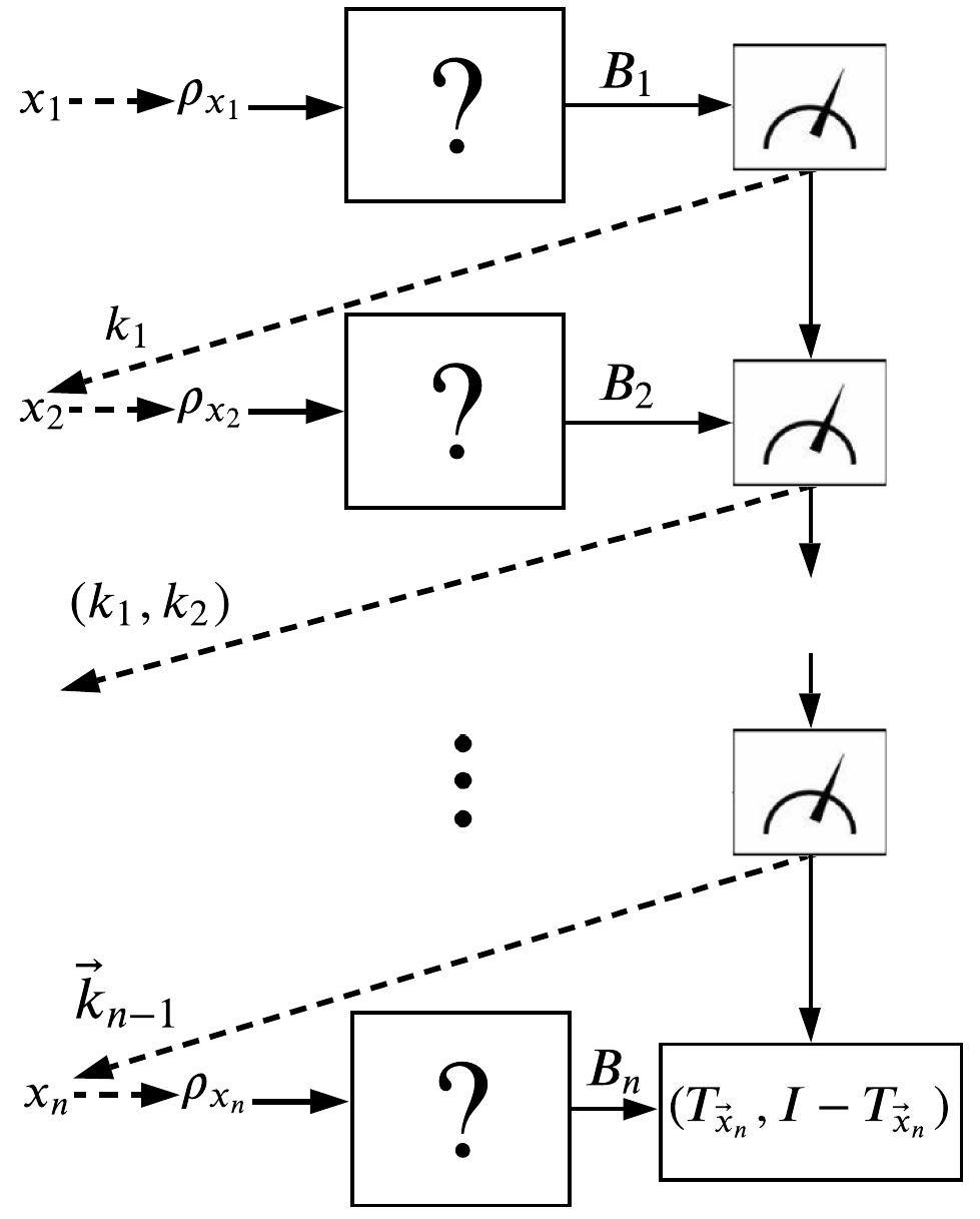
To study the adaptive discrimination of cq-channels, the general strategy for discrimination of qq-channels in Sec. I should be tailored to the cq-channels. We argue that the most general strategy in Sec. I can w.l.o.g. be replaced by the kind of strategy with the instrument and only classical feed-forward when the hypotheses are a pair of cq-channels. This in particular will turn out to be crucial since we consider general cq-channels with arbitrary (continuous) input alphabet.

The first input is chosen subject to the distribution $p_{X_{1}}(x_{1})$. The receiver receives the output $\rho_{x_{1}}$ or $\sigma_{x_{1}}$ on $B_{1}$. Dependently of the input $x_{1}$, the receiver applies the first quantum instrument $B_{1}\to K_{1}R_{2}$, where $R_{2}$ is the quantum memory system and $K_{1}$ is the classical outcome. The receiver sends the outcome $K_{1}$ to the sender. Then, the sender choose the second input $x_{2}$ according to the conditional distribution $p_{X_{2}|X_{1},K_{1}}(x_{2}|x_{1},k_{1})$. The receiver receives the second output $\rho_{x_{2}}$ or $\sigma_{x_{2}}$ on $B_{2}$. Dependently of the previous outcome $k_{1}$ and the previous inputs $x_{1},x_{2}$, the receiver applies the second quantum instrument $B_{2}R_{2}\to K_{2}R_{3}$, and sends the outcome $K_{2}$ to the sender. The third input is chosen as the distribution $p_{X_{3}|X_{1},X_{2},K_{1},K_{2}}(x_{2}|x_{1},x_{2},k_{1},k_{2})$.

In the same way as the above, the $m$-th step is given as follows. The sender chooses the $m$-th input $x_{m}$ according to the conditional distribution $p_{X_{m}|\vec{X}_{m-1},\vec{K}_{m-1}}(x_{m}|\vec{x}_{m-1},\vec{k}_{m-1})$. The receiver receives the second output $\rho_{x_{m}}$ or $\sigma_{x_{m}}$ on $B_{m}$. The remaining processes need the following divided cases. For $m<n$, dependently of the previous outcomes $\vec{k}_{m-1}:=(k_{1},\ldots,k_{m-1})$ and the previous inputs $\vec{x}_{m}:=(x_{1},\ldots,x_{m})$, the receiver applies the $m$-th quantum instrument $\mathcal{E}_{m}:R_{m}B_{m}\to K_{m}R_{m+1}$, and sends the outcome $k_{m}$ to the sender. For $m=n$, dependently of the previous outcomes $\vec{K}_{n-1}$ and the previous inputs $\vec{X}_{n}$, the receiver measures the final state on ${R_{n}B_{n}}$ with the binary POVM $(T_{n|\vec{k}_{n-1},\vec{x}_{n}},I-T_{n|\vec{k}_{n-1},\vec{x}_{n}})$, where hypothesis $\mathcal{N}$ (resp. $\overline{\mathcal{N}}$) is accepted if and only if the first (resp. second) outcome clicks.

In the following, we denote the class of the above general strategies by $\bar{\mathbb{A}}^{c,0}$ because it can be considered that this strategy has no quantum memory in the input side and no quantum feedback. As a subclass, we focus on the class when no feedback is allowed and the input state deterministically is fixed to a single input $x$, which is denoted $\bar{\mathbb{P}}^{0}$.

Figure 4: Adaptive strategy for cq-channel discrimination. Solid and dashed lines denote flow of classical and quantum information, respectively. The classical outputs of PVMs are employed to decide the inputs adaptively, and leave a post-measurement state that can be accessed together with the next channel output.

V.1.2 Protocol with PVM for cq-channels

The general procedure for discriminating cq-channels can be rewritten as follows using PVMs.

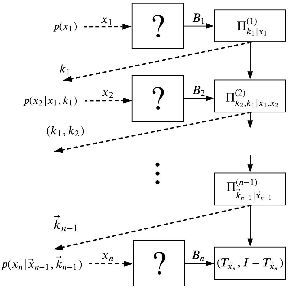
To start, Fig. 4 illustrates the general protocol with PVMs, which we shall describe now. In the following, according to Naimarks dilation theorem, in each $m$-th step, we choose a sufficiently large space $B_{m}$ including the original space $B_{m}$ such that the measurement is a PVM.

The first input is chosen subject to the distribution $p_{X_{1}}(x_{1})$. Then the output state is measured by a projection-valued measure (PVM) $\left\{\Pi_{k_{1}|x_{1}}^{(1)}\right\}_{k_{1}}$ on $B_{1}$. The second input is then chosen according to the distribution $p_{X_{2}|X_{1},K_{1}}(x_{2}|x_{1},k_{1})$. Then, a PVM $\left\{\Pi_{k_{2},k_{1}|x_{1},x_{2}}^{(2)}\right\}_{k_{1},k_{2}}$ is made on $B_{1}B_{2}$, which satisfies $\sum_{k_{2}}\Pi_{k_{2},k_{1}|x_{1},x_{2}}^{(2)}=\Pi_{k_{1}|x_{1}}^{(1)}\otimes I$. The third input is chosen as the distribution $p_{X_{3}|X_{1},X_{2},K_{1},K_{2}}(x_{3}|x_{1},x_{2},k_{1},k_{2})$, etc. Continuing, the $m$-th step is given as follows. the sender chooses the $m$-th input $x_{m}$ according to the conditional distribution $p_{X_{m}|\vec{X}_{m-1},\vec{K}_{m-1}}(x_{m}|\vec{x}_{m-1},\vec{k}_{m-1})$. The receiver receives the $m$-th output $\rho_{x_{m}}$ or $\sigma_{x_{m}}$ on $B_{m}$.

The description of the remaining processing requires that we distinguish two cases.

• For $m<n$, depending on the previous outcomes $\vec{k}_{m-1}=(k_{1},\ldots,k_{m-1})$ and the previous inputs $\vec{x}_{m}=(x_{1},\ldots,x_{m})$, as the $m$-th projective measurement, the receiver applies a PVM $\left\{\Pi_{\vec{k}_{m}|\vec{x}_{m}}^{(m)}\right\}_{\vec{k}_{m}}$ on $B_{1}B_{2}\cdots B_{m}$, which satisfies the condition $\sum_{k_{m}}\Pi_{\vec{k}_{m}|\vec{x}_{m}}^{(m)}=\Pi_{\vec{k}_{m-1}|\vec{x}_{m-1}}^{(m-1)}\otimes I$. He sends the outcome $k_{m}$ to the sender.

• For $m=n$, dependently of the inputs $\vec{x}_{n}$, the receiver measures the final state on $B_{1}B_{2}\cdots B_{n}$ with the binary POVM $(T_{\vec{x}_{n}},I-T_{\vec{x}_{n}})$ on $B_{1}B_{2}\cdots B_{n}$, where hypothesis $\mathcal{N}$ (resp. $\overline{\mathcal{N}}$) is accepted if and only if the first (resp. second) outcome clicks.

Proposition 8.

Any general procedure given in Subsubsection V.1.1 can be rewritten in the above form.

Proof.

Recall Corollary 7 given in Section IV. Due to Corollary 7, when the Hilbert space $B$ can be chosen sufficiently large, any state reduction written by a cp-map valued measure $\{\Gamma_{k_{1}|x_{1}}\}_{k_{1}}$ can also be written as the combination of a PVM $\{\Pi_{k_{1}|x_{1}}^{(1)}\}_{k_{1}}$ and a state change by a cptp map $\Lambda_{k_{1},x_{1}}$ depending on the measurement outcome $k_{1}$ such that $\Gamma_{k_{1}|x_{1}}(\rho)=\Lambda_{k_{1},x_{1}}(\Pi_{k_{1}|x_{1}}^{(1)}\rho\Pi_{k_{1}|x_{1}}^{(1)})$ for $k_{1},x_{1}$. Hence, we have $\Gamma_{k_{1}|x_{1}}(\rho)=\Lambda_{k_{1},x_{1}}(\Pi_{k_{1}|x_{1}}\rho\Pi_{k_{1}|x_{1}})$ for $k_{1},x_{1}$.

Then, we treat the cptp map $\Lambda_{k_{1},x_{1}}$ as a part of the next measurement. Let $\{\Gamma_{k_{2}|x_{1},x_{2},k_{1}}\}_{k_{2}}$ be the quantum instrument to describe the second measurement. We define the quantum instrument $\{\overline{\Gamma}_{k_{2}|x_{1},x_{2},k_{1}}\}_{k_{2}}$ as $\overline{\Gamma}_{k_{2}|x_{1},x_{2},k_{1}}(\rho):={\Gamma}_{k_{2}|x_{1},x_{2},k_{1}}(\Lambda_{k_{1},x_{1}}(\rho))$. Applying Corollary 7 to the quantum instrument $\{\overline{\Gamma}_{k_{2}|x_{1},x_{2},k_{1}}\}_{k_{2}}$, we choose the PVM $\{\Pi_{k_{2}|x_{1},x_{2},k_{1}}^{(2)}\}_{k_{2}}$ on $\mathop{\rm Im}\Pi_{k_{1}|x_{1}}^{(1)}\otimes B_{2}$ and the state change by a cptp map $\Lambda_{k_{1},k_{2},x_{1},x_{2}}$ depending on the measurement outcome $k_{2}$ to satisfy (14). Since $\sum_{k_{1},k_{2}}\Pi_{k_{2}|x_{1},x_{2},k_{1}}^{(2)}$ is the identity on $B_{1}B_{2}$, setting $\Pi_{k_{1},k_{2}|x_{1},x_{2}}^{(2)}:=\Pi_{k_{2}|x_{1},x_{2},k_{1}}^{(2)}$, we define the PVM $\{\Pi_{k_{1},k_{2}|x_{1},x_{2}}^{(2)}\}_{k_{1},k_{2}}$ on $B_{1}B_{2}$.

In the same way, for the $m$-th step, using a quantum instrument $\{\Gamma_{k_{m}|\vec{x}_{m},\vec{k}_{m-1}}\}_{k_{m}}$, cptp maps $\Lambda_{\vec{k}_{m-1},\vec{x}_{m-1}}$, and Corollary 7, we define the PVM $\{\Pi_{k_{m}|\vec{x}_{m},\vec{k}_{m-1}}^{(m)}\}_{k_{m}}$ on $\mathop{\rm Im}\Pi_{\vec{k}_{m-1}|\vec{x}_{m-1}}^{(m-1)}\otimes B_{m}$ and the state change by cptp maps $\Lambda_{\vec{k}_{m},\vec{x}_{m}}$. Then, setting $\Pi_{\vec{k}_{m}|\vec{x}_{m}}^{(m)}:=\Pi_{k_{m}|\vec{x}_{m},\vec{k}_{m-1}}^{(m)}$, we define the PVM $\{\Pi_{\vec{k}_{m}|\vec{x}_{m}}^{(m)}\}_{\vec{k}_{m}}$ on $B_{1}B_{2}\cdots B_{m}$.

In the $n$-th step, i.e., the final step, using the binary POVM $(T_{n|\vec{k}_{n-1},\vec{x}_{n}},I-T_{n|\vec{k}_{t-1},\vec{x}_{n}})$ and cptp maps $\Lambda_{\vec{k}_{n-1},\vec{x}_{n-1}}$, we define the binary POVM $(T_{\vec{x}_{n}},I-T_{\vec{x}_{n}})$ on $B_{1}B_{2}\cdots B_{n}$ as follows.

$$T_{\vec{x}_{n}}:=\sum_{\vec{k}_{n}}\Lambda_{\vec{k}_{n-1},\vec{x}_{n-1}}^{\dagger}(T_{n|\vec{k}_{n-1},\vec{x}_{n}}),$$ (17)

where $\Lambda_{\vec{k}_{n-1},\vec{x}_{n-1}}^{\dagger}$ is defined as $\operatorname{Tr}\Lambda_{\vec{k}_{n-1},\vec{x}_{n-1}}(\rho)X=\operatorname{Tr}\rho\Lambda_{\vec{k}_{n-1},\vec{x}_{n-1}}^{\dagger}(X)$. In this way, the general protocol given in Subsubsection V.1.1 has been converted a protocol given in this subsection. ∎

It is implicit that the projective measurement $\{\Pi_{\vec{k}_{m}|\vec{x}_{m}}^{(m)}\}_{\vec{k}_{m}}$ includes first projecting the output from the quantum memory onto a subspace spanned by $\{\Pi_{\vec{k}_{m}-1|\vec{x}_{m-1}}^{(m-1)}\}_{\vec{k}_{m-1}}$, and then finding $\vec{k}_{m}$ in the entire subspace of $\mathop{\rm Im}\Pi^{(m-1)}_{\vec{k}_{m-1}|\vec{x}_{m-1}}\otimes B$. Hence, $\{\Pi_{\vec{k}_{m}|\vec{k}_{m-1},\vec{x}_{m-1}}^{(m)}\}_{\vec{k}_{m}}$ can be regarded as a PVM on $B^{\otimes m}$ and from the construction

$$\sum_{k_{m}}\Pi^{(m)}_{\vec{k}_{m}|\vec{x}_{m}}=(\Pi^{(1)}_{k_{1}|x_{1}}\otimes I^{\otimes(m-1)})\cdots(\Pi_{\vec{k}_{m-1}|\vec{x}_{m-1}}^{(m-1)}\otimes I),$$

which shows that the PVMs commute.

Notice also that

$$\Pi_{\vec{k}_{n-1}|\vec{x}_{n-1}}^{(n-1)}\leq\Pi_{\vec{k}_{n-2}|\vec{x}_{n-2}}^{(n-2)}\otimes I\leq\cdots\leq\Pi_{\vec{k}_{1}|\vec{x}_{1}}^{(1)}\otimes I^{\otimes(n-2)}.$$

When the true channel is $\mathcal{N}:x\rightarrow\rho_{x}$, the state before the final measurement is

$$\rho^{(n)}\coloneqq\sum_{\vec{x}_{n},\vec{k}_{n-1}} p_{X_{1}}(x_{1})\cdots p_{{X}_{n}|\vec{X}_{n-1},\vec{K}_{n-1}}({x}_{n}|\vec{x}_{n-1},\vec{k}_{n-1})$$

$$\left(\Pi_{\vec{k}_{n-1}|\vec{x}_{n-1}}^{(n-1)}\big{(}\rho_{x_{1}}\otimes\cdots\otimes\rho_{x_{n}}\big{)}\Pi_{\vec{k}_{n-1}|\vec{x}_{n-1}}^{(n-1)}\otimes\outerproduct{\vec{x}_{n}}{\vec{x}_{n}}\right),$$ (18)

where here we need to store the information for inputs $\vec{x}_{n}$. Similarly, when the true channel is $\overline{\mathcal{N}}:x\rightarrow\sigma_{x}$

$$\sigma^{(n)}\coloneqq\sum_{\vec{x}_{n},\vec{k}_{n-1}} p_{X_{1}}(x_{1})\cdots p_{{X}_{n}|\vec{X}_{n-1},\vec{K}_{n-1}}({x}_{n}|\vec{x}_{n-1},\vec{k}_{n-1})$$

$$\left(\Pi_{\vec{k}_{n-1}|\vec{x}_{n-1}}^{(n-1)}\big{(}\sigma_{x_{1}}\otimes\cdots\otimes\sigma_{x_{n}}\big{)}\Pi_{\vec{k}_{n-1}|\vec{x}_{n-1}}^{(n-1)}\otimes\outerproduct{\vec{x}_{n}}{\vec{x}_{n}}\right).$$ (19)

A test of the hypotheses $\{\mathcal{N},\overline{\mathcal{N}}\}$ on the true channel is a two-valued POVM $\{T_{n},I-T_{n}\}$, where $T_{n}$ is given as a Hermitian operator $\sum_{\vec{x}_{n}}T_{\vec{x}_{n}}\otimes|\vec{x}_{n}\rangle\langle\vec{x}_{n}|$ on $B^{\otimes n}\otimes X^{\otimes n}$ satisfying $0\leq T_{n}\leq I$. Overall, our strategy to distinguish the channels $\{\mathcal{N},\overline{\mathcal{N}}\}$ when $n$ independent uses of each are available, is given by the triple $\mathcal{T}_{n}:=(\{\Pi^{(m)}_{\vec{k}_{m}|\vec{x}_{m}}\}_{m=1}^{n-1},\{p_{{X}_{m}|\vec{X}_{m-1},\vec{K}_{m-1}}\}_{m=1}^{n},T_{n})$. The $n$-copy error probabilities of type I and type II are respectively as follows

$$\alpha_{n}({\mathcal{N}}\|\overline{\mathcal{N}}|\mathcal{T}_{n}) \coloneqq\operatorname{Tr}\rho^{(n)}(I-T_{n}),$$

$$\beta_{n}({\mathcal{N}}\|\overline{\mathcal{N}}|\mathcal{T}_{n}) \coloneqq\operatorname{Tr}\sigma^{(n)}T_{n}.$$

The generalized Chernoff and Hoeffding quantities introduced in the introduction read as follows in the present cq-channel case for a given class $\bar{\mathbb{S}}\subset\bar{\mathbb{A}}^{c,0}$ :

$$C^{\bar{\mathbb{S}}}(a,b|\mathcal{N}\|\overline{\mathcal{N}}) \coloneqq\sup_{\{\mathcal{T}_{n}\}}\left\{\liminf_{n\rightarrow\infty}-\frac{1}{n}\log\left(2^{an}\alpha_{n}({\mathcal{N}}\|\overline{\mathcal{N}}|\mathcal{T}_{n})+2^{bn}\beta_{n}({\mathcal{N}}\|\overline{\mathcal{N}}|\mathcal{T}_{n})\right)\right\},$$ (20)

$$B_{e}^{\bar{\mathbb{S}}}(r|\mathcal{N}\|\overline{\mathcal{N}}) \coloneqq\sup_{\{\mathcal{T}_{n}\}}\left\{\liminf_{n\rightarrow\infty}-\frac{1}{n}\log\left(\alpha_{n}({\mathcal{N}}\|\overline{\mathcal{N}}|\mathcal{T}_{n})\right)\bigg{|}\liminf_{n\rightarrow\infty}-\frac{1}{n}\log\left(\beta_{n}({\mathcal{N}}\|\overline{\mathcal{N}}|\mathcal{T}_{n})\right)\geq r\right\},$$ (21)

where $a$, $b$, are arbitrary real numbers and $r$ is an arbitrary non-negative number.

V.2 Auxiliary results and techniques

We set $\rho_{x}:=\mathcal{N}(x)$ and $\sigma_{x}:=\overline{\mathcal{N}}(x)$, and define

$$C(a,b):= \sup_{x}\sup_{0\leq\alpha\leq 1}(1-\alpha)D_{\alpha}(\rho_{x}\|\sigma_{x})-\alpha a-(1-\alpha)b$$

$$= \sup_{0\leq\alpha\leq 1}(1-\alpha)D_{\alpha}(\mathcal{N}\|\overline{\mathcal{N}})-\alpha a-(1-\alpha)b,$$ (22)

$$B(r):= \sup_{x}\sup_{0\leq\alpha\leq 1}\frac{\alpha-1}{\alpha}\big{(}r-D_{\alpha}(\rho_{x}\|\sigma_{x})\big{)}=\sup_{0\leq\alpha\leq 1}\frac{\alpha-1}{\alpha}\big{(}r-D_{\alpha}(\mathcal{N}\|\overline{\mathcal{N}})\big{)},$$ (23)

where $D_{\alpha}(\mathcal{N}\|\overline{\mathcal{N}}):=\sup_{x}D_{\alpha}(\rho_{x}\|\sigma_{x})$ and $D_{\alpha}(\rho_{x}\|\sigma_{x})\coloneqq\frac{1}{\alpha-1}\log\operatorname{Tr}\rho_{x}^{\alpha}\sigma_{x}^{1-\alpha}$ is a quantum extension of the Rényi relative entropy.

Since $D_{\alpha}(\rho_{x}\|\sigma_{x})$ is monotonically increasing for $\alpha$, $D_{\alpha}(\mathcal{N}\|\overline{\mathcal{N}})$ is monotonically increasing for $\alpha$. Thus,

$$\lim_{\alpha\to 1}D_{\alpha}(\mathcal{N}\|\overline{\mathcal{N}}) =\sup_{0\leq\alpha\leq 1}D_{\alpha}(\mathcal{N}\|\overline{\mathcal{N}})=\sup_{0\leq\alpha\leq 1}\sup_{x}D_{\alpha}(\rho_{x}\|\sigma_{x})$$

$$=\sup_{x}\sup_{0\leq\alpha\leq 1}D_{\alpha}(\rho_{x}\|\sigma_{x})=\sup_{x}D(\rho_{x}\|\sigma_{x})=D(\mathcal{N}\|\overline{\mathcal{N}}).$$

Before stating the main results of this section we shall study the $B(r)$ function further. Since the $B(r)$ function is monotonically decreasing in $r$, $B(D(\mathcal{N}\|\overline{\mathcal{N}}))=0$. To find $B(0)$, since $\frac{1-\alpha}{\alpha}D_{\alpha}(\mathcal{N}\|\overline{\mathcal{N}})=D_{1-\alpha}(\overline{\mathcal{N}}\|\mathcal{N})$, we infer that $\frac{1-\alpha}{\alpha}D_{\alpha}(\mathcal{N}\|\overline{\mathcal{N}})$ is monotonically decreasing for $\alpha$, and $D(\overline{\mathcal{N}}\|\mathcal{N})=\lim_{\alpha\to 0}\frac{1-\alpha}{\alpha}D_{\alpha}(\mathcal{N}\|\overline{\mathcal{N}})$. Hence, $B(0)=D(\overline{\mathcal{N}}\|\mathcal{N})$, and $B(r)<D(\overline{\mathcal{N}}\|\mathcal{N})$ for $r>0$.

The following lemma states the continuity of the $B(r)$ function, of which we give two different proofs. The first proof uses the known facts for the case of two states, and the cq-channel case is reduced to the former by general statements from convex analysis. The second proof is rather more ad-hoc and relies on peculiarities of the functions at hand.

Lemma 9.

The function (Hoeffding expoent) $B(r)$ is continuous in $r$, i.e. for any non-negative real number $r_{0}$,

$$\lim_{r\to r_{0}}B(r)=B(r_{0}).$$ (24)

Proof.

The crucial difficulty in this lemma is that unlike previous works, here we allow that $|\mathcal{X}|$ is infinite. Note that in the case of a finite alphabet, we just need to note the role of the channel (as opposed to states): it is a supremum over channel inputs $x\in\mathcal{X}$, so a preliminary task is to prove that for a fixed $x$, i.e. a pair of states $\rho_{x}$ and $\sigma_{x}$, the Hoeffding function is continuous. This is already known (Ogawa-Hayashi, , Lemma 1) and follows straightforwardly from the convexity and monotonicity of the Hoeffding function. After that, the channel’s Hoeffding function is the maximum over finitely many continuous functions and so continuous. However, when the alphabet size is infinite, the supremum of infinitely many continuous functions is not necessarily continuous. Nevertheless, it inherits the convexity of the functions for each $x$, cf. (convexbook, , Cor. 3.2.8). Since the function is defined on the non-negative reals $\mathbb{R}_{\geq 0}$, it is continuous for all $r_{0}>0$, by the well-known and elementary fact that a convex function on an interval is continuous on its interior. It only remains to prove the continuity at $r_{0}=0$; to this end consider swapping null and alternative hypotheses and denote the corresponding Hoeffding exponent by $\overline{B}(r)$. We then find that $\overline{B}(r)$ is the inverse function of $B(r)$. Since $\overline{B}(r)$ is continuous even when it is equal to zero, i.e. at $r=D(\overline{\mathcal{N}}\|\mathcal{N})$, we conclude $B(r)$ is continuous at $r=0$ and $B(0)=D(\overline{\mathcal{N}}\|\mathcal{N})$. ∎

Alternative proof of Lemma 9.

Given $r_{0}>0$, there exist $\alpha_{0}\in(0,1)$ and a sequence $\alpha_{n}$ such that $\alpha_{n}\to\alpha_{0}$ and $\lim_{n\to\infty}\frac{\alpha_{n}-1}{\alpha_{n}}\big{(}r_{0}-D_{\alpha_{n}}(\mathcal{N}\|\overline{\mathcal{N}})\big{)}=B(r_{0})$. Hence, we have $\sup_{\frac{\alpha_{0}}{2}\leq\alpha\leq 1}\frac{\alpha-1}{\alpha}\big{(}r_{0}-D_{\alpha}(\mathcal{N}\|\overline{\mathcal{N}})\big{)}=B(r_{0})$. For $r>r_{0}$, the above supremum with $r$ is realized by $\alpha\in[\frac{\alpha_{0}}{2},1]$. That is, $\sup_{\frac{\alpha_{0}}{2}\leq\alpha\leq 1}\frac{\alpha-1}{\alpha}\big{(}r-D_{\alpha}(\mathcal{N}\|\overline{\mathcal{N}})\big{)}=B(r)$. In the range $[\frac{\alpha_{0}}{2},1]$, $\frac{\alpha-1}{\alpha}\big{(}r-D_{\alpha}(\mathcal{N}\|\overline{\mathcal{N}})\big{)}$ is uniformly continuous for $r$, we have (24). The proof implies that larger $r$ corresponds to larger $\alpha$. To show this, we introduce $k(\alpha)$ as the first derivative of $D_{\alpha}(\mathcal{N}\|\overline{\mathcal{N}})$, which crucially does not depend on $r$. The other term, $\frac{\alpha-1}{\alpha}r$, has derivative $\frac{-r}{\alpha^{2}}$, so the condition for the maximum is $\frac{-r}{\alpha^{2}}+k(\alpha)=0$. Now consider the optimal value $\alpha_{0}$ for a certain $r_{0}>0$, so the above equation is satisfied for $r_{0}$ and $\alpha_{0}$. If we now consider $r>r_{0}$, the same $\alpha=\alpha_{0}$ gives a negative derivative, which means that we make the objective function larger by increasing $\alpha\geq\alpha_{0}$, which is where the optimal value must lie. Continuity at $r=0$ follows similar to the previous proof. ∎

The combination of Lemma 9 and the above observation guarantees that the map $r\mapsto B(r)-r$ is a continuous and strictly decreasing function from $[0,D(\mathcal{N}\|\overline{\mathcal{N}})]$ to $[-D(\mathcal{N}\|\overline{\mathcal{N}}),D(\overline{\mathcal{N}}\|\mathcal{N})]$. Hence, when real numbers $a,b$ satisfy $-D(\mathcal{N}\|\overline{\mathcal{N}})\leq a-b\leq D(\overline{\mathcal{N}}\|\mathcal{N})$, there exists $r_{a,b}\in[0,D(\mathcal{N}\|\overline{\mathcal{N}})]$ such that $B(r_{a,b})-r_{a,b}=a-b$.

Lemma 10.

When real numbers $a,b$ satisfy $-D(\mathcal{N}\|\overline{\mathcal{N}})\leq a-b\leq D(\overline{\mathcal{N}}\|\mathcal{N})$, then we have

$$C(a,b)=r_{a,b}-b=B(r_{a,b})-a.$$ (25)

Proof.

Definition of $C(a,b)$, Eq. (22), implies that $C(a-c,b-c)=C(a,b)+c$. Hence, it is sufficient to show that for $r\in[0,D(\mathcal{N}\|\overline{\mathcal{N}})]$:

$$C(B(r),r)=0.$$ (26)

$$C(B(r),r) =\sup_{0\leq\alpha\leq 1}(1-\alpha)D_{\alpha}(\mathcal{N}\|\overline{\mathcal{N}})-\alpha B(r)-(1-\alpha)r$$

$$=\sup_{0\leq\alpha\leq 1}\alpha\Big{(}\frac{\alpha-1}{\alpha}\big{(}r-D_{\alpha}(\mathcal{N}\|\overline{\mathcal{N}})\big{)}-B(r)\Big{)}=0,$$

where the last equality follows since $\frac{\alpha-1}{\alpha}\big{(}r-D_{\alpha}(\mathcal{N}\|\overline{\mathcal{N}})\big{)}\leq B(r)$ for $0\leq\alpha\leq 1$. ∎

Our approach consists of associating suitable classical channels to the given cq-channels, and noting the lessons learned about adaptive strategy for discrimination of classical channels in 5165184 . Our proof methodology however, is also novel for the classical case. The following Lemmas 11 and 12 addresses these matters; the former is verified easily and its proof is omitted, and the latter is more involved and is the key to our developments.

Lemma 11.

Consider the cq-channels $\mathcal{N}:x\rightarrow\rho_{x}$ and $\overline{\mathcal{N}}:x\rightarrow\sigma_{x}$ with input alphabet $\mathcal{X}$ and output density operators on Hilbert space $B$. Let the eigenvalue decompositions of the output operators be as follows:

$$\rho_{x}=\sum_{i}\lambda_{i}^{x}\outerproduct{u_{i}^{x}}{u_{i}^{x}},$$ (27)

$$\sigma_{x}=\sum_{j}\mu_{j}^{x}\outerproduct{v_{j}^{x}}{v_{j}^{x}}.$$ (28)

Define

$$\Gamma_{x}(i,j)\coloneqq\lambda_{i}^{x}\left|\bra{v_{j}^{x}}\ket{u_{i}^{x}}\right|^{2},$$ (29)

$$\overline{\Gamma}_{x}(i,j)\coloneqq\mu_{i}^{x}\left|\bra{v_{j}^{x}}\ket{u_{i}^{x}}\right|^{2}.$$ (30)

First, $\Gamma_{x}(i,j)$ and $\overline{\Gamma}_{x}(i,j)$ form (conditional) probability distributions on the range $\{(i,j)\}$ of the pairs $(i,j)$, i.e. for all pair of indexes $(i,j)$, we have $\Gamma_{x}(i,j)\geq 0,\overline{\Gamma}_{x}(i,j)\geq 0$ and $\sum_{(i,j)}\Gamma_{x}(i,j)=\sum_{(i,j)}\overline{\Gamma}_{x}(i,j)=1$. One can think of these distributions as classical channels. Second, we have

$$D_{\alpha}(\rho_{x}\|\sigma_{x})=D_{\alpha}(\Gamma_{x}\|\overline{\Gamma}_{x}),$$

which implies [see Eq. (23)]

$$\phantom{==}B(r)=\sup_{x}\sup_{0\leq\alpha\leq 1}\frac{\alpha-1}{\alpha}\big{(}r-D_{\alpha}(\Gamma_{x}\|\overline{\Gamma}_{x})\big{)}.\phantom{==}\square$$ (31)

Note that any extensions of the operators $\{\rho_{x},\sigma_{x}\}$ (not just i.i.d.) correspond to the classical extensions by distributions $\Gamma_{x}(i,j)$ and $\overline{\Gamma}_{x}(i,j)$. Define

$$\Gamma_{\vec{x}_{n}}^{n}(\vec{i}_{n},\vec{j}_{n})\coloneqq\Gamma_{x_{1}}(i_{1},j_{1})\cdots\Gamma_{x_{n}}(i_{n},j_{n}),$$

$$\overline{\Gamma}_{\vec{x}_{n}}^{n}(\vec{i}_{n},\vec{j}_{n})\coloneqq\overline{\Gamma}_{x_{1}}(i_{1},j_{1})\cdots\overline{\Gamma}_{x_{n}}(i_{n},j_{n}).$$

Then, we have the following lemma.

Lemma 12.

$$E_{a,b,n}^{Q}\coloneqq\min_{T}2^{an}\operatorname{Tr}(I-T)\rho^{(n)}+2^{bn}\operatorname{Tr}T\sigma^{(n)}\geq\frac{1}{2}E_{a,b,n}^{C},$$

where

$$E_{a,b,n}^{C}\coloneqq \min_{q_{X_{1}},\ldots,q_{X_{n}K_{n-1}|\vec{K}_{n-2}\vec{X}_{n-1}\vec{I}_{n-1}\vec{J}_{n-1}}}$$

$$\sum_{\vec{x}_{n},\vec{j}_{n},\vec{i}_{n},\vec{k}_{n-1}}q_{X_{1}}(x_{1})\ldots q_{X_{n}K_{n-1}|\vec{K}_{n-2}\vec{X}_{n-1}\vec{I}_{n-1}\vec{J}_{n-1}}(x_{n},k_{n-1}|\vec{k}_{n-2},\vec{x}_{n-1},\vec{i}_{n-1},\vec{j}_{n-1})$$

$$\hskip 56.9055pt\cdot\min\left\{2^{an}\Gamma_{\vec{x}_{n}}^{n}(\vec{i}_{n},\vec{j}_{n}),2^{bn}\overline{\Gamma}_{\vec{x}_{n}}^{n}(\vec{i}_{n},\vec{j}_{n})\right\}.$$

Proof.

Let

$$\ket{u_{\vec{i}_{n}}^{\vec{x}_{n}}}\coloneqq\ket{u_{i_{1}}^{x_{1}},\ldots,u_{{i}_{n}}^{{x}_{n}}},~{}\lambda_{\vec{i}_{n}}^{\vec{x}_{n}}\coloneqq\lambda_{i_{1}}^{x_{1}},\cdots\lambda_{{i}_{n}}^{{x}_{n}},$$

$$\ket{v_{\vec{j}_{n}}^{\vec{x}_{n}}}\coloneqq\ket{v_{j_{1}}^{x_{1}},\ldots,v_{{j}_{n}}^{{x}_{n}}},~{}\mu_{\vec{j}_{n}}^{\vec{x}_{n}}\coloneqq\mu_{j_{1}}^{x_{1}},\cdots\mu_{{j}_{n}}^{{x}_{n}}.$$

Consider $\min_{T}2^{an}\operatorname{Tr}(I-T)\rho^{(n)}+2^{bn}\operatorname{Tr}T\sigma^{(n)}$; it is sufficient to consider $T$ to a projective measurement because the minimum can be attained when $T$ is a projection onto the subspace that is given as the linear span of eigenspaces corresponding to negative eigenvalues of $-2^{an}\rho^{(n)}+2^{bn}\sigma^{(n)}$. For a given $\vec{x}_{n}$, the final decision is given as the projection $T_{\vec{x}_{n}}$ on the image of the projection $\Pi_{\vec{k}_{n-1}|\vec{x}_{n-1}}^{(n-1)}$ on $B^{\otimes n}$ depending on $\vec{x}_{n}$. Since $\rho^{(n)}$ and $\sigma^{(n)}$ both commute with the projection $\Pi_{\vec{k}_{n-1}|\vec{x}_{n-1}}^{(n-1)}$, without loss of generality, we can assume that the projection $T_{\vec{x}_{n}}$ is also commutative with $\Pi_{\vec{k}_{n-1}|\vec{x}_{n-1}}^{(n-1)}$. Then, the final decision operator $T_{n}$ is given as the projection $T_{n}\coloneqq\sum_{\vec{x}_{n}}T_{\vec{x}_{n}}\otimes|\vec{x}_{n}\rangle\langle\vec{x}_{n}|$.

We expand the first term as follows:

$$\operatorname{Tr} (I-T_{n})\rho^{(n)}$$

$$=\sum_{\vec{x}_{n},\vec{k}_{n-1}}\operatorname{Tr}(I-T_{\vec{x}_{n}})p_{X_{1}}(x_{1})\cdots p_{{X}_{n}|\vec{X}_{n-1},\vec{K}_{n-1}}({x}_{n}|\vec{x}_{n-1},\vec{k}_{n-1})\Pi_{\vec{k}_{n-1}|\vec{x}_{n-1}}^{(n-1)}\big{(}\rho_{x_{1}}\otimes\cdots\otimes\rho_{x_{n}}\big{)}\Pi_{\vec{k}_{n-1}|\vec{x}_{n-1}}^{(n-1)}$$

$$=\sum_{\vec{x}_{n},\vec{k}_{n-1}}\operatorname{Tr}(I-T_{\vec{x}_{n}})^{2}p_{X_{1}}(x_{1})\cdots p_{{X}_{n}|\vec{X}_{n-1},\vec{K}_{n-1}}({x}_{n}|\vec{x}_{n-1},\vec{k}_{n-1})\Pi_{\vec{k}_{n-1}|\vec{x}_{n-1}}^{(n-1)}\big{(}\rho_{x_{1}}\otimes\cdots\otimes\rho_{x_{n}}\big{)}\Pi_{\vec{k}_{n-1}|\vec{x}_{n-1}}^{(n-1)}$$

$$=\sum_{\vec{x}_{n},\vec{k}_{n-1}}\operatorname{Tr}(I-T_{\vec{x}_{n}})\sum_{\vec{j}_{n}}\outerproduct{v_{\vec{j}_{n}}^{\vec{x}_{n}}}{v_{\vec{j}_{n}}^{\vec{x}_{n}}}(I-T_{\vec{x}_{n}})p_{X_{1}}(x_{1})\cdots p_{{X}_{n}|\vec{X}_{n-1},\vec{K}_{n-1}}({x}_{n}|\vec{x}_{n-1},\vec{k}_{n-1})$$

$$\hskip 270.30118pt\cdot\Pi_{\vec{k}_{n-1}|\vec{x}_{n-1}}^{(n-1)}\big{(}\rho_{x_{1}}\otimes\cdots\otimes\rho_{x_{n}}\big{)}\Pi_{\vec{k}_{n-1}|\vec{x}_{n-1}}^{(n-1)}$$

$$=\sum_{\vec{x}_{n},\vec{j}_{n},\vec{i}_{n},\vec{k}_{n-1}}p_{X_{1}}(x_{1})\cdots p_{{X}_{n}|\vec{X}_{n-1},\vec{K}_{n-1}}({x}_{n}|\vec{x}_{n-1},\vec{k}_{n-1})\lambda_{\vec{i}_{n}}^{\vec{x}_{n}}\left|\bra{u_{\vec{i}_{n}}^{\vec{x}_{n}}}(I-T_{\vec{x}_{n}})\Pi_{\vec{k}_{n-1}|\vec{x}_{n-1}}^{(n-1)}\ket{v_{\vec{j}_{n}}^{\vec{x}_{n}}}\right|^{2},$$

where the first line follows from the definition of $T$, the second line is due to the fact that the final measurement can be chosen as a projective measurement, the third line follows because $\sum_{\vec{j}_{n}}\outerproduct{v_{\vec{j}_{n}}^{\vec{x}_{n}}}{v_{\vec{j}_{n}}^{\vec{x}_{n}}}=I^{\otimes n}$ and the last line is simple manipulation.

Similarly, we have

$$\operatorname{Tr}T\sigma^{(n)}=\sum_{\vec{x}_{n},\vec{j}_{n},\vec{i}_{n},\vec{k}_{n-1}}p_{X_{1}}(x_{1})\cdots p_{{X}_{n}|\vec{X}_{n-1},\vec{K}_{n-1}}({x}_{n}|\vec{x}_{n-1},\vec{k}_{n-1})\mu_{\vec{j}_{n}}^{\vec{x}_{n}}\left|\bra{u_{\vec{i}_{n}}^{\vec{x}_{n}}}T_{\vec{x}_{n}}\Pi_{\vec{k}_{n-1}|\vec{x}_{n-1}}^{(n-1)}\ket{v_{\vec{j}_{n}}^{\vec{x}_{n}}}\right|^{2}.$$

For $m\in[1:n]$, define

$$q_{X_{m}K_{m-1}|\vec{K}_{m-2}\vec{X}_{m-1}\vec{I}_{m-1}\vec{J}_{m-1}}(x_{m},k_{m-1}|\vec{x}_{m-1},\vec{k}_{m-2},\vec{i}_{m-1},\vec{j}_{m-1})$$

$$\coloneqq p_{{X}_{m}|\vec{X}_{m-1},\vec{K}_{m-1}}({x}_{m}|\vec{x}_{m-1},\vec{k}_{m-1})\frac{\left|\bra{u_{\vec{i}_{m-1}}^{\vec{x}_{m-1}}}\Pi_{\vec{k}_{m-1}|\vec{x}_{m-1}}^{(m-1)}\ket{v_{\vec{j}_{m-1}}^{\vec{x}_{m-1}}}\right|^{2}}{\left|\bra{u_{\vec{i}_{m-2}}^{\vec{x}_{m-2}}}\Pi_{\vec{k}_{m-2}|\vec{x}_{m-2}}^{(m-2)}\ket{v_{\vec{j}_{m-2}}^{\vec{x}_{m-2}}}\right|^{2}\cdot\left|\innerproduct{u_{{i}_{m-1}}^{{x}_{m-1}}}{v_{{j}_{m-1}}^{{x}_{m-1}}}\right|^{2}}.$$

Hence,

$$\min_{T}2^{bn} 2^{an}\operatorname{Tr}(I-T)\rho^{(n)}+2^{an}\operatorname{Tr}T\sigma^{(n)}$$

$$= \sum_{\vec{x}_{n},\vec{j}_{n},\vec{i}_{n},\vec{k}_{n-1}}p_{X_{1}}(x_{1})\cdots p_{{X}_{n}|\vec{X}_{n-1},\vec{K}_{n-1}}({x}_{n}|\vec{x}_{n-1},\vec{k}_{n-1})$$

$$\cdot\Big{(}2^{an}\lambda_{\vec{j}_{n}}^{\vec{x}_{n}}\left|\bra{u_{\vec{i}_{n}}^{\vec{x}_{n}}}(I-T_{\vec{x}_{n}})\Pi_{\vec{k}_{n-1}|\vec{x}_{n-1}}^{(n-1)}\ket{v_{\vec{j}_{n}}^{\vec{x}_{n}}}\right|^{2}+2^{bn}\mu_{\vec{i}_{n}}^{\vec{x}_{n}}\left|\bra{u_{\vec{i}_{n}}^{\vec{x}_{n}}}T_{\vec{x}_{n}}\Pi_{\vec{k}_{n-1}|\vec{x}_{n-1}}^{(n-1)}\ket{v_{\vec{j}_{n}}^{\vec{x}_{n}}}\right|^{2}\Big{)}$$

$$\geq \sum_{\vec{x}_{n},\vec{j}_{n},\vec{i}_{n},\vec{k}_{n-1}}p_{X_{1}}(x_{1})\cdots p_{{X}_{n}|\vec{X}_{n-1},\vec{K}_{n-1}}({x}_{n}|\vec{x}_{n-1},\vec{k}_{n-1})\min\left\{2^{an}\lambda_{\vec{i}_{n}}^{\vec{x}_{n}},2^{bn}\mu_{\vec{j}_{n}}^{\vec{x}_{n}}\right\}$$

$$\cdot\Big{(}\left|\bra{u_{\vec{i}_{n}}^{\vec{x}_{n}}}T_{\vec{x}_{n}}\Pi_{\vec{k}_{n-1}|\vec{x}_{n-1}}^{(n-1)}\ket{v_{\vec{j}_{n}}^{\vec{x}_{n}}}\right|^{2}+\left|\bra{u_{\vec{i}_{n}}^{\vec{x}_{n}}}(I-T_{\vec{x}_{n}})\Pi_{\vec{k}_{n-1}|\vec{x}_{n-1}}^{(n-1)}\ket{v_{\vec{j}_{n}}^{\vec{x}_{n}}}\right|^{2}\Big{)}$$

$$\stackrel{{\scriptstyle\text{(a)}}}{{\geq}} \sum_{\vec{x}_{n},\vec{j}_{n},\vec{i}_{n},\vec{k}_{n-1}}p_{X_{1}}(x_{1})\cdots p_{{X}_{n}|\vec{X}_{n-1},\vec{K}_{n-1}}({x}_{n}|\vec{x}_{n-1},\vec{k}_{n-1})\min\left\{2^{an}\lambda_{\vec{i}_{n}}^{\vec{x}_{n}},2^{bn}\mu_{\vec{j}_{n}}^{\vec{x}_{n}}\right\}$$

$$\cdot\frac{1}{2}\left|\bra{u_{\vec{i}_{n}}^{\vec{x}_{n}}}\Pi_{\vec{k}_{n-1}|\vec{x}_{n}}^{(n-1)}\ket{v_{\vec{j}_{n}}^{\vec{x}_{n}}}\right|^{2}$$

$$= \frac{1}{2}\sum_{\vec{x}_{n},\vec{j}_{n},\vec{i}_{n},\vec{k}_{n-1}}q_{X_{1}}(x_{1})\cdots q_{X_{n}K_{n-1}|\vec{K}_{n-2}\vec{X}_{n-1}\vec{I}_{n-1}\vec{J}_{n-1}}(x_{n}k_{n-1}|\vec{k}_{n-2}\vec{x}_{n-1}\vec{i}_{n-1}\vec{j}_{n-1})$$

$$\cdot\min\left\{2^{an}\Gamma_{\vec{x}_{n}}(\vec{i}_{n},\vec{j}_{n}),2^{bn}\overline{\Gamma}_{\vec{x}_{n}}(\vec{i}_{n},\vec{j}_{n})\right\},$$

where (a) follows from the relation $|\alpha|^{2}+|\beta|^{2}\geq\frac{1}{2}|\alpha+\beta|^{2}$. ∎

V.3 Main results

We are now in a position to present and prove our main result, the generalized Chernoff bound, as follows:

Theorem 13 (Generalized Chernoff bound).

For two cq-channels $\mathcal{N}$ and $\overline{\mathcal{N}}$, and for real numbers $a,b$ satisfying $-D(\mathcal{N}\|\overline{\mathcal{N}})\leq a-b\leq D(\overline{\mathcal{N}}\|\mathcal{N})$,

$$C^{\bar{\mathbb{A}}^{c,0}}(a,b|\mathcal{N}\|\overline{\mathcal{N}})=C^{\bar{\mathbb{P}}^{0}}(a,b|\mathcal{N}\|\overline{\mathcal{N}})=C(a,b)=r_{a,b}-b=B(r_{a,b})-a.$$

Proof.

For the direct part, i.e. that strategies in $\mathbb{P}^{0}$ achieve this exponent, the following non-adaptive strategy achieves $C(a,b)$. Consider the transmission of a letter $x$ on every channel use. Define the test $T_{n}$ as the projection to the eigenspace of the positive eigenvalues of $2^{na}\rho_{x}^{\otimes n}-2^{nb}\sigma_{x}^{\otimes n}$. Audenaert et al. Audenaert_2007 showed that

$$2^{na}\operatorname{Tr}[\rho_{x}^{\otimes n}(I-T_{n})]+2^{nb}\operatorname{Tr}[\sigma_{x}^{\otimes n}T_{n}] \leq\inf_{0\leq\alpha\leq 1}\operatorname{Tr}(2^{na}\rho_{x}^{\otimes n})^{\alpha}(2^{nb}\sigma_{x}^{\otimes n})^{1-\alpha}$$

$$=2^{-n\sup_{0\leq\alpha\leq 1}\big{(}(1-\alpha)D_{\alpha}(\rho_{x}\|\sigma_{x})-\alpha a-(1-\alpha)b\big{)}}.$$ (32)

Considering the optimization for $x$, we obtain the direct part.

For the converse part, since

$$C^{\bar{\mathbb{A}}^{c,0}}(a,b|\mathcal{N}\|\overline{\mathcal{N}})=C^{\bar{\mathbb{A}}^{c,0}}(B(r_{a,b}),r_{a,b}|\mathcal{N}\|\overline{\mathcal{N}})+B(r_{a,b})-a=C^{\bar{\mathbb{A}}^{c,0}}(B(r_{a,b}),r_{a,b}|\mathcal{N}\|\overline{\mathcal{N}})+r_{a,b}-b,$$

it is sufficient to show $C^{\bar{\mathbb{A}}^{c,0}}(B(r),r|\mathcal{N}\|\overline{\mathcal{N}})\geq 0$ for $r\in[0,D(\mathcal{N}\|\overline{\mathcal{N}})]$. Observe that

$$E_{a,b,n}^{C}=2^{an}\alpha_{n}(\Gamma\|\overline{\Gamma}|\mathcal{T}_{a,b,n})+2^{bn}\beta_{n}(\Gamma\|\overline{\Gamma}|\mathcal{T}_{a,b,n}),$$

where we let $\mathcal{T}_{a,b,n}$ be the optimal test to achieve $E_{a,b,n}^{C}$. We choose $a=B(r)$ and $b=r$ in Lemma 12. The combination of (31) and (5165184, , Eq. (16)) guarantees that

$$B_{e}^{\bar{\mathbb{A}}^{c,0}}(r|\Gamma\|\overline{\Gamma})=B(r).$$ (33)

Notice that the analysis in 5165184 does not assume any condition on the set $\mathcal{X}$. When

$$\liminf_{n\to\infty}\frac{1}{n}\log 2^{rn}\beta_{n}(\Gamma\|\overline{\Gamma}|\mathcal{T}_{B(r),r,n})<0,$$

then Eq. (33) implies

$$\liminf_{n\to\infty}\frac{1}{n}\log 2^{B(r)n}\alpha_{n}(\Gamma\|\overline{\Gamma}|\mathcal{T}_{B(r),r,n})\geq 0.$$

Hence, we have

$$\begin{split}\liminf_{n\to\infty}\frac{1}{n}\log E_{B(r),r,n}^{C}&=\max\left\{\liminf_{n\to\infty}\frac{1}{n}\log 2^{rn}\beta_{n}(\Gamma\|\overline{\Gamma}|\mathcal{T}_{B(r),r,n})\right.,\\ &\phantom{=====}\left.\liminf_{n\to\infty}\frac{1}{n}\log 2^{B(r)n}\alpha_{n}(\Gamma\|\overline{\Gamma}|\mathcal{T}_{B(r),r,n})\right\}\geq 0.\end{split}$$ (34)

Therefore, the combination of Lemma 12 and (34) implies that

$$C^{\bar{\mathbb{A}}^{c,0}}(B(r),r|\mathcal{N}\|\overline{\mathcal{N}})=\liminf_{n\to\infty}\frac{1}{n}\log E_{B(r),r,n}^{Q}\geq 0.$$ (35)

This completes the proof. ∎

As corollary, we obtain the Hoeffding exponent.

Corollary 14 (Hoeffding bound).

For two cq-channels $\mathcal{N}$ and $\overline{\mathcal{N}}$, and for any $0\leq r\leq D(\mathcal{N}\|\overline{\mathcal{N}})$,

$$B_{e}^{\bar{\mathbb{A}}^{c,0}}(r|\mathcal{N}\|\overline{\mathcal{N}})=B_{e}^{\bar{\mathbb{P}}^{0}}(r|\mathcal{N}\|\overline{\mathcal{N}})=B(r).$$

Proof.

For the direct part, note that a non-adaptive strategy following the Hoeffding bound for state discrimination developed in Hayashi_2007 suffices to show the achievability. More precisely, sending the letter $x$ optimizing the expression on the right-hand side to every channel use and invoking the result by Hayashi_2007 for state discrimination shows the direct part of the theorem.

For the converse part, note first that from Theorem 13, for any $r\in[0,D(\mathcal{N}\|\overline{\mathcal{N}})]$,

$$C^{\bar{\mathbb{A}}^{c,0}}(B(r),r|\mathcal{N}\|\overline{\mathcal{N}})=0.$$

When a sequence of tests $T_{n}$ satisfies $\liminf_{n\to\infty}\frac{1}{n}\log\beta_{n}[{\mathcal{N}}\|\overline{\mathcal{N}}|T_{n}]\leq-r_{0}<-r_{0}+\epsilon,$ Eq. (35) with $r=r_{0}-\epsilon$ implies that $\liminf_{n\to\infty}\frac{1}{n}\log\alpha_{n}[{\mathcal{N}}\|\overline{\mathcal{N}}|T_{n}]\geq-B(r_{0}-\epsilon)$. Hence, we have

$$B_{e}^{\bar{\mathbb{A}}^{c,0}}(r_{0}|\mathcal{N}\|\overline{\mathcal{N}})\leq B(r_{0}-\epsilon).$$ (36)

Due to Lemma 9, taking the limit $\epsilon\to 0$ leads to the following inequality

$$B_{e}^{\bar{\mathbb{A}}^{c,0}}(r_{0}|\mathcal{N}\|\overline{\mathcal{N}})\leq B(r_{0}).$$ (37)

This completes the proof. ∎

VI Discrimination of quantum channels

We showed in Section III that quantum feed-forward can improve the error exponent in the symmetric and Hoeffding settings for the discrimination of two qq-channels. This result followed by investigating a pair of entanglement-breaking channels introduced in PhysRevA.81.032339 , and a pair of qc-channels from KPP:POVM .

In contrast, the present section investigates which features of general feed-forward strategies is responsible for this advantage, and conversely, which restricted feed-forward strategies cannot improve the error exponents for discrimination of two qq-channels. To address this question, we first import the results on cq-channels from Section V to qq-channels, by considering that cq-channels with discrete alphabets can be written in the form Eq. (16) as special entanglement-breaking channels (Subsection VI.1). Using the results of Section V, we will show that adaptive strategies from the most general class $\mathbb{A}_{n}$, even when any use of quantum memory and entanglement is allowed at the input, offer no gain over non-adaptive strategies without quantum memory at the input. Since in the analysis of cq-channels it turns out that the most general strategy does not use quantum memory at the input and feed-forward that is classical, we are motivated to consider this restricted class of adaptive strategies for general qq-channels, denoted $\mathbb{A}_{n}^{c,0}$, in Subsection VI.2. We will show that this subclass of adaptive strategies offers no gain over non-adaptive strategies without quantum memory at the input. Finally, in Subsection VI.3 we consider whether it is really necessary to impose both the restriction of no input quantum memory and classical feed-forward to rule out an advantage for non-adaptive strategies. Indeed, we shall show that the examples considered in Section III demonstrate asymptotic advantages both for adaptive strategies with no input quantum memory but quantum feed-forward (“$\mathbb{A}_{n}^{0}$”) and for adaptive strategies with quantum memory at the input and classical feed-forward (“$\mathbb{A}_{n}^{c}$”).

Figure 5: Adaptive quantum channel discrimination with classical feed-forward and without quantum memory at the channel input, from the class $\mathbb{A}^{c,0}_{n}$. Solid and dashed arrow denote the flow of quantum and classical information, respectively. At step $m$, Alice sends the state $\rho_{{x}_{m}}$ which she has prepared using Bob’s $m-1$ classical feed-forward informations, and sends it via either $\mathcal{M}$ or $\overline{\mathcal{M}}$ to Bob.

VI.1 Discrimination of cq-channels as cptp maps under $\mathbb{A}_{n}$ strategies

The most general class $\mathbb{A}_{n}$ of strategies to distinguish two qq-channels $\mathcal{M}$ and $\overline{\mathcal{M}}$ is the set of strategies given in Definition 1. For this class, recall that we denote the generalized Chernoff and Hoeffding quantities as $C^{\mathbb{A}}(a,b|\mathcal{M}\|\overline{\mathcal{M}})$ and $B_{e}^{\mathbb{A}}(r|\mathcal{M}\|\overline{\mathcal{M}})$, respectively. In this subsection, we discuss the effect of input entanglement for our cq-channel discrimination strategy, when the input alphabet is discrete. Recall the form (16) of the two channels as qq-quantum channels:

$$\mathcal{M}(\xi)=\sum_{x\in\mathcal{X}}\rho_{x}\operatorname{Tr}\xi E_{x},\quad\overline{\mathcal{M}}(\xi)=\sum_{x\in\mathcal{X}}\sigma_{x}\operatorname{Tr}\xi E_{x},$$

where $E_{x}=\outerproduct{x}{x}$ form a PVM of rank-one projectors.

In this case, the most general strategy stated in Definition 1 for the discrimination of two qq-channels $\mathcal{M}$ and $\overline{\mathcal{M}}$ can be converted to the strategy stated in Subsection V.1.1 for the discrimination of two cq-channels $\mathcal{N}:x\mapsto\rho_{x}$ and $\overline{\mathcal{N}}:x\mapsto\sigma_{x}$ as follows. In the former strategy, the operation in the $m$-th step is given as a quantum channel $\mathcal{F}_{m}:R_{m}B_{m}\rightarrow R_{m+1}A_{m+1}$. To describe the latter strategy, we define the quantum instrument $\mathcal{E}_{m}:R_{m}B_{m}\to X_{m}R_{m+1}$ in the sense of (13) as

$$\mathcal{E}_{m}(\xi):=\sum_{x_{m}\in{\cal X}}|x_{m}\rangle\langle x_{m}|\otimes(\operatorname{Tr}_{A_{m+1}}E_{x_{m}}\mathcal{F}_{m}(\xi)).$$ (38)

Then, the latter strategy is given as applying the above quantum instrument and choosing the obtained outcome $x_{m}$ as the input of the cq-channel to be discriminated. The final states in the former strategy is the same as the final state in the latter strategy. That is, the performance of the general strategy for these two qq-channels is the same as the performance of the general strategy for the above defined cq-channels. This fact means that the adaptive method does not improve the performance of the discrimination of the channels (16).

Furthermore, when the quantum channel $\mathcal{F}_{m}$ in the strategy is replaced by the channel $\mathcal{F}_{m}^{\prime}$ defined as $\mathcal{F}_{m}^{\prime}(\xi):=\sum_{x_{m}}E_{x_{m}}\mathcal{F}_{m}(\xi)E_{x_{m}}$, we do not change the statistics of the protocol for either channel. Since the output of $\mathcal{F}_{m}^{\prime}$ has no entanglement between $X_{m}$ and $R_{m+1}$, the presence of input entanglement does not improve the performance in this case.

To state the next result, define for two quantum channels $\mathcal{M}$ and $\overline{\mathcal{M}}$ mapping $A$ to $B$,

$$D(\mathcal{M}\|\overline{\mathcal{M}}) \coloneqq\sup_{\rho\in\mathcal{S}^{A}}D(\mathcal{M}(\rho)\|\overline{\mathcal{M}}(\rho)),\text{ and}$$ (39)

$$D_{\alpha}(\mathcal{M}\|\overline{\mathcal{M}}) \coloneqq\sup_{\rho\in\mathcal{S}^{A}}D_{\alpha}(\mathcal{M}(\rho)\|\overline{\mathcal{M}}(\rho)).$$ (40)

Theorem 15.

Assume that two qq-quantum channels $\mathcal{M}$ and $\overline{\mathcal{M}}$ are given by Eq. (16). For $0\leq r\leq D(\mathcal{M}\|\overline{\mathcal{M}})$ and real $a$ and $b$ with $-D(\mathcal{M}\|\overline{\mathcal{M}})\leq a-b\leq D(\overline{\mathcal{M}}\|\mathcal{M})$, the following holds:

$$\phantom{==========}C^{\mathbb{A}}(a,b|\mathcal{M}\|\overline{\mathcal{M}}) =C^{\mathbb{P}^{0}}(a,b|\mathcal{M}\|\overline{\mathcal{M}})=C(a,b|\mathcal{N}\|\overline{\mathcal{N}}),$$

$$B_{e}^{\mathbb{A}}(r|\mathcal{M}\|\overline{\mathcal{M}}) =B_{e}^{\mathbb{P}^{0}}(r|\mathcal{M}\|\overline{\mathcal{M}})=B_{e}(r|\mathcal{N}\|\overline{\mathcal{N}}).\phantom{==========}\square$$

Note that it was essential that not only the channels are entanglement-breaking, but that the measurement $\{E_{x}\}$ is a PVM, and in fact the same PVM for both channels. The discussion fails already when the channels each have their own PVM, which are non-commuting. Indeed, such channels were essential to the counterexample in Section III, Example 3, showing a genuine advantage of general adaptive strategies. In this case, the construction of the channel $\mathcal{F}_{m}^{\prime}$ depends on the choice of the hypothesis. Therefore, the condition (16) is essential for this discussion.

Furthermore, if the channels are entanglement-breaking, but with a general POVM in Eq. (16), i.e. the $E_{x}$ are not orthogonal projectors, the above discussion does not hold, either. Indeed, the second counterexample in Section III, Example 4, consists of qc-channels implementing overcomplete rank-one measurements, once more showing a genuine advantage of general adaptive strategies. In this case, the output state is separable, but it cannot be necessarily simulated by a separable input state.

Remark 16.

The discussion of this section shows that without loss of generality, we can assume that the measurement outcome equals the next input when ${\cal X}$ is discrete. That is, it is sufficient to consider the case when $k_{m}=x_{m}$. This fact can be shown as follows. Given two cq-channels $x\mapsto\rho_{x}$ and $x\mapsto\sigma_{x}$, we define two entanglement-breaking channels $\mathcal{M}$ and $\overline{\mathcal{M}}$ by Eq. (16). For the case with two qq-channel, the most general strategy is given in Definition 1. For two cq-channels $\mathcal{M}:x\mapsto\rho_{x}$ and $\overline{\mathcal{M}}:x\mapsto\sigma_{x}$, the most general strategy can be simulated by an instrument with $k_{m}=x_{m}$.

However, when $\mathcal{X}$ is not discrete, neither can we view the cq-channels as special qq-channels (as the Definition in Eq. (16) only makes sense for discrete $\mathcal{X}$), nor do we allow arbitrary, only discrete feed-forward; hence, to cover the case with continuous $\mathcal{X}$, we need to address it using general outcomes $k_{m}$ as in Section V. $\square$

VI.2 Restricting to classical feed-forward and no quantum memory at the input: $\mathbb{A}_{n}^{c,0}$

In this setting, the protocol is similar to the adaptive protocol described in Section V, but extended to general quantum channels (see Fig. 5): after each transmission, the input state $\rho_{x_{m}}$ is chosen adaptively from the classical feed-forward. Denoting this adaptive choice of input states as $\vec{x}_{m}=(x_{1},\ldots,x_{m})$, the $m$-th input is chosen conditioned on the feed-forward information $\vec{k}_{m-1}$ and $\vec{x}_{m-1}$ from the conditional distribution $p_{X_{m}|\vec{X}_{m-1},\vec{K}_{m-1}}(x_{m}|\vec{x}_{m-1},\vec{k}_{m-1})$.

Theorem 17.

Let $\mathcal{M}$ and $\overline{\mathcal{M}}$ be qq-channels. Then, for real numbers $a,b$ satisfying $-D(\mathcal{M}\|\overline{\mathcal{M}})\leq a-b\leq D(\overline{\mathcal{M}}\|\mathcal{M})$ and any $0\leq r\leq D(\mathcal{M}\|\overline{\mathcal{M}})$, it holds

$$C^{\mathbb{A}^{c,0}}(a,b|\mathcal{M}\|\overline{\mathcal{M}}) =C^{\mathbb{P}^{0}}(a,b|\mathcal{M}\|\overline{\mathcal{M}})=\sup_{0\leq\alpha\leq 1}(1-\alpha)D_{\alpha}(\mathcal{M}\|\overline{\mathcal{M}})-\alpha a-(1-\alpha)b,$$

$$B_{e}^{\mathbb{A}^{c,0}}(r|\mathcal{M}\|\overline{\mathcal{M}}) =B_{e}^{\mathbb{P}^{0}}(r|\mathcal{M}\|\overline{\mathcal{M}})=\sup_{0\leq\alpha\leq 1}\frac{\alpha-1}{\alpha}\big{(}r-D_{\alpha}(\mathcal{M}\|\overline{\mathcal{M}})\big{)},$$

where $D(\mathcal{M}\|\overline{\mathcal{M}})$ and $D_{\alpha}(\mathcal{M}\|\overline{\mathcal{M}})$ are defined in Eqs. (39) and (40).

Proof.

Since only classical feed-forward is allowed, one can cast this discrimination problem in the framework of the cq-channel discrimination problem treated in Section V. Namely, we apply Theorem 13 and Corollary 14 to the case when the cq-channels have input alphabet ${\cal X}=\mathcal{S}^{A}$, i.e. it equals the set of all states on the input systems. In other words, we choose the classical (continuous) input alphabet as $\mathcal{X}$, where each letter $x\in\mathcal{X}$ is a classical description of a state $\xi$ on the input system $A$. In this application, $\rho_{x}$ and $\sigma_{x}$ are given as $\mathcal{M}(\xi)$ and $\overline{\mathcal{M}}(\xi)$, respectively, for $x\equiv\xi$. Hence, $\sup_{x}D_{\alpha}(\rho_{x}\|\sigma_{x})$ equals $D_{\alpha}(\mathcal{M}\|\overline{\mathcal{M}})=\sup_{\xi}D_{\alpha}\bigl{(}\mathcal{M}(\xi)\|\overline{\mathcal{M}}(\xi)\bigr{)}$. Hence, the desired relation is obtained. ∎

Remark 18.

The above theorem concludes that in the absence of entangled inputs, no adaptive strategy built upon classical feed-forward can outperform the best non-adaptive strategy, which is in fact a tensor power input. In other words, the optimal error rate can be achieved by a simple i.i.d. input sequence where all $n$ input states are chosen to be the same: $\rho^{\otimes n}$. $\square$

VI.3 No advantage of adaptive strategies beyond $\mathbb{A}_{n}^{c,0}$?

One has to wonder whether it is really necessary to impose classical feed-forward and to rule out quantum memory at the channel input to arrive at the conclusion of Theorem 17, that non-adaptive strategies with tensor product inputs, $\mathbb{P}_{n}^{0}$, are already optimal. What can we say when only one of the restrictions holds? We start with defining the class $\mathbb{A}_{n}^{c}$ of adaptive strategies using classical feed-forward.

Definition 19.

The class $\mathbb{A}_{n}^{c}$ of adaptive strategies using classical feed-forward is defined as a subset of $\mathbb{A}_{n}$ given in Definition 1, where now the maps $\mathcal{F}_{m}$ are subject to an additional structure. To describe it, one has to distinguish two operationally different quantum memories, the systems $R_{m}$ of the sender, and systems $C_{m}$ of the receiver. The initial state is $\rho_{1}^{R_{1}A_{1}}$, with trivial system $C_{1}=1$. Then, $\mathcal{F}_{m}$ maps $R_{m}B_{m}C_{m}$ to $R_{m+1}A_{m+1}C_{m+1}$, in the following way:

$$\mathcal{F}_{m}=\sum_{\vec{k}_{m}}\mathcal{F}_{\vec{k}_{m}}\otimes\mathcal{P}_{\vec{k}_{m}},$$ (41)

where $\{\mathcal{F}_{\vec{k}_{m}}\}_{\vec{k}_{m}}$ is an instrument of cp maps mapping $B_{m}C_{m}$ to $C_{m+1}$ (this is the measurement of the channel outputs up to the $m$-th channel use generating the classical feed-forward, together with the evolution of the receiver’s memory), and where all the $\mathcal{P}_{\vec{k}_{m}}$ are quantum channels mapping $R_{m}$ to $R_{m+1}A_{m+1}$, which serve to prepare the next channel input.

The class $\mathbb{A}_{n}^{c,0}$ is now easily identified as the subclass of strategies in $\mathbb{A}_{n}^{c}$ where $R_{m}=1$ is trivial throughtout the protocol. $\square$

Remark 20.

Regarding adaptive strategies with quantum feed-forward, but no quantum memory at the input, which class might be denoted $\mathbb{A}_{n}^{0}$: Note that the adaptive strategy considered in Section III, Example 3, that is applied to a pair of entanglement-breaking channels and shown to be better than any non-adaptive strategies, while actually using quantum feed-forward, required however no entangled inputs nor indeed quantum memory at the channel input. This shows that quantum feed-forward alone can be responsible for an advantage over non-adaptive strategies. $\square$

Remark 21.

Regarding adaptive strategies with classical feed-forward, however allowing quantum memory at the input, i.e. $\mathbb{A}_{n}^{c}$: It turns out that the channels considered in Section III, Example 4, show that this class offers an advantage over non-adaptive strategies. This is because they are qc-channels, i.e. their output is already classical, and so any general quantum feed-forward protocol can be reduced to an equivalent one with classical feed-forward. It can be seen, however, that the perfect adaptive discrimination protocol described in KPP:POVM relies indeed on input entanglement. $\square$

VII Discrimination power of a quantum channel

In this section we study how well a pair of quantum states can be distinguished after passing through a quantum channel. This quantifies the power of a quantum channel when it is seen as a measurement device. In some sense this scenario is dual to the state discrimination problem in which a pair of states are given and the optimization is taken over all measurements, whilst in the current scenario a quantum channel is given and the optimization takes place over all pairs of states passing through the channel. The reference Hirche studies the special case of qc-channels, that is investigation of the power of a quantum detector given by a specific POVM in discriminating two quantum states. It was shown in the paper that when the qc-channel is available asymptotically many times, neither entangled state inputs nor classical feedback and adaptive choice of inputs can improve the performance of the channel. We extend the model of the latter paper to general quantum channels, considering whether adaptive strategies provide an advantage for the discrimination power; see Fig. 6, where we consider classical feedback without quantum memory at the sender’s side.

Figure 6: Discrimination with a quantum channel $\mathcal{M}_{o}$. At step $m$, Alice prepares a state, either $\rho_{{x}_{m}}$ or $\sigma_{{x}_{m}}$, which she has prepared using Bob’s $m-1$ feedbacks (dashed arrows), and sends it via the channel $\mathcal{M}_{o}$ to Bob. Bob’s measurements resembles the PVM’s of Section V; they are used to extract classical information fed back to Alice and to prepare post-measurement states that he keeps for the next round of communication.

VII.1 Simple extension of Hirche with classical feedback: $\bar{\mathbb{A}}^{c,0}$

It is useful to cast this hypothesis testing setting as a communication problem as follows: Assume a quantum channel $\mathcal{M}_{o}=\mathcal{M}_{o}^{A_{o}\rightarrow B}$ connects Alice and Bob, where Alice posses two systems $A_{o,0},A_{o,1}$ and Bob has $B$. They did not know which system of $A_{o,0},A_{o,1}$ works as the input system of the quantum channel $\mathcal{M}_{o}=\mathcal{M}_{o}^{A_{o}\rightarrow B}$. Hence, the hypothesis $H_{0}$($H_{1}$) refer to the case when the system $A_{o,0}$ ($A_{o,1}$) is the input system of the quantum channel $\mathcal{M}_{o}$ and the remaining system is simply traced out, i.e., is discarded. To identify which hypothesis is true, Alice and Bob make a collaboration. Alice chooses two input states $\rho$ and $\sigma$ on $A_{o,0}$ and $A_{o,1}$ for this aim. Bob receives the output state. They repeat this procedure $n$ times. Bob obtains the $n$-fold tensor product system of $B$ whose state is $\mathcal{M}_{o}(\rho)^{\otimes n}$ or $\mathcal{M}_{o}(\sigma)^{\otimes n}$. Applying two-outcome POVM $\{T_{n},I-T_{n}\}$ on the $n$-fold tensor product system, Bob infers the variable $Z$ by estimating which state is true state is true. In this scenario, to optimize the discrimination power, Alice chooses the best two input states $\rho$ and $\sigma$ on $A_{o,0}$ and $A_{o,1}$ for this aim. We denote this class of Bob’s strategies by $\bar{\mathbb{P}}^{0}$.

Now, in a similar to the reference Hirche , we consider an adaptive strategy. To identify which hypothesis is true, Alice and Bob make a collaborating strategy, which allows Alice to use the channel $n$ times and also allows Bob, who has access to quantum memory, to perform any measurement of his desire on its received systems and send back classical information to Alice; then Alice chooses a suitable pair of states $\rho$ and $\sigma$ on two systems $A_{o,0}$ and $A_{o,1}$ adaptively based on the feedback that she receives after each transmission. We denote this class of adaptive strategies by $\bar{\mathbb{A}}^{c,0}$.

The adaptive strategy in the class $\bar{\mathbb{A}}_{n}^{c,0}$ follows the cq-channel discrimination strategy: denoting the input generically as $x_{1},\ldots,x_{n}$, the sequence of Bob’s measurements is given as $\{\Pi^{(m)}_{\vec{k}_{m}|\vec{x}_{m}}\}_{m=1}^{n-1}$ and the classical feedback depends on the previous information $\vec{x}_{m},\vec{k}_{m-1}$, and Alice’s adaptive choice of the input states $(\rho_{x_{1}},\sigma_{x_{1}}),\ldots,(\rho_{x_{n}},\sigma_{x_{n}})$ labeled by $(x_{1},\ldots,x_{n})$ is given as the sequence of conditional randomized choice $\{p_{{X}_{m}|\vec{X}_{m-1},\vec{K}_{m-1}}\}_{m=1}^{n}$ of the pair of the input states $(\rho,\sigma)$. In this formulation, after obtaining the measurement outcome ${K}_{m}$, using a two-outcome POVM $\{T_{n},I-T_{n}\}$ on the $n$-fold tensor product system, Bob decides which hypothesis of $H_{0}$ and $H_{1}$ is true according to the conditional distributions $\{p_{{X}_{m}|\vec{X}_{m-1},\vec{K}_{m-1}}\}_{m=1}^{n}$.

In this class, we denote the generalized Chernoff and Hoeffding quantities as ${C}^{\bar{\mathbb{A}}^{c,0}}(a,b|\mathcal{M}_{o})$ and ${B}_{e}^{\bar{\mathbb{A}}^{c,0}}(r|\mathcal{M}_{o})$, respectively. When no feedback is allowed and the input state deterministically is fixed to a single form $(\rho,\sigma)$, we denote the generalized Chernoff and Hoeffding quantities as ${C}^{\bar{\mathbb{P}}^{0}}(a,b|\mathcal{M}_{o})$ and ${B}_{e}^{\bar{\mathbb{P}}^{0}}(r|\mathcal{M}_{o})$, respectively.

We set

$${D}(\mathcal{M}_{o}):=\max_{{\rho,\sigma}}D(\mathcal{M}_{o}(\rho)\|\mathcal{M}_{o}(\sigma))=\max_{{\rho,\sigma}}D(\mathcal{M}_{o}(\sigma)\|\mathcal{M}_{o}(\rho)).$$ (42)

Theorem 22.

Let $0\leq r\leq{D}(\mathcal{M}_{o})$ and real numbers $a$ and $b$ satisfy $-{D}(\mathcal{M}_{o})\leq a-b\leq{D}(\mathcal{M}_{o})$, then we have

$${C}^{\bar{\mathbb{A}}^{c,0}}(a,b|\mathcal{M}_{o})={C}^{\bar{\mathbb{P}}^{0}}(a,b|\mathcal{M}_{o}) =\sup_{\rho,\sigma}\sup_{0\leq\alpha\leq 1}(1-\alpha)D_{\alpha}(\mathcal{M}(\rho)\|\mathcal{M}_{o}(\sigma))-\alpha a-(1-\alpha)b,$$

$${B}_{e}^{\bar{\mathbb{A}}^{c,0}}(r|\mathcal{M}_{o})={B}_{e}^{\bar{\mathbb{P}}^{0}}(r|\mathcal{M}_{o}) =\sup_{\rho,\sigma}\sup_{0\leq\alpha\leq 1}\frac{\alpha-1}{\alpha}\big{(}r-D_{\alpha}(\mathcal{M}_{o}(\rho)\|\mathcal{M}_{o}(\sigma))\big{)}.$$

Proof.

Here we only need to consider the set $\mathcal{S}^{A_{o}}\times\mathcal{S}^{A_{o}^{\prime}}$ of pairs of input states as the set $\cal X$. In other words, we choose the classical (continuous) input alphabet as $\mathcal{X}=$ $\mathcal{S}^{A_{o}}\times\mathcal{S}^{A_{o}^{\prime}}$, where each letter $x\equiv(\rho,\sigma)\in\mathcal{X}$ is a classical description of the pair of states $(\rho,\sigma)$. Then the result follows from the adaptive protocol in Section V. (Compare also the proof of Theorem 17.) ∎

Remark 23.

As another scenario, the reference Hirche also considers the case when the input states are given as $\rho_{n},\sigma_{n}$ where $\rho_{n}$ and $\sigma_{n}$ are states on the $n$-fold systems $A_{o,0}^{\otimes n}$ and $A_{o,1}^{\otimes n}$, respectively. It shows that this strategy can be reduced to the adaptive strategy presented in this subsection when the channel $\mathcal{M}_{o}$ is a qc-channel, i.e., it has the form;

$$\mathcal{M}_{o}(\rho)=\sum_{x\in{\cal X}}(\operatorname{Tr}\rho M_{x})|x\rangle\langle x|,$$ (43)

where $\{|x\rangle\}_{x\in{\cal X}}$ forms an orthogonal system. However, it is not so easy to show the above reduction when the channel $\mathcal{M}_{o}$ is a general qq-channel. When the channel $\mathcal{M}_{o}$ is a cq-channel in the sense of (16), the next subsection shows that the above type of general strategy cannot improve the performance.

VII.2 Quantum feedback: $\mathbb{A}_{n}$

Next, we discuss the most general class, in which Bob makes quantum feed back to Alice. To discuss this case, we generalize the above formulated problem by allowing more general inputs because the formulation in the above section allows only a pair of states $(\rho,\sigma)\in{\mathcal{S}^{A_{o,0}}\times\mathcal{S}^{A_{o,1}}}$. In the generalized setting, the hypothesis $H_{i}$ is that the true channel is $\rho\mapsto\mathcal{M}_{o}(\operatorname{Tr}_{i\oplus 1}\rho)$. Then, Alice and Bob collaborate in order to identify which hypothesis is true. That is, it is formulated as the discrimination between two qq-channels $\mathcal{M}$ and $\overline{\mathcal{M}}$, mapping $A=A_{o,0}A_{o,1}$ to $B$ defined as

$$\mathcal{M}(\rho):=\mathcal{M}_{o}(\operatorname{Tr}_{1}\rho)=\operatorname{Tr}_{1}(\mathcal{M}_{o}\otimes\mathcal{M}_{o})(\rho),$$ (44)

$$\overline{\mathcal{M}}(\rho):=\mathcal{M}_{o}(\operatorname{Tr}_{0}\rho)=\operatorname{Tr}_{0}(\mathcal{M}_{o}\otimes\mathcal{M}_{o})(\rho),$$ (45)

for $\rho\in\mathcal{S}^{A_{o,0}A_{o,1}}$. For this discrimination, Alice has the input quantum composite system $A_{o,0}A_{o,1}$ and her own quantum memory. She makes the input state on this system by using the quantum feedback and her own quantum memory. In each step, Bob makes measurement, and sends back a part of the resultant quantum system to Alice while the remaining part is kept in his local quantum memory. Therefore, this general strategy contains the strategy presented in Remark 23.

Then, the problem can be reagrded as a special case of discriminating the two qq-channels given in Section VI. That is, Bob’s operation is given as the strategy of discriminating the two qq-channels.

In the most general class, we denote the generalized Chernoff and Hoeffding quantities as $C^{\mathbb{A}}(a,b|\mathcal{M}_{o})$ and $B_{e}^{\mathbb{A}}(r|\mathcal{M}_{o})$, respectively. When no feedback nor no quantum memory of Alice side is allowed, we denote the generalized Chernoff and Hoeffding quantities as ${C}^{\mathbb{P}^{0}}(a,b|\mathcal{M}_{o})$ and ${B}_{e}^{\mathbb{P}^{0}}(r|\mathcal{M}_{o})$, respectively. As a corollary of Theorems 15 and 22, we have the following corollary.

Corollary 24.

Assume that the qq-channel $\mathcal{M}_{o}$ has the form

$$\mathcal{M}_{o}(\rho)=\sum_{x}\rho_{x}\operatorname{Tr}E_{x}\rho$$ (46)

where $\{E_{x}\}_{x\in\mathcal{X}}$ is a PVM and the rank of $E_{x}$ is one. For $0\leq r\leq D(\mathcal{M}_{o})$ [see Eq. (42)] and real $a$ and $b$ with $-D(\mathcal{M}_{o})\leq a-b\leq D(\mathcal{M}_{o})$, the following holds

$$C^{\mathbb{A}}(a,b|\mathcal{M}_{o}) =C^{\mathbb{P}^{0}}(a,b|\mathcal{M}_{o})={C}^{\bar{\mathbb{P}}^{0}}(a,b|\mathcal{M}_{o}),$$ (47)

$$B_{e}^{\mathbb{A}}(r|\mathcal{M}_{o}) =B_{e}^{\mathbb{P}^{0}}(r|\mathcal{M}_{o})={B}_{e}^{\bar{\mathbb{P}}^{0}}(r|\mathcal{M}_{o}).$$ (48)

$\square$

This corollary shows that the above extension of our strategy does not improve the generalized Chernoff and Hoeffding quantities under the condition (46).

Proof.

Theorem 15 implies the first equations in (47) and (48) under the condition (46).

When the condition (46) holds, any input state on $A=A_{o,0}A_{o,1}$ can be simulated on a separable input state on $A=A_{o,0}A_{o,1}$. Such a separable input state can be considered as a probabilistic input with the form $(\rho,\sigma)\in{\mathcal{S}^{A_{o,0}}\times\mathcal{S}^{A_{o,1}}}$. The strategy $\bar{\mathbb{A}}^{c,0}$ in the problem setting of Section VII.1 contains such probabilistic input. Hence, Theorem 22 implies the second equations in the first equations in (47) and (48). ∎

Remark 25.

The above result states that the optimal error rates for discrimination with a quantum channel can be achieved by i.i.d. state pairs $(\rho^{\otimes n},\sigma^{\otimes n})$, among all strategies without quantum memory at the sender’s side. On the other hand, when entangled state inputs are allowed, we could only show the optimality of non-adaptive tensor-product strategy $\mathbb{P}_{n}^{0}$ for entanglement-breaking channel of the form (46). The same conclusion holds for the Chernoff bound and Stein’s lemma. $\square$

VII.3 Examples

In this subsection we derive the generalized Chernoff and Hoeffding bounds for three qubit channels, namely, we study the discrimination power of depolarizing, Pauli and amplitude damping channels. In each case, the key is identifying the structure of the output states of each channel by employing the lessons learned in 904522 . Here we briefly summarize the basics. A quantum state $\rho$ in two-level systems can be parametrized as $\rho=\frac{1}{2}(I+\vec{r}\cdot\vec{\sigma})$, where $\vec{r}=(r_{x},r_{y},r_{z})\in\mathbb{R}^{3}$ is the Bloch vector which satisfies $r_{x}^{2}+r_{y}^{2}+r_{z}^{2}\leq 1$ and $\vec{\sigma}$ denotes the vector of Pauli matrices $\{\sigma_{x},\sigma_{y},\sigma_{z}\}$ such that $\vec{r}\cdot\vec{\sigma}\coloneqq r_{x}\sigma_{x}+r_{y}\sigma_{y}+r_{z}\sigma_{z}$. Any cptp map $\mathcal{M}_{o}$ on qubits can be represented as follows:

$$\mathcal{M}_{o}\left(\frac{1}{2}(I+\vec{r}\cdot\vec{\sigma})\right)=\frac{1}{2}\left(I+(\vec{t}+T\vec{r})\cdot\vec{\sigma}\right),$$

where $\vec{t}$ is a vector and $T$ is a real $3\times 3$ matrix. For each channel, we first need to identify these parameters. The following lemma comes in handy in simplifying the optimization problem.

Lemma 26 (Cf. (convexbook, , Thm. 3.10.11)).

A continuous convex function $f$ on a compact convex set attains its global maximum at an extreme point of its domain. $\square$

Lemma 27.

For any quantum channel $\mathcal{M}_{o}$ we have

$$\sup_{\rho,\sigma}D_{\alpha}(\mathcal{M}_{o}(\rho)\|\mathcal{M}_{o}(\sigma))=\sup_{\ket{\psi},\ket{\phi}}D_{\alpha}(\mathcal{M}_{o}(\outerproduct{\psi}{\psi})\|\mathcal{M}_{o}(\outerproduct{\phi}{\phi})),$$

that is, pure states are sufficient for the maximization of the Rényi divergence with channel $\mathcal{M}_{o}$.

Proof.

This is a consequence of Lemma 26. Note that the space of quantum states is a convex set; on the other hand, the Rényi divergence is a convex function, and we actually need convexity separately in each argument. Therefore the optimal states are extreme points of the set, i.e. pure states. ∎

Remark 28.

Since we will focus on $2$-level systems, we should recall that a special property of the convex set of qubits which is not shared by $n$-level systems with $n\geq 3$ is that every boundary point of the set is an extreme point. Since the states on the surface of the Bloch sphere are mapped onto the states on the surface of the ellipsoid, the global maximum will be achieved by a pair of states on the surface of the output ellipsoid. $\square$

Remark 29.

In the following we will use symmetric properties of the states in the Bloch sphere to calculate the Rényi divergence. Note that the Rényi divergence of two qubit states is not just a function of their Bloch sphere distance. For instance, for two states $\rho_{1}$ and $\sigma_{1}$ with Bloch vectors $\vec{r}_{1}=(0,0,1/4)$ and $\vec{s}_{1}=(0,0,-1/4)$, respectively, we can see that $\|\rho_{1}-\sigma_{1}\|_{1}=\|\vec{r}_{1}-\vec{s}_{1}\|_{2}=1/2$ and the divergence equals $0.17$ ($\alpha\rightarrow 1$). On the other hand, for states $\rho_{2}$ and $\sigma_{2}$ with Bloch vectors $\vec{r}_{2}=(0,0,1)$ and $\vec{s}_{2}=(1,0,0)$, respectively, we can see that $\|\rho_{2}-\sigma_{2}\|_{1}=\|\vec{r}_{2}-\vec{s}_{2}\|_{2}=\sqrt{2}$ and the divergence equals $0$ ($\alpha\rightarrow 1$). However, we will see that for states with certain symmetric properties, the Rényi divergence increases with the distance between two arguments. $\square$

Example 30 (Depolarizing channel).

For $0\leq q\leq 1$, the depolarizing channel is defined as follows:

$$\mathcal{D}_{q}:\rho\mapsto(1-q)\rho+q\frac{I}{2},$$

that is, the depolarizing channel transmits the state with probability $(1-q)$ or replaces it with the maximally mixed state with probability $q$. In both generalized Chernoff and Hoeffding exponents, we should be dealing with two optimizations, one over $(\rho,\sigma)$ and the other over $0\leq\alpha\leq 1$. We can take the supremum over the state pair inside each expression and deal with $\alpha$ next. Hence, we start with the supremum of the Rényi divergence employing Lemma 27.

For the depolarizing channel, it can be easily seen that

$$\vec{t}=\begin{pmatrix}0\\ 0\\ 0\end{pmatrix}\quad\text{and}\quad T=\begin{pmatrix}1-q&0&0\\ 0&1-q&0\\ 0&0&1-q\\ \end{pmatrix}.$$

Therefore, the set of output states consists of a sphere of radius $1-q$ centered at the origin, i.e. $r_{x}^{2}+r_{y}^{2}+r_{z}^{2}=(1-q)^{2}$. Note that we only consider the states on the surface of the output sphere. Because of the symmetry of the problem and the fact that divergence is larger on orthogonal states, we can choose any two states at the opposite sides of a diameter. Here for simplicity we choose the states corresponding to $\vec{r}_{1}=(0,0,1-q)$ and $\vec{r}_{2}=(0,0,-1+q)$ leading to the following states, respectively:

$$\rho^{\prime}=\left(1-\frac{q}{2}\right)\outerproduct{0}{0}+\frac{q}{2}\outerproduct{1}{1},$$ (49)

$$\sigma^{\prime}=\frac{q}{2}\outerproduct{0}{0}+\left(1-\frac{q}{2}\right)\outerproduct{1}{1}.$$ (50)

Then it can be easily seen that

$$\sup_{\rho,\sigma}D_{\alpha}(\mathcal{M}_{o}(\rho)\|\mathcal{M}_{o}(\sigma))=\frac{1}{\alpha-1}\log Q(q,\alpha),$$ (51)

where $Q(q,\alpha)=(1-\frac{q}{2})^{\alpha}(\frac{q}{2})^{1-\alpha}+(1-\frac{q}{2})^{1-\alpha}(\frac{q}{2})^{\alpha}$. By plugging back into the respective equations, we have for $0\leq r\leq-(1-q)\log\frac{q}{2-q}$ and $(1-q)\log\frac{q}{2-q}\leq a-b\leq-(1-q)\log\frac{q}{2-q}$,

$$C^{\mathbb{A}^{c,0}}(a,b|\mathcal{M}_{o}) =\sup_{0\leq\alpha\leq 1}-\log Q(q,\alpha)-\alpha a-(1-\alpha)b,$$

$$B_{e}^{\mathbb{A}^{c,0}}(r|\mathcal{M}_{o}) =\sup_{0\leq\alpha\leq 1}\frac{\alpha-1}{\alpha}\left(r-\frac{1}{\alpha-1}\log Q(q,\alpha)\right).$$

The function $Q(q,\alpha)$ introduced above is important and will also appear in later examples; we have

$$\frac{\partial Q(q,\alpha)}{\partial\alpha} =\left(\ln\frac{q}{2-q}\right)\left(\left(\frac{q}{2}\right)^{\alpha}\left(1-\frac{q}{2}\right)^{1-\alpha}-\left(\frac{q}{2}\right)^{1-\alpha}\left(1-\frac{q}{2}\right)^{\alpha}\right),$$

$$\frac{\partial^{2}Q(q,\alpha)}{\partial\alpha^{2}} =\left(\ln\frac{q}{2-q}\right)^{2}Q(q,\alpha),$$

where $\frac{\partial}{\partial\alpha}$ and $\frac{\partial^{2}}{\partial\alpha^{2}}$ denote the first and second-order partial derivatives with respect to the variable $\alpha$. It can also be easily checked that $\log\frac{q}{2-q}\leq 0$, $0\leq Q(q,\alpha)\leq 1$.

Figure 7: Hoeffding bound for depolarizing channel when entangled inputs are not allowed. The legitimate values of $r$ for each exponent are imposed by Strong Stein’s lemma and differ with $q$ as $r=(q-1)\log\frac{q}{2-q}$.

Let $\overline{C}(\alpha)$ denote the expression inside the supremum in $C^{\mathbb{A}^{c,0}}(a,b|\mathcal{M}_{o})$. For the generalized Chernoff bound, from the observations above and some algebra, it can be seen that

$$\frac{\partial\overline{C}(\alpha)}{\partial\alpha}=0\implies\alpha=\frac{1}{2}-\frac{\log\frac{\log\frac{q}{2-q}+(a-b)}{\log\frac{q}{2-q}-(a-b)}}{2\log\frac{q}{2-q}}.$$ (52)

On the other hand, it can be checked that $\frac{\partial^{2}\overline{C}(\alpha)}{\partial\alpha^{2}}\geq 0$, making sure that the generalized Chernoff bound is a convex function and also that the above zero is unique. Note that the generalized Chernoff bound is not a monotonic function since $\frac{\partial\overline{C}(\alpha)}{\partial\alpha}$ obviously changes sign, hence the zero is not necessarily at the ends of the interval.

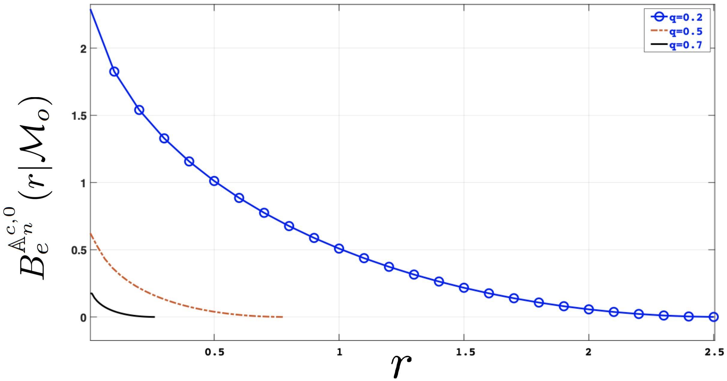
For the Hoeffding exponent $B_{e}^{\mathbb{A}^{c,0}}(r|\mathcal{M}_{o})$, finding a compact formula for the global maximum is not possible. However, numerical simulation guarantees that $B_{e}^{\mathbb{A}^{c,0}}(r|\mathcal{M}_{o})$ is a convex function that the first derivative has a unique zero. We solved the optimization numerically for depolarizing channel with three different parameters, see Fig. 7. $\square$

Example 31 (Pauli channel).

Let $\vec{p}=(p_{I},p_{x},p_{y},p_{z})$ be a probability vector. The Pauli channel is defined as follows:

$$\mathcal{P}_{\vec{p}}:\rho\mapsto p_{I}\rho+\sum_{i=x,y,z}p_{i}\sigma_{i}\rho\sigma_{i}^{\dagger},$$

that is, it returns the state with probability $p_{I}$ or applies the Pauli operators $\sigma_{x},\sigma_{y},\sigma_{z}$ with probabilities $p_{x},p_{y},p_{z}$, respectively.

For this channel, it can be seen by some algebra that (see e.g. (Hayashi:book, , Sec. 5.3) and PhysRevA.59.3290 )

$$\vec{t}=\begin{pmatrix}0\\ 0\\ 0\end{pmatrix}\quad\text{and}\quad T=\begin{pmatrix}p_{I}+p_{x}-p_{y}-p_{z}&0&0\\ 0&p_{I}-p_{x}+p_{y}-p_{z}&0\\ 0&0&p_{I}-p_{x}-p_{y}+p_{z}\\ \end{pmatrix}.$$ (53)

Therefore, the states on the surface of the Bloch sphere are mapped into the surface of the following ellipsoid:

$$\left(\frac{r_{x}}{p_{I}+p_{X}-p_{Y}-p_{z}}\right)^{2}+\left(\frac{r_{y}}{p_{I}-p_{X}+p_{Y}-p_{z}}\right)^{2}+\left(\frac{r_{z}}{p_{I}-p_{X}-p_{Y}+p_{z}}\right)^{2}=1.$$ (54)

Note that the Pauli channel shrinks the unit sphere with different magnitudes along each axis, and the two states on the surface of the ellipsoid that have the largest distance depends on the lengths of the coordinates on each axis. We need to choose the states along the axis that is shrunk the least. We define the following:

$$p_{\max}=\max\bigl{\{}|p_{I}+p_{X}-p_{Y}-p_{Z}|,|p_{I}-p_{X}+p_{Y}-p_{Z}|,|p_{I}-p_{X}-p_{Y}+p_{Z}|\bigr{\}},$$ (55)

then from the symmetry of the problem and the fact that the eigenvalues of the state $\vec{r}=(r_{x},r_{y},r_{z})$ are $\left\{\frac{1-|\vec{r}|}{2},\frac{1+|\vec{r}|}{2}\right\}$, the following can be seen after some algebra:

$$\sup_{\rho,\sigma}D_{\alpha}(\mathcal{M}_{o}(\rho)\|\mathcal{M}_{o}(\sigma))=\frac{1}{\alpha-1}\log Q(1-p_{\max},\alpha).$$ (56)

From this, for $0\leq r\leq-p_{\max}\log\frac{1-p_{\max}}{1+p_{\max}}$ and $p_{\max}\log\frac{1-p_{\max}}{1+p_{\max}}\leq a-b\leq-p_{\max}\log\frac{1-p_{\max}}{1+p_{\max}}$, we have

$$C^{\mathbb{A}^{c,0}}(a,b|\mathcal{M}) =\sup_{0\leq\alpha\leq 1}-\log Q(1-p_{\max},\alpha)-\alpha a-(1-\alpha)b,$$

$$B_{e}^{\mathbb{A}^{c,0}}(r|\mathcal{M}) =\sup_{0\leq\alpha\leq 1}\frac{\alpha-1}{\alpha}\left(r-\frac{1}{\alpha-1}\log Q(1-p_{\max},\alpha)\right).$$

Similar to our findings in Example 30, we can show that the generalized Hoeffding bound is maximized at

$$\alpha=\frac{1}{2}-\frac{\log\frac{\log\frac{1-p_{\text{max}}}{1+p_{\text{max}}}+(a-b)}{\log\frac{1-p_{\text{max}}}{1+p_{\text{max}}}-(a-b)}}{2\log\frac{1-p_{\text{max}}}{1+p_{\text{max}}}},$$

and this point is unique. The same conclusion using numerical optimization indicates that the Hoeffding bound of the Pauli channel resembles that of the depolarizing channel. Note that a depolarizing channel with parameter $q$ is equivalent to a Pauli channel with parameters $\left\{p_{I}=1-\frac{3q}{4},p_{x}=\frac{q}{4},p_{y}=\frac{q}{4},p_{z}=\frac{q}{4}\right\}$ (Hayashi:book, , Ex. 5.3). $\square$

Example 32 (Amplitude damping channel).

The amplitude damping channel with parameter $0\leq\gamma\leq 1$ is defined as follows:

$$\mathcal{A}_{\gamma}:\rho\mapsto A_{0}\rho A_{0}^{\dagger}+A_{1}\rho A_{1}^{\dagger},$$ (57)

where the Kraus operators are given as $A_{0}=\sqrt{\gamma}\outerproduct{0}{1}$ and $A_{1}=\outerproduct{0}{0}+\sqrt{1-\gamma}\outerproduct{1}{1}$.

Figure 8: The Bloch sphere and its image under the amplitude damping channel with parameter $\gamma$. There are two large and one small principal axes. As indicated in the right-hand figure, the points $(0,0,1)$ and $(0,0,2\gamma-1)$ are the intersection points of the surface of the displaced ellipsoid with the $z$ axis; the former point also is its intersection point with the Bloch sphere.

For this channel, simple algebra shows that

$$\vec{t}=\begin{pmatrix}0\\ 0\\ \gamma\end{pmatrix}\quad\text{and}\quad T=\begin{pmatrix}\sqrt{1-\gamma}&0&0\\ 0&\sqrt{1-\gamma}&0\\ 0&0&1-\gamma\\ \end{pmatrix}.$$ (58)

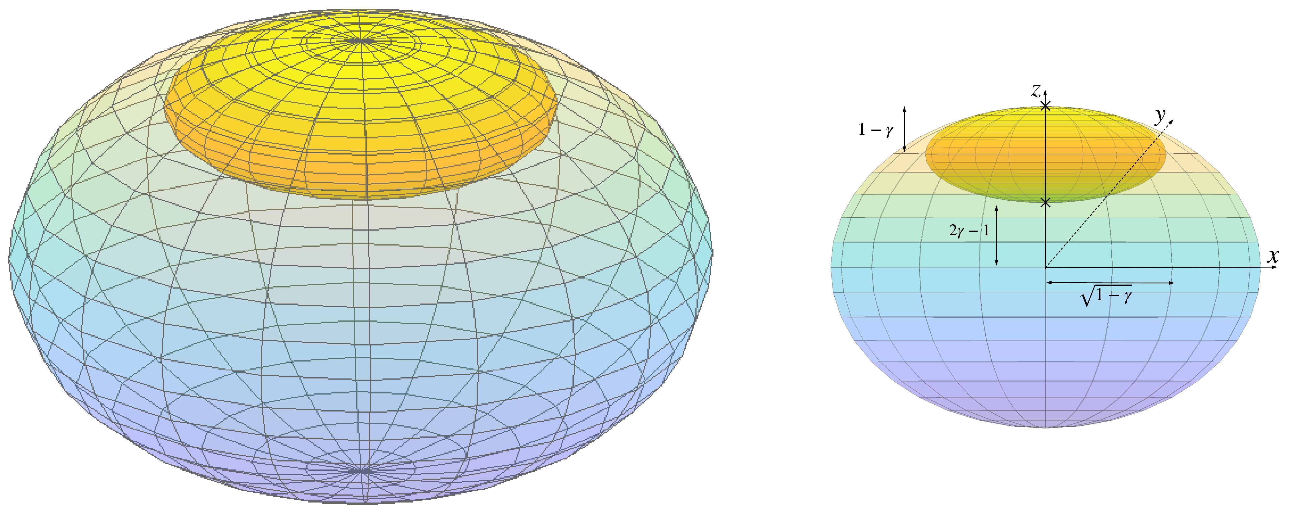
Note that unlike depolarizing and Pauli channels, $\vec{t}$ has a non-zero element for the amplitude damping channel, meaning that the amplitude damping channel is not unital. The non-zero $\vec{t}$ indicates shifting the center of the ellipsoid. The ellipsoid of output states of the amplitude damping channel is depicted in Fig. 8. Some algebra reveals the equation of the image to be as follows:

$$\left(\frac{r_{x}}{\sqrt{1-\gamma}}\right)^{2}+\left(\frac{r_{y}}{\sqrt{1-\gamma}}\right)^{2}+\left(\frac{r_{z}-\gamma}{1-\gamma}\right)^{2}=1.$$ (59)

To calculate the divergence, from the argument we made in Remark 29, we choose the optimal states on $x-z$ plane as $\vec{r}_{1}=(\sqrt{1-\gamma},0,\gamma)$ and $\vec{r}_{2}=(-\sqrt{1-\gamma},0,\gamma)$. It can be numerically checked that these points lead to maximum divergence. These two points correspond to the following states, respectively:

$$\rho_{1}=\frac{1}{2}\begin{pmatrix}1+\gamma&\sqrt{1-\gamma}\\ \sqrt{1-\gamma}&1-\gamma\\ \end{pmatrix}\quad\text{and}\quad\rho_{2}=\frac{1}{2}\begin{pmatrix}1+\gamma&-\sqrt{1-\gamma}\\ -\sqrt{1-\gamma}&1-\gamma\\ \end{pmatrix}.$$

Since $|\vec{r}_{1}|=|\vec{r}_{2}|=\sqrt{\gamma^{2}-\gamma+1}$, both states have the following eigenvalues:

$$\lambda_{1},\lambda_{2}=\frac{1\pm\sqrt{\gamma^{2}-\gamma+1}}{2},$$

and since $\rho_{1}$ and $\rho_{2}$ obviously do not commute, we find the eigenvectors for $\rho_{1}$ and $\rho_{2}$ respectively as follows:

$$\ket{\nu_{1}}=\frac{1}{\sqrt{1+(\frac{2\lambda_{1}-1-\gamma}{\sqrt{1-\gamma}})^{2}}}\begin{pmatrix}1\\ \frac{2\lambda_{1}-1-\gamma}{\sqrt{1-\gamma}}\\ \end{pmatrix},\quad\ket{\nu_{2}}=\frac{1}{\sqrt{1+(\frac{2\lambda_{2}-1-\gamma}{\sqrt{1-\gamma}})^{2}}}\begin{pmatrix}1\\ \frac{2\lambda_{2}-1-\gamma}{\sqrt{1-\gamma}}\\ \end{pmatrix},$$

and

$$\ket{\mu_{1}}=\frac{1}{\sqrt{1+(\frac{2\lambda_{1}-1-\gamma}{\sqrt{1-\gamma}})^{2}}}\begin{pmatrix}1\\ -\frac{2\lambda_{1}-1-\gamma}{\sqrt{1-\gamma}}\\ \end{pmatrix},\quad\ket{\mu_{2}}=\frac{1}{\sqrt{1+(\frac{2\lambda_{2}-1-\gamma}{\sqrt{1-\gamma}})^{2}}}\begin{pmatrix}1\\ -\frac{2\lambda_{2}-1-\gamma}{\sqrt{1-\gamma}}\\ \end{pmatrix}.$$

The following can be seen after some algebra:

$$\sup_{\rho,\sigma}D_{\alpha}(\mathcal{M}_{o}(\rho)\|\mathcal{M}_{o}(\sigma))=\frac{1}{\alpha-1}\log W(\gamma,\alpha),$$

where

$$W(\gamma,\alpha) =\lambda_{1}\left(\frac{1-\left(\frac{2\lambda_{1}-1-\gamma}{\sqrt{1-\gamma}}\right)^{2}}{1+\left(\frac{2\lambda_{1}-1-\gamma}{\sqrt{1-\gamma}}\right)^{2}}\right)^{2}+\lambda_{2}\left(\frac{1-\left(\frac{2\lambda_{2}-1-\gamma}{\sqrt{1-\gamma}}\right)^{2}}{1+\left(\frac{2\lambda_{2}-1-\gamma}{\sqrt{1-\gamma}}\right)^{2}}\right)^{2}$$

$$\phantom{==}+\frac{\left(Q(1-\sqrt{\gamma^{2}-\gamma+1},\alpha)\right)\left(1-\frac{(2\lambda_{1}-1-\gamma)(2\lambda_{2}-1-\gamma)}{(\sqrt{1-\gamma})^{2}}\right)^{2}}{\left(1+\left(\frac{2\lambda_{1}-1-\gamma}{\sqrt{1-\gamma}}\right)^{2}\right)\left(1+\left(\frac{2\lambda_{2}-1-\gamma}{\sqrt{1-\gamma}}\right)^{2}\right)}.$$

We also have

$$D(\mathcal{M}) =\lambda_{1}\log\lambda_{1}+\lambda_{2}\log\lambda_{2}-\lambda_{1}\log\lambda_{1}\left(\frac{1-\left(\frac{2\lambda_{1}-1-\gamma}{\sqrt{1-\gamma}}\right)^{2}}{1+\left(\frac{2\lambda_{1}-1-\gamma}{\sqrt{1-\gamma}}\right)^{2}}\right)^{2}-\lambda_{2}\log\lambda_{2}\left(\frac{1-\left(\frac{2\lambda_{2}-1-\gamma}{\sqrt{1-\gamma}}\right)^{2}}{1+\left(\frac{2\lambda_{2}-1-\gamma}{\sqrt{1-\gamma}}\right)^{2}}\right)^{2}$$

$$\phantom{=============}-\frac{(\lambda_{1}\log\lambda_{2}+\lambda_{2}\log\lambda_{1})\left(1-\frac{(2\lambda_{1}-1-\gamma)(2\lambda_{2}-1-\gamma)}{1-\gamma}\right)^{2}}{\left(1+\left(\frac{2\lambda_{1}-1-\gamma}{\sqrt{1-\gamma}}\right)^{2}\right)\left(1+\left(\frac{2\lambda_{2}-1-\gamma}{\sqrt{1-\gamma}}\right)^{2}\right)}.$$

Figure 9: Hoeffding exponent for amplitude damping channel when entangled inputs are not allowed. The legitimate values of $r$ for each exponent are imposed by the strong Stein’s lemma and differ as a function of $\gamma$, i.e. $D(\mathcal{M})$.

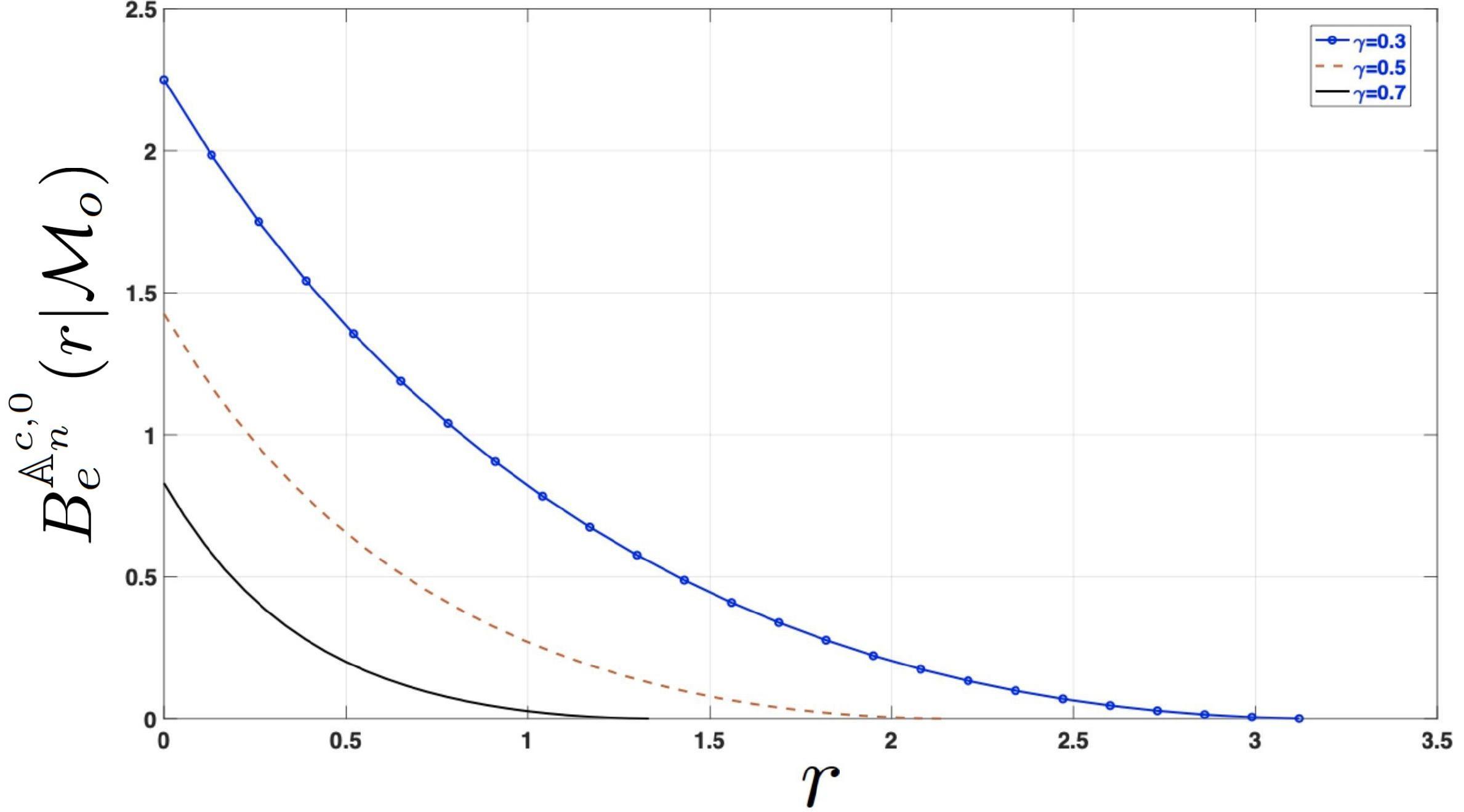
The cumbersome expressions reflect the complexity of analytically solving the optimizations; however, it can be seen numerically that the first derivative of the generalized Chernoff bound has a unique zero and its second derivative is positive ensuring the convexity. We calculate and plot the Hoeffding exponent for three different parameters of the amplitude damping channel in Fig. 9. $\square$

VIII Conclusion

In an attempt to further extend the classical results of 5165184 to quantum channels, we have shown that for the discrimination of a pair of cq-channels, adaptive strategies cannot offer any advantage over non-adaptive strategies concerning the asymmetric Hoeffding and the symmetric Chernoff problems in the asymptotic limit of error exponents, even when the input system is continuous. Our approach consists in associating to the cq-channels a pair of classical channels. This latter finding led us to prove the optimality of non-adaptive strategies for discriminating qq-channels via a subclass of protocols which only use classical feed-forward and product inputs.

In contrast, the most general strategy for discriminating qq-channels allows quantum feed-forward and entangled inputs. In this class, we have obtained two results for a pair of two entanglement-breaking channels. When these two entanglement-breaking channels are constructed via the same PVM, the most general strategy cannot improve the parallel scheme concerning the asymmetric Hoeffding and the symmetric Chernoff problems. In contrast, in an example of a pair of entanglement-breaking channels that are constructed via different PVMs, and in another example of a pair of qc-channels implementing general POVMs, we have shown asymptotic separations between the Chernoff and Hoeffding exponents of adaptive and non-adaptive strategies. These examples show the importance of the above condition for two entanglement-breaking channels. For general pairs of qq-channels, we leave open the question of the condition for the optimality of non-adaptive protocols; note that it is open already for entanglement-breaking channels.

We have also studied the hypothesis testing of binary information via a noisy quantum channel and have shown that when no entangled inputs nor quantum feedback are allowed, non-adaptive strategies are optimal. In addition, when the channel is an entanglement-breaking channel composed of a PVM followed by a state preparation, we have shown the optimality of non-adaptive strategies without the need for entangled inputs among all adaptive strategies.

References

- [1] Hsin-Yuan Huang, Richard Kueng, and John Preskill. Information-theoretic bounds on quantum advantage in machine learning. Phys. Rev. Lett., 126:190505, May 2021.
- [2] Dennis Kretschmann and Reinhard F. Werner. Quantum channels with memory. Physical Review A, 72(6):062323, Dec 2005.
- [3] Gus Gutoski and John Watrous. Toward a general theory of quantum games. In Proc. 39th annual ACM Symposium on Theory of Computing (STOC), pages 565–574, 2007.
- [4] Giulio Chiribella, G. Mauro D’Ariano, and Paolo Perinotti. Memory effects in quantum channel discrimination. Physical Review Letters, 101:180501, Oct 2008.
- [5] Giulio Chiribella, G. Mauro D’Ariano, and Paolo Perinotti. Transforming quantum operations: Quantum supermaps. Europhysics Letters, 83:30004, Aug 2008.
- [6] Giulio Chiribella, G. Mauro D’Ariano, and Paolo Perinotti. Theoretical framework for quantum networks. Physical Review A, 80:022339, Aug 2009.
- [7] Masahito Hayashi. Discrimination of Two Channels by Adaptive Methods and Its Application to Quantum System. IEEE Transactions on Information Theory, 55(8):3807–3820, Aug 2009.
- [8] John Watrous. Semidefinite Programs for Completely Bounded Norms. Theory of Computing, 5(11):217–238, Nov 2009.
- [9] Gus Gutoski. On a measure of distance for quantum strategies. Journal of Mathematical Physics, 53(3):032202, Mar 2012.
- [10] Stefano Pirandola, Bhaskar Roy Bardhan, Tobias Gehring, Christian Weedbrook, and Seth Lloyd. Advances in photonic quantum sensing. Nature Photonics, 12:724–733, Nov 2018. arXiv[quant-ph]:1811.01969.
- [11] Vishal Kataryia and Mark M. Wilde. Geometric distinguishability measures limit quantum channel estimation and discrimination. arXiv[quant-ph]:2004.10708, 2020.
- [12] Herman Chernoff. A measure of asymptotic efficiency for tests of a hypothesis based on the sum of observations. The Annals of Mathematical Statistics, 23(4):493–507, Dec 1952.
- [13] Wassily Hoeffding. Asymptotically optimal tests for multinomial distributions. The Annals of Mathematical Statistics, 36(2):369–401, Apr 1965.
- [14] Te Sun Han and Kingo Kobayashi. The strong converse theorem for hypothesis testing. IEEE Transactions on Information Theory, 35(1):178–180, Jan 1989.
- [15] Fumio Hiai and Dénes Petz. The proper formula for relative entropy and its asymptotics in quantum probability. Communications in Mathematical Physics, 143(1):99–114, 1991.
- [16] Tomohiro Ogawa and Hiroshi Nagaoka. Strong converse and Stein’s lemma in quantum hypothesis testing. IEEE Transactions on Information Theory, 46(7):2428–2433, Nov 2000.
- [17] Michael Nussbaum and Arleta Szkoła. The Chernoff lower bound for symmetric quantum hypothesis testing. The Annals of Statistics, 37(2):1040–1057, Apr 2009.
- [18] Koenraad M. R. Audenaert, John Calsamiglia, Ramon Muñoz-Tapia, Emili Bagan, Lluis Masanes, Antonio Acin, and Frank Verstraete. Discriminating States: The Quantum Chernoff Bound. Physical Review Letters, 98(16):160501, Apr 2007.
- [19] Masahito Hayashi. Quantum Information Theory: Mathematical Foundation. Springer Verlag, 2nd edition, 2016.
- [20] Tomohiro Ogawa and Masahito Hayashi. On error exponents in quantum hypothesis testing. IEEE Transactions on Information Theory, 50(6):1368–1372, June 2004.
- [21] Masahito Hayashi. Error exponent in asymmetric quantum hypothesis testing and its application to classical-quantum channel coding. Physical Review A, 76(6), Dec 2007.
- [22] Hiroshi Nagaoka. The Converse Part of The Theorem for Quantum Hoeffding Bound. arXiv:quant-ph/0611289, Nov 2006.
- [23] Aram W. Harrow, Avinatan Hassidim, Debbie W. Leung, and John Watrous. Adaptive versus nonadaptive strategies for quantum channel discrimination. Physical Review A, 81:032339, Mar 2010.
- [24] Aleksandra Krawiec, Łukasz Pawela, and Zbigniew Puchała. Discrimination of POVMs with rank-one effects. arXiv[quant-ph]:2002.05452, Feb 2020.
- [25] Mark M. Wilde, Mario Berta, Christoph Hirche, and Eneet Kaur. Amortized channel divergence for asymptotic quantum channel discrimination. Letters in Mathematical Physics, 110(8):2277–2336, 2020.
- [26] Mario Berta, Christoph Hirche, Eneet Kaur, and Mark M. Wilde. Stein’s lemma for classical-quantum channels. In 2019 IEEE International Symposium on Information Theory (ISIT), pages 2564–2568, 2019.
- [27] Zbigniew Puchała, Łukasz Pawela, Aleksandra Krawiec, Ryszard Kukulski, and Michał Oszmaniec. Multiple-shot and unambiguous discrimination of von Neumann measurements. arXiv[quant-ph]:1810.05122v3, Apr 2020.
- [28] Paulina Lewandowska, Aleksandra Krawiec, Ryszard Kukulski, Łukasz Pawela, and Zbigniew Puchała. Certification of quantum measurements. arXiv[quant-ph]:2009.06776, Sep 2020.
- [29] Stefano Pirandola and Cosmo Lupo. Ultimate Precision of Adaptive Noise Estimation. Physical Review Letters, 118:100502, Mar 2017. arXiv[quant-ph]:1609.02160.
- [30] Runyao Duan, Yuan Feng, and Mingsheng Ying. Perfect Distinguishability of Quantum Operations. Physical Review Letters, 103:210501, Nov 2009.
- [31] Runyao Duan, Chen Guo, Chi-Kwong Li, and Yinan Li. Parallel distinguishability of quantum operations. In 2016 IEEE International Symposium on Information Theory (ISIT), pages 2259–2263, July 2016.
- [32] Daniel Puzzuoli and John Watrous. Ancilla Dimension in Quantum Channel Discrimination. Annales Henri Poincaré, 18(4):1153–1184, 2017.
- [33] Xin Wang and Mark M. Wilde. Resource theory of asymmetric distinguishability for quantum channels. Physical Review Research, 1:033169, Dec 2019.
- [34] Kun Fang, Omar Fawzi, Renato Renner, and David Sutter. A chain rule for the quantum relative entropy. arXiv[quant-ph]:1909.05826, Sep 2019.
- [35] Tom Cooney, Milán Mosonyi, and Mark M. Wilde. Strong Converse Exponents for a Quantum Channel Discrimination Problem and Quantum-Feedback-Assisted Communication. Communications in Mathematical Physics, 344(3):797–829, June 2016.
- [36] Christoph Hirche, Masahito Hayashi, Emilio Bagan, and John Calsamiglia. Discrimination Power of a Quantum Detector. Physical Review Letters, 118(16):160502, 2017.
- [37] Alexei Kitaev. Quantum computations: algorithms and error correction. Russian Mathematical Surveys 52:6 1191-1249, 52(6):1191–1249, 1997.
- [38] Dorit Aharonov, Alexei Kitaev, and Noam Nisan. Quantum circuits with mixed states. In Proc.13th Annual ACM Symposium on Theory of Computation (STOC), pages 20–30, 1997.
- [39] Vern I. Paulsen. Completely Bounded Maps and Operator Algebras. Cambridge Studies in Advanced Mathematics. Cambridge University Press, 2002.
- [40] Nengkun Yu and Li Zhou. Chernoff Bound for Quantum Operations is Faithful. arXiv[quant-ph]:1705.01642, May 2017.
- [41] Stefano Pirandola, Riccardo Laurenza, Cosmo Lupo, and Jason L. Pereira. Fundamental limits to quantum channel discrimination. npj Quantum Information, 5:50, June 2019. arXiv[quant-ph]:1803.02834.
- [42] Christopher A. Fuchs and Jeroen van de Graaf. Cryptographic distinguishability measures for quantum-mechanical states. IEEE Transactions on Information Theory, 45(4):1216–1227, 1999.
- [43] Mark A. Naimark (Neumark). On a representation of additive operator set functions. Doklady Akademii Nauk SSSR – Comptes Rendus de l’Académie des Sciences de l’URSS (N.S.), 41(9):359–361, 1943.
- [44] Tomohiro Ogawa and Masahito Hayashi. On Error Exponents in Quantum Hypothesis Testing. arXiv:quant-ph/0206151, June 2002.
- [45] Constantin P. Niculescu and Lars-Erik Persson. Convex Functions and Their Applications. Springer Verlag, 2nd edition, 2018.
- [46] Christopher King and Mary-Beth Ruskai. Minimal entropy of states emerging from noisy quantum channels. IEEE Transactions on Information Theory, 47(1):192–209, 2001.
- [47] Akio Fujiwara and Paul Algoet. One-to-one parametrization of quantum channels. Physical Review A, 59(5):3290–3294, May 1999.