Benchmarking magnetizabilities with recent density functionals

Abstract

We have assessed the accuracy for magnetic properties of a set of 51 density functional approximations, including both recently published as well as already established functionals. The accuracy assessment considers a series of 27 small molecules and is based on comparing the predicted magnetizabilities to literature reference values calculated using coupled cluster theory with full singles and doubles and perturbative triples [CCSD(T)] employing large basis sets. The most accurate magnetizabilities, defined as the smallest mean absolute error, were obtained with the BHandHLYP functional. Three of the six studied Berkeley functionals and the three range-separated Florida functionals also yield accurate magnetizabilities. Also some older functionals like CAM-B3LYP, KT1, BHLYP (BHandH), B3LYP and PBE0 perform rather well. In contrast, unsatisfactory performance was generally obtained with Minnesota functionals, which are therefore not recommended for calculations of magnetically induced current density susceptibilities, and related magnetic properties such as magnetizabilities and nuclear magnetic shieldings.

We also demonstrate that magnetizabilities can be calculated by numerical integration of the magnetizability density; we have implemented this approach as a new feature in the gauge-including magnetically induced current method (Gimic). Magnetizabilities can be calculated from magnetically induced current density susceptibilities within this approach even when analytical approaches for magnetizabilities as the second derivative of the energy have not been implemented. The magnetizability density can also be visualized, providing additional information that is not otherwise easily accessible on the spatial origin of the magnetizabilities.

Molecular Sciences Software Institute, Blacksburg, Virginia 24061, United States NMR,GIMIC

1 Introduction

Computational methods based on density-functional theory (DFT) are commonly used in quantum chemistry, because DFT calculations are rather accurate despite their relatively modest computational costs. Older functionals such as the Becke’88–Perdew’86^{1, 2} (BP86), Becke’88–Lee–Yang–Parr^{1, 3} (BLYP) and Perdew–Burke–Ernzerhof^{4, 5} (PBE) functionals at the generalized gradient approximation (GGA) as well as the B3LYP⁶ and PBE0^{7, 8} hybrid functionals are still often employed, even though newer functionals with improved accuracy for energies and electronic properties have been developed.

The accuracy and reliability of various density functional approximations (DFAs) has been assessed in a huge number of applications and benchmark studies.^{9, 10, 11, 12, 13, 14, 15, 16, 17} It is important to note that functionals that are accurate for energetics may be less suited for calculations of other molecular properties.¹⁶ In specific, the accuracy of magnetic properties calculated within DFAs has been benchmarked by comparing magnetizabilities and nuclear magnetic shieldings to those obtained from coupled-cluster calculations using large basis sets,^{18, 19} although modern DFAs have been less systematically investigated.^{20, 21, 22, 23, 16} The same also holds for nuclear independent chemical shifts^{24, 25, 26, 27, 28} and magnetically induced current density susceptibilities,^{29, 30, 31, 32, 33, 34, 35, 36} which have been studied for a large number of molecules, but whose accuracy has never been benchmarked properly.

Magnetizabilities are usually calculated as the second derivative of the electronic energy with respect to the external magnetic perturbation,^{37, 38, 39, 40, 41}

$$\xi_{\alpha\beta}=-\frac{\partial^{2}E}{\partial B_{\alpha}\partial B_{\beta}}\Bigg{|}_{{\bf B}={\bf 0}}.$$ (1)

Such analytic implementations for magnetizabilities exist in several quantum chemistry programs. However, since the magnetic interaction energy in (LABEL:Emag) can also be written as an integral over the magnetic interaction energy density $\rho^{\bf B}({\bf r})$ that is given by the scalar product of the magnetically induced current density $\mathbf{J^{B}}(\mathbf{r})$ with the vector potential $\mathbf{A^{B}}(\mathbf{r})$ of the external magnetic field $\mathbf{B}$^{42, 43, 44, 45, 30, 31}

$$E=\int\rho^{\bf B}({\bf r})~{}\mathrm{d}^{3}r=-\frac{1}{2}\int\mathbf{A}^{\mathbf{B}}(\mathbf{r})\cdot\mathbf{J^{B}}(\mathbf{r})~{}\mathrm{d}^{3}r,$$ (2)

an approach based on quadrature is also possible. As will be seen in theory, the numerical integration approach for the magnetizability provides additional information about its spatial origin that is not available with the analytic approach based on second derivatives: the tensor components of the magnetizability density defined in theory are scalar functions that can be visualized, and the integration approach can be used to provide detailed information about the origin of the corresponding components of the magnetizability tensor. Similar approaches have been used in the literature for studying spatial contributions to nuclear magnetic shielding constants.^{46, 47, 48, 49, 50, 51, 52, 53}

We will describe our methods for numerical integration of magnetizabilities using the current density susceptibility in theory, implementation. Then, in methods, we will list the studied set of density functionals, and present the results in results: the functional benchmark is discussed in benchmark, and magnetizability densities and spatial contributions to magnetizabilities are analyzed in magnetizability. The conclusions of the study are summarized in conclusions. Atomic units are used throughout the text, unless stated otherwise, and summation over repeated indices is assumed.

2 Theory

The current density $\mathbf{J^{B}}(\mathbf{r})$ in (LABEL:Emag) is formally defined as the real part $(\mathcal{R})$ of the mechanical momentum density,

$$\mathbf{J}^{\mathbf{B}}(\mathbf{r})=-\mathcal{R}\left[\Psi^{*}(\mathbf{r})\left(\mathbf{p}-\mathbf{A}^{\mathbf{B}}(\mathbf{r})\right)\Psi(\mathbf{r})\right],$$ (3)

where $\mathbf{p}=-\mathrm{i}\nabla$ is the momentum operator. Substituting (LABEL:Emag) into (LABEL:zeta-secondder) straightforwardly leads to

$$\xi_{\alpha\beta}=\frac{\partial^{2}}{\partial B_{\alpha}\partial B_{\beta}}\frac{1}{2}\int\mathbf{A}^{\mathbf{B}}(\mathbf{r})\cdot\mathbf{J^{B}}(\mathbf{r})~{}\mathrm{d}^{3}r\Bigg{|}_{{\bf B}={\bf 0}}.$$ (4)

The current density susceptibility tensor^{29, 30, 31} (CDT) is defined as the first derivative of the magnetically induced current density with respect to the components of the external magnetic field in the limit of a vanishing magnetic field,^{32, 33, 34, 35}

$${\cal J}^{B_{\beta}}_{\gamma}=\frac{\partial J_{\gamma}^{\bf B}}{\partial B_{\beta}}\Bigg{|}_{{\bf B}={\bf 0}}.$$ (5)

The vector potential $\mathbf{A}^{\mathbf{B}}(\mathbf{r})$ of an external static homogeneous magnetic field is expressed as

$$\mathbf{A}^{\mathbf{B}}(\mathbf{r})=\frac{1}{2}\mathbf{B}\times(\mathbf{r}-\mathbf{R}_{O}),$$ (6)

where $\mathbf{R}_{O}$ is the chosen gauge origin. The $\alpha\beta$ component of the magnetizability tensor can then be obtained from (LABEL:magnetizability,_MCDSS,_vecpot) as

$$\xi_{\alpha\beta}=\int\rho_{\alpha\beta}^{\xi}(\mathbf{r})\mathrm{d}^{3}r,$$ (7)

where the magnetizability density is defined as

$$\rho_{\alpha\beta}^{\xi}({\bf r})=\frac{1}{2}\sum_{\delta\gamma}\epsilon_{\alpha\delta\gamma}{r}_{\delta}{\cal J}^{B_{\beta}}_{\gamma}(\mathbf{r})$$ (8)

where $\epsilon_{\alpha\delta\gamma}$ is the Levi–Civita symbol, $\alpha$, $\beta$, $\gamma$, and $\delta$ are one of the Cartesian directions $(x,y,z)$, and $r_{\delta}$ also denotes one of $(x,y,z)$. The components of the magnetizability density tensor $\rho^{\xi}_{\alpha\beta}({\bf r})$ are scalar functions that can be visualized to obtain information about the spatial contributions to the corresponding element of the magnetizability tensor $\xi_{\alpha\beta}$.

As the isotropic magnetizability ($\overline{\xi}$) is obtained as the average of the diagonal elements of the magnetizability tensor

$$\overline{\xi}=\frac{1}{3}\mathrm{Tr}~{}\xi=\int\overline{\rho}^{\xi}({\bf r})\mathrm{d}^{3}r,$$ (9)

we introduce the isotropic magnetizability density $\rho^{\overline{\xi}}({\bf r})$ defined as

$$\overline{\rho}^{\xi}({\bf r})=\frac{1}{3}\text{Tr}~{}\boldsymbol{\rho}^{\xi}({\bf r}),$$ (10)

which yields information about the spatial origin of the isotropic magnetizability, as we will demonstrate in magnetizability.

Although there is freedom with regard to the choice of the gauge origin of $\mathbf{A}^{\mathbf{B}}(\mathbf{r})$, the magnetic flux density $\mathbf{B}$ is uniquely defined via (LABEL:vecpot), because $\mathbf{B}=\nabla\times(\mathbf{A}(\mathbf{r})+\nabla f(\mathbf{r}))$ holds for any differentiable scalar function $f(\mathbf{r})$. The exact solution of the Schrödinger equation should also be gauge invariant. However, the use of finite one-particle basis sets introduces gauge dependence in quantum chemical calculations of magnetic properties. The CDT can be made gauge-origin independent by using gauge-including atomic orbitals (GIAOs), also known as London atomic orbitals (LAOs),^{54, 55, 32}

$$\chi_{\mu}(\mathbf{r})=e^{-\mathrm{i}(\mathbf{B}\times[\mathbf{R}_{\mu}-\mathbf{R}_{O}]\cdot\mathbf{r})/2}\chi_{\mu}^{(0)}\left(\mathbf{r}\right),$$ (11)

where $\mathrm{i}$ is the imaginary unit and $\chi_{\mu}^{(0)}(\mathbf{r})$ is a standard atomic-orbital basis function centered at $\mathbf{R}_{\mu}$. GIAOs eliminate the gauge origin from the expression used for calculating the CDT; the expression we use is given in the supporting information (SI). Since the expression for the magnetizability density in (LABEL:Biot-Savart,_magdens) can be computed by quadrature, magnetizabilities can be obtained from the CDT even if the corresponding analytical calculation of magnetizabilities as the second derivative of the energy has not been implemented.

3 Implementation

The present implementation is based on the Gimic program⁵⁶ and the Numgrid library,⁵⁷ which are both freely available open-source software. Gauge-independent CDTs can be calculated with Gimic^{32, 33, 34, 35} using the density matrix, the magnetically perturbed density matrices and information about the basis set.

In order to evaluate (LABEL:Biot-Savart), a molecular integration grid is first generated from atom-centered grids with the Numgrid library, as described by Becke ⁵⁸. In Numgrid, the grid weights are scaled according to the Becke partitioning scheme using a Becke hardness of 3;⁵⁸ the atom-centered grids are determined by a radial grid generated as suggested by Lindh et al. ⁵⁹, and angular grids due to Lebedev ⁶⁰ are used.

Given the quadrature grid, the diagonal elements of the magnetizability tensor are calculated in Gimic from the Cartesian coordinates of the $n$ grid points multiplied with the CDT calculated in the grid points. For example, the $\xi_{xx}$ element of the magnetizability tensor is obtained from (LABEL:Biot-Savart) as

$$\xi_{xx}=\sum_{i=1}^{n}\rho^{\xi}_{i;xx}$$ (12)

where the $xx$ component of the magnetizability density tensor at grid point $i$ is

$$\rho^{\xi}_{i;xx}=\frac{1}{2}\left[\left(y{\cal J}^{B_{x}}_{z}\right)_{i}-\left(z{\cal J}^{B_{x}}_{y}\right)_{i}\right]$$ (13)

where $\left(y{\cal J}^{B_{x}}_{z}\right)_{i}$ and $\left(z{\cal J}^{B_{x}}_{y}\right)_{i}$ are the product of the $z$ and $y$ components of the CDT calculated in grid point $i$ with the Cartesian coordinates $y$ and $z$ of the grid point, respectively, and the external magnetic field perturbation is along the $x$ axis, $B_{x}$. The $\xi_{yy}$ and $\xi_{zz}$ elements are obtained analogously.

4 Computational Methods

Calculations are performed for the set of 28 molecules studied in ref. 18 that also provides our molecular structures and the CCSD(T) reference values: AlF, C2H4, C3H4, CH2O, CH3F, CH4, CO, FCCH, FCN, H2C2O, H2O, H2S, H4C2O, HCN, HCP, HF, HFCO, HOF, LiF, LiH, N2, N2O, NH3, O3, OCS, OF2, PN, and SO2. However, as in ref. 18, O3 was omitted from the analysis, since it is an outlier, and due to the fact that the reliability of the CCSD(T) level of theory is not guaranteed for this system: the perturbative triples correction to the magnetizability of O3 is $-46.2\times 10^{-30}\,{\rm J}/{\rm T}^{2}$, indicating that the CCSD(T) result might still have large error bars.¹⁸ The results of this work thus only pertain to the 27 other molecules, as in ref. 18.

Table 1: Functionals at the local density approximation (LDA) and the generalized gradient approximation (GGA) considered in this work. GH stands for global hybrid and RS for range separated hybrid. The amount of Hartree–Fock (HF) exchange, or exact exchange in the short range (SR) and long range (LR) are also given.

Functional	Hybrid	Type	Notes	Libxc IDa	References
LDA		LDA		1+7	61, 62, 63
BLYP		GGA		106+131	1, 3, 64
BP86		GGA		106+132	1, 2
CHACHIYO		GGA		298+309	65, 66
KT1		GGA		167	67
KT2		GGA		146	67
KT3		GGA	PySCF data used	587	68
N12		GGA		82+80	69
PBE		GGA		101+130	4, 5
B3LYP	GH	GGA	20% HF	402	6
revB3LYPb	GH	GGA	20% HF	454	70
B97-2	GH	GGA	21% HF	410	71
B97-3	GH	GGA	26.9% HF	414	72
BHLYPc	GH	GGA	50% HF	435	61, 62, 73
BHandHLYPd	GH	GGA	50% HF	436	1, 73
PBE0	GH	GGA	25% HF	406	7, 8
QTP17	GH	GGA	62% HF	416	74
N12-SX	RS	GGA	25% SR, 0% LR	81+79	75
CAM-B3LYP	RS	GGA	19% SR, 65% LR	433	76
CAMh-B3LYPe	RS	GGA	19% SR, 50% LR	–	77
CAM-QTP-00	RS	GGA	54% SR, 91% LR	490	78
CAM-QTP-01	RS	GGA	23% SR, 100% LR	482	79
CAM-QTP-02	RS	GGA	28% SR, 100% LR	491	80
$\omega$B97	RS	GGA	0% SR, 100% LR	463	81
$\omega$B97X	RS	GGA	15.8% SR, 100% LR	464	81
$\omega$B97X-D	RS	GGA	22.2% SR, 100% LR	471	82
$\omega$B97X-V	RS	GGA	16.7% SR, 100% LR	531	83

• Two numbers indicate the exchange and the correlation functional respectively. A single number indicates an exchange-correlation functional.

• Revised version

• Following King el al. in refs. 84, 85, 86, BHLYP is defined as 50% LDA exchange, 50% of HF exchange, and 100% LYP correlation. It is sometimes also known as BHandH, which is its keyword in Gaussian.

• BHandHLYP is 50% Becke’88 exchange, 50% HF exchange, and 100% LYP correlation.

• CAMh-B3LYP is defined using the XCFun library with $\alpha=0.19;\beta=0.31;\mu=0.33$.

Table 2: Meta-GGA functionals (mGGA) considered in this work. The notation is the same as in ldas-ggas.

Functional	Hybrid	Type	Notes	Libxc IDa	References
B97M-V		mGGA		254	87
M06-L		mGGA		449+235	88
revM06-Lb		mGGA		293+294	89
M11-L		mGGA		226+75	90
MN12-L		mGGA		227+74	91
MN15-L		mGGA		268+269	92
TASK		mGGA		707+13	93, 94
MVS		mGGA		257+83	95, 96
SCAN		mGGA		263+267	97
rSCANc		mGGA		493+494	98
TPSS		mGGA		457	99, 100
revTPSSb		mGGA		212+241	96, 101
TPSSh	GH	mGGA	10% HF	457	102
revTPSShb	GH	mGGA	10% HF	458	96, 101, 102
M06	GH	mGGA	27% HF	449+235	103
revM06b	GH	mGGA	40.4% HF	305+306	104
M06-2X	GH	mGGA	54% HF	450+236	103
M08-HX	GH	mGGA	52.2% HF	295+78	105
M08-SO	GH	mGGA	56.8% HF	296+77	105
MN15	GH	mGGA	44% HF	268+269	106
M11	RS	mGGA	42.8% SR, 100% LR	297+76	107
revM11b	RS	mGGA	22.5% SR, 100% LR	304+172	108
MN12-SX	RS	mGGA	25% SR, 0% LR	248+73	75
$\omega$B97M-V	RS	mGGA	15% SR, 100% LR	531	109

• Two numbers indicate the exchange and the correlation functional respectively. A single number indicates an exchange-correlation functional.

• Revised version

• Regularized version

Electronic structure calculations were performed with Hartree–Fock (HF) and the functionals listed in ldas-ggas, mggas using Turbomole 7.5¹¹⁰. Several rungs of Jacob’s ladder were considered when choosing the functionals listed in ldas-ggas, mggas: local density approximations (LDA), generalized gradient approximations (GGAs), and meta-GGAs (mGGAs). Several kinds of functionals are also included: (pure) density functional approximations, global hybrid (GH) functionals with a constant amount of HF exchange, as well as range-separated (RS) hybrids with a given amount of HF exchange in the short range (SR) and the long range (LR). As can be seen in ldas-ggas, mggas, the evaluated functionals consist of one pure LDA, 8 pure GGAs, 8 global hybrid GGAs, 10 range-separated hybrid GGAs, 12 mGGAs, 8 global hybrid mGGAs, and 4 range-separated mGGAs, in addition to HF.

The Dunning aug-cc-pCVQZ basis set^{111, 112, 113, 114, 115} (with aug-cc-pVQZ on the hydrogen atoms) and benchmark quality integration grids were employed in all calculations. Universal auxiliary basis sets¹¹⁶ were used with the resolution-of-the-identity approximation for the Coulomb interaction in all Turbomole calculations. All density functionals were evaluated in Turbomole with Libxc,¹¹⁷ except the calculations with the recently published CAMh-B3LYP functional for which XCFun was used.¹¹⁸ Magnetizabilities were subsequently evaluated with Gimic by numerical integration of (LABEL:Biot-Savart). The data necessary for evaluating the CDT in Gimic were obtained from Turbomole calculations of nuclear magnetic resonance (NMR) shielding constants employing GIAOs.^{54, 55, 119, 110, 120}

Although response calculations are not possible at the moment in the presence of the non-local correlation kernel used in $\omega$B97X-V, B97M-V, and $\omega$B97M-V, we have estimated the importance of the van der Waals (vdW) effects on the magnetic properties by comparing magnetizabilities obtained with orbitals optimized with and without the vdW term in the case of SO2. The magnetizability obtained with the vdW optimized orbitals differed by only $0.4\times 10^{-30}\,{\rm J}/{\rm T}^{2}$ (0.14%) from that obtained from a calculation where the vdW term was omitted in the orbital optimization. Thus, the vdW term appears to have very little influence on magnetizabilities, as is already well-known in the literature for other properties.¹²¹ The vdW term was therefore not included in the calculations using the $\omega$B97X-V, B97M-V, and $\omega$B97M-V functionals in this study.

The accuracy of the numerical integration in Gimic was assessed by comparing the Turbomole/Gimic magnetizability data to analytical values from PySCF,¹²² in which Libxc¹¹⁷ was also used to evaluate the density functionals. Since PySCF does not currently support magnetizability calculations with mGGA functionals or range-separated functionals, further calculations were undertaken with Gaussian 16.¹²³. The analytical magnetizabilities from PySCF and Gaussian were found to be in perfect agreement for the studied LDA and GGA functionals available in both codes (LDA, BP86, PBE, PBE0, BLYP, B3LYP and BHLYP). Comparison of the data from PySCF to the Gimic data revealed the numerically integrated magnetizabilities to be accurate, as the magnetizabilities agreed within $0.5\times 10^{-30}\,{\rm J}/{\rm T}^{2}$ for all molecules using the B3LYP, B97-2, B97-3, BLYP, BP86, KT1, KT2, LDA, PBE, and PBE0 functionals; the small discrepancy may arise from use of the resolution-of-identity approximation¹²⁴ in Turbomole or from the numerical integration of the magnetizability density. A comparison of the raw data for BP86 and B3LYP is given in the SI.

The magnetizabilities calculated with Gaussian and Turbomole using the meta-GGA functionals were found to differ. The discrepancies between the magnetizabilities obtained with the two programs are due to the use of different approaches to handle the gauge invariance of the kinetic energy density in meta-GGAs, which are described in refs. 125 and 126 for Gaussian and Turbomole, respectively. We found the Turbomole data to be significantly closer to the CCSD(T) reference values.

Finally, since we found the implementation of the KT3 functional in Libxc version 5.0.0 used by Turbomole to be flawed, the KT3 results in this study are based on calculations with PySCF with a corrected version of Libxc.

5 Results

5.1 Functional benchmark

Table 3: The mean absolute errors (MAEs), mean errors (MEs), and standard deviations (STDs) for the magnetizabilities of the 27 studied molecules in units of $10^{-30}\,{\rm J}/{\rm T}^{2}$ from the CCSD(T) reference with the studied functionals. The functionals are ordered in increasing MAE.

Rank	Functional	MAE	ME	STD	Rank	Functional	MAE	ME	STD
1	BHandHLYP	3.11	2.15	4.65	27	revTPSSh	7.14	7.05	5.94
2	CAM-QTP-00	3.22	0.88	4.67	28	TPSSh	7.20	7.07	6.02
3	$\omega$B97X-V	3.22	2.51	4.36	29	B97-2	7.24	7.07	6.40
4	CAM-QTP-01	3.23	0.59	4.49	30	M08-HX	7.34	5.17	10.27
5	CAM-QTP-02	3.28	-0.23	4.36	31	BLYP	7.91	5.69	8.75
6	$\omega$B97	3.54	2.44	4.75	32	N12-SX	8.04	7.89	7.48
7	$\omega$B97M-V	3.61	0.41	4.75	33	revTPSS	8.20	7.86	6.68
8	CAM-B3LYP	3.73	2.38	4.86	34	TPSS	8.22	7.85	6.85
9	MN12-SX	3.80	0.22	5.34	35	revM11	8.23	6.83	10.03
10	CAMh-B3LYP	4.23	3.22	5.17	36	TASK	8.27	7.31	7.43
11	$\omega$B97X	4.25	3.71	5.22	37	BP86	8.59	7.30	8.75
12	QTP-17	4.58	3.77	5.45	38	M11-L	8.92	5.20	9.26
13	BHLYP	4.73	0.10	6.47	39	revM06	8.94	8.67	10.27
14	B97M-V	5.19	4.13	5.58	40	PBE	9.13	7.07	9.42
15	revB3LYP	5.45	4.34	6.13	41	KT3	9.19	8.38	8.08
16	B3LYP	5.47	4.72	5.97	42	LDA	9.55	5.37	11.36
17	MN12-L	5.79	-2.03	8.02	43	CHACHIYO	9.76	9.17	8.88
18	KT1	5.87	1.15	7.11	44	M11	9.93	7.61	13.77
19	rSCAN	5.91	5.00	6.06	45	M06-2X	10.15	9.01	13.12
20	PBE0	5.96	5.56	6.81	46	MVS	10.35	9.92	9.20
21	$\omega$B97X-D	6.22	5.89	6.35	47	M08-SO	10.40	8.09	14.34
22	SCAN	6.30	5.89	5.96	48	N12	10.89	10.01	9.58
23	KT2	6.42	5.58	7.21	49	MN15	11.45	10.45	12.82
24	MN15-L	6.57	-5.27	6.94	50	M06-L	12.49	12.45	9.42
25	B97-3	6.61	6.61	6.26	51	M06	13.34	13.11	13.16
26	revM06-L	7.00	6.23	5.98	52	HF	18.40	7.48	61.81

The deviations of the DFT magnetizabilities from the CCSD(T) reference values of ref. 18 are visualized as ideal normal distributions (NDs) in normal. The visualization shows the idealized distribution of the error in the magnetizability for each functional, based on the computed mean errors (ME) and standard deviation of the error (STD) given in errors. The raw data on the magnetizabilities and the differences from the CCSD(T) reference are available in the SI. Although the error distributions in normal are instructive, we will employ mean absolute errors (MAEs) in order to rank the functionals studied in this work in a simple, unambiguous fashion. The MAEs are also given in errors.

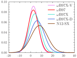
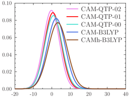
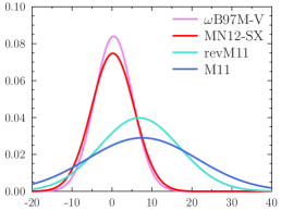
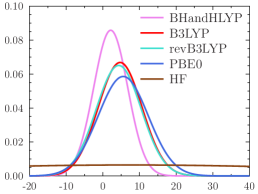
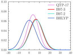
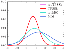
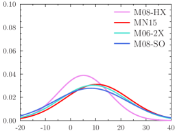
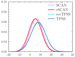
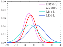
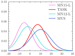
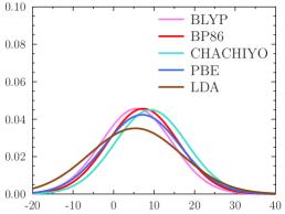
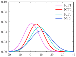
Figure 1: Normal distributions (ND) representing the errors in the magnetizabilities for the 27 benchmark reproduced by the studied functionals, obtained by plotting the data presented in errors. The curves are ordered in each figure by increasing standard deviation. The NDs of RS functionals are shown in figure1a, figure1b, figure1c. The NDs of the GH functionals are shown in figure1d, figure1e, figure1f, figure1g. The NDs of the mGGA functionals are shown in figure1h, figure1i, figure1j. The NDs of the LDA and GGA functionals are shown in figure1k, figure1l.

Examination of the data in errors shows that range-separated (RS) functionals generally yield accurate magnetizabilities. Judged by the mean absolute error, the best performance is obtained with the BHandHLYP GH functional. BHandHLYP is followed by 10 RS functionals, which have much sharper distributions than the rest of the studied functionals. The best performing RS functionals are three of the six Berkeley RS functionals ($\omega$B97X-V, $\omega$B97, $\omega$B97M-V) and the three RS functionals from the University of Florida’s Quantum Theory Project (QTP) CAM-QTP-00, CAM-QTP-01, and CAM-QTP-02. Five of these functionals have 100% long-range (LR) HF exchange, while the CAM-QTP-00 functional has 91% LR HF exchange. The two other RS Berkeley functionals with 100% LR exchange are ranked $11^{\mathrm{th}}$ ($\omega$B97X) and $21^{\mathrm{st}}$ ($\omega$B97X-D) among the studied functionals. The NDs of the studied RS GGA functionals are shown in figure1a, figure1b, whereas the NDs of the studied RS mGGA functionals are shown in figure1c.

The CAM-B3LYP (65% LR HF exchange) and CAMh-B3LYP (50% LR HF exchange) functionals are among the top ten functionals (ranked $8^{\mathrm{th}}$ and 10^th, respectively). CAM-B3LYP was designed for the accurate description of charge transfer excitations in a dipeptide model,⁷⁶ while CAMh-B3LYP functional is aimed at excitation energies of biochromophores.⁷⁷

The best Minnesota functional, MN12-SX, is ranked $9^{\mathrm{th}}$. MN12-SX is a highly parameterized functional with 58 parameters that is known to require the use of extremely accurate integration grids.¹³ Furthermore, since MN12-SX is a RS functional with HF exchange only in the short range (SR), it may have problems modeling magnetic properties of antiaromatic molecules sustaining strong ring currents in the paratropic (nonclassical) direction.^{127, 128, 129} We illustrate this with calculations on the strongly antiaromatic tetraoxa-isophlorin molecule in the Supporting Information: MN12-SX yields a magnetizability that is four times larger than the LMP2 [local second-order Møller–Plesset perturbation theory] reference value, while the magnetizabilities from BHandHLYP and CAM-B3LYP are in good agreement with LMP2. The N12-SX functional ranked $32^{\mathrm{nd}}$ is also a RS functional with 0% LR exchange. The RS Minnesota functionals with 100% LR HF exchange (M11 and revM11) have large MAEs of $9.93\times 10^{-30}\,{\rm J}/{\rm T}^{2}$ and $8.87\times 10^{-30}\,{\rm J}/{\rm T}^{2}$ and are ranked $44^{\mathrm{th}}$ and $35^{\mathrm{th}}$, respectively.

The best global hybrid (GH) functional is BHandHLYP, which is ranked $1^{\mathrm{st}}$ among all functionals of this study, as was already mentioned above. Among GHs, BHandHLYP is followed by QTP-17, which is ranked $12^{\mathrm{th}}$. Old and established GH functionals like BHLYP a.k.a. BHandH, B3LYP, and PBE0 perform almost as well as QTP-17 and are ranked $13^{\mathrm{th}}$, $16^{\mathrm{th}}$, and $20^{\mathrm{th}}$, respectively. The performance of revB3LYP is practically the same as for B3LYP; the same holds for revTPSSh and TPSSh. The other established GH functionals like B97-2, B97-3, TPSSh and newer ones like revTPSSh and M08-HX are found in the beginning of the second half of the ranking list, whereas M08-SO, M06, revM06, M06-2X, MN15, and M06 are ranked between $39^{\mathrm{th}}$ and $51^{\mathrm{st}}$. The NDs of the GH functionals are compared in figure1d, figure1e, figure1f, figure1g.

B97M-V, at the $14^{\mathrm{th}}$ place, is the best pure mGGA functional. The rSCAN and SCAN functionals are ranked $19^{\mathrm{th}}$ and $22^{\mathrm{th}}$, respectively, whereas revTPSS and TPSS appear at positions 33 and 34, respectively. The pure mGGA functionals of the Minnesota series are ranked $17^{\mathrm{th}}$ (MN12-L), $24^{\mathrm{th}}$ (MN15-L), $26^{\mathrm{th}}$ (revM06-L), and $50^{\mathrm{th}}$ (M06-L). The performance of the Minnesota pure mGGA functionals, excluding M06-L, is about the same as that of TASK and the other mGGA functionals. The magnetizabilities calculated with the revised M06-L (revM06-L) functional are more accurate than those with M06-L. The MVS mGGA functional is ranked $46^{\mathrm{th}}$. The NDs for the mGGA functionals are shown in figure1h, figure1i, figure1j.

The magnetizabilities calculated with several of the Minnesota functionals are inaccurate. Seven of the eight worst performing functionals (M11, M06-2X, MVS, M08-SO, N12, MN15, M06-L, M06) in errors are Minnesota functionals. Five other Minnesota functionals are also ranked in the lower half, placing $30^{\mathrm{th}}$ (M08-HX), $32^{\mathrm{th}}$ (N12-SX), $35^{\mathrm{th}}$ (revM11), $38^{\mathrm{th}}$ (M11-L), and $39^{\mathrm{th}}$ (revM06).

The KT1 and KT2 functionals are the best GGA functionals, ranking $18^{\mathrm{th}}$ and $23^{\mathrm{rd}}$, respectively; both KT1 and KT2 have been optimized for NMR shieldings.⁶⁷ The older commonly-used GGAs i.e., BLYP, BP86, and PBE are ranked $31^{\mathrm{st}}$, $37^{\mathrm{th}}$, and $40^{\mathrm{th}}$, respectively, which is only slightly better than KT3 ranked $41^{\mathrm{st}}$ and LDA ranked $42^{\mathrm{nd}}$. The CHACHIYO and N12 functionals, which are newer GGAs, are ranked $43^{\mathrm{rd}}$ and $48^{\mathrm{th}}$, respectively. The NDs of the GGA functionals and the LDA are shown in figure1k, figure1l.

The magnetizabilities calculated at the HF level are significantly less accurate and have a much larger MAE-STD than those obtained at the DFT levels, and we cannot recommend the use of HF for magnetic properties.

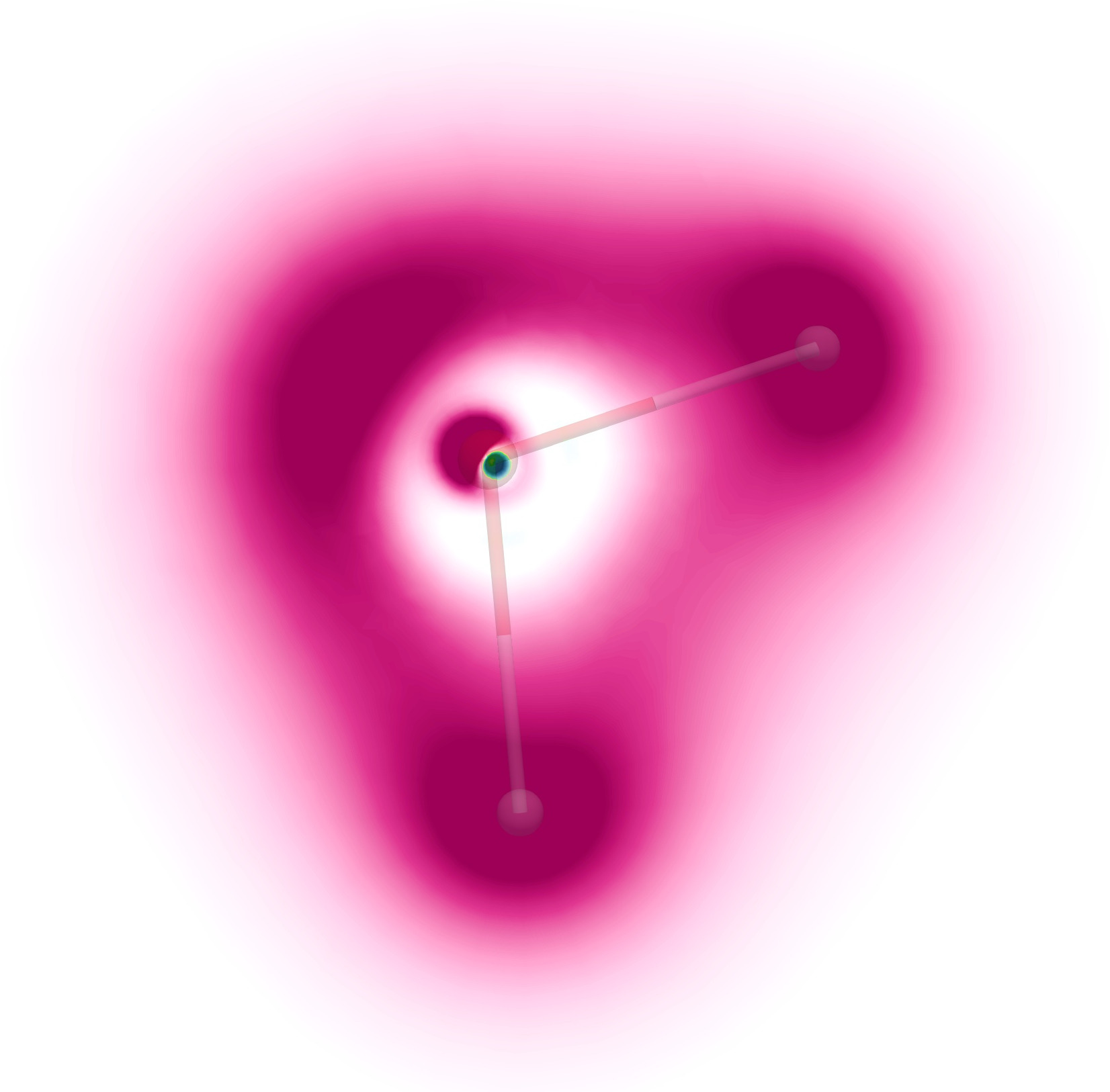
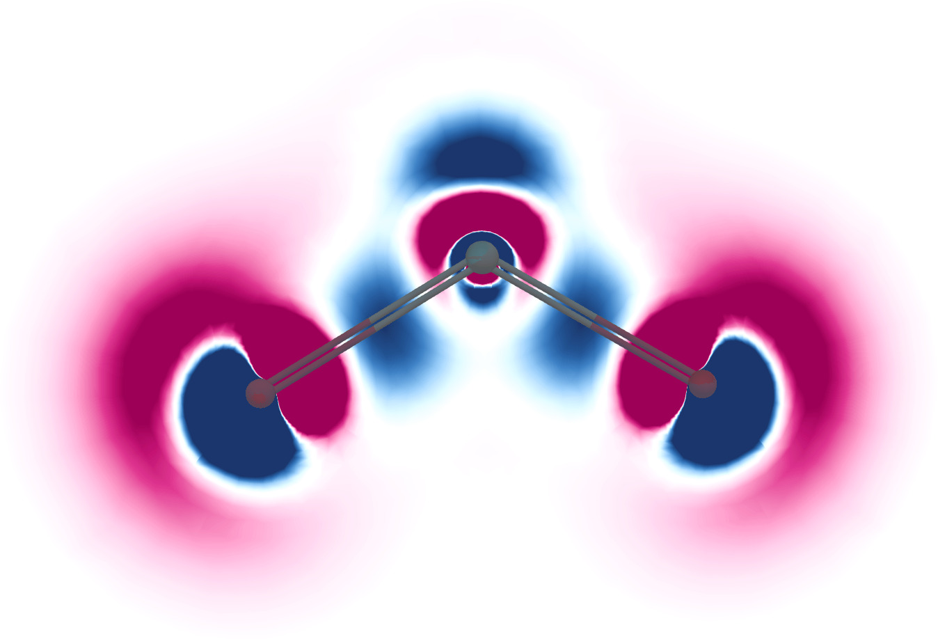
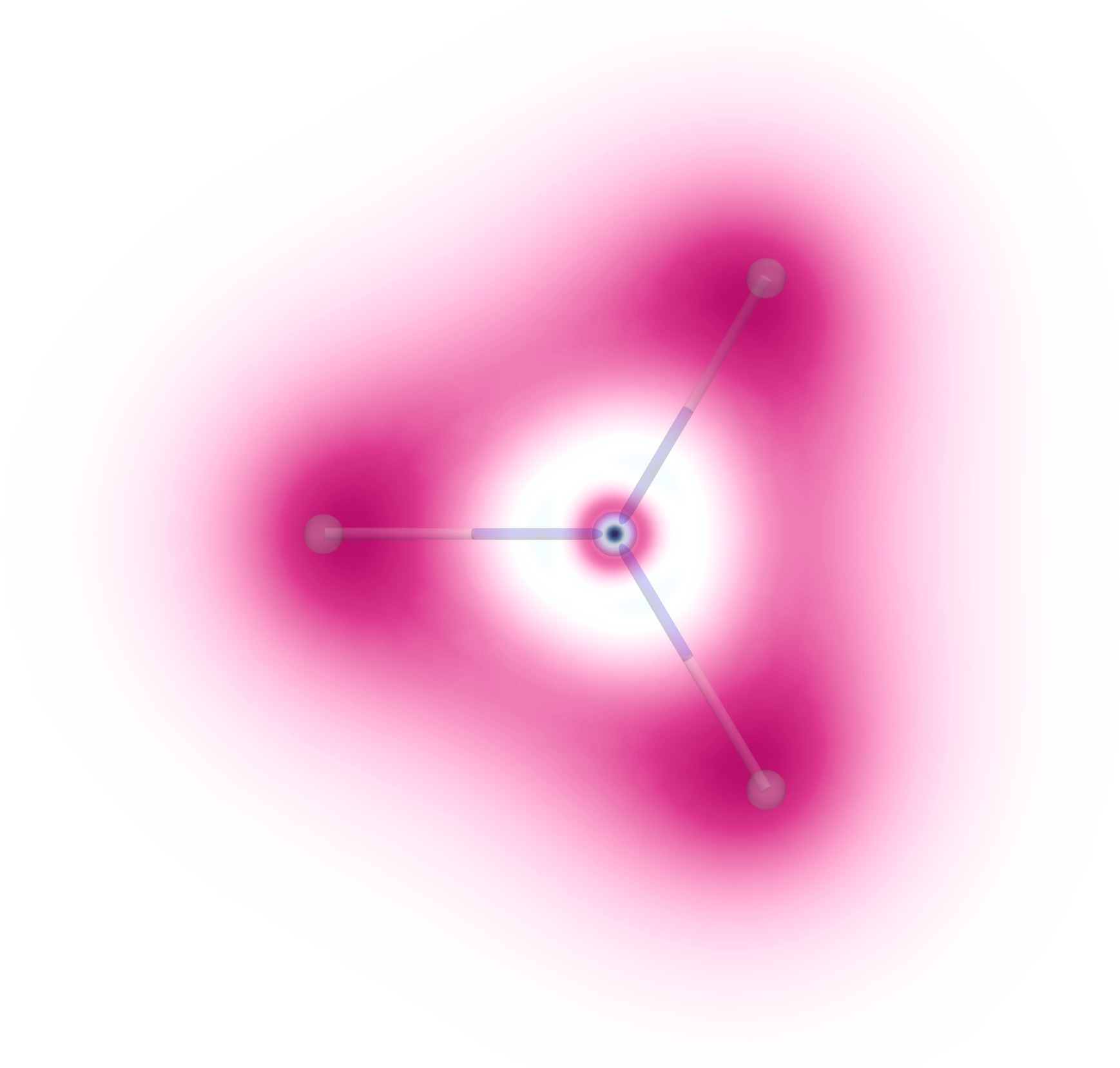
Figure 2: Visualization of the isotropic magnetizability density $\overline{\rho}^{\xi}({\bf r})$ ((LABEL:isomagdens)) shown in the molecular plane of H2O 2 and SO2 2 as well as in the plane formed by the hydrogen atoms of NH3 2, positioned $0.06\,a_{\mathrm{0}}$ away from the N atom towards the hydrogen atoms. Negative contributions are shown in pink, and positive ones in green. The gauge origin $\mathbf{R}_{O}$ is $(0,0,0)\mbox{$\,a_{\mathrm{0}}$}$

.

5.2 Magnetizability densities

Spatial contributions to the magnetizability densities, i.e., the integrand in (LABEL:Biot-Savart), are illustrated for H2O, NH3 and SO2 in magnetizability-function, with spaghetti showing the corresponding CDTs. The magnetizability densities are calculated with the gauge origin of the external magnetic field $(\mathbf{R}_{O})$ at $(x,y,z)=(0,0,0)$. In the calculations on H2O and SO2, the magnetic field perturbation is perpendicular to the molecular plane, while for NH3 the perturbation is parallel to the $C_{3}$ symmetry axis. In the case of H2O, the current-density flux around the whole molecule (spaghetti-h2o) leads to the ring-shaped contribution shown in magnetizability-function-h2o. The magnetic field along the symmetry axis of NH3 also results in a current-density flux around the molecule at the hydrogen atoms (spaghetti-nh3), giving rise to a similar ring-shaped contribution shown in magnetizability-function-nh3.

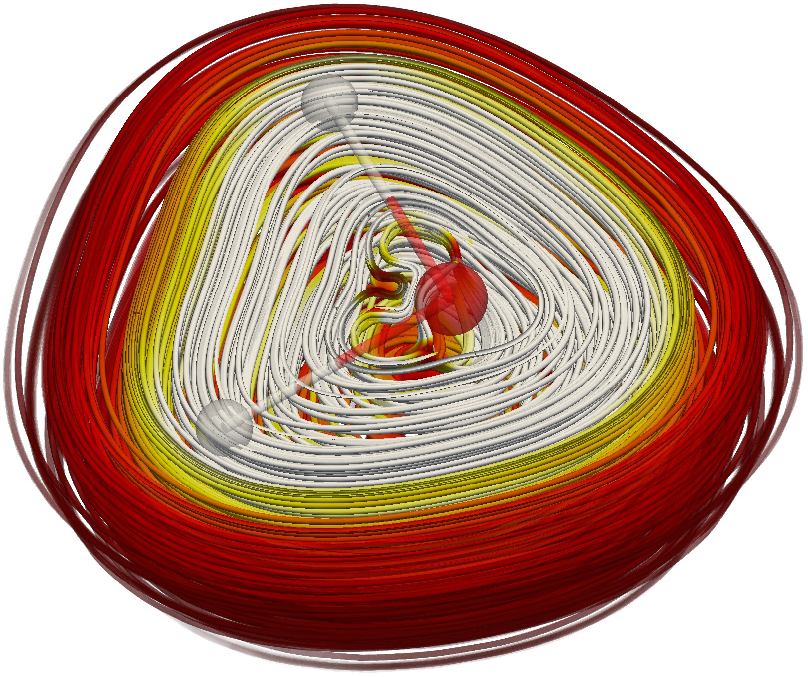
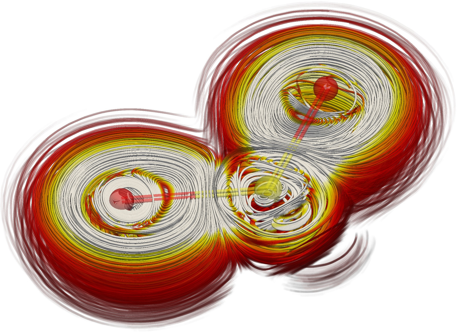
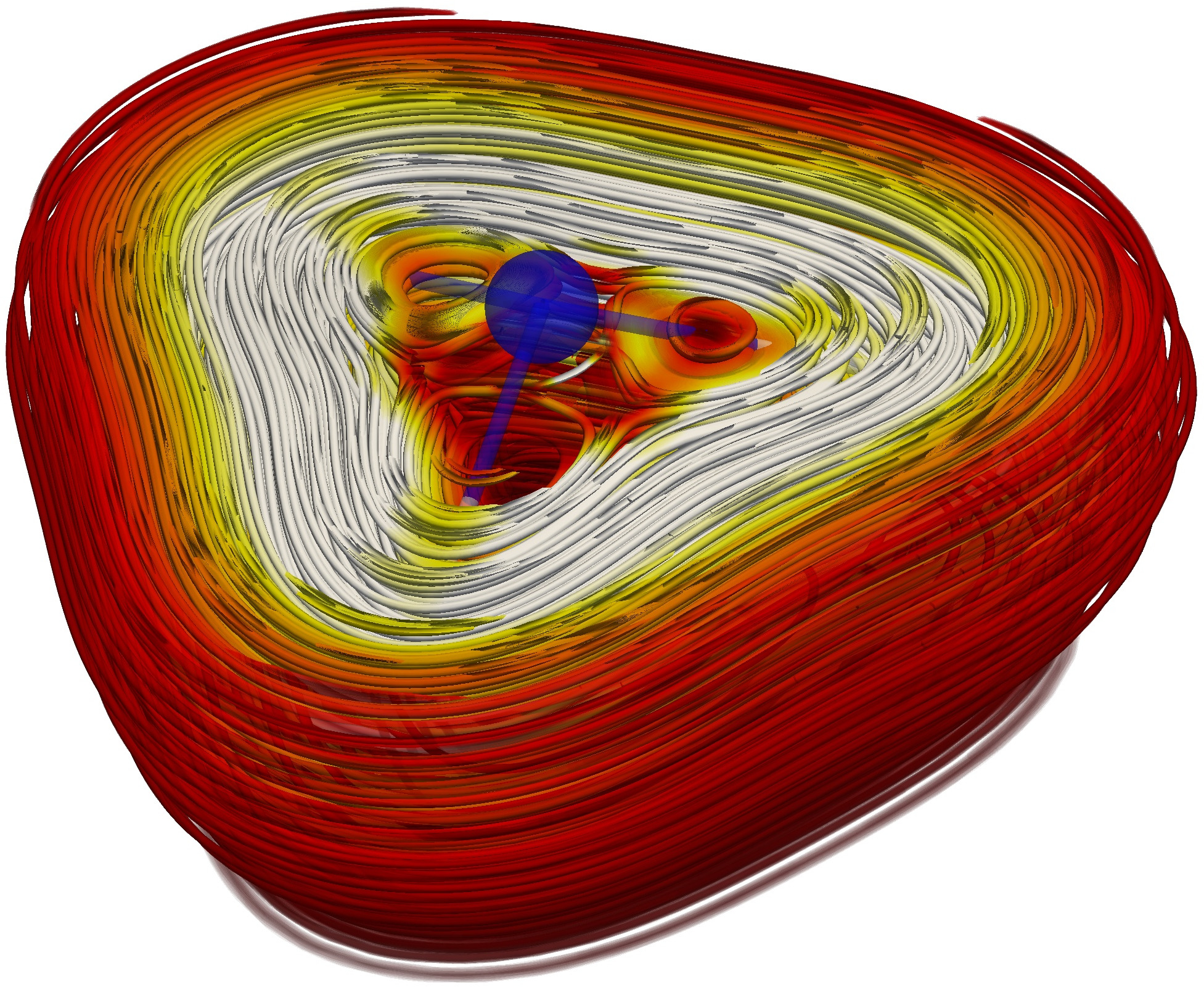
Figure 3: Streamline representation of the CDT ((LABEL:MCDSS)) of H2O (3), SO2 (3) and NH3 (3). The CDT is calculated with the magnetic field perpendicular to the molecular plane of H2O and SO2 as well as with it along the symmetry axis of NH3. The color scale represents the strength of the CDT in $\,{\rm nAT^{-1}}a_{0}^{-2}$.

The isotropic magnetizability density of SO2 shown in magnetizability-function-so2 has positive (green) and negative (pink) values. Calculations of the CDT show that the oxygens sustain a strong diatropic atomic CDT that flows around the atom, whereas the atomic CDT of the sulfur atom is much weaker (spaghetti-so2). The $p$-orbital shaped contributions to the magnetizability density of SO2 around the oxygens in magnetizability-function-so2 originate from the atomic CDTs. The patterns of the CDT of H2O and SO2 lead to the different magnetizability densities seen in magnetizability-function-h2o, magnetizability-function-so2, respectively. The positive magnetizability densities in H2O and NH3 are extremely localized close to the atomic nuclei, also because of vortices of the atomic CDT.

The magnetizability density depends on the gauge origin of the vector potential of the external magnetic field, even though the magnetizability is independent of the gauge origin.⁴³ The magnetizability densities for H2O, NH3 and SO2 calculated with the gauge origin at $\mathbf{R}_{O}=(1,1,1)\mbox{$\,a_{\mathrm{0}}$}$ are shown in the SI. The contribution of the choice of the gauge origin to the magnetizability computed from (LABEL:Biot-Savart) vanishes when the CDT fulfills the charge conservation condition²⁹

$$\int{\cal J}_{\alpha}^{B_{\beta}}(\mathbf{r})\mathrm{d}^{3}r=0.$$ (14)

Calculating the magnetizability for NH3 with a gauge origin set to $\mathbf{R}_{O}=(100,100,100)\mbox{$\,a_{\mathrm{0}}$}$ yielded a value that differs by 0.32% from the one computed for $\mathbf{R}_{O}=(0,0,0)$. When the gauge origin is set to $\mathbf{R}_{O}=(1,1,1)\mbox{$\,a_{\mathrm{0}}$}$, the deviation is two orders of magnitude smaller, because the change in the magnetizability depends linearly on the relative position of the gauge origin. The magnetizabilities of H2O and SO2 also change by only 0.46% and 0.03% when moving the gauge origin from $(0,0,0)\mbox{$\,a_{\mathrm{0}}$}$ to $(100,100,100)\mbox{$\,a_{\mathrm{0}}$}$, respectively, showing that that charge conservation is practically fulfilled in our calculations. All other positions than $(0,0,0)$ for the gauge origin lead to a spurious CDT contribution to the magnetizability density.

The GIAO ansatz modifies the atomic orbitals leading to a magnetic response of an external magnetic field that is correct to the first order for the one-center problem.^{30, 130} Even though they do not guarantee that the integral condition for the charge conservation of the CDT is fulfilled,¹³¹ the basis set convergence is faster and the leakage of the CDT is much smaller when GIAOs are used.³²

6 Conclusions

We have calculated magnetizabilities for a series of small molecules using both recently published density functionals, as well as older, established density functionals. The accuracy of the magnetizabilities predicted by the various density functional approximations has been assessed by comparison to coupled-cluster calculations with singles and doubles and perturbative triples [CCSD(T)] reported by Lutnæs et al. ¹⁸ Our results are summarized graphically in MAE-and-STD: the top functionals afford both small mean absolute errors and standard deviations, but the same is not true for all recently suggested functionals.

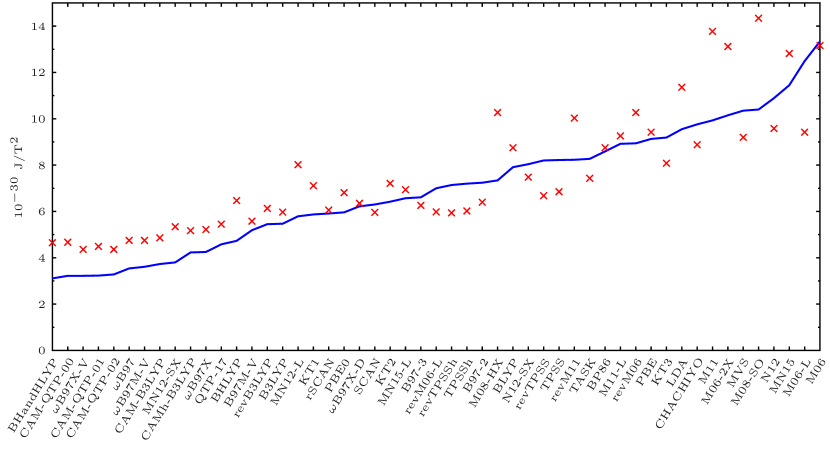
Figure 4: The mean absolute errors (blue solid line) as well as the errors’ standard deviations (red crosses) of the magnetizabilities in $10^{-30}\,{\rm J}/{\rm T}^{2}$) of the 27 studied molecules obtained with the 51 functionals compared to the CCSD(T) reference.

Numerical methods for calculating magnetizabilities based on quadrature of the magnetizability density have been implemented. We have shown that this method allows studies of spatial contributions to the magnetizabilities by visualization of the magnetizability density. The method has been employed to calculate magnetizabilities from magnetically induced current density susceptibilities, which were obtained from Turbomole calculations of nuclear magnetic shielding constants. Thus, magnetizabilities can be calculated in this way with Turbomole even though analytical methods to calculate magnetizabilities as the second derivative of the energy are not yet available in this program. Further information about spatial contributions to the magnetizability could be obtained in the present approach by studying atomic contributions and investigating the positive and negative parts of the integrands separately in analogy to our recent work on nuclear magnetic shieldings in ref. 53, which may be studied in future work.

Our calculations show that the most accurate magnetizabilities (judged by the smallest MAE) for the studied database are obtained with BHandHLYP, which is an old global hybrid with 50% HF exchange and 50% B88 exchange. The calculations also show that the modern range-separated functionals with 100% long-range HF exchange developed by Head-Gordon and co-workers and by Bartlett and co-workers yield accurate magnetizabilities for the database. Calculations with other range-separated functionals like CAM-B3LYP and CAMh-B3LYP as well as with global hybrid functionals like QTP-17, BHLYP a.k.a. BHandH, B3LYP and PBE0 yield relatively accurate magnetizabilities for the studied molecules. Meta-GGA functionals are found to yield somewhat better magnetizabilities than GGA and LDA functionals.

However, functionals developed by Truhlar and co-workers do not appear to be well-aimed for calculations of magnetizabilities and other magnetic properties that involve magnetically induced current densities. Magnetizabilities calculated using the popular M06-2X functional are found to be unreliable, and we do not recommend the use of the M06-2X functional in calculations of nuclear magnetic shieldings, magnetizabilities, ring-current strengths and other magnetic properties that depend on magnetically induced current density susceptibilities. Previous studies have also suggested that the M06-2X functional sometimes underestimates magnetizabilities and ring-current strengths.^{129, 128, 132} Revised versions of Minnesota functionals have been studied in this work, and found to yield somewhat more accurate magnetizabilities than the original parameterizations. However, the revised versions also still appear on the second half of the ranking list.

We thank Radovan Bast for help with the implementation of the numerical integration in Gimic using Numgrid. This work has been supported by the Academy of Finland (Suomen Akatemia) through project numbers 311149 and 314821, by the Magnus Ehrnrooth Foundation, and by The Swedish Cultural Foundation in Finland. We acknowledge computational resources from the Finnish Grid and Cloud Infrastructure (persistent identifier urn:nbn:fi:research-infras-2016072533) and CSC – IT Center for Science, Finland.

Contents:

• Magnetically induced current-density susceptibilitise

• Calculations on tetraoxa-isophlorin

• ST1: magnetizabilities for B3LYP, B97-2, B97-3, B97M-V, and BHandHLYP

• ST2: magnetizabilities for BHLYP, BLYP, BP86, and CAM-B3LYP

• ST3: magnetizabilities for CAMh-B3LYP, CAM-QTP-00, and CAM-QTP-01

• ST4: magnetizabilities for CAM-QTP-02, CHACHIYO, HF, KT1, KT2, and KT3

• ST5: magnetizabilities for LDA, M06, M06-2X, M06-L, M08-HX, and M08-SO

• ST6: magnetizabilities for M11, M11-L, MN12-L, MN12-SX, and MN15

• ST7: magnetizabilities for MN15-L, MVS, N12, N12-SX, PBE, and PBE0

• ST8: magnetizabilities for QTP-17, revB3LYP, revM06, and revM06-L

• ST9: magnetizabilities for revM11, revTPSS, revTPSSh, rSCAN, and SCAN

• ST10: magnetizabilities for TASK, TPSS, TPSSh, $\omega$B97, $\omega$B97M-V, and $\omega$B97X

• ST11: magnetizabilities for $\omega$B97X-D, and $\omega$B97X-V

• ST1d: magnetizability errors for B3LYP, B97-2, B97-3, B97M-V, and BHandHLYP

• ST2d: magnetizability errors for BHLYP, BLYP, BP86, and CAM-B3LYP

• ST3d: magnetizability errors for CAMh-B3LYP, CAM-QTP-00, and CAM-QTP-01

• ST4d: magnetizability errors for CAM-QTP-02, CHACHIYO, HF, KT1, KT2, and KT3

• ST5d: magnetizability errors for LDA, M06, M06-2X, M06-L, M08-HX, and M08-SO

• ST6d: magnetizability errors for M11, M11-L, MN12-L, MN12-SX, and MN15

• ST7d: magnetizability errors for MN15-L, MVS, N12, N12-SX, PBE, and PBE0

• ST8d: magnetizability errors for QTP-17, revB3LYP, revM06, and revM06-L

• ST9d: magnetizability errors for revM11, revTPSS, revTPSSh, rSCAN, and SCAN

• ST10d: magnetizability errors for TASK, TPSS, TPSSh, $\omega$B97, $\omega$B97M-V, and $\omega$B97X

• ST11d: magnetizability errors for $\omega$B97X-D, and $\omega$B97X-V

• comparison: comparison of Turbomole and PySCF data.

Magnetically induced current-density susceptibilities

$${\cal J}^{B_{\beta}}_{\alpha}=\frac{\partial J_{\alpha}^{\bf B}}{\partial B_{\beta}}\Bigg{|}_{{\bf B}={\bf 0}}=\sum_{\mu\nu}D_{\mu\nu}\left[\frac{\partial\chi^{*}_{\mu}(\mathbf{r})}{\partial B_{\beta}}\frac{\partial\tilde{h}\mathbf{(r)}}{\partial m_{I_{\alpha}}}\chi_{\nu}(\mathbf{r})+\chi^{*}_{\mu}(\mathbf{r})\frac{\partial\tilde{h}\mathbf{(r)}}{\partial m_{I\alpha}}\frac{\partial\chi_{\nu}(\mathbf{r})}{\partial B_{\beta}}\right.\\ \left.-\sum_{\gamma}\epsilon_{\alpha\beta\gamma}\chi^{*}_{\mu}(\mathbf{r})\frac{\partial^{2}\tilde{h}\mathbf{(r)}}{\partial m_{I_{\alpha}}\partial B_{\gamma}}\chi_{\nu}(\mathbf{r})\right]_{{\bf B}={\bf 0}}+\sum_{\mu\nu}\left[\frac{\partial D_{\mu\nu}}{\partial B_{\beta}}\chi^{*}_{\mu}(\mathbf{r})\frac{\partial\tilde{h}\mathbf{(r)}}{\partial m_{I_{\alpha}}}\chi_{\nu}(\mathbf{r})\right]_{{\bf B}={\bf 0}}.$$ (15)

Table 4: The expression used to calculate the magnetically induced current-density susceptibility (CDT).

The use of GIAOs eliminates the gauge origin ($\mathbf{R}_{O}$) from the expression we use for calculating the CDT, which is given in (LABEL:jexpression) in MCDS. In the expression, $\mathbf{p}$ is the momentum operator, $m_{I_{\alpha}}$ are the Cartesian components ($\alpha$) of the magnetic moment of nucleus $I$, $B_{\beta}$ are the Cartesian components ($\beta$) of the external magnetic field, $\mathbf{D}$ is the density matrix in the atomic-orbital basis, $[\partial\mathbf{D}/\partial\mathbf{B}]_{{\bf B}={\bf 0}}$ are the magnetically perturbed density matrices, $\epsilon_{\alpha\beta\gamma}$ is the Levi–Civita symbol, $\tilde{h}\mathbf{(r)}$ denotes the magnetic interaction operator without the $|\mathbf{r}-\mathbf{R}_{I}|^{-3}$ denominator with

$$\frac{\partial\tilde{h}\mathbf{(r)}}{\partial\mathbf{m}_{I}}=(\mathbf{r}-\mathbf{R}_{I})\times\mathbf{p}$$ (16)

and

$$\frac{\partial^{2}\tilde{h}\mathbf{(r)}}{\partial\mathbf{m}_{I}\partial\mathbf{B}}=\frac{1}{2}[(\mathbf{r}-\mathbf{R}_{O})\cdot(\mathbf{r}-\mathbf{R}_{I})\mathbf{1}-(\mathbf{r}-\mathbf{R}_{O})(\mathbf{r}-\mathbf{R}_{I})],$$ (17)

and $\mathbf{R}_{I}$ is the position of nucleus $I$. All terms that contain the gauge origin $\mathbf{R}_{O}$ cancel in (LABEL:jexpression), making the CDT calculation independent of the gauge origin; this is demonstrated in magnetizability-function2 for a different choice of the gauge origin. All terms containing the nuclear position $\mathbf{R}_{I}$ also cancel, eliminating explicit references to the nuclear coordinates.

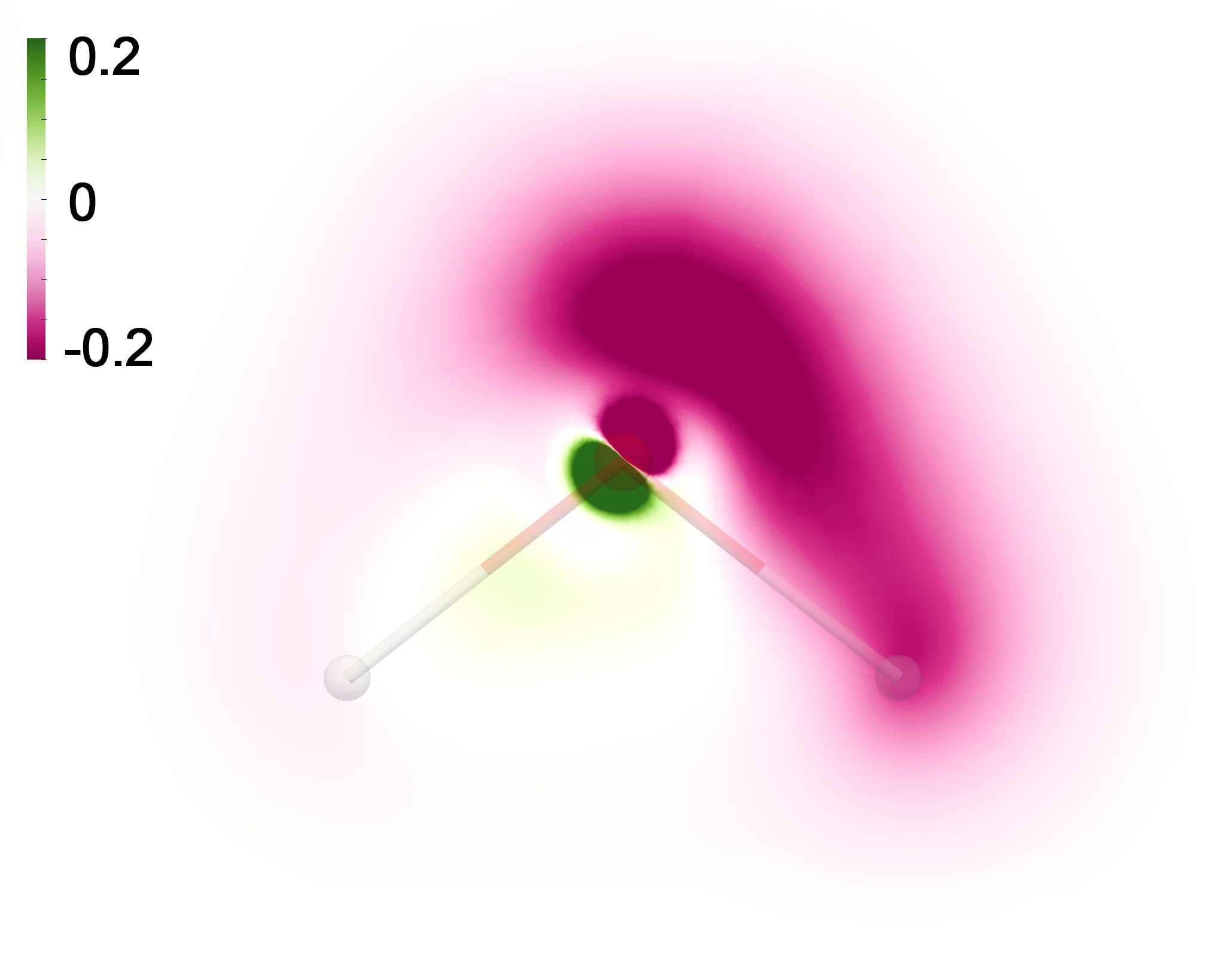
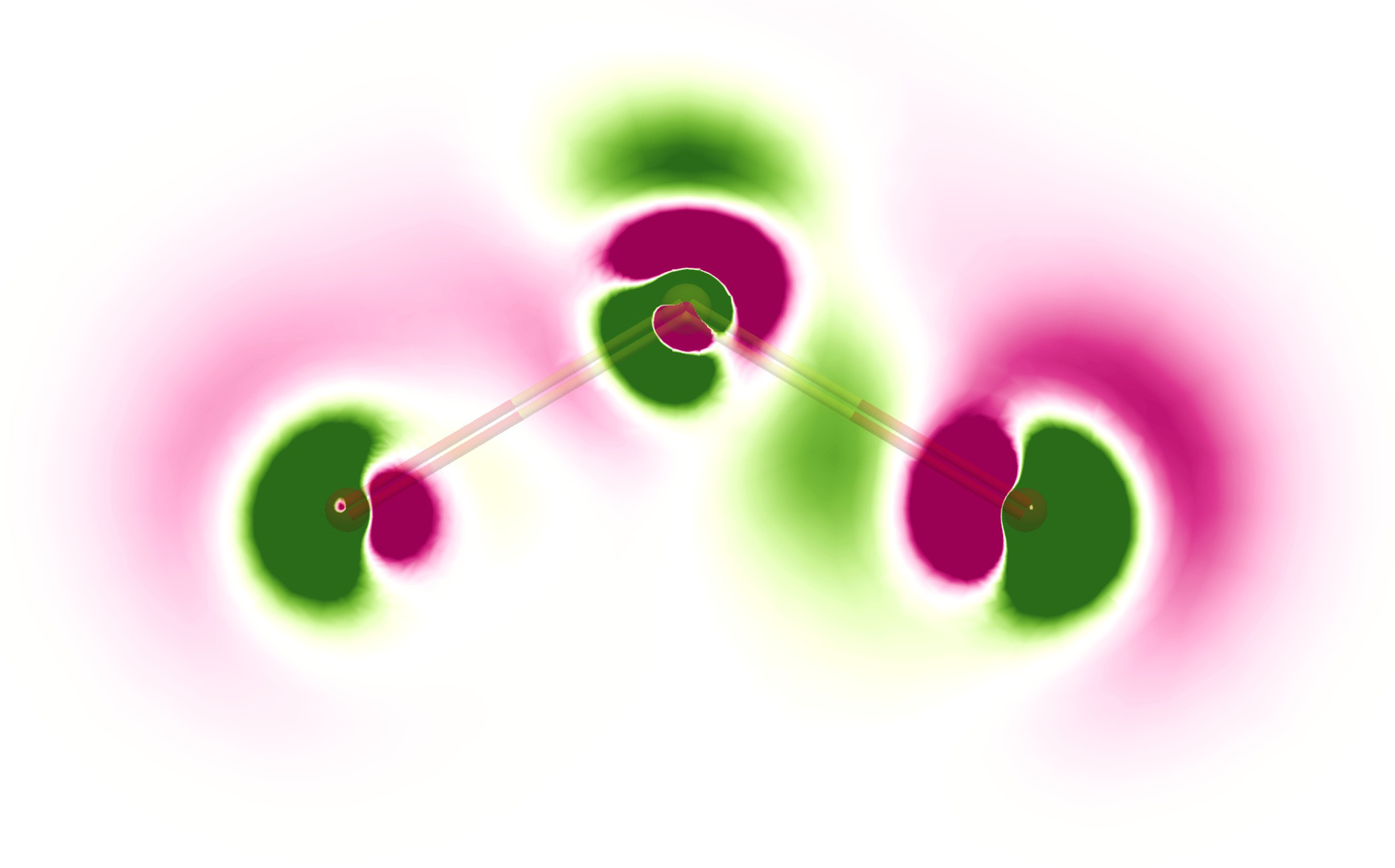
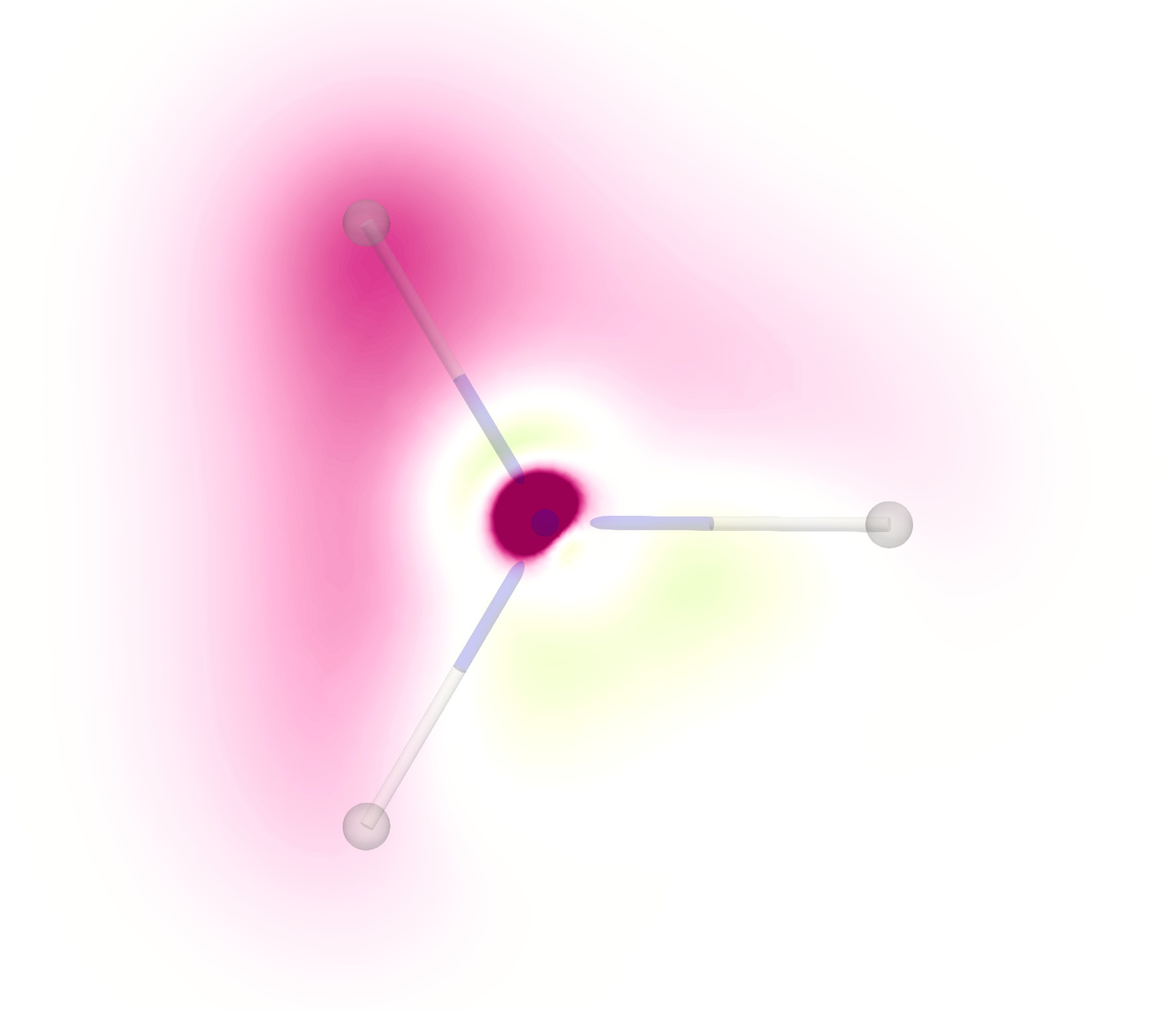
Figure 5: Visualization of the isotropic magnetizability density $\overline{\rho}^{\xi}({\bf r})$ shown in the molecular plane of H2O 5 and SO2 5 as well as in the plane formed by the hydrogen atoms of NH3 5, positioned $0.06\,a_{\mathrm{0}}$ away from the N atom towards the hydrogen atoms. Negative contributions are shown in pink, and positive ones in green. The gauge origin $\mathbf{R}_{O}$ is $(1,1,1)\mbox{$\,a_{\mathrm{0}}$}$.

Calculations on tetraoxa-isophlorin

Valiev et al. ¹²⁷ found the isotropic magnetizability of tetraoxa-isophlorin (molecule V in their work) to be 15.8 a.u. at the LMP2/cc-pVDZ level of theory [local second-order Møller–Plesset perturbation theory], while B3LYP/def2-TZVP calculations yielded a value of 65.9 a.u., which is over four times the LMP2 value. Repeating the calculations of Valiev et al. ¹²⁷ with the present approach using the def2-TZVP basis set, we obtained a magnetizability of 65.2 a.u. at the B3LYP level, which agrees within 1% with the value of Valiev et al. ¹²⁷; this difference can be tentatively attributed to the use of density fitting in the present work. MN12-SX, which has no exact exchange in the long range, predicts a susceptibility of 63.4 a.u., which is four times larger than the LMP2/cc-pVDZ value and close to the B3LYP value. Functionals with no exact exchange like PBE yield even larger values, $>100$ a.u. In contrast, calculations at the CAM-B3LYP level with 65% LR HF exchange yield a magnetizability of 20.7 a.u., which agrees well with the LMP2 reference value. BHandHLYP contains 50% LR HF exchange, and yields a magnetizability of 23.7 a.u., which is also in qualitative agreement with LMP2. Range-separated functionals with 100% LR HF exchange like $\omega$B97X and $\omega$B97 yield a magnetizability for tetraoxa-isophlorin that is close to zero or even negative like the HF value, which is $-11.6$ a.u.¹²⁷ The B3LYP/def2-TZVP optimized geometry of ref. 127, attached here in xyz format, was used in the calculations on tetraoxa-isophlorin.

Table 5: Magnetizabilities in units of $10^{-30}{\rm J}/{\rm T}^{2}$ for the B3LYP, B97-2, B97-3, B97M-V, and BHandHLYP functionals in the aug-cc-pCVQZ basis set from calculations with Turbomole and Gimic compared to CCSD(T) data from ref. 18.

Molecule	B3LYP	B97-2	B97-3	B97M-V	BHandHLYP	CCSD(T)
AlF	-396.5	-393.4	-392.6	-396.1	-395.6	-394.5
C2H4	-336.7	-334.3	-334.6	-334.8	-343.0	-345.6
C3H4	-463.1	-462.6	-464.1	-460.6	-468.8	-478.9
CH2O	-114.9	-116.6	-115.4	-132.8	-123.8	-127.4
CH3F	-312.4	-312.2	-313.3	-309.4	-314.9	-315.7
CH4	-317.0	-314.6	-314.6	-313.2	-315.7	-316.9
CO	-206.6	-202.5	-201.2	-208.5	-205.0	-209.5
FCCH	-440.1	-438.3	-439.2	-440.5	-443.6	-441.6
FCN	-367.4	-365.4	-365.9	-368.3	-370.5	-370.0
H2C2O	-422.1	-421.2	-421.0	-425.9	-425.0	-423.9
H2O	-236.7	-233.5	-233.9	-233.4	-234.0	-235.1
H2S	-455.1	-452.0	-452.4	-452.3	-453.5	-455.1
H4C2O	-526.9	-527.3	-529.0	-519.7	-534.5	-535.2
HCN	-269.4	-265.0	-265.4	-268.9	-272.7	-271.8
HCP	-487.4	-481.9	-482.9	-485.9	-494.3	-492.8
HF	-178.4	-175.9	-176.2	-176.1	-175.8	-176.4
HFCO	-300.5	-298.0	-298.0	-302.5	-304.0	-307.2
HOF	-231.1	-230.7	-232.2	-231.5	-236.7	-235.4
LiF	-194.7	-193.4	-194.5	-195.6	-192.6	-195.5
LiH	-130.8	-129.6	-127.0	-132.5	-126.4	-127.2
N2	-202.0	-197.2	-197.3	-203.2	-201.6	-205.2
N2O	-333.8	-332.6	-334.1	-333.0	-336.7	-339.1
NH3	-291.2	-287.9	-288.4	-287.0	-289.3	-290.3
O3	238.7	239.4	264.0	99.3	336.6	121.5
OCS	-579.6	-577.2	-578.8	-577.6	-585.6	-584.1
OF2	-234.1	-235.2	-238.2	-240.0	-250.2	-247.1
PN	-292.2	-285.4	-284.3	-302.0	-295.5	-308.2
SO2	-296.1	-289.5	-290.9	-301.3	-296.6	-314.3

Table 6: Magnetizabilities in units of $10^{-30}{\rm J}/{\rm T}^{2}$ for the BHLYP, BLYP, BP86, and CAM-B3LYP functionals in the aug-cc-pCVQZ basis set from calculations with Turbomole and Gimic compared to CCSD(T) data from ref. 18.

Molecule	BHLYP	BLYP	BP86	CAM-B3LYP	CCSD(T)
AlF	-397.1	-399.2	-394.3	-397.0	-394.5
C2H4	-343.5	-333.4	-331.0	-339.4	-345.6
C3H4	-473.1	-458.4	-460.1	-468.1	-478.9
CH2O	-114.1	-109.3	-108.1	-115.3	-127.4
CH3F	-319.0	-309.5	-311.4	-314.6	-315.7
CH4	-325.2	-318.1	-318.5	-320.0	-316.9
CO	-205.9	-209.1	-205.2	-208.4	-209.5
FCCH	-445.4	-438.5	-437.9	-441.8	-441.6
FCN	-371.6	-366.4	-365.0	-369.5	-370.0
H2C2O	-431.0	-420.7	-422.0	-424.8	-423.9
H2O	-236.6	-239.4	-237.5	-237.5	-235.1
H2S	-462.6	-457.0	-456.6	-456.7	-455.1
H4C2O	-542.1	-520.4	-523.5	-531.3	-535.2
HCN	-272.9	-268.7	-264.4	-272.0	-271.8
HCP	-492.9	-485.6	-479.2	-488.6	-492.8
HF	-177.0	-181.0	-179.3	-179.0	-176.4
HFCO	-303.8	-299.4	-296.5	-302.9	-307.2
HOF	-238.8	-226.7	-227.8	-233.4	-235.4
LiF	-193.1	-196.3	-197.0	-195.6	-195.5
LiH	-129.4	-136.5	-133.2	-129.3	-127.2
N2	-202.4	-203.7	-199.6	-204.3	-205.2
N2O	-338.8	-332.0	-332.6	-336.0	-339.1
NH3	-294.3	-293.4	-291.9	-292.7	-290.3
O3	356.9	180.1	180.9	258.1	121.5
OCS	-588.0	-576.1	-575.0	-583.4	-584.1
OF2	-251.5	-220.6	-222.1	-239.8	-247.1
PN	-293.9	-292.4	-284.7	-297.4	-308.2
SO2	-297.0	-298.4	-292.7	-300.7	-314.3

Table 7: Magnetizabilities in units of $10^{-30}{\rm J}/{\rm T}^{2}$ for the CAMh-B3LYP, CAM-QTP-00, and CAM-QTP-01 functionals in the aug-cc-pCVQZ basis set from calculations with Turbomole and Gimic compared to CCSD(T) data from ref. 18.

Molecule	CAMh-B3LYP	CAM-QTP-00	CAM-QTP-01	CCSD(T)
AlF	-396.9	-394.5	-397.2	-394.5
C2H4	-338.5	-344.7	-341.6	-345.6
C3H4	-466.2	-472.4	-471.9	-478.9
CH2O	-115.6	-124.5	-115.3	-127.4
CH3F	-313.6	-316.7	-316.6	-315.7
CH4	-318.6	-317.5	-322.7	-316.9
CO	-207.9	-205.2	-209.4	-209.5
FCCH	-441.2	-444.8	-443.5	-441.6
FCN	-368.8	-371.8	-371.2	-370.0
H2C2O	-423.6	-427.0	-427.4	-423.9
H2O	-237.2	-234.0	-238.0	-235.1
H2S	-455.8	-454.0	-458.5	-455.1
H4C2O	-529.5	-538.2	-535.6	-535.2
HCN	-271.2	-273.9	-273.9	-271.8
HCP	-488.4	-494.5	-489.8	-492.8
HF	-178.8	-175.5	-179.1	-176.4
HFCO	-302.2	-305.3	-304.5	-307.2
HOF	-232.5	-238.7	-235.6	-235.4
LiF	-195.4	-192.6	-195.8	-195.5
LiH	-129.8	-124.9	-128.6	-127.2
N2	-203.6	-202.3	-205.6	-205.2
N2O	-335.2	-338.2	-337.7	-339.1
NH3	-292.0	-289.8	-293.9	-290.3
O3	250.1	373.1	283.2	121.5
OCS	-582.1	-588.0	-586.4	-584.1
OF2	-237.7	-255.0	-244.9	-247.1
PN	-295.9	-297.6	-300.3	-308.2
SO2	-298.8	-298.6	-303.1	-314.3

Table 8: Magnetizabilities in units of $10^{-30}{\rm J}/{\rm T}^{2}$ for the CAM-QTP-02, CHACHIYO, HF, KT1, KT2, and KT3 functionals in the aug-cc-pCVQZ basis set from calculations with Turbomole and Gimic compared to CCSD(T) data from ref. 18.

Molecule	CAM-QTP-02	CHACHIYO	HF	KT1	KT2	KT3	CCSD(T)
AlF	-397.4	-392.2	-399.2	-398.4	-392.4	-394.2	-394.5
C2H4	-343.0	-329.0	-354.8	-338.6	-335.2	-332.4	-345.6
C3H4	-473.3	-458.7	-478.1	-461.5	-457.3	-453.2	-478.9
CH2O	-116.5	-109.3	-139.4	-116.8	-118.0	-117.9	-127.4
CH3F	-317.4	-310.8	-317.9	-309.8	-307.4	-305.3	-315.7
CH4	-323.3	-315.5	-313.6	-320.7	-316.0	-311.8	-316.9
CO	-209.3	-202.6	-204.5	-214.0	-209.1	-206.1	-209.5
FCCH	-444.5	-436.3	-452.2	-445.0	-440.2	-437.0	-441.6
FCN	-372.1	-363.4	-378.0	-372.4	-367.6	-365.1	-370.0
H2C2O	-428.6	-419.6	-432.6	-428.1	-422.1	-416.9	-423.9
H2O	-237.8	-235.9	-231.2	-238.8	-235.0	-233.8	-235.1
H2S	-459.1	-453.4	-452.6	-462.1	-455.7	-450.8	-455.1
H4C2O	-537.8	-522.2	-544.9	-527.0	-521.3	-516.5	-535.2
HCN	-274.8	-261.7	-280.1	-274.8	-270.5	-267.1	-271.8
HCP	-491.2	-475.5	-511.6	-493.6	-487.9	-483.9	-492.8
HF	-178.8	-178.4	-172.7	-179.8	-176.8	-176.5	-176.4
HFCO	-305.5	-294.7	-311.5	-303.3	-299.0	-297.5	-307.2
HOF	-237.1	-227.2	-244.6	-231.4	-227.6	-224.9	-235.4
LiF	-195.5	-196.1	-190.7	-199.1	-196.1	-193.8	-195.5
LiH	-128.0	-131.7	-125.3	-139.1	-137.1	-138.0	-127.2
N2	-205.9	-197.0	-202.9	-209.8	-205.0	-201.2	-205.2
N2O	-338.6	-331.6	-342.8	-334.6	-330.5	-328.0	-339.1
NH3	-294.1	-289.6	-287.4	-293.9	-289.6	-287.0	-290.3
O3	303.8	183.6	578.9	131.9	138.6	149.2	121.5
OCS	-587.9	-573.1	-597.5	-582.1	-575.6	-571.6	-584.1
OF2	-248.4	-222.1	-271.8	-231.7	-226.4	-223.3	-247.1
PN	-300.9	-279.9	-304.2	-302.1	-297.0	-291.1	-308.2
SO2	-303.7	-288.9	0.0	-304.6	-297.1	-292.6	-314.3

Table 9: Magnetizabilities in units of $10^{-30}{\rm J}/{\rm T}^{2}$ for the LDA, M06, M06-2X, M06-L, M08-HX, and M08-SO functionals in the aug-cc-pCVQZ basis set from calculations with Turbomole and Gimic compared to CCSD(T) data from ref. 18.

Molecule	LDA	M06	M06-2X	M06-L	M08-HX	M08-SO	CCSD(T)
AlF	-395.8	-387.1	-392.9	-382.7	-397.2	-395.8	-394.5
C2H4	-331.1	-332.4	-329.9	-327.1	-331.2	-334.3	-345.6
C3H4	-464.4	-465.3	-461.4	-461.5	-462.7	-463.7	-478.9
CH2O	-95.9	-104.5	-94.1	-123.6	-94.1	-89.4	-127.4
CH3F	-315.4	-313.4	-317.2	-311.1	-319.5	-319.0	-315.7
CH4	-329.4	-316.3	-319.9	-309.4	-322.6	-323.0	-316.9
CO	-206.6	-192.3	-193.9	-195.3	-201.7	-195.2	-209.5
FCCH	-438.6	-434.5	-439.7	-434.0	-442.4	-441.0	-441.6
FCN	-365.3	-358.7	-364.6	-359.9	-368.3	-365.2	-370.0
H2C2O	-427.7	-417.3	-418.1	-418.8	-423.1	-419.3	-423.9
H2O	-240.9	-233.1	-235.6	-230.2	-235.8	-236.7	-235.1
H2S	-466.0	-451.7	-457.7	-447.1	-457.1	-459.1	-455.1
H4C2O	-529.8	-529.4	-540.3	-521.1	-543.4	-543.5	-535.2
HCN	-265.1	-252.4	-260.4	-252.6	-265.2	-262.4	-271.8
HCP	-477.5	-465.0	-476.4	-462.9	-483.3	-480.5	-492.8
HF	-181.1	-175.1	-176.6	-173.8	-177.0	-177.5	-176.4
HFCO	-296.9	-292.1	-292.9	-292.4	-295.7	-293.5	-307.2
HOF	-229.0	-228.3	-235.1	-230.0	-236.4	-235.3	-235.4
LiF	-196.3	-190.4	-193.4	-191.8	-193.2	-193.0	-195.5
LiH	-136.0	-130.3	-128.1	-127.7	-129.1	-129.6	-127.2
N2	-201.1	-181.2	-189.1	-186.5	-195.7	-189.7	-205.2
N2O	-334.3	-326.3	-332.8	-329.0	-335.7	-331.7	-339.1
NH3	-298.1	-288.2	-291.9	-283.0	-292.0	-293.4	-290.3
O3	195.2	413.4	492.9	156.2	348.2	647.4	121.5
OCS	-576.6	-570.7	-578.3	-569.4	-583.5	-580.2	-584.1
OF2	-220.3	-228.5	-242.9	-234.3	-247.0	-241.6	-247.1
PN	-284.6	-249.4	-259.9	-267.0	-283.7	-259.9	-308.2
SO2	-295.1	-276.3	-277.4	-285.4	-287.7	-271.8	-314.3

Table 10: Magnetizabilities in units of $10^{-30}{\rm J}/{\rm T}^{2}$ for the M11, M11-L, MN12-L, MN12-SX, and MN15 functionals in the aug-cc-pCVQZ basis set from calculations with Turbomole and Gimic compared to CCSD(T) data from ref. 18.

Molecule	M11	M11-L	MN12-L	MN12-SX	MN15	CCSD(T)
AlF	-391.5	-403.1	-407.1	-403.4	-400.2	-394.5
C2H4	-331.3	-334.1	-340.4	-338.4	-330.4	-345.6
C3H4	-466.6	-461.3	-471.1	-467.1	-460.0	-478.9
CH2O	-89.0	-135.4	-145.0	-128.4	-91.0	-127.4
CH3F	-320.7	-307.8	-313.8	-315.5	-314.9	-315.7
CH4	-323.7	-312.0	-315.6	-317.7	-319.4	-316.9
CO	-199.2	-203.4	-211.4	-207.8	-194.3	-209.5
FCCH	-440.0	-444.9	-446.6	-445.2	-437.2	-441.6
FCN	-365.7	-368.1	-371.7	-370.9	-361.1	-370.0
H2C2O	-424.3	-431.4	-434.6	-428.8	-416.3	-423.9
H2O	-236.4	-227.8	-230.5	-233.4	-235.1	-235.1
H2S	-459.1	-450.6	-454.1	-454.8	-454.8	-455.1
H4C2O	-545.2	-518.5	-525.5	-532.5	-531.5	-535.2
HCN	-262.7	-263.9	-273.5	-271.6	-259.8	-271.8
HCP	-471.9	-489.0	-501.5	-494.9	-481.5	-492.8
HF	-177.9	-169.8	-173.5	-175.2	-176.8	-176.4
HFCO	-293.7	-300.3	-305.4	-303.3	-289.1	-307.2
HOF	-234.8	-228.6	-234.8	-237.4	-230.1	-235.4
LiF	-194.0	-188.3	-191.3	-190.8	-195.5	-195.5
LiH	-126.4	-150.0	-145.0	-140.5	-131.5	-127.2
N2	-193.7	-193.7	-204.3	-201.3	-186.9	-205.2
N2O	-334.5	-330.7	-336.1	-336.1	-328.4	-339.1
NH3	-292.7	-284.3	-286.3	-289.5	-291.0	-290.3
O3	484.4	84.9	45.6	131.1	571.0	121.5
OCS	-582.9	-579.9	-587.3	-586.0	-574.3	-584.1
OF2	-241.3	-242.3	-249.8	-253.4	-230.3	-247.1
PN	-266.2	-293.5	-330.2	-311.0	-271.6	-308.2
SO2	-273.4	-290.9	-312.3	-303.3	-268.9	-314.3

Table 11: Magnetizabilities in units of $10^{-30}{\rm J}/{\rm T}^{2}$ for the MN15-L, MVS, N12, N12-SX, PBE, and PBE0 functionals in the aug-cc-pCVQZ basis set from calculations with Turbomole and Gimic compared to CCSD(T) data from ref. 18.

Molecule	MN15-L	MVS	N12	N12-SX	PBE	PBE0	CCSD(T)
AlF	-410.2	-384.3	-394.1	-394.7	-396.9	-394.3	-394.5
C2H4	-343.2	-319.8	-331.1	-333.8	-330.8	-335.3	-345.6
C3H4	-470.4	-459.6	-456.3	-463.8	-459.5	-465.1	-478.9
CH2O	-142.4	-123.5	-112.9	-113.3	-104.9	-112.8	-127.4
CH3F	-314.1	-309.1	-307.8	-313.8	-311.2	-314.4	-315.7
CH4	-318.8	-315.1	-315.6	-316.5	-320.3	-318.4	-316.9
CO	-215.3	-198.0	-205.2	-201.1	-205.6	-202.9	-209.5
FCCH	-450.2	-436.9	-433.4	-436.2	-437.6	-439.9	-441.6
FCN	-376.7	-365.7	-360.8	-362.6	-365.0	-366.6	-370.0
H2C2O	-438.1	-428.8	-416.6	-419.6	-421.8	-423.6	-423.9
H2O	-235.8	-232.3	-234.3	-233.7	-238.5	-235.2	-235.1
H2S	-459.0	-456.0	-451.4	-453.9	-458.6	-456.2	-455.1
H4C2O	-530.1	-519.8	-516.6	-528.2	-523.9	-531.5	-535.2
HCN	-277.0	-256.3	-265.3	-264.0	-264.4	-266.0	-271.8
HCP	-508.5	-467.7	-477.2	-480.1	-479.3	-482.7	-492.8
HF	-176.9	-174.8	-176.2	-176.0	-180.1	-177.1	-176.4
HFCO	-309.6	-297.4	-294.8	-295.6	-296.8	-298.7	-307.2
HOF	-239.5	-226.7	-222.6	-230.0	-227.4	-232.8	-235.4
LiF	-197.3	-194.5	-191.7	-193.3	-196.2	-194.1	-195.5
LiH	-137.9	-125.5	-139.1	-128.9	-135.2	-129.1	-127.2
N2	-208.7	-191.9	-199.8	-195.5	-199.8	-198.2	-205.2
N2O	-340.0	-332.9	-326.5	-329.9	-331.8	-334.2	-339.1
NH3	-291.9	-287.4	-288.9	-288.6	-293.1	-290.4	-290.3
O3	63.6	136.6	185.3	292.9	183.4	257.6	121.5
OCS	-590.7	-576.0	-568.4	-576.7	-574.8	-579.6	-584.1
OF2	-255.0	-228.6	-217.6	-233.7	-221.6	-238.3	-247.1
PN	-330.5	-277.7	-285.9	-283.2	-284.3	-285.0	-308.2
SO2	-318.4	-289.8	-283.4	-284.2	-293.8	-291.5	-314.3

Table 12: Magnetizabilities in units of $10^{-30}{\rm J}/{\rm T}^{2}$ for the QTP-17, revB3LYP, revM06, and revM06-L functionals in the aug-cc-pCVQZ basis set from calculations with Turbomole and Gimic compared to CCSD(T) data from ref. 18.

Molecule	QTP-17	revB3LYP	revM06	revM06-L	CCSD(T)
AlF	-397.4	-396.9	-389.7	-385.9	-394.5
C2H4	-338.5	-337.0	-329.6	-326.6	-345.6
C3H4	-464.1	-463.6	-462.6	-461.2	-478.9
CH2O	-116.8	-113.8	-104.4	-134.0	-127.4
CH3F	-312.7	-312.8	-315.2	-310.5	-315.7
CH4	-316.9	-318.3	-318.4	-312.0	-316.9
CO	-207.1	-206.8	-197.2	-206.4	-209.5
FCCH	-441.1	-440.4	-438.2	-437.8	-441.6
FCN	-368.4	-367.7	-364.2	-366.5	-370.0
H2C2O	-422.8	-422.9	-421.1	-427.7	-423.9
H2O	-236.6	-237.1	-234.7	-230.8	-235.1
H2S	-455.3	-456.3	-456.3	-446.9	-455.1
H4C2O	-528.2	-527.8	-533.4	-517.3	-535.2
HCN	-270.8	-269.6	-261.3	-264.7	-271.8
HCP	-490.0	-487.5	-476.1	-478.4	-492.8
HF	-178.2	-178.6	-176.2	-174.4	-176.4
HFCO	-301.7	-300.7	-294.4	-298.9	-307.2
HOF	-232.2	-231.4	-232.7	-231.8	-235.4
LiF	-194.6	-194.8	-194.0	-195.1	-195.5
LiH	-130.9	-131.3	-127.8	-123.9	-127.2
N2	-202.7	-202.2	-191.7	-200.5	-205.2
N2O	-334.4	-334.1	-333.2	-334.6	-339.1
NH3	-291.2	-292.0	-290.6	-284.5	-290.3
O3	251.4	239.5	395.7	93.9	121.5
OCS	-581.2	-580.0	-578.1	-577.1	-584.1
OF2	-237.2	-234.2	-238.1	-241.0	-247.1
PN	-294.2	-292.3	-269.8	-305.2	-308.2
SO2	-297.1	-296.4	-280.9	-301.8	-314.3

Table 13: Magnetizabilities in units of $10^{-30}{\rm J}/{\rm T}^{2}$ for the revM11, revTPSS, revTPSSh, rSCAN, and SCAN functionals in the aug-cc-pCVQZ basis set from calculations with Turbomole and Gimic compared to CCSD(T) data from ref. 18.

Molecule	revM11	revTPSS	revTPSSh	rSCAN	SCAN	CCSD(T)
AlF	-393.5	-393.2	-392.7	-395.0	-392.0	-394.5
C2H4	-333.0	-332.0	-333.7	-332.3	-333.0	-345.6
C3H4	-467.4	-457.7	-460.2	-463.4	-462.4	-478.9
CH2O	-99.7	-123.2	-124.6	-121.9	-126.4	-127.4
CH3F	-316.8	-308.9	-310.3	-311.8	-310.4	-315.7
CH4	-320.1	-308.8	-309.3	-318.5	-314.4	-316.9
CO	-201.9	-204.9	-204.1	-206.7	-206.9	-209.5
FCCH	-437.8	-436.7	-437.8	-439.2	-438.3	-441.6
FCN	-365.4	-365.2	-365.9	-366.6	-365.8	-370.0
H2C2O	-418.7	-416.3	-417.7	-427.3	-426.0	-423.9
H2O	-238.1	-235.6	-234.6	-235.0	-234.2	-235.1
H2S	-456.2	-448.5	-448.7	-457.5	-453.9	-455.1
H4C2O	-538.2	-520.7	-523.9	-524.6	-519.8	-535.2
HCN	-264.1	-264.8	-265.5	-266.4	-265.3	-271.8
HCP	-473.1	-481.1	-482.5	-482.5	-481.7	-492.8
HF	-179.9	-178.5	-177.5	-176.8	-176.5	-176.4
HFCO	-298.1	-298.0	-298.9	-298.8	-299.3	-307.2
HOF	-233.8	-230.3	-232.2	-230.1	-230.9	-235.4
LiF	-196.9	-196.2	-195.3	-195.9	-195.6	-195.5
LiH	-123.4	-128.5	-127.2	-130.9	-130.4	-127.2
N2	-195.5	-199.0	-198.7	-201.4	-199.8	-205.2
N2O	-334.0	-331.3	-332.3	-333.6	-332.6	-339.1
NH3	-293.0	-287.5	-287.1	-290.3	-288.7	-290.3
O3	445.5	142.5	167.9	138.7	143.4	121.5
OCS	-580.8	-573.6	-575.8	-578.0	-577.7	-584.1
OF2	-239.0	-231.2	-236.8	-232.4	-234.3	-247.1
PN	-274.0	-288.1	-288.6	-294.8	-292.3	-308.2
SO2	-287.3	-291.7	-291.5	-297.5	-296.4	-314.3

Table 14: Magnetizabilities in units of $10^{-30}{\rm J}/{\rm T}^{2}$ for the TASK, TPSS, TPSSh, $\omega$B97, $\omega$B97M-V, and $\omega$B97X functionals in the aug-cc-pCVQZ basis set from calculations with Turbomole and Gimic compared to CCSD(T) data from ref. 18.

Molecule	TASK	TPSS	TPSSh	$\omega$B97	$\omega$B97M-V	$\omega$B97X	CCSD(T)
AlF	-383.3	-393.9	-393.3	-397.0	-400.1	-395.5	-394.5
C2H4	-325.4	-332.1	-333.8	-338.1	-340.5	-337.5	-345.6
C3H4	-460.8	-458.5	-460.9	-471.5	-469.9	-469.6	-478.9
CH2O	-132.9	-120.0	-121.7	-118.9	-115.8	-116.4	-127.4
CH3F	-309.3	-309.5	-310.9	-315.3	-315.0	-314.9	-315.7
CH4	-310.7	-311.6	-311.8	-318.7	-321.0	-317.9	-316.9
CO	-204.5	-204.7	-203.9	-208.2	-210.5	-205.8	-209.5
FCCH	-439.1	-436.7	-437.8	-442.1	-444.6	-441.2	-441.6
FCN	-367.8	-364.8	-365.5	-370.3	-371.8	-368.5	-370.0
H2C2O	-431.3	-417.9	-419.1	-427.0	-427.2	-424.6	-423.9
H2O	-231.2	-235.7	-234.7	-235.9	-237.3	-235.1	-235.1
H2S	-454.3	-450.6	-450.5	-454.2	-458.2	-454.3	-455.1
H4C2O	-519.1	-521.3	-524.5	-533.9	-533.9	-532.5	-535.2
HCN	-262.1	-264.4	-265.1	-269.5	-274.4	-268.6	-271.8
HCP	-478.2	-480.5	-481.9	-481.9	-491.0	-483.8	-492.8
HF	-173.7	-178.4	-177.3	-178.4	-178.7	-177.2	-176.4
HFCO	-298.6	-297.8	-298.6	-303.9	-304.0	-301.0	-307.2
HOF	-231.1	-229.3	-231.3	-234.5	-235.3	-233.5	-235.4
LiF	-195.1	-195.3	-194.6	-197.9	-196.3	-197.2	-195.5
LiH	-120.4	-129.5	-128.0	-126.4	-133.9	-129.3	-127.2
N2	-197.7	-198.8	-198.4	-202.4	-207.1	-200.6	-205.2
N2O	-335.7	-330.8	-331.8	-337.7	-337.5	-336.0	-339.1
NH3	-286.1	-288.4	-287.8	-290.3	-292.8	-289.9	-290.3
O3	142.9	151.0	176.9	236.9	225.4	260.5	121.5
OCS	-580.8	-573.6	-575.8	-585.6	-586.3	-583.2	-584.1
OF2	-236.8	-228.9	-234.8	-243.4	-245.4	-241.1	-247.1
PN	-289.1	-287.3	-287.7	-294.6	-300.7	-292.2	-308.2
SO2	-291.5	-291.9	-291.6	-300.8	-303.8	-296.5	-314.3

Table 15: Magnetizabilities in units of $10^{-30}{\rm J}/{\rm T}^{2}$ for the $\omega$B97X-D, and $\omega$B97X-V functionals in the aug-cc-pCVQZ basis set from calculations with Turbomole and Gimic compared to CCSD(T) data from ref. 18.

Molecule	$\omega$B97X-D	$\omega$B97X-V	CCSD(T)
AlF	-393.1	-396.5	-394.5
C2H4	-335.5	-338.9	-345.6
C3H4	-466.9	-469.9	-478.9
CH2O	-114.7	-118.6	-127.4
CH3F	-314.1	-314.9	-315.7
CH4	-316.1	-317.7	-316.9
CO	-202.4	-207.4	-209.5
FCCH	-439.8	-442.4	-441.6
FCN	-366.2	-370.1	-370.0
H2C2O	-422.1	-425.3	-423.9
H2O	-233.8	-236.0	-235.1
H2S	-452.9	-454.2	-455.1
H4C2O	-530.1	-532.8	-535.2
HCN	-266.2	-270.7	-271.8
HCP	-482.7	-486.5	-492.8
HF	-175.9	-178.1	-176.4
HFCO	-297.9	-303.1	-307.2
HOF	-232.0	-234.7	-235.4
LiF	-195.6	-196.4	-195.5
LiH	-131.5	-127.4	-127.2
N2	-197.7	-202.9	-205.2
N2O	-334.3	-336.8	-339.1
NH3	-288.7	-290.5	-290.3
O3	267.2	251.2	121.5
OCS	-579.6	-584.7	-584.1
OF2	-238.0	-243.8	-247.1
PN	-286.5	-296.0	-308.2
SO2	-290.6	-299.8	-314.3

Table 16: Deviations of the magnetizabilities computed with Turbomole and Gimic for the B3LYP, B97-2, B97-3, B97M-V, and BHandHLYP functionals in the aug-cc-pCVQZ basis set from CCSD(T) data from ref. 18 in units of $10^{-30}{\rm J}/{\rm T}^{2}$.

Molecule	B3LYP	B97-2	B97-3	B97M-V	BHandHLYP
AlF	-2.0	1.1	1.9	-1.6	-1.1
C2H4	8.9	11.3	11.0	10.8	2.6
C3H4	15.8	16.3	14.8	18.3	10.1
CH2O	12.5	10.8	12.0	-5.4	3.6
CH3F	3.3	3.5	2.4	6.3	0.8
CH4	-0.1	2.3	2.3	3.7	1.2
CO	2.9	7.0	8.3	1.0	4.5
FCCH	1.5	3.3	2.4	1.1	-2.0
FCN	2.6	4.6	4.1	1.7	-0.5
H2C2O	1.8	2.7	2.9	-2.0	-1.1
H2O	-1.6	1.6	1.2	1.7	1.1
H2S	-0.0	3.1	2.7	2.8	1.6
H4C2O	8.3	7.9	6.2	15.5	0.7
HCN	2.4	6.8	6.4	2.9	-0.9
HCP	5.4	10.9	9.9	6.9	-1.5
HF	-2.0	0.5	0.2	0.3	0.6
HFCO	6.7	9.2	9.2	4.7	3.2
HOF	4.3	4.7	3.2	3.9	-1.3
LiF	0.8	2.1	1.0	-0.1	2.9
LiH	-3.6	-2.4	0.2	-5.3	0.8
N2	3.2	8.0	7.9	2.0	3.6
N2O	5.3	6.5	5.0	6.1	2.4
NH3	-0.9	2.4	1.9	3.3	1.0
O3	117.2	117.9	142.5	-22.2	215.1
OCS	4.5	6.9	5.3	6.5	-1.5
OF2	13.0	11.9	8.9	7.1	-3.1
PN	16.0	22.8	23.9	6.2	12.7
SO2	18.2	24.8	23.4	13.0	17.7
MAE∗	5.5	7.2	6.6	5.2	3.1
ME∗	4.7	7.1	6.6	4.1	2.2
STD∗	6.0	6.4	6.3	5.6	4.7

• Statistics for the mean absolute error (MAE), mean error (ME) and the standard deviation (STD) exclude O3.

Table 17: Deviations of the magnetizabilities computed with Turbomole and Gimic for the BHLYP, BLYP, BP86, and CAM-B3LYP functionals in the aug-cc-pCVQZ basis set from CCSD(T) data from ref. 18 in units of $10^{-30}{\rm J}/{\rm T}^{2}$.

Molecule	BHLYP	BLYP	BP86	CAM-B3LYP
AlF	-2.6	-4.7	0.2	-2.5
C2H4	2.1	12.2	14.6	6.2
C3H4	5.8	20.5	18.8	10.8
CH2O	13.3	18.1	19.3	12.1
CH3F	-3.3	6.2	4.3	1.1
CH4	-8.3	-1.2	-1.6	-3.1
CO	3.6	0.4	4.3	1.1
FCCH	-3.8	3.1	3.7	-0.2
FCN	-1.6	3.6	5.0	0.5
H2C2O	-7.1	3.2	1.9	-0.9
H2O	-1.5	-4.3	-2.4	-2.4
H2S	-7.5	-1.9	-1.5	-1.6
H4C2O	-6.9	14.8	11.7	3.9
HCN	-1.1	3.1	7.4	-0.2
HCP	-0.1	7.2	13.6	4.2
HF	-0.6	-4.6	-2.9	-2.6
HFCO	3.4	7.8	10.7	4.3
HOF	-3.4	8.7	7.6	2.0
LiF	2.4	-0.8	-1.5	-0.1
LiH	-2.2	-9.3	-6.0	-2.1
N2	2.8	1.5	5.6	0.9
N2O	0.3	7.1	6.5	3.1
NH3	-4.0	-3.1	-1.6	-2.4
O3	235.4	58.6	59.4	136.6
OCS	-3.9	8.0	9.1	0.7
OF2	-4.4	26.5	25.0	7.3
PN	14.3	15.8	23.5	10.8
SO2	17.3	15.9	21.6	13.6
MAE∗	4.7	7.9	8.6	3.7
ME∗	0.1	5.7	7.3	2.4
STD∗	6.5	8.8	8.8	4.9

• Statistics for the mean absolute error (MAE), mean error (ME) and the standard deviation (STD) exclude O3.

Table 18: Deviations of the magnetizabilities computed with Turbomole and Gimic for the CAMh-B3LYP, CAM-QTP-00, and CAM-QTP-01 functionals in the aug-cc-pCVQZ basis set from CCSD(T) data from ref. 18 in units of $10^{-30}{\rm J}/{\rm T}^{2}$.

Molecule	CAMh-B3LYP	CAM-QTP-00	CAM-QTP-01
AlF	-2.4	-0.0	-2.7
C2H4	7.1	0.9	4.0
C3H4	12.7	6.5	7.0
CH2O	11.8	2.9	12.1
CH3F	2.1	-1.0	-0.9
CH4	-1.7	-0.6	-5.8
CO	1.6	4.3	0.1
FCCH	0.4	-3.2	-1.9
FCN	1.2	-1.8	-1.2
H2C2O	0.3	-3.1	-3.5
H2O	-2.1	1.1	-2.9
H2S	-0.7	1.1	-3.4
H4C2O	5.7	-3.0	-0.4
HCN	0.6	-2.1	-2.1
HCP	4.4	-1.7	3.0
HF	-2.4	0.9	-2.7
HFCO	5.0	1.9	2.7
HOF	2.9	-3.3	-0.2
LiF	0.1	2.9	-0.3
LiH	-2.6	2.3	-1.4
N2	1.6	2.9	-0.4
N2O	3.9	0.9	1.4
NH3	-1.7	0.5	-3.6
O3	128.6	251.6	161.7
OCS	2.0	-3.9	-2.3
OF2	9.4	-7.9	2.2
PN	12.3	10.6	7.9
SO2	15.5	15.7	11.2
MAE∗	4.2	3.2	3.2
ME∗	3.2	0.9	0.6
STD∗	5.2	4.7	4.5

• Statistics for the mean absolute error (MAE), mean error (ME) and the standard deviation (STD) exclude O3.

Table 19: Deviations of the magnetizabilities computed with Turbomole and Gimic for the CAM-QTP-02, CHACHIYO, HF, KT1, KT2, and KT3 functionals in the aug-cc-pCVQZ basis set from CCSD(T) data from ref. 18 in units of $10^{-30}{\rm J}/{\rm T}^{2}$.

Molecule	CAM-QTP-02	CHACHIYO	HF	KT1	KT2	KT3
AlF	-2.9	2.3	-4.7	-3.9	2.1	0.3
C2H4	2.6	16.6	-9.2	7.0	10.4	13.2
C3H4	5.6	20.2	0.8	17.4	21.6	25.7
CH2O	10.9	18.1	-12.0	10.6	9.4	9.5
CH3F	-1.7	4.9	-2.2	5.9	8.3	10.4
CH4	-6.4	1.4	3.3	-3.8	0.9	5.1
CO	0.2	6.9	5.0	-4.5	0.4	3.4
FCCH	-2.9	5.3	-10.6	-3.4	1.4	4.6
FCN	-2.1	6.6	-8.0	-2.4	2.4	4.9
H2C2O	-4.7	4.3	-8.7	-4.2	1.8	7.0
H2O	-2.7	-0.8	3.9	-3.7	0.1	1.3
H2S	-4.0	1.7	2.5	-7.0	-0.6	4.3
H4C2O	-2.6	13.0	-9.7	8.2	13.9	18.7
HCN	-3.0	10.1	-8.3	-3.0	1.3	4.7
HCP	1.6	17.3	-18.8	-0.8	4.9	8.9
HF	-2.4	-2.0	3.7	-3.4	-0.4	-0.1
HFCO	1.7	12.5	-4.3	3.9	8.2	9.7
HOF	-1.7	8.2	-9.2	4.0	7.8	10.5
LiF	0.0	-0.6	4.8	-3.6	-0.6	1.7
LiH	-0.8	-4.5	1.9	-11.9	-9.9	-10.8
N2	-0.7	8.2	2.3	-4.6	0.2	4.0
N2O	0.5	7.5	-3.7	4.5	8.6	11.1
NH3	-3.8	0.7	2.9	-3.6	0.7	3.3
O3	182.3	62.1	457.4	10.4	17.1	27.7
OCS	-3.8	11.0	-13.4	2.0	8.5	12.5
OF2	-1.3	25.0	-24.7	15.4	20.7	23.8
PN	7.3	28.3	4.0	6.1	11.2	17.1
SO2	10.6	25.4	314.3	9.7	17.2	21.7
MAE∗	3.3	9.8	18.4	5.9	6.4	9.2
ME∗	-0.2	9.2	7.5	1.1	5.6	8.4
STD∗	4.4	8.9	61.8	7.1	7.2	8.1

• Statistics for the mean absolute error (MAE), mean error (ME) and the standard deviation (STD) exclude O3.

Table 20: Deviations of the magnetizabilities computed with Turbomole and Gimic for the LDA, M06, M06-2X, M06-L, M08-HX, and M08-SO functionals in the aug-cc-pCVQZ basis set from CCSD(T) data from ref. 18 in units of $10^{-30}{\rm J}/{\rm T}^{2}$.

Molecule	LDA	M06	M06-2X	M06-L	M08-HX	M08-SO
AlF	-1.3	7.4	1.6	11.8	-2.7	-1.3
C2H4	14.5	13.2	15.7	18.5	14.4	11.3
C3H4	14.5	13.6	17.5	17.4	16.2	15.2
CH2O	31.5	22.9	33.3	3.8	33.3	38.0
CH3F	0.3	2.3	-1.5	4.6	-3.8	-3.3
CH4	-12.5	0.6	-3.0	7.5	-5.7	-6.1
CO	2.9	17.2	15.6	14.2	7.8	14.3
FCCH	3.0	7.1	1.9	7.6	-0.8	0.6
FCN	4.7	11.3	5.4	10.1	1.7	4.8
H2C2O	-3.8	6.6	5.8	5.1	0.8	4.6
H2O	-5.8	2.0	-0.5	4.9	-0.7	-1.6
H2S	-10.9	3.4	-2.6	8.0	-2.0	-4.0
H4C2O	5.4	5.8	-5.1	14.1	-8.2	-8.3
HCN	6.7	19.4	11.4	19.2	6.6	9.4
HCP	15.3	27.8	16.4	29.9	9.5	12.3
HF	-4.7	1.3	-0.2	2.6	-0.6	-1.1
HFCO	10.3	15.1	14.3	14.8	11.5	13.7
HOF	6.4	7.1	0.3	5.4	-1.0	0.1
LiF	-0.8	5.1	2.1	3.7	2.3	2.5
LiH	-8.8	-3.1	-0.9	-0.5	-1.9	-2.4
N2	4.1	24.0	16.1	18.7	9.5	15.5
N2O	4.8	12.8	6.3	10.1	3.4	7.4
NH3	-7.8	2.1	-1.6	7.3	-1.7	-3.1
O3	73.7	291.9	371.4	34.7	226.7	525.9
OCS	7.5	13.4	5.8	14.7	0.6	3.9
OF2	26.8	18.6	4.2	12.8	0.1	5.5
PN	23.6	58.8	48.3	41.2	24.5	48.3
SO2	19.2	38.0	36.9	28.9	26.6	42.5
MAE∗	9.6	13.3	10.1	12.5	7.3	10.4
ME∗	5.4	13.1	9.0	12.4	5.2	8.1
STD∗	11.4	13.2	13.1	9.4	10.3	14.3

• Statistics for the mean absolute error (MAE), mean error (ME) and the standard deviation (STD) exclude O3.

Table 21: Deviations of the magnetizabilities computed with Turbomole and Gimic for the M11, M11-L, MN12-L, MN12-SX, and MN15 functionals in the aug-cc-pCVQZ basis set from CCSD(T) data from ref. 18 in units of $10^{-30}{\rm J}/{\rm T}^{2}$.

Molecule	M11	M11-L	MN12-L	MN12-SX	MN15
AlF	3.0	-8.6	-12.6	-8.9	-5.7
C2H4	14.3	11.5	5.2	7.2	15.2
C3H4	12.3	17.6	7.8	11.8	18.9
CH2O	38.4	-8.0	-17.6	-1.0	36.4
CH3F	-5.0	7.9	1.9	0.2	0.8
CH4	-6.8	4.9	1.3	-0.8	-2.5
CO	10.3	6.1	-1.9	1.7	15.2
FCCH	1.6	-3.3	-5.0	-3.6	4.4
FCN	4.3	1.9	-1.7	-0.9	8.9
H2C2O	-0.4	-7.5	-10.7	-4.9	7.6
H2O	-1.3	7.3	4.6	1.7	-0.0
H2S	-4.0	4.5	1.0	0.3	0.3
H4C2O	-10.0	16.7	9.7	2.7	3.7
HCN	9.1	7.9	-1.7	0.2	12.0
HCP	20.9	3.8	-8.7	-2.1	11.3
HF	-1.5	6.6	2.9	1.2	-0.4
HFCO	13.5	6.9	1.8	3.9	18.1
HOF	0.6	6.8	0.6	-2.0	5.3
LiF	1.5	7.2	4.2	4.7	0.0
LiH	0.8	-22.8	-17.8	-13.3	-4.3
N2	11.5	11.5	0.9	3.9	18.3
N2O	4.6	8.4	3.0	3.0	10.7
NH3	-2.4	6.0	4.0	0.8	-0.7
O3	362.9	-36.6	-75.9	9.6	449.5
OCS	1.2	4.2	-3.2	-1.9	9.8
OF2	5.8	4.8	-2.7	-6.3	16.8
PN	42.0	14.7	-22.0	-2.8	36.6
SO2	40.9	23.4	2.0	11.0	45.4
MAE∗	9.9	8.9	5.8	3.8	11.4
ME∗	7.6	5.2	-2.0	0.2	10.4
STD∗	13.8	9.3	8.0	5.3	12.8

• Statistics for the mean absolute error (MAE), mean error (ME) and the standard deviation (STD) exclude O3.

Table 22: Deviations of the magnetizabilities computed with Turbomole and Gimic for the MN15-L, MVS, N12, N12-SX, PBE, and PBE0 functionals in the aug-cc-pCVQZ basis set from CCSD(T) data from ref. 18 in units of $10^{-30}{\rm J}/{\rm T}^{2}$.

Molecule	MN15-L	MVS	N12	N12-SX	PBE	PBE0
AlF	-15.7	10.2	0.4	-0.2	-2.4	0.2
C2H4	2.4	25.8	14.5	11.8	14.8	10.3
C3H4	8.5	19.3	22.6	15.1	19.4	13.8
CH2O	-15.0	3.9	14.5	14.1	22.5	14.6
CH3F	1.6	6.6	7.9	1.9	4.5	1.3
CH4	-1.9	1.8	1.3	0.4	-3.4	-1.5
CO	-5.8	11.5	4.3	8.4	3.9	6.6
FCCH	-8.6	4.7	8.2	5.4	4.0	1.7
FCN	-6.7	4.3	9.2	7.4	5.0	3.4
H2C2O	-14.2	-4.9	7.3	4.3	2.1	0.3
H2O	-0.7	2.8	0.8	1.4	-3.4	-0.1
H2S	-3.9	-0.9	3.7	1.2	-3.5	-1.1
H4C2O	5.1	15.4	18.6	7.0	11.3	3.7
HCN	-5.2	15.5	6.5	7.8	7.4	5.8
HCP	-15.7	25.1	15.6	12.7	13.5	10.1
HF	-0.5	1.6	0.2	0.4	-3.7	-0.7
HFCO	-2.4	9.8	12.4	11.6	10.4	8.5
HOF	-4.1	8.7	12.8	5.4	8.0	2.6
LiF	-1.8	1.0	3.8	2.2	-0.7	1.4
LiH	-10.7	1.7	-11.9	-1.7	-8.0	-1.9
N2	-3.5	13.3	5.4	9.7	5.4	7.0
N2O	-0.9	6.2	12.6	9.2	7.3	4.9
NH3	-1.6	2.9	1.4	1.7	-2.8	-0.1
O3	-57.9	15.1	63.8	171.4	61.9	136.1
OCS	-6.6	8.1	15.7	7.4	9.3	4.5
OF2	-7.9	18.5	29.5	13.4	25.5	8.8
PN	-22.3	30.5	22.3	25.0	23.9	23.2
SO2	-4.1	24.5	30.9	30.1	20.5	22.8
MAE∗	6.6	10.4	10.9	8.0	9.1	6.0
ME∗	-5.3	9.9	10.0	7.9	7.1	5.6
STD∗	6.9	9.2	9.6	7.5	9.4	6.8

• Statistics for the mean absolute error (MAE), mean error (ME) and the standard deviation (STD) exclude O3.

Table 23: Deviations of the magnetizabilities computed with Turbomole and Gimic for the QTP-17, revB3LYP, revM06, and revM06-L functionals in the aug-cc-pCVQZ basis set from CCSD(T) data from ref. 18 in units of $10^{-30}{\rm J}/{\rm T}^{2}$.

Molecule	QTP-17	revB3LYP	revM06	revM06-L
AlF	-2.9	-2.4	4.8	8.6
C2H4	7.1	8.6	16.0	19.0
C3H4	14.8	15.3	16.3	17.7
CH2O	10.6	13.6	23.0	-6.6
CH3F	3.0	2.9	0.5	5.2
CH4	-0.0	-1.4	-1.5	4.9
CO	2.4	2.7	12.3	3.1
FCCH	0.5	1.2	3.4	3.8
FCN	1.6	2.3	5.8	3.5
H2C2O	1.1	1.0	2.8	-3.8
H2O	-1.5	-2.0	0.4	4.3
H2S	-0.2	-1.2	-1.2	8.2
H4C2O	7.0	7.4	1.8	17.9
HCN	1.0	2.2	10.5	7.1
HCP	2.8	5.3	16.7	14.4
HF	-1.8	-2.2	0.2	2.0
HFCO	5.5	6.5	12.8	8.3
HOF	3.2	4.0	2.7	3.6
LiF	0.9	0.7	1.5	0.4
LiH	-3.7	-4.1	-0.6	3.3
N2	2.5	3.0	13.5	4.7
N2O	4.7	5.0	5.9	4.5
NH3	-0.9	-1.7	-0.3	5.8
O3	129.9	118.0	274.2	-27.6
OCS	2.9	4.1	6.0	7.0
OF2	9.9	12.9	9.0	6.1
PN	14.0	15.9	38.4	3.0
SO2	17.2	17.9	33.4	12.5
MAE∗	4.6	5.4	8.9	7.0
ME∗	3.8	4.3	8.7	6.2
STD∗	5.4	6.1	10.3	6.0

• Statistics for the mean absolute error (MAE), mean error (ME) and the standard deviation (STD) exclude O3.

Table 24: Deviations of the magnetizabilities computed with Turbomole and Gimic for the revM11, revTPSS, revTPSSh, rSCAN, and SCAN functionals in the aug-cc-pCVQZ basis set from CCSD(T) data from ref. 18 in units of $10^{-30}{\rm J}/{\rm T}^{2}$.

Molecule	revM11	revTPSS	revTPSSh	rSCAN	SCAN
AlF	1.0	1.3	1.8	-0.5	2.5
C2H4	12.6	13.6	11.9	13.3	12.6
C3H4	11.5	21.2	18.7	15.5	16.5
CH2O	27.7	4.2	2.8	5.5	1.0
CH3F	-1.1	6.8	5.4	3.9	5.3
CH4	-3.2	8.1	7.6	-1.6	2.5
CO	7.6	4.6	5.4	2.8	2.6
FCCH	3.8	4.9	3.8	2.4	3.3
FCN	4.6	4.8	4.1	3.4	4.2
H2C2O	5.2	7.6	6.2	-3.4	-2.1
H2O	-3.0	-0.5	0.5	0.1	0.9
H2S	-1.1	6.6	6.4	-2.4	1.2
H4C2O	-3.0	14.5	11.3	10.6	15.4
HCN	7.7	7.0	6.3	5.4	6.5
HCP	19.7	11.7	10.3	10.3	11.1
HF	-3.5	-2.1	-1.1	-0.4	-0.1
HFCO	9.1	9.2	8.3	8.4	7.9
HOF	1.6	5.1	3.2	5.3	4.5
LiF	-1.4	-0.7	0.2	-0.4	-0.1
LiH	3.8	-1.3	-0.0	-3.7	-3.2
N2	9.7	6.2	6.5	3.8	5.4
N2O	5.1	7.8	6.8	5.5	6.5
NH3	-2.7	2.8	3.2	-0.0	1.6
O3	324.0	21.0	46.4	17.2	21.9
OCS	3.3	10.5	8.3	6.1	6.4
OF2	8.1	15.9	10.3	14.7	12.8
PN	34.2	20.1	19.6	13.4	15.9
SO2	27.0	22.6	22.8	16.8	17.9
MAE∗	8.2	8.2	7.1	5.9	6.3
ME∗	6.8	7.9	7.1	5.0	5.9
STD∗	10.0	6.7	5.9	6.1	6.0

• Statistics for the mean absolute error (MAE), mean error (ME) and the standard deviation (STD) exclude O3.

Table 25: Deviations of the magnetizabilities computed with Turbomole and Gimic for the TASK, TPSS, TPSSh, $\omega$B97, $\omega$B97M-V, and $\omega$B97X functionals in the aug-cc-pCVQZ basis set from CCSD(T) data from ref. 18 in units of $10^{-30}{\rm J}/{\rm T}^{2}$.

Molecule	TASK	TPSS	TPSSh	$\omega$B97	$\omega$B97M-V	$\omega$B97X
AlF	11.2	0.6	1.2	-2.5	-5.6	-1.0
C2H4	20.2	13.5	11.8	7.5	5.1	8.1
C3H4	18.1	20.4	18.0	7.4	9.0	9.3
CH2O	-5.5	7.4	5.7	8.5	11.6	11.0
CH3F	6.4	6.2	4.8	0.4	0.7	0.8
CH4	6.2	5.3	5.1	-1.8	-4.1	-1.0
CO	5.0	4.8	5.6	1.3	-1.0	3.7
FCCH	2.5	4.9	3.8	-0.5	-3.0	0.4
FCN	2.2	5.2	4.5	-0.3	-1.8	1.5
H2C2O	-7.4	6.0	4.8	-3.1	-3.3	-0.7
H2O	3.9	-0.6	0.4	-0.8	-2.2	-0.0
H2S	0.8	4.5	4.6	0.9	-3.1	0.8
H4C2O	16.1	13.9	10.7	1.3	1.3	2.7
HCN	9.7	7.4	6.7	2.3	-2.6	3.2
HCP	14.6	12.3	10.9	10.9	1.8	9.0
HF	2.7	-2.0	-0.9	-2.0	-2.3	-0.8
HFCO	8.6	9.4	8.6	3.3	3.2	6.2
HOF	4.3	6.1	4.1	0.9	0.1	1.9
LiF	0.4	0.2	0.9	-2.4	-0.8	-1.7
LiH	6.8	-2.3	-0.8	0.8	-6.7	-2.1
N2	7.5	6.4	6.8	2.8	-1.9	4.6
N2O	3.4	8.3	7.3	1.4	1.6	3.1
NH3	4.2	1.9	2.5	0.0	-2.5	0.4
O3	21.4	29.5	55.4	115.4	103.9	139.0
OCS	3.3	10.5	8.3	-1.5	-2.2	0.9
OF2	10.3	18.2	12.3	3.7	1.7	6.0
PN	19.1	20.9	20.5	13.6	7.5	16.0
SO2	22.8	22.4	22.7	13.5	10.5	17.8
MAE∗	8.3	8.2	7.2	3.5	3.6	4.2
ME∗	7.3	7.8	7.1	2.4	0.4	3.7
STD∗	7.4	6.8	6.0	4.8	4.8	5.2

• Statistics for the mean absolute error (MAE), mean error (ME) and the standard deviation (STD) exclude O3.

Table 26: Deviations of the magnetizabilities computed with Turbomole and Gimic for the $\omega$B97X-D, and $\omega$B97X-V functionals in the aug-cc-pCVQZ basis set from CCSD(T) data from ref. 18 in units of $10^{-30}{\rm J}/{\rm T}^{2}$.

Molecule	$\omega$B97X-D	$\omega$B97X-V
AlF	1.4	-2.0
C2H4	10.1	6.7
C3H4	12.0	9.0
CH2O	12.7	8.8
CH3F	1.6	0.8
CH4	0.8	-0.8
CO	7.1	2.1
FCCH	1.8	-0.8
FCN	3.8	-0.1
H2C2O	1.8	-1.4
H2O	1.3	-0.9
H2S	2.2	0.9
H4C2O	5.1	2.4
HCN	5.6	1.1
HCP	10.1	6.3
HF	0.5	-1.7
HFCO	9.3	4.1
HOF	3.4	0.7
LiF	-0.1	-0.9
LiH	-4.3	-0.2
N2	7.5	2.3
N2O	4.8	2.3
NH3	1.6	-0.2
O3	145.7	129.7
OCS	4.5	-0.6
OF2	9.1	3.3
PN	21.7	12.2
SO2	23.7	14.5
MAE∗	6.2	3.2
ME∗	5.9	2.5
STD∗	6.3	4.4

• Statistics for the mean absolute error (MAE), mean error (ME) and the standard deviation (STD) exclude O3.

Table 27: Comparison of the magnetizabilities in $10^{-30}{\rm J}/{\rm T}^{2}$ calculated with Turbomole (TM) /Gimic employing the resolution of the identity approximation, and PySCF employing exact integrals at the BP86/aug-cc-pCVQZ and B3LYP/aug-cc-pCVQZ levels of theory. The PySCF data is in full agreement with that from Gaussian.

Molecule	BP86			B3LYP
	Tm/Gimic	PySCF	difference	Tm/Gimic	PySCF	difference
AlF	-394.3	-394.4	0.2	-396.5	-396.6	0.1
C2H4	-331.0	-330.9	-0.0	-336.7	-336.7	-0.0
C3H4	-460.1	-460.1	-0.0	-463.1	-463.0	-0.0
CH2O	-108.1	-108.1	0.0	-114.9	-114.9	0.0
CH3F	-311.4	-311.4	0.0	-312.4	-312.4	0.0
CH4	-318.5	-318.6	0.1	-317.0	-317.1	0.1
CO	-205.2	-205.2	0.0	-206.6	-206.6	0.0
FCCH	-437.9	-437.9	-0.0	-440.1	-440.0	-0.0
FCN	-365.0	-365.0	0.0	-367.4	-367.4	-0.0
H2C2O	-422.0	-422.1	0.1	-422.1	-422.2	0.1
H2O	-237.5	-237.5	0.1	-236.7	-236.7	0.0
H2S	-456.6	-456.7	0.2	-455.1	-455.3	0.2
H4C2O	-523.5	-523.5	0.0	-526.9	-526.9	-0.0
HCN	-264.4	-264.4	0.0	-269.4	-269.4	0.0
HCP	-479.2	-479.3	0.0	-487.4	-487.4	-0.0
HF	-179.3	-179.3	0.0	-178.4	-178.4	0.0
HFCO	-296.5	-296.5	0.0	-300.5	-300.5	0.0
HOF	-227.8	-227.7	-0.0	-231.1	-231.1	-0.0
LiF	-197.0	-197.1	0.1	-194.7	-194.8	0.1
LiH	-133.2	-133.2	-0.0	-130.8	-130.7	-0.0
N2	-199.6	-199.5	-0.1	-202.0	-201.9	-0.1
N2O	-332.6	-332.7	0.1	-333.8	-334.0	0.1
NH3	-291.9	-292.0	0.1	-291.2	-291.3	0.1
O3	180.9	181.2	-0.3	238.7	239.0	-0.3
OCS	-575.0	-575.1	0.1	-579.6	-579.7	0.1
OF2	-222.1	-221.8	-0.2	-234.1	-233.9	-0.2
PN	-284.7	-284.3	-0.4	-292.2	-291.8	-0.4
SO2	-292.7	-292.3	-0.5	-296.1	-295.6	-0.4

References

- Becke 1988 Becke, A. D. Density-functional exchange-energy approximation with correct asymptotic behavior. Phys. Rev. A 1988, 38, 3098
- Perdew 1986 Perdew, J. P. Density-functional approximation for the correlation energy of the inhomogeneous electron gas. Phys. Rev. B 1986, 33, 8822
- Lee et al. 1988 Lee, C.; Yang, W.; Parr, R. G. Development of the Colle–Salvetti correlation-energy formula into a functional of the electron density. Phys. Rev. B 1988, 37, 785
- Perdew et al. 1996 Perdew, J. P.; Burke, K.; Ernzerhof, M. Generalized Gradient Approximation Made Simple. Phys. Rev. Lett. 1996, 77, 3865
- Perdew et al. 1997 Perdew, J. P.; Burke, K.; Ernzerhof, M. Errata: Generalized Gradient Approximation Made Simple [Phys. Rev. Lett. 77, 3865 (1996)]. Phys. Rev. Lett. 1997, 78, 1396
- Stephens et al. 1994 Stephens, P. J.; Devlin, F. J.; Chabalowski, C. F.; Frisch, M. J. Ab Initio Calculation of Vibrational Absorption and Circular Dichroism Spectra Using Density Functional Force Fields. J. Phys. Chem. 1994, 98, 11623
- Adamo and Barone 1999 Adamo, C.; Barone, V. Toward reliable density functional methods without adjustable parameters: The PBE0 model. J. Chem. Phys. 1999, 110, 6158
- Ernzerhof and Scuseria 1999 Ernzerhof, M.; Scuseria, G. E. Assessment of the Perdew–Burke–Ernzerhof exchange-correlation functional. J. Chem. Phys. 1999, 110, 5029
- Silva-Junior et al. 2008 Silva-Junior, M. R.; Schreiber, M.; Sauer, S. P. A.; Thiel, W. Benchmarks for electronically excited states: Time-dependent density functional theory and density functional theory based multireference configuration interaction. J. Chem. Phys. 2008, 129, 104103
- Sauer et al. 2009 Sauer, S. P. A.; Schreiber, M.; Silva-Junior, M. R.; Thiel, W. Benchmarks for Electronically Excited States: A Comparison of Noniterative and Iterative Triples Corrections in Linear Response Coupled Cluster Methods: CCSDR(3) versus CC3. J. Chem. Theory Comput. 2009, 5, 555–564
- Silva-Junior et al. 2010 Silva-Junior, M. R.; Schreiber, M.; Sauer, S. P. A.; Thiel, W. Benchmarks of electronically excited states: Basis set effects on CASPT2 results. J. Chem. Phys. 2010, 133, 174318
- Laurent and Jacquemin 2013 Laurent, A. D.; Jacquemin, D. TD-DFT benchmarks: A review. Int. J. Quantum Chem. 2013, 113, 2019–2039
- Mardirossian and Head-Gordon 2016 Mardirossian, N.; Head-Gordon, M. How Accurate Are the Minnesota Density Functionals for Noncovalent Interactions, Isomerization Energies, Thermochemistry, and Barrier Heights Involving Molecules Composed of Main-Group Elements? J. Chem. Theory Comput. 2016, 12, 4303–4325
- Goerigk and Grimme 2011 Goerigk, L.; Grimme, S. A thorough benchmark of density functional methods for general main group thermochemistry, kinetics, and noncovalent interactions. Phys. Chem. Chem. Phys. 2011, 13, 6670
- Mardirossian and Head-Gordon 2017 Mardirossian, N.; Head-Gordon, M. Thirty years of density functional theory in computational chemistry: an overview and extensive assessment of 200 density functionals. Mol. Phys. 2017, 115, 2315–2372
- Stoychev et al. 2018 Stoychev, G. L.; Auer, A. A.; Izsák, R.; Neese, F. Self-Consistent Field Calculation of Nuclear Magnetic Resonance Chemical Shielding Constants Using Gauge-Including Atomic Orbitals and Approximate Two-Electron Integrals. J. Chem. Theory Comput. 2018, 14, 619–637
- Grabarek and Andruniów 2019 Grabarek, D.; Andruniów, T. Assessment of Functionals for TDDFT Calculations of One- and Two-Photon Absorption Properties of Neutral and Anionic Fluorescent Proteins Chromophores. J. Chem. Theory Comput. 2019, 15, 490–508
- Lutnæs et al. 2009 Lutnæs, O. B.; Teale, A. M.; Helgaker, T.; Tozer, D. J.; Ruud, K.; Gauss, J. Benchmarking density-functional-theory calculations of rotational g tensors and magnetizabilities using accurate coupled-cluster calculations. J. Chem. Phys. 2009, 131, 144104
- Teale et al. 2013 Teale, A. M.; Lutnæs, O. B.; Helgaker, T.; Tozer, D. J.; Gauss, J. Benchmarking density-functional theory calculations of NMR shielding constants and spin-rotation constants using accurate coupled-cluster calculations. J. Chem. Phys. 2013, 138, 024111
- Zhao and Truhlar 2008 Zhao, Y.; Truhlar, D. G. Improved Description of Nuclear Magnetic Resonance Chemical Shielding Constants Using the M06-L Meta-Generalized-Gradient-Approximation Density Functional. J. Phys. Chem. A 2008, 112, 6794–6799
- Johansson and Swart 2010 Johansson, M. P.; Swart, M. Magnetizabilities at Self-Interaction-Corrected Density Functional Theory Level. J. Chem. Theory Comput. 2010, 6, 3302–3311
- Gromov et al. 2019 Gromov, O. I.; Kuzin, S. V.; Golubeva, E. N. Performance of DFT methods in the calculation of isotropic and dipolar contributions to 14N hyperfine coupling constants of nitroxide radicals. J. Mol. Model. 2019, 25, 93
- Zuniga-Gutierrez et al. 2012 Zuniga-Gutierrez, B.; Geudtner, G.; Köster, A. M. Magnetizability tensors from auxiliary density functional theory. J. Chem. Phys. 2012, 137, 094113
- Chen et al. 2005 Chen, Z.; Wannere, C. S.; Corminboeuf, C.; Puchta, R.; Schleyer, P. v. R. Nucleus-independent chemical shifts (NICS) as an aromaticity criterion. Chem. Rev. 2005, 105, 3842–3888, PMID: 16218569
- Solà et al. 2010 Solà, M.; Feixas, F.; Jiménez-Halla, J. O. C.; Matito, E.; Poater, J. A Critical Assessment of the Performance of Magnetic and Electronic Indices of Aromaticity. Symmetry 2010, 2, 1156–1179
- Rosenberg et al. 2014 Rosenberg, M.; Dahlstrand, C.; Kilså, K.; Ottosson, H. Excited State Aromaticity and Antiaromaticity: Opportunities for Photophysical and Photochemical Rationalizations. Chem. Rev. 2014, 114, 5379–5425
- Gershoni-Poranne and Stanger 2015 Gershoni-Poranne, R.; Stanger, A. Magnetic criteria of aromaticity. Chem. Soc. Rev. 2015, 44, 6597–6615
- Gajda et al. 2018 Gajda, Ł.; Kupka, T.; Broda, M. A.; Leszczyńska, M.; Ejsmont, K. Method and basis set dependence of the NICS indexes of aromaticity for benzene. Magn. Reson. Chem. 2018, 56, 265–275
- Sambe 1973 Sambe, H. Properties of induced electron current density of a molecule under a static uniform magnetic field. J. Chem. Phys. 1973, 59, 555–555
- Lazzeretti 2000 Lazzeretti, P. Ring currents. Prog. Nucl. Magn. Reson. Spectrosc. 2000, 36, 1–88
- Lazzeretti 2018 Lazzeretti, P. Current density tensors. J. Chem. Phys. 2018, 148, 134109
- Jusélius et al. 2004 Jusélius, J.; Sundholm, D.; Gauss, J. Calculation of current densities using gauge-including atomic orbitals. J. Chem. Phys. 2004, 121, 3952–3963
- Taubert et al. 2011 Taubert, S.; Sundholm, D.; Jusélius, J. Calculation of spin-current densities using gauge-including atomic orbitals. J. Chem. Phys. 2011, 134, 054123
- Fliegl et al. 2011 Fliegl, H.; Taubert, S.; Lehtonen, O.; Sundholm, D. The gauge including magnetically induced current method. Phys. Chem. Chem. Phys. 2011, 13, 20500
- Sundholm et al. 2016 Sundholm, D.; Fliegl, H.; Berger, R. J. Calculations of magnetically induced current densities: theory and applications. Wiley Interdiscip. Rev.: Comput. Mol. Sci. 2016, 6, 639–678
- Fliegl et al. 2018 Fliegl, H.; Valiev, R.; Pichierri, F.; Sundholm, D. Theoretical studies as a tool for understanding the aromatic character of porphyrinoid compounds. Chemical Modelling 2018, 1–42
- Ruud et al. 1993 Ruud, K.; Helgaker, T.; Bak, K. L.; Jørgensen, P.; Jensen, H. J. A. Hartree–Fock limit magnetizabilities from London orbitals. J. Chem. Phys. 1993, 99, 3847
- Ruud et al. 1994 Ruud, K.; Skaane, H.; Helgaker, T.; Bak, K. L.; Jørgensen, P. Magnetizability of Hydrocarbons. J. Am. Chem. Soc. 1994, 116, 10135–10140
- Ruud et al. 1995 Ruud, K.; Helgaker, T.; Bak, K. L.; Jørgensen, P.; Olsen, J. Accurate magnetizabilities of the isoelectronic series \ceBeH-, \ceBH, and \ceCH+. The MCSCF-GIAO approach. Chem. Phys. 1995, 195, 157–169
- Loibl and Schütz 2014 Loibl, S.; Schütz, M. Magnetizability and rotational g tensors for density fitted local second-order Møller–Plesset perturbation theory using gauge-including atomic orbitals. J. Chem. Phys. 2014, 141, 024108
- Helgaker et al. 2012 Helgaker, T.; Coriani, S.; Jørgensen, P.; Kristensen, K.; Olsen, J.; Ruud, K. Recent Advances in Wave Function-Based Methods of Molecular-Property Calculations. Chem. Rev. 2012, 112, 543–631
- Jameson and Buckingham 1979 Jameson, C. J.; Buckingham, A. D. Nuclear magnetic shielding density. J. Phys. Chem. 1979, 83, 3366–3371
- Jameson and Buckingham 1980 Jameson, C. J.; Buckingham, A. D. Molecular electronic property density functions: The nuclear magnetic shielding density. J. Chem. Phys. 1980, 73, 5684–5692
- Fowler et al. 1998 Fowler, P. W.; Steiner, E.; Cadioli, B.; Zanasi, R. Distributed-gauge calculations of current density maps, magnetizabilities, and shieldings for a series of neutral and dianionic fused tetracycles: pyracylene (\ceC14H8), acepleiadylene (\ceC16H10), and dipleiadiene (\ceC18H12). J. Phys. Chem. A 1998, 102, 7297–7302
- Iliaš et al. 2013 Iliaš, M.; Jensen, H. J. A.; Bast, R.; Saue, T. Gauge origin independent calculations of molecular magnetisabilities in relativistic four-component theory. Mol. Phys. 2013, 111, 1373–1381
- Steiner and Fowler 2004 Steiner, E.; Fowler, P. W. On the orbital analysis of magnetic properties. Phys. Chem. Chem. Phys. 2004, 6, 261–272
- Pelloni et al. 2004 Pelloni, S.; Ligabue, A.; Lazzeretti, P. Ring-current models from the differential Biot–Savart law. Org. Lett. 2004, 6, 4451–4454
- Ferraro et al. 2004 Ferraro, M. B.; Lazzeretti, P.; Viglione, R. G.; Zanasi, R. Understanding proton magnetic shielding in the benzene molecule. Chem. Phys. Lett. 2004, 390, 268–271
- Soncini et al. 2005 Soncini, A.; Fowler, P.; Lazzeretti, P.; Zanasi, R. Ring-current signatures in shielding-density maps. Chem. Phys. Lett. 2005, 401, 164–169
- Ferraro et al. 2005 Ferraro, M. B.; Faglioni, F.; Ligabue, A.; Pelloni, S.; Lazzeretti, P. Ring current effects on nuclear magnetic shielding of carbon in the benzene molecule. Magn. Reson. Chem. 2005, 43, 316–320
- Acke et al. 2018 Acke, G.; Van Damme, S.; Havenith, R. W. A.; Bultinck, P. Interpreting the behavior of the NICSzz by resolving in orbitals, sign, and positions. J. Comput. Chem. 2018, 39, 511–519
- Acke et al. 2019 Acke, G.; Van Damme, S.; Havenith, R. W. A.; Bultinck, P. Quantifying the conceptual problems associated with the isotropic NICS through analyses of its underlying density. Phys. Chem. Chem. Phys. 2019, 21, 3145–3153
- Jinger et al. 2020 Jinger, R. K.; Fliegl, H.; Bast, R.; Dimitrova, M.; Lehtola, S.; Sundholm, D. Spatial contributions to nuclear magnetic shieldings. 2020
- Ditchfield 1974 Ditchfield, R. Self-consistent perturbation theory of diamagnetism. I. A gauge-invariant LCAO method for N.M.R. chemical shifts. Mol. Phys. 1974, 27, 789–807
- Wolinski et al. 1990 Wolinski, K.; Hinton, J. F.; Pulay, P. Efficient implementation of the gauge-independent atomic orbital method for NMR chemical shift calculations. J. Am. Chem. Soc. 1990, 112, 8251–8260
- 56 GIMIC, version 2.0, a current density program. Can be freely downloaded from https://github.com/qmcurrents/gimic
- Bast April 2020 Bast, R. Numgrid: Numerical integration grid for molecules. April 2020; https://doi.org/10.5281/zenodo.1470276
- Becke 1988 Becke, A. D. A multicenter numerical integration scheme for polyatomic molecules. J. Chem. Phys. 1988, 88, 2547–2553
- Lindh et al. 2001 Lindh, R.; Malmqvist, P.-Å.; Gagliardi, L. Molecular integrals by numerical quadrature. I. Radial integration. Theor. Chem. Acc. 2001, 106, 178–187
- Lebedev 1995 Lebedev, V. I. A quadrature formula for the sphere of 59th algebraic order of accuracy. Russ. Acad. Sci. Dokl. Math. 1995, 50, 283–286
- Bloch 1929 Bloch, F. Bemerkung zur Elektronentheorie des Ferromagnetismus und der elektrischen Leitfähigkeit. Z. Phys. 1929, 57, 545
- Dirac 1930 Dirac, P. A. M. Note on Exchange Phenomena in the Thomas Atom. Math. Proc. Cambridge Philos. Soc. 1930, 26, 376
- Vosko et al. 1980 Vosko, S. H.; Wilk, L.; Nusair, M. Accurate spin-dependent electron liquid correlation energies for local spin density calculations: a critical analysis. Can. J. Phys. 1980, 58, 1200
- Miehlich et al. 1989 Miehlich, B.; Savin, A.; Stoll, H.; Preuss, H. Results obtained with the correlation energy density functionals of becke and Lee, Yang and Parr. Chem. Phys. Lett. 1989, 157, 200
- Chachiyo and Chachiyo 2020 Chachiyo, T.; Chachiyo, H. Simple and Accurate Exchange Energy for Density Functional Theory. Molecules 2020, 25, 3485
- Chachiyo and Chachiyo 2020 Chachiyo, T.; Chachiyo, H. Understanding electron correlation energy through density functional theory. Comput. Theor. Chem. 2020, 1172, 112669
- Keal and Tozer 2003 Keal, T. W.; Tozer, D. J. The exchange-correlation potential in Kohn–Sham nuclear magnetic resonance shielding calculations. J. Chem. Phys. 2003, 119, 3015
- Keal and Tozer 2004 Keal, T. W.; Tozer, D. J. A semiempirical generalized gradient approximation exchange-correlation functional. J. Chem. Phys. 2004, 121, 5654–5660
- Peverati and Truhlar 2012 Peverati, R.; Truhlar, D. G. Exchange-Correlation Functional with Good Accuracy for Both Structural and Energetic Properties while Depending Only on the Density and Its Gradient. J. Chem. Theory Comput. 2012, 8, 2310
- Lu et al. 2013 Lu, L.; Hu, H.; Hou, H.; Wang, B. An improved B3LYP method in the calculation of organic thermochemistry and reactivity. Comput. Theor. Chem. 2013, 1015, 64
- Wilson et al. 2001 Wilson, P. J.; Bradley, T. J.; Tozer, D. J. Hybrid exchange-correlation functional determined from thermochemical data and ab initio potentials. J. Chem. Phys. 2001, 115, 9233
- Keal and Tozer 2005 Keal, T. W.; Tozer, D. J. Semiempirical hybrid functional with improved performance in an extensive chemical assessment. J. Chem. Phys. 2005, 123, 121103
- Becke 1993 Becke, A. D. A new mixing of Hartree–Fock and local density-functional theories. J. Chem. Phys. 1993, 98, 1372
- Jin and Bartlett 2018 Jin, Y.; Bartlett, R. J. Accurate computation of X-ray absorption spectra with ionization potential optimized global hybrid functional. J. Chem. Phys. 2018, 149, 064111
- Peverati and Truhlar 2012 Peverati, R.; Truhlar, D. G. Screened-exchange density functionals with broad accuracy for chemistry and solid-state physics. Phys. Chem. Chem. Phys. 2012, 14, 16187
- Yanai et al. 2004 Yanai, T.; Tew, D. P.; Handy, N. C. A new hybrid exchange-correlation functional using the Coulomb-attenuating method (CAM-B3LYP). Chem. Phys. Lett. 2004, 393, 51
- Shao et al. 2020 Shao, Y.; Mei, Y.; Sundholm, D.; Kaila, V. R. I. Benchmarking the Performance of Time-Dependent Density Functional Theory Methods on Biochromophores. J. Chem. Theory Comput. 2020, 16, 587–600
- Verma and Bartlett 2014 Verma, P.; Bartlett, R. J. Increasing the applicability of density functional theory. IV. Consequences of ionization-potential improved exchange-correlation potentials. J. Chem. Phys. 2014, 140, 18A534
- Jin and Bartlett 2016 Jin, Y.; Bartlett, R. J. The QTP family of consistent functionals and potentials in Kohn-Sham density functional theory. J. Chem. Phys. 2016, 145, 034107
- Haiduke and Bartlett 2018 Haiduke, R. L. A.; Bartlett, R. J. Non-empirical exchange-correlation parameterizations based on exact conditions from correlated orbital theory. J. Chem. Phys. 2018, 148, 184106
- Chai and Head-Gordon 2008 Chai, J.-D.; Head-Gordon, M. Systematic optimization of long-range corrected hybrid density functionals. J. Chem. Phys. 2008, 128, 084106
- Chai and Head-Gordon 2008 Chai, J.-D.; Head-Gordon, M. Long-range corrected hybrid density functionals with damped atom-atom dispersion corrections. Phys. Chem. Chem. Phys. 2008, 10, 6615–6620
- Mardirossian and Head-Gordon 2014 Mardirossian, N.; Head-Gordon, M. B97X-V: A 10-parameter, range-separated hybrid, generalized gradient approximation density functional with nonlocal correlation, designed by a survival-of-the-fittest strategy. Phys. Chem. Chem. Phys. 2014, 16, 9904–9924
- King et al. 1996 King, R. A.; Galbraith, J. M.; Schaefer, H. F. Negative Ion Thermochemistry: The Sulfur Fluorides \ceSF_n / \ceSF_n- (= 1–7). J. Phys. Chem. 1996, 100, 6061–6068
- King et al. 1996 King, R. A.; Mastryukov, V. S.; Schaefer, H. F. The electron affinities of the silicon fluorides \ceSiF_n (=1–5). J. Chem. Phys. 1996, 105, 6880–6886
- King et al. 1997 King, R. A.; Pettigrew, N. D.; Schaefer, H. F. The electron affinities of the perfluorocarbons \ceC2F_n, 1–6. J. Chem. Phys. 1997, 107, 8536–8544
- Mardirossian and Head-Gordon 2015 Mardirossian, N.; Head-Gordon, M. Mapping the genome of meta-generalized gradient approximation density functionals: The search for B97M-V. J. Chem. Phys. 2015, 142, 074111
- Zhao and Truhlar 2006 Zhao, Y.; Truhlar, D. G. A new local density functional for main-group thermochemistry, transition metal bonding, thermochemical kinetics, and noncovalent interactions. J. Chem. Phys. 2006, 125, 194101
- Wang et al. 2017 Wang, Y.; Jin, X.; Yu, H. S.; Truhlar, D. G.; He, X. Revised M06-L functional for improved accuracy on chemical reaction barrier heights, noncovalent interactions, and solid-state physics. Proc. Natl. Acad. Sci. U. S. A. 2017, 114, 8487–8492
- Peverati and Truhlar 2012 Peverati, R.; Truhlar, D. G. M11-L: A Local Density Functional That Provides Improved Accuracy for Electronic Structure Calculations in Chemistry and Physics. J. Phys. Chem. Lett. 2012, 3, 117
- Peverati and Truhlar 2012 Peverati, R.; Truhlar, D. G. An improved and broadly accurate local approximation to the exchange-correlation density functional: The MN12-L functional for electronic structure calculations in chemistry and physics. Phys. Chem. Chem. Phys. 2012, 14, 13171
- Yu et al. 2016 Yu, H. S.; He, X.; Truhlar, D. G. MN15-L: A New Local Exchange-Correlation Functional for Kohn-Sham Density Functional Theory with Broad Accuracy for Atoms, Molecules, and Solids. J. Chem. Theory Comput. 2016, 12, 1280–1293
- Aschebrock and Kümmel 2019 Aschebrock, T.; Kümmel, S. Ultranonlocality and accurate band gaps from a meta-generalized gradient approximation. Phys. Rev. Res. 2019, 1, 033082
- Perdew and Wang 1992 Perdew, J. P.; Wang, Y. Accurate and simple analytic representation of the electron-gas correlation energy. Phys. Rev. B 1992, 45, 13244
- Sun et al. 2015 Sun, J.; Perdew, J. P.; Ruzsinszky, A. Semilocal density functional obeying a strongly tightened bound for exchange. Proc. Natl. Acad. Sci. U. S. A. 2015, 112, 685–689
- Perdew et al. 2009 Perdew, J. P.; Ruzsinszky, A.; Csonka, G. I.; Constantin, L. A.; Sun, J. Workhorse Semilocal Density Functional for Condensed Matter Physics and Quantum Chemistry. Phys. Rev. Lett. 2009, 103, 026403
- Sun et al. 2015 Sun, J.; Ruzsinszky, A.; Perdew, J. P. Strongly Constrained and Appropriately Normed Semilocal Density Functional. Phys. Rev. Lett. 2015, 115, 036402
- Bartók and Yates 2019 Bartók, A. P.; Yates, J. R. Regularized SCAN functional. J. Chem. Phys. 2019, 150, 161101
- Tao et al. 2003 Tao, J.; Perdew, J. P.; Staroverov, V. N.; Scuseria, G. E. Climbing the Density Functional Ladder: Nonempirical Meta-Generalized Gradient Approximation Designed for Molecules and Solids. Phys. Rev. Lett. 2003, 91, 146401
- Perdew et al. 2004 Perdew, J. P.; Tao, J.; Staroverov, V. N.; Scuseria, G. E. Meta-generalized gradient approximation: Explanation of a realistic nonempirical density functional. J. Chem. Phys. 2004, 120, 6898
- Perdew et al. 2011 Perdew, J. P.; Ruzsinszky, A.; Csonka, G. I.; Constantin, L. A.; Sun, J. Erratum: Workhorse Semilocal Density Functional for Condensed Matter Physics and Quantum Chemistry [Phys. Rev. Lett. 103, 026403 (2009)]. Phys. Rev. Lett. 2011, 106, 179902
- Staroverov et al. 2003 Staroverov, V. N.; Scuseria, G. E.; Tao, J.; Perdew, J. P. Comparative assessment of a new nonempirical density functional: Molecules and hydrogen-bonded complexes. J. Chem. Phys. 2003, 119, 12129
- Zhao and Truhlar 2008 Zhao, Y.; Truhlar, D. G. The M06 suite of density functionals for main group thermochemistry, thermochemical kinetics, noncovalent interactions, excited states, and transition elements: two new functionals and systematic testing of four M06-class functionals and 12 other functionals. Theor. Chem. Acc. 2008, 120, 215
- Wang et al. 2018 Wang, Y.; Verma, P.; Jin, X.; Truhlar, D. G.; He, X. Revised M06 density functional for main-group and transition-metal chemistry. Proc. Natl. Acad. Sci. U. S. A. 2018, 115, 10257–10262
- Zhao and Truhlar 2008 Zhao, Y.; Truhlar, D. G. Exploring the Limit of Accuracy of the Global Hybrid Meta Density Functional for Main-Group Thermochemistry, Kinetics, and Noncovalent Interactions. J. Chem. Theory Comput. 2008, 4, 1849
- Yu et al. 2016 Yu, H. S.; He, X.; Li, S. L.; Truhlar, D. G. MN15: A Kohn-Sham global-hybrid exchange-correlation density functional with broad accuracy for multi-reference and single-reference systems and noncovalent interactions. Chem. Sci. 2016, 7, 5032–5051
- Peverati and Truhlar 2011 Peverati, R.; Truhlar, D. G. Improving the Accuracy of Hybrid Meta-GGA Density Functionals by Range Separation. J. Phys. Chem. Lett. 2011, 2, 2810
- Verma et al. 2019 Verma, P.; Wang, Y.; Ghosh, S.; He, X.; Truhlar, D. G. Revised M11 Exchange-Correlation Functional for Electronic Excitation Energies and Ground-State Properties. J. Phys. Chem. A 2019, 123, 2966–2990
- Mardirossian and Head-Gordon 2016 Mardirossian, N.; Head-Gordon, M. B97M-V: A combinatorially optimized, range-separated hybrid, meta-GGA density functional with VV10 nonlocal correlation. J. Chem. Phys. 2016, 144, 214110
- Balasubramani et al. 2020 Balasubramani, S. G.; Chen, G. P.; Coriani, S.; Diedenhofen, M.; Frank, M. S.; Franzke, Y. J.; Furche, F.; Grotjahn, R.; Harding, M. E.; Hättig, C.; Hellweg, A.; Helmich-Paris, B.; Holzer, C.; Huniar, U.; Kaupp, M.; Marefat Khah, A.; Karbalaei Khani, S.; Müller, T.; Mack, F.; Nguyen, B. D.; Parker, S. M.; Perlt, E.; Rappoport, D.; Reiter, K.; Roy, S.; Rückert, M.; Schmitz, G.; Sierka, M.; Tapavicza, E.; Tew, D. P.; van Wüllen, C.; Voora, V. K.; Weigend, F.; Wodyński, A.; Yu, J. M. TURBOMOLE: Modular program suite for ab initio quantum-chemical and condensed-matter simulations. J. Chem. Phys. 2020, 152, 184107
- Dunning 1989 Dunning, T. H. Gaussian basis sets for use in correlated molecular calculations. I. The atoms boron through neon and hydrogen. J. Chem. Phys. 1989, 90, 1007
- Kendall et al. 1992 Kendall, R. A.; Dunning, T. H.; Harrison, R. J. Electron affinities of the first-row atoms revisited. Systematic basis sets and wave functions. J. Chem. Phys. 1992, 96, 6796
- Woon and Dunning 1993 Woon, D. E.; Dunning, T. H. Gaussian basis sets for use in correlated molecular calculations. III. The atoms aluminum through argon. J. Chem. Phys. 1993, 98, 1358
- Woon and Dunning 1995 Woon, D. E.; Dunning, T. H. Gaussian basis sets for use in correlated molecular calculations. V. Core-valence basis sets for boron through neon. J. Chem. Phys. 1995, 103, 4572
- Peterson and Dunning 2002 Peterson, K. A.; Dunning, T. H. Accurate correlation consistent basis sets for molecular core–valence correlation effects: The second row atoms Al–Ar, and the first row atoms B–Ne revisited. J. Chem. Phys. 2002, 117, 10548
- Weigend 2006 Weigend, F. Accurate Coulomb-fitting basis sets for H to Rn. Phys. Chem. Chem. Phys. 2006, 8, 1057–65
- Lehtola et al. 2018 Lehtola, S.; Steigemann, C.; Oliveira, M. J. T.; Marques, M. A. L. Recent developments in LIBXC – A comprehensive library of functionals for density functional theory. SoftwareX 2018, 7, 1–5
- Ekström et al. 2010 Ekström, U.; Visscher, L.; Bast, R.; Thorvaldsen, A. J.; Ruud, K. Arbitrary-Order Density Functional Response Theory from Automatic Differentiation. J. Chem. Theory Comput. 2010, 6, 1971–1980
- Kollwitz et al. 1998 Kollwitz, M.; Häser, M.; Gauss, J. Non-Abelian point group symmetry in direct second-order many-body perturbation theory calculations of NMR chemical shifts. J. Chem. Phys. 1998, 108, 8295–8301
- Reiter et al. 2018 Reiter, K.; Mack, F.; Weigend, F. Calculation of magnetic shielding constants with meta-GGA functionals employing the multipole-accelerated resolution of the identity: implementation and assessment of accuracy and efficiency. J. Chem. Theory Comput. 2018, 14, 191–197
- Najibi and Goerigk 2018 Najibi, A.; Goerigk, L. The Nonlocal Kernel in van der Waals Density Functionals as an Additive Correction: An Extensive Analysis with Special Emphasis on the B97M-V and B97M-V Approaches. J. Chem. Theory Comput. 2018, 14, 5725–5738
- Sun et al. 2020 Sun, Q.; Zhang, X.; Banerjee, S.; Bao, P.; Barbry, M.; Blunt, N. S.; Bogdanov, N. A.; Booth, G. H.; Chen, J.; Cui, Z.-H.; Eriksen, J. J.; Gao, Y.; Guo, S.; Hermann, J.; Hermes, M. R.; Koh, K.; Koval, P.; Lehtola, S.; Li, Z.; Liu, J.; Mardirossian, N.; McClain, J. D.; Motta, M.; Mussard, B.; Pham, H. Q.; Pulkin, A.; Purwanto, W.; Robinson, P. J.; Ronca, E.; Sayfutyarova, E. R.; Scheurer, M.; Schurkus, H. F.; Smith, J. E. T.; Sun, C.; Sun, S.-N.; Upadhyay, S.; Wagner, L. K.; Wang, X.; White, A.; Whitfield, J. D.; Williamson, M. J.; Wouters, S.; Yang, J.; Yu, J. M.; Zhu, T.; Berkelbach, T. C.; Sharma, S.; Sokolov, A. Y.; Chan, G. K.-L. Recent developments in the PySCF program package. J. Chem. Phys. 2020, 153, 024109
- Frisch et al. 2016 Frisch, M. J.; Trucks, G. W.; Schlegel, H. B.; Scuseria, G. E.; Robb, M. A.; Cheeseman, J. R.; Scalmani, G.; Barone, V.; Petersson, G. A.; Nakatsuji, H.; Li, X.; Caricato, M.; Marenich, A. V.; Bloino, J.; Janesko, B. G.; Gomperts, R.; Mennucci, B.; Hratchian, H. P.; Ortiz, J. V.; Izmaylov, A. F.; Sonnenberg, J. L.; Williams-Young, D.; Ding, F.; Lipparini, F.; Egidi, F.; Goings, J.; Peng, B.; Petrone, A.; Henderson, T.; Ranasinghe, D.; Zakrzewski, V. G.; Gao, J.; Rega, N.; Zheng, G.; Liang, W.; Hada, M.; Ehara, M.; Toyota, K.; Fukuda, R.; Hasegawa, J.; Ishida, M.; Nakajima, T.; Honda, Y.; Kitao, O.; Nakai, H.; Vreven, T.; Throssell, K.; Montgomery Jr., J. A.; Peralta, J. E.; Ogliaro, F.; Bearpark, M. J.; Heyd, J. J.; Brothers, E. N.; Kudin, K. N.; Staroverov, V. N.; Keith, T. A.; Kobayashi, R.; Normand, J.; Raghavachari, K.; Rendell, A. P.; Burant, J. C.; Iyengar, S. S.; Tomasi, J.; Cossi, M.; Millam, J. M.; Klene, M.; Adamo, C.; Cammi, R.; Ochterski, J. W.; Martin, R. L.; Morokuma, K.; Farkas, O.; Foresman, J. B.; Fox, D. J. Gaussian 16 Revision B.01. 2016
- Vahtras et al. 1993 Vahtras, O.; Almlöf, J.; Feyereisen, M. W. Integral approximations for LCAO-SCF calculations. Chem. Phys. Lett. 1993, 213, 514–518
- Maximoff and Scuseria 2004 Maximoff, S. N.; Scuseria, G. E. Nuclear magnetic resonance shielding tensors calculated with kinetic energy density-dependent exchange-correlation functionals. Chem. Phys. Lett. 2004, 390, 408–412
- Bates and Furche 2012 Bates, J. E.; Furche, F. Harnessing the meta-generalized gradient approximation for time-dependent density functional theory. J. Chem. Phys. 2012, 137, 164105
- Valiev et al. 2017 Valiev, R. R.; Fliegl, H.; Sundholm, D. Closed-shell paramagnetic porphyrinoids. Chem. Commun. 2017, 53, 9866–9869
- Valiev et al. 2018 Valiev, R. R.; Benkyi, I.; Konyshev, Y. V.; Fliegl, H.; Sundholm, D. Computational studies of aromatic and photophysical properties of expanded porphyrins. J. Phys. Chem. A 2018, 122, 4756–4767
- Valiev et al. 2020 Valiev, R. R.; Baryshnikov, G. V.; Nasibullin, R. T.; Sundholm, D.; Ågren, H. When are Antiaromatic Molecules Paramagnetic? J. Phys. Chem. C 2020, 124, 21027–21035
- Magyarfalvi et al. 2011 Magyarfalvi, G.; Wolinski, K.; Hinton, J.; Pulay, P. eMagRes; American Cancer Society, 2011
- Epstein 1973 Epstein, S. T. Gauge invariance, current conservation, and GIAO’s. J. Chem. Phys. 1973, 58, 1592–1595
- Valiev et al. 2018 Valiev, R. R.; Fliegl, H.; Sundholm, D. Bicycloaromaticity and Baird-type bicycloaromaticity of dithienothiophene-bridged [34]octaphyrins. Phys. Chem. Chem. Phys. 2018, 20, 17705–17713