Implicit bias of any algorithm: bounding bias via margin

Abstract

Consider $n$ points $\mathbf{x}_{1}$,…,$\mathbf{x}_{n}$ in finite-dimensional euclidean space, each having one of two colors. Suppose there exists a separating hyperplane (identified with its unit normal vector ${\mathbf{w}})$ for the points, i.e a hyperplane such that points of same color lie on the same side of the hyperplane. We measure the quality of such a hyperplane by its margin $\gamma({\mathbf{w}})$, defined as minimum distance between any of the points $\mathbf{x}_{i}$ and the hyperplane. In this paper, we prove that the margin function $\gamma$ satisfies a nonsmooth Kurdyka-Łojasiewicz inequality with exponent $1/2$. This result has far-reaching consequences. For example, let $\gamma^{opt}$ be the maximum possible margin for the problem and let ${\mathbf{w}}^{opt}$ be the parameter for the hyperplane which attains this value. Given any other separating hyperplane with parameter ${\mathbf{w}}$, let $d({\mathbf{w}}):=\|{\mathbf{w}}-{\mathbf{w}}^{opt}\|$ be the euclidean distance between ${\mathbf{w}}$ and ${\mathbf{w}}^{opt}$, also called the bias of ${\mathbf{w}}$. From the previous KL-inequality, we deduce that $(\gamma^{opt}-\gamma({\mathbf{w}}))/R\leq d({\mathbf{w}})\leq 2\sqrt{(\gamma^{opt}-\gamma({\mathbf{w}}))/\gamma^{opt}}$, where $R:=\max_{i}\|\mathbf{x}_{i}\|$ is the maximum distance of the points $\mathbf{x}_{i}$ from the origin. Consequently, for any optimization algorithm (gradient-descent or not), the bias of the iterates converges at least as fast as the square-root of the rate of their convergence of the margin. Thus, our work provides a generic tool for analyzing the implicit bias of any algorithm in terms of its margin, in situations where a specialized analysis might not be available: it is sufficient to establish a good rate for converge of the margin, a task which is usually much easier.

1 Introduction

All through this manuscript, $\mathbb{R}^{m}$ will be equipped with the euclidean / $\ell_{2}$-norm, which we will simply write, $\|\cdot\|$ (without the subscript $2$). We consider binary classification problems with data $(\mathbf{x}_{1},y_{1}),\ldots,(\mathbf{x}_{n},y_{n})$ drawn from an unknown distribution on $\mathbb{R}^{m}\times\{\pm 1\}$. For each $i\in[n]$, $y_{i}\in\{\pm 1\}$ is the label and $\mathbf{x}_{i}\in\mathbb{R}^{m}$ are the features of the $i$th example. For simplicity, we will assume $\|\mathbf{x}_{i}\|\leq 1$ for all $i\in[i]$. The integer $n\geq 1$ is the sample size, while $m$ is the dimensionality of the problem. Let $\mathbb{S}_{m-1}:=\{{\mathbf{w}}\in\mathbb{R}^{m}\mid\|{\mathbf{w}}\|_{2}=1\}$ is the $(m-1)$-dimensional unit-sphere.

We are interested in ”large margin” linear classifiers. Any such model is indexed by a unit-vector ${\mathbf{w}}\in{\mathbb{S}_{m-1}}$. The prediction on an input example $\mathbf{x}\in\mathbb{R}^{m}$ is $\mbox{sign}(\mathbf{x}^{\top}{\mathbf{w}})\in\{\pm 1\}$, where $\mathbf{x}^{\top}{\mathbf{w}}$ is the inner product of $\mathbf{x}$ and ${\mathbf{w}}$ which we will also interchangeably denote by $\langle\mathbf{x},{\mathbf{w}}\rangle$. The margin of any ${\mathbf{w}}\in{\mathbb{S}_{m-1}}$, denoted $\gamma({\mathbf{w}})$, defined by

$$\gamma({\mathbf{w}}):=\min_{i\in[n]}y_{i}\mathbf{x}_{i}^{\top}{\mathbf{w}}.$$ (1)

This measures the minimum (signed) distance of the samples $\mathbf{x}_{1},\ldots,\mathbf{x}_{n}$ to the induced hyperplane ${\mathbf{w}}^{\perp}:=\{\mathbf{x}\in\mathbb{R}^{m}\mid\mathbf{x}^{\top}{\mathbf{w}}=0\}$. Consider the optimal / maximum margin $\gamma_{opt}\in[0,1]$ for the problem, defined by

$$\gamma_{opt}:=\max_{{\mathbf{w}}\in\mathbb{S}_{m-1}}\gamma({\mathbf{w}})=\max_{{\mathbf{w}}\in\mathbb{S}_{m-1}}\min_{i\in[n]}y_{i}\mathbf{x}_{i}^{\top}{\mathbf{w}}.$$ (2)

This is the maximum possible margin attainable by a linear classifier on the problem. We will assume that the problem is (linearly) separable, meaning that $\gamma_{opt}>0$. Finally, let ${\mathbf{w}}_{opt}:=\arg\max_{{\mathbf{w}}\in\mathbb{S}_{m-1}}\gamma({\mathbf{w}}):=\{{\mathbf{w}}\in\mathbb{S}_{m-1}\mid\gamma({\mathbf{w}})=\gamma_{opt}\}$ be the max-margin model (unique).

1.1 Summary of main contributions

Our main contributions can be summarized as follows

• With a certain nonsmooth replacement of the notion of gradient norm (namely the so-called strong slope De Giorgi et al., (1980)), we prove in Theorem 2.2 that the function $f:\mathbb{R}^{m}\to\mathbb{R}\cup\{+\infty\}$ defined by

  $$f({\mathbf{w}}):=\begin{cases}-\gamma({\mathbf{w}}),&\mbox{ if }{\mathbf{w}}\in{\mathbb{S}_{m-1}},\\ +\infty,&\mbox{ else.}\end{cases}$$

  satisfies a Kurdyka-Łojasiewicz inequality with exponent 1/2 around the max-margin model ${\mathbf{w}}_{opt}$, on the unit-sphere ${\mathbb{S}_{m-1}}$. A highlight of this result is that it hints on the possibility of the existence of very fast (perhaps quasi-linear time) algorithms for finding the max-margin model on separable data. These algorithms need not necessarily be gradient-descent in the usual sense. Indeed ”sufficient descent” conditions together with KL-inequalities of exponent 1/2 around critical points, are known to lead to linear-time algorithms (even for nonsmooth objectives)  Attouch and Bolte, (2009).

• For our second contribution, we prove in Theorem 2.2 that

  $$\frac{\gamma_{opt}-\gamma({\mathbf{w}})}{R}\leq\|{\mathbf{w}}-{\mathbf{w}}_{opt}\|\leq 2\sqrt{\frac{\gamma_{opt}-\gamma({\mathbf{w}})}{\gamma_{opt}}}.$$ (3)

  where $R=\max_{i}\|\mathbf{x}_{i}\|$. These inequalities are graphically illustrated in Figure 1. Of course, the LHS is trivial since gamma is Lipschitz w.r.t ${\mathbf{w}}$. Consequently, for any optimization algorithm (gradient-descent or not), the bias $\|{\mathbf{w}}(t)-{\mathbf{w}}_{opt}\|$ of the iterates ${\mathbf{w}}(t)$ converges at least as fast as the square-root of the rate of their convergence of the margin (deficit of) $\gamma_{opt}-\gamma({\mathbf{w}}(t))$. Thus, our work provides a generic tool for analyzing the implicit bias of any algorithm in terms of its margin. This can be especially useful in situations where a specialized analysis might not be available; it is then good enough to establish a rate for convergence of the margin, a task which is usually much easier, and then convert it via (3) to a rate of convergence for the bias.

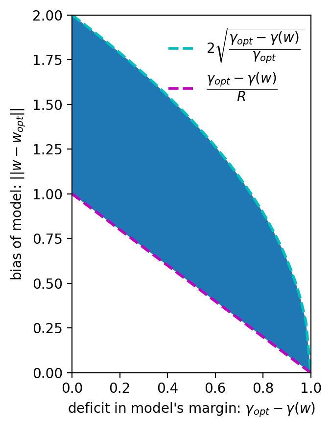
Figure 1: Graphical illustration of (3). For simplicity, the values in on the figure axes assume $\gamma_{opt}=R=1$. The result, developed in Theorem 2.2, states that the plots of the margin deficit versus the bias of the iterates generated by any algorithm must lie within the shaded area. This allows one to transfer convergence rates for the margin to of iterates generated by any optimization algorithm, to convergence rates for the bias and vise versa.

1.2 Related works

There is a rich body of research on understand the limiting dynamics of the iterates generated by gradient-descent, i.e the so-called so-called implicit bias of the latter. In the case of linear models with exponential-tailed losses,  Soudry et al., (2017), Nacson et al., (2018),  Gunasekar et al., (2018),  Ji and Telgarsky, (2019, 2020) make up the standard literature. These papers all prove that the iterates of gradient-descent on linearly separable binary classification problems converge to the max-margin linear classifier ${\mathbf{w}}_{opt}$ with margin $\gamma_{opt}$. They also contain explicit rates of convergence. The very recent work  Ji and Telgarsky, (2020) establishes a convergence rate of $\mathcal{O}(1/t)$ for both the margin the bias of gradient-descent. More precisely, the authors show that gradient-descent on exponentially-tailed loss functions and aggressive stepsizes converges with rate $\mathcal{O}(1/t)$ in both the margin and the bias. These convergence rates are the best known currently in the literature.

Finally, in the case of neural network classifiers, let us mention  Chizat and Bach, (2020) which analyzes gradient-descent on neural networks with one hidden-layer with logistic loss function, and  Lyu and Li, (2020) which studies deep neural networks with positive-homogeneous activation functions (e.g RELU) and exponential-tail loss functions.

2 Main results

2.1 Preliminaries on nonsmooth error bounds

Central to our paper will be the notions of strong slope  De Giorgi et al., (1980) and generalized nonsmooth Kurdyka-Łojasiewicz inequalities  Attouch and Bolte, (2009); Corvellec and Motreanu, (2007); Azé and Corvellec, (2017); Bolte and Blanchet, (2016). These concepts are now standard in optimization. [Nonsmooth Kurdyka-Łojasiewicz inequalites via strong slope] Let $M=(M,d)$ be a complete metric space. An extended-value function $f:M\to\mathbb{R}\cup\{\pm\infty\}$ is said to satisfy a generalized Kurdyka-Łojasiewicz inequality with exponent $\theta>0$ and modulus $\alpha>0$, around the point ${\mathbf{w}}_{0}\in M$ if there exists $\nu>0$ and such that

$$|\partial|^{-}f({\mathbf{w}})\geq\frac{\alpha}{\theta}(f({\mathbf{w}})-f({\mathbf{w}}_{0}))^{1-\theta}\;\forall{\mathbf{w}}\in M\text{ with }f({\mathbf{w}}_{0})<f({\mathbf{w}})<f({\mathbf{w}}_{0})+\nu.$$ (4)

Here, $|\partial|^{-}f({\mathbf{w}})\in[0,+\infty]$ is the strong slope De Giorgi et al., (1980); Corvellec and Motreanu, (2007); Azé and Corvellec, (2017) of $f$ at the point ${\mathbf{w}}$, a ”synthetic” lower-bound of the the rate of change of $f$ at ${\mathbf{w}}$ in any direction, defined by

$$|\partial|^{-}f({\mathbf{w}}):=\limsup_{{\mathbf{w}}^{\prime}\to{\mathbf{w}}}\frac{(f({\mathbf{w}})-f({\mathbf{w}}^{\prime}))_{+}}{d({\mathbf{w}},{\mathbf{w}}^{\prime})}.$$ (5)

Our interest in strong slopes and KL-inequalities is motivated by the following result from  (Azé and Corvellec,, 2017, Corollary 5.1), which will be the main workhorse for proving our theorems. [Nonlinear error-bound via Kurdyka-Łojasiewicz] Let $M$ be a complete metric space and $f:M\to\mathbb{R}\cup\{+\infty\}$ be a proper l.s.c function which satisfies a KL-inequality around ${\mathbf{w}}_{0}$ with exponent $\theta>0$ and other parameters as in (4). Then we have the error bound

$$\operatorname{\sf dist}({\mathbf{w}},\{f\leq f({\mathbf{w}}_{0})\})\geq\frac{(f({\mathbf{w}})-f({\mathbf{w}}_{0}))^{\theta}}{\alpha},\;\forall{\mathbf{w}}\in M\text{ with }f({\mathbf{w}}_{0})<f({\mathbf{w}})<f({\mathbf{w}}_{0})+\nu.$$ (6)

Strong slopes are difficult to compute in general. Fortunately, they can be bounded in terms of more familiar quantities. For example, if $M=(M,\|\cdot\|)$ is a Banach space with topological dual $M^{\star}=(M^{\star},\|\cdot\|_{\star})$ and $\partial f({\mathbf{w}})\subseteq M^{\star}$ is the is the Fréchet subdifferential of $f$ at ${\mathbf{w}}$, defined by

$$\partial f({\mathbf{w}}):=\left\{{\mathbf{w}}^{\star}\in M^{\star}\;\bigg{|}\;\liminf_{{\mathbf{w}}^{\prime}\to{\mathbf{w}}}\frac{f({\mathbf{w}}^{\prime})-f({\mathbf{w}})-\langle{\mathbf{w}}^{\star},{\mathbf{w}}^{\prime}-{\mathbf{w}}\rangle}{\|{\mathbf{w}}^{\prime}-{\mathbf{w}}\|}\geq 0\right\},$$ (7)

then the following bounds hold

$$\liminf_{({\mathbf{w}}^{\prime},f({\mathbf{w}}^{\prime}))\to({\mathbf{w}},f({\mathbf{w}}))}\|\partial f({\mathbf{w}}^{\prime})\|\leq|\partial|^{-}f({\mathbf{w}})\leq\|\partial f({\mathbf{w}})\|_{\star},$$ (8)

where $\|\partial f({\mathbf{w}})\|_{\star}$ is the minimum norm of subgradients of $F$ at ${\mathbf{w}}$, i.e $\|\partial f({\mathbf{w}})\|_{\star}:=\inf\{\|{\mathbf{w}}^{\star}\|_{\star}\mid{\mathbf{w}}^{\star}\in\partial f\}$. See Azé and Corvellec, (2017), for example. In particular,

• If $f$ is convex, then the second inequality in (8) is an equality. In this case, $\partial f$ is given by the familiar formula $\partial f({\mathbf{w}}):=\{{\mathbf{w}}^{\star}\in M^{\star}\mid f({\mathbf{w}}^{\prime})\geq f({\mathbf{w}})+\langle{\mathbf{w}}^{\star},{\mathbf{w}}^{\prime}-{\mathbf{w}}\rangle\;\forall{\mathbf{w}}^{\prime}\in M\}$. Furthermore, if ${\mathbf{w}}$ is not not a local minimum point of $f$, then both inequalities in (8) are equalities.

• If $i_{S}$ is the indicator function of a nonempty subset $S\subseteq M$, then a simple calculation using the definition (7) shows that for every ${\mathbf{w}}\in S$ we have $\partial i_{S}({\mathbf{w}}):=N_{S}^{\text{Fr\'{e}chet}}({\mathbf{w}})$, the Fréchet normal cone of $S$ as ${\mathbf{w}}$, i.e

  $$\partial i_{S}({\mathbf{w}})=N_{S}^{\text{Fr\'{e}chet}}({\mathbf{w}}):=\left\{{\mathbf{w}}^{\star}\in M^{\star}\;\bigg{|}\;\limsup_{{\mathbf{w}}^{\prime}\overset{S}{\to}{\mathbf{w}}}\frac{\langle{\mathbf{w}}^{\star},{\mathbf{w}}^{\prime}-{\mathbf{w}})}{\|{\mathbf{w}}^{\prime}-{\mathbf{w}}\|}\leq 0\right\},$$ (9)

  where ${\mathbf{w}}^{\prime}\overset{S}{\to}{\mathbf{w}}$ is means that the limit is taken ax ${\mathbf{w}}^{\prime}$ tends to ${\mathbf{w}}$ while staying within $S$.

2.2 Statement of main results

The following is the first of our main results. All proofs will be provided in section 3. [Kurdyka-Łojasiewicz inequality for the margin] The extended-value function $f:\mathbb{R}^{m}\to\mathbb{R}\cup\{+\infty\}$ defined by $$f({\mathbf{w}})=\begin{cases}-\gamma({\mathbf{w}}),&\mbox{ if }{\mathbf{w}}\in\mathbb{S}_{m-1},\\ +\infty,&\mbox{ else.}\end{cases}$$ satisfies a KL-inequality (4) around the max-margin model ${\mathbf{w}}_{opt}$, with exponent $\theta=1/2$. Note that the (negative) margin function $-\gamma$ which is the subject of the above theorem is neither smooth nor convex. For our second main contribution, we have the following result. [Bias bounds from margin bounds] For every unit-vector ${\mathbf{w}}\in\mathbb{S}_{m-1}$, we have $\displaystyle\frac{\gamma_{opt}-\gamma({\mathbf{w}})}{R}\leq\|{\mathbf{w}}-{\mathbf{w}}_{opt}\|\leq 2\sqrt{\frac{\gamma_{opt}-\gamma({\mathbf{w}})}{\gamma_{opt}}},$ (10) where $R:=\max_{i\in[n]}\|\mathbf{x}_{i}\|$. [] The above theorem, illustrated in Figure 1, can be used to convert rates of convergence of function values $\gamma({\mathbf{w}}(t))\to\gamma_{opt}$ produced by any algorithm (e.g gradient descent), to rates of convergence of iterates, i.e $\|{\mathbf{w}}(t)-{\mathbf{w}}_{opt}\|\to 0$.

Note that factor $2$ in the RHS of (10) is tight. Indeed consider the classification problem with $n=1$ (just one sample point!), $m=2$, $\mathbf{x}_{1}=(1,0)$ and $y_{1}=1$. The margin of any ${\mathbf{w}}\in\mathbb{S}_{1}$ is $\gamma({\mathbf{w}})=w_{1}$ which is maximized when ${\mathbf{w}}=(1,0)$. Thus, $\gamma_{opt}=1$ and ${\mathbf{w}}_{opt}=(1,0)$. On the other hand, taking ${\mathbf{w}}=(0,1)$, we get $\|{\mathbf{w}}-{\mathbf{w}}_{opt}\|=2$ and $1-\gamma({\mathbf{w}})/\gamma_{opt}=1$ since $\gamma({\mathbf{w}})=0$.

3 Proof of main results

In this section, we will prove our main results, namely Theorem 2.2 and 2.2. Before that, we need some auxiliary results which might be of independent interest themselves.

Notations. Let $\Delta_{n-1}:=\{(q_{1},\ldots,q_{n})\in\mathbb{R}^{n}\mid{\scriptstyle\sum}_{i=1}^{n}q_{i}=1,\min_{i\in[n]}q_{i}\geq 0\}$ be the unit $(n-1)$-dimensional probability simplex. Given a subset $I\subseteq[n]$ of indices, let $\Delta_{n-1}(I):=\{\mathbf{q}\in\Delta_{n-1}\mid{\scriptstyle\sum}_{i\in I}q_{i}=1\}$ be the face of $\Delta_{n-1}$ generated by vertices in $I$. The indicator function $i_{A}$ of a nonempty subset of $\mathbb{R}^{m}$ is the function $i_{A}:\mathbb{R}^{m}\to\mathbb{R}\cup\{+\infty\}$ defined by $i_{A}({\mathbf{w}})=0$ if ${\mathbf{w}}\in A$, and $i_{\mathbb{S}_{m-1}}=+\infty$ else.

[Fréchet subdifferential of negative margin function] The extended-value function $f$ in Theorem 2.2 has Fréchet subdifferential which satisfies the following inclusion

$$\partial f({\mathbf{w}})\subseteq\{b{\mathbf{w}}-{\scriptstyle\sum}_{i=1}^{n}q_{i}y_{i}\mathbf{x}_{i}\mid\mathbf{q}=(q_{1},\ldots,q_{n})\in\Delta_{n-1}(I({\mathbf{w}})),\;b\in\mathbb{R}\}\;\forall{\mathbf{w}}\in{\mathbb{S}_{m-1}},$$

where $I({\mathbf{w}}):=\{i\in[n]\mid y_{i}\mathbf{x}_{i}^{\top}{\mathbf{w}}=\gamma({\mathbf{w}})\}$ is the set of indices of ”support vectors” for ${\mathbf{w}}$.

Proof of Theorem 3.

Let $\mathbf{A}$ be the $n\times m$ matrix with $i$th row $\mathbf{a}_{i}:=-y_{i}\mathbf{x}_{i}$, and observe that we can decompose $f=g+i_{\mathbb{S}_{m-1}}$, where $g:\mathbb{R}^{m}\to\mathbb{R}$ is defined by $g({\mathbf{w}}):=\max_{i\in[n]}g_{i}({\mathbf{w}})$, with $g_{i}({\mathbf{w}}):=\mathbf{a}_{i}^{\top}{\mathbf{w}}$. By the sum-rule for Fréchet subdifferentials, we have $\partial f({\mathbf{w}})\subseteq\partial g({\mathbf{w}})+\partial i_{\mathbb{S}_{m-1}}({\mathbf{w}})$ for all ${\mathbf{w}}\in{\mathbb{S}_{m-1}}$. Also, by a well-known result for the subdifferential of the pointwise maximum of convex functions (e.g see  (Van Ngai et al.,, 2002, Corollary 3.6)), one has

$$\begin{split}\partial g({\mathbf{w}})&=\operatorname{\sf conv}\left(\cup_{i\in I({\mathbf{w}})}\partial g_{i}({\mathbf{w}})\right)=\{{\scriptstyle\sum}_{i=1}^{n}q_{i}{\mathbf{w}}_{i}^{\star}\mid\mathbf{q}\in\Delta_{n-1}(I({\mathbf{w}})),\;{\mathbf{w}}_{i}^{\star}\in\partial g_{i}({\mathbf{w}})\;\forall i\in I({\mathbf{w}})\}\\ &=\{-{\scriptstyle\sum}_{i=1}^{n}q_{i}y_{i}\mathbf{x}_{i}\mid\mathbf{q}\in\Delta_{n-1}(I({\mathbf{w}}))\}=\{\mathbf{A}^{\top}\mathbf{q}\mid\mathbf{q}\in\Delta_{n-1}(I({\mathbf{w}}))\}.\end{split}$$

On the other hand, by (9) and Example 2.6 of  Bauschke et al., (2013), it holds ${\mathbf{w}}\in{\mathbb{S}_{m-1}}$ for all ${\mathbf{w}}\in{\mathbb{S}_{m-1}}$ that $\partial i_{\mathbb{S}_{m-1}}({\mathbf{w}})=\mathbb{R}{\mathbf{w}}:=\{b{\mathbf{w}}\mid b\in\mathbb{R}\}$, the $1$-dimensional subspace of $\mathbb{R}^{m}$ spanned by ${\mathbf{w}}$. Putting things together then gives the result. ∎

For the proof of Theorem 2.2, we will also need the following elementary result (also see  Ji and Telgarsky, (2019)) [] For every $\mathbf{q}=(q_{1},\ldots,q_{n})\in\Delta_{n-1}$, it holds that $\gamma_{opt}\leq\|\sum_{i=1}^{n}q_{i}y_{i}\mathbf{x}_{i}\|\leq 1$. We are now ready to proof Theorem 2.2.

Proof of Theorem 2.2.

Let $f:\mathbb{R}^{m}\to\mathbb{R}\cup\{+\infty\}$ be the negative margin function appearing in the theorem. Thanks to Theorem 3, we know that $\partial f({\mathbf{w}})\subseteq\{\mathbf{A}^{\top}\mathbf{q}+b{\mathbf{w}}\mid\mathbf{q}\in\Delta_{n-1}(I({\mathbf{w}})),\;b\in\mathbb{R}\}$ for all ${\mathbf{w}}\in{\mathbb{S}_{m-1}}$. Thus, we may lower-bound the minimum norm of Fréchet subgradients of $g$ at any point ${\mathbf{w}}\in{\mathbb{S}_{m-1}}$ as follows

$$\begin{split}\|\partial f({\mathbf{w}})\|^{2}&=\inf_{{\mathbf{w}}^{\star}\in\partial f({\mathbf{w}})}\|{\mathbf{w}}^{\star}\|^{2}\geq\inf_{\mathbf{q}\in\Delta_{n-1}(I({\mathbf{w}})),\;b\in\mathbb{R}}\|\mathbf{A}^{\top}\mathbf{q}+b{\mathbf{w}}\|^{2},\text{ by Theorem \ref{thm:frechet}}\\ &=\inf_{\mathbf{q}\in\Delta_{n-1}(I({\mathbf{w}}))}\|\operatorname{\sf P}_{{\mathbf{w}}^{\perp}}(\mathbf{A}^{\top}\mathbf{q})\|^{2},\text{ distance between line and origin}\\ &=\inf_{\mathbf{q}\in\Delta_{n-1}(I({\mathbf{w}}))}\|\mathbf{A}^{\top}\mathbf{q}-({\mathbf{w}}^{\top}\mathbf{A}^{\top}\mathbf{q}){\mathbf{w}}\|^{2},\text{ orthogonal projection formula}\\ &=\inf_{\mathbf{q}\in\Delta_{n-1}(I({\mathbf{w}}))}\|\mathbf{A}^{\top}\mathbf{q}\|^{2}-({\mathbf{w}}^{\top}\mathbf{A}^{\top}\mathbf{q})^{2},\text{ basic linear algebra}\\ &=\inf_{\mathbf{q}\in\Delta_{n-1}(I({\mathbf{w}}))}\|\mathbf{A}^{\top}\mathbf{q}\|^{2}-\gamma({\mathbf{w}})^{2},\text{ because }\mathbf{a}_{i}^{\top}{\mathbf{w}}=-y_{i}\mathbf{x}_{i}^{\top}{\mathbf{w}}=-\gamma({\mathbf{w}})\;\forall i\in I({\mathbf{w}})\\ &\geq\inf_{\mathbf{q}\in\Delta_{n-1}}\|\mathbf{A}^{\top}\mathbf{q}\|^{2}-\gamma({\mathbf{w}})^{2},\text{ since }\Delta_{n-1}(I({\mathbf{w}}))\subseteq\Delta_{n-1}\\ &=\gamma_{opt}^{2}-\gamma({\mathbf{w}})^{2},\text{ by Lemma \ref{lm:smalllemma}}\\ &=(\gamma({\mathbf{w}})+\gamma_{opt})\cdot(-\gamma({\mathbf{w}})+\gamma_{opt})\\ &=(\gamma({\mathbf{w}})+\gamma_{opt})\cdot(f({\mathbf{w}})-\min f),\text{ by definition of }f\\ &\geq\gamma_{opt}\cdot(f({\mathbf{w}})-\min f),\text{ since }\gamma({\mathbf{w}})\geq 0\text{ by assumption}.\end{split}$$

Combining the above inequality with the LHS of (8) then gives

$$|\partial|^{-}f({\mathbf{w}})\geq\liminf_{({\mathbf{w}}^{\prime},f({\mathbf{w}}^{\prime}))\to({\mathbf{w}},f({\mathbf{w}}))}\|\partial f({\mathbf{w}}^{\prime})\|\geq\gamma_{opt}^{1/2}\cdot(f({\mathbf{w}})-\min f)^{1/2}.$$

Thus, the negative margin function $g$ satisfies a KL-inequality around the max-margin model ${\mathbf{w}}_{opt}$, with exponent $\theta=1/2$ and modulus $\alpha=2/\sqrt{\gamma_{opt}}$ as claimed. ∎

Proof of Theorem 2.2.

The LHS of the inequality is trivial since the margin function $\gamma$ is $R$-Lipschitz on $\mathbb{S}_{m-1}$. For the RHS, note from Theorem 2.2 that the negative margin function $g$ (defined in Theorem 2.2) satisfies a KL-inequality around the point ${\mathbf{w}}_{0}={\mathbf{w}}_{opt}$, with exponent $\theta=1/2$ and modulus $\alpha=2/\sqrt{\gamma_{opt}}$. The result then follows as upon invoking Proposition 2.1. ∎

4 Concluding remarks

We have established a Kurdyka-Łojasiewicz inequality with exponent $1/2$ for the margin function in linearly separable classification problems. This result gives hopes for the existence of fast (perhaps quasi-linear) optimization schemes for such problems, a quest which will be pursued in future work. Also, we have employed our result to establish a generic inequality linking the convergence rates of the bias and of margin. This immediately allows for the transfer of convergence rates for the margin, to convergence rates for the bias, irrespective of the algorithms / constructs (gradient-flow, gradient-descent, what stepsize, etc.) used to establish the former.

Acknowledgement.

The author is thankful to Ziwei Ji and Matus Telgarsky for reporting an error in one of the theorems in an earlier version of this preprint. Also, thanks to Eugene Ndiaye for proof-reading the manuscript.

Appendix A Omitted technical proofs

See 3

Proof.

For any $\mathbf{q}=(q_{1},\ldots,q_{n})\in\Delta_{n-1}$, one computes

$$\begin{split}\|\sum_{=1}^{,}q_{i}y_{i}\mathbf{x}_{i}\|&=\sup_{\mathbf{u}\in\mathbb{B}_{M}}\langle\sum_{i=1}^{n}q_{i}y_{i}\mathbf{x}_{i},\mathbf{u}\rangle=\sup_{\mathbf{u}\in\mathbb{B}_{M}}\mathbb{E}_{i\sim\mathbf{q}}[y_{i}\langle\mathbf{x}_{i},\mathbf{u}\rangle]\\ &\geq\mathbb{E}_{i\sim\mathbf{q}}[y_{i}\langle\mathbf{x}_{i},{\mathbf{w}}^{\text{opt}}_{n}\rangle],\text{ by taking any }\mathbf{u}={\mathbf{w}}_{n}^{\text{opt}}\in\operatorname{\sf OPT}_{n}\\ &\geq\gamma_{opt},\text{ by definition of }\gamma_{opt}.\end{split}$$

This proves the lower-bound. On the other hand, using the fact that

$$\sup_{\mathbf{u}\in\mathbb{B}_{M}}\mathbb{E}_{i\sim\mathbf{q}}[y_{i}\langle\mathbf{x}_{i},\mathbf{u}\rangle]\leq\mathbb{E}_{i\sim\mathbf{q}}[\sup_{\mathbf{u}\in\mathbb{B}_{M}}y\langle\mathbf{x}_{i},\mathbf{u}\rangle]=\mathbb{E}_{i\sim\mathbf{q}}[\|\mathbf{x}\|]\leq 1,$$

since $\|\mathbf{x}_{i}\|\leq 1$ for all $i\in[n]$ by hypothesis. This proves the upper-bound. ∎

References

• Attouch and Bolte, (2009) Attouch, H. and Bolte, J. (2009). On the convergence of the proximal algorithm for nonsmooth functions involving analytic features. Mathematical Programming, 116(1).
• Azรฉ and Corvellec, (2017) Azรฉ, D. and Corvellec, J.-N. (2017). Nonlinear error bounds via a change of function. Journal of Optimization Theory and Applications, 172.
• Bauschke etย al., (2013) Bauschke, H.ย H., Luke, D.ย R., Phan, H.ย M., and Wang, X. (2013). Restricted normal cones and the method of alternating projections: Applications. Set-Valued and Variational Analysis, 21(3).
• Bolte and Blanchet, (2016) Bolte, J. and Blanchet, A. (2016). A family of functional inequalities: Lojasiewicz inequalities and displacement convex functions. arXiv e-prints.
• Chizat and Bach, (2020) Chizat, L. and Bach, F. (2020). Implicit bias of gradient descent for wide two-layer neural networks trained with the logistic loss. In Conference on Learning Theory, COLT 2020, 9-12 July 2020, Virtual Event [Graz, Austria], volume 125 of Proceedings of Machine Learning Research. PMLR.
• Corvellec and Motreanu, (2007) Corvellec, J.-N. and Motreanu, V.ย V. (2007). Nonlinear error bounds for lower semicontinuous functions on metric spaces. Mathematical Programming, 114(2):291.
• De Giorgi etย al., (1980) De Giorgi, E., Marino, A., and Tosques, M. (1980). Problemi di evoluzione in spazi metrici e curve di massima pendenza. Atti della Accademia Nazionale dei Lincei. Classe di Scienze Fisiche, Matematiche e Naturali. Rendiconti, 68(3):180โ€“187.
• Gunasekar etย al., (2018) Gunasekar, S., Lee, J., Soudry, D., and Srebro, N. (2018). Characterizing Implicit Bias in Terms of Optimization Geometry. arXiv e-prints, page arXiv:1802.08246.
• Ji and Telgarsky, (2019) Ji, Z. and Telgarsky, M. (2019). A refined primal-dual analysis of the implicit bias. arXiv:1906.04540 (version v1 of manuscript).
• Ji and Telgarsky, (2020) Ji, Z. and Telgarsky, M. (2020). Characterizing the implicit bias via a primal-dual analysis. arXiv:1906.04540 (version v2 of manuscript).
• Lyu and Li, (2020) Lyu, K. and Li, J. (2020). Gradient descent maximizes the margin of homogeneous neural networks. In 8th International Conference on Learning Representations, ICLR 2020. OpenReview.net.
• Nacson etย al., (2018) Nacson, M., Lee, J.ย D., Gunasekar, S., Savarese, P. H.ย P., Srebro, N., and Soudry, D. (2018). Convergence of Gradient Descent on Separable Data. arXiv e-prints, page arXiv:1803.01905.
• Soudry etย al., (2017) Soudry, D., Hoffer, E., Shpigel Nacson, M., Gunasekar, S., and Srebro, N. (2017). The Implicit Bias of Gradient Descent on Separable Data. arXiv e-prints, page arXiv:1710.10345.
• Van Ngai etย al., (2002) Van Ngai, H., The Luc, D., and Thรฉra, M. (2002). Extensions of frรฉchet $\epsilon$-subdifferential calculus and applications. Journal of Mathematical Analysis and Applications, 268(1).