Quantitative reinterpretation of quartz-crystal-microbalance experiments with adsorbed particles using analytic hydrodynamics

Abstract

Despite being a fundamental tool in soft matter research, quartz crystal microbalance (QCM) analyses of discrete macromolecules in liquid so far lack a firm theoretical basis. Currently, acoustic signals are qualitatively interpreted using ad-hoc frameworks based on effective electrical circuits, effective springs and trapped-solvent models with abundant fitting parameters. Nevertheless, due to its extreme sensitivity, the QCM technique pledges to become an accurate predictive tool. Using unsteady low Reynolds hydrodynamics we derive analytical expressions for the acoustic impedance of adsorbed discrete spheres. Our theory is successfully validated against 3D simulations and a plethora of experimental results covering more than a decade of research on proteins, viruses, liposomes, massive nanoparticles, with sizes ranging from few to hundreds of nanometers. The excellent agreement without fitting constants clearly indicates that the acoustic response is dominated by the hydrodynamic impedance, thus, deciphering the secondary contribution of physico-chemical forces will first require a hydrodynamic-reinterpretation of QCM.

I Introduction

The quartz crystal microbalance (QCM) is one of the most versatile tools to study subtle effects in soft matter, resolving forces in the pico-Newton to nano-Newton range and nano-gram masses. Due to its low operating cost, sensor compactness, real-time data, label-free operation and subnanogram sensitivity, QCM has become a fundamental tool in analytical chemistry and biophysics research. The number of applications (from nanotribology to health care, environmental monitoring [1, 2, 3, 4] and even crude oil [5]) is huge and cannot be exhaustively listed here. QCM has also become one of the important techniques in biosensing for DNA [6, 7, 8, 9] and other biomolecules [10] including virus detection [11]. These distinct features make QCM competitive with other common analytical and detection tools [12] such as optical DNA detection via fluorescence-labeled oligonucleotides, surface plasmon resonance [13], or electrochemical assays. Subtle nanometric phenomena such as variations in contact forces, molecular stiffness [14, 15], kinetics of adsorption or bio-molecular interactions [16] are routinely sensed using QCM. However, in these liquid environments, QCM lacks the theoretical foundation required to become a measurement technique.

The idea of using the inverse piezoelectric effect to sense mass, which is in essence the QCM, was born for experiments in a vacuum. The surface of a cut of crystal quartz exposed to an AC potential, oscillates at MHz frequency and the inertia of tiny amounts of deposited material creates a detectable reduction in the oscillation frequency $\Delta f<0$. Sauerbrey [17] converted this phenomenon into a mass balance, by showing the proportionality between $-\Delta f$ and the deposited mass per unit surface $m_{\mathrm{QCM}}$,

$$m_{\mathrm{QCM}}=-\mathrm{C}\Delta f/n$$ (1)

where $n$ is the overtone of the surface wave (odd integer $n\leq 13$). The mass sensitivity constant, typically $\mathrm{C=17.7\ \mathrm{ng}\cdot\mathrm{cm}^{-2}\mathrm{Hz}^{-1}}$, reveals an extremely small limit of detection, as $\Delta f\sim-0.1\ \mathrm{Hz}$ represents $1.7\ \mathrm{ng/cm^{2}}$.

Interpreting QCM in liquids faced challenges, many of them still unresolved. In a liquid, viscous forces propagate the wall oscillation upwards, moving a layer of fluid of about 3 times the so-called penetration depth $\delta=(2\eta/\rho\omega)^{1/2}$ (here $\omega=2\pi f$, $\eta$ is the fluid viscosity and $\rho$ its density). In water, $\delta\propto\eta^{-1/2}$ typically ranges from 71 to 238 nm. The resulting laminar flow, called Stokes flow, creates wall viscous stress oscillating with a $45^{o}$ phase lag with respect the surface motion. The out-of-phase component damps the wall motion. Its decay rate $2\pi\Gamma$ is directly measured in “ring-down” sensors (QCM-D) [2] while in forced QCM, this dissipative effect broadens the spectra, with half bandwidth $\Gamma$ and quality factor $f/(2\Gamma)$. The new actor, “dissipation” $D=2\Gamma/f$, introduces another channel of information in liquids. In Newtonian fluids [18, 19] $-\Delta f$ and $\Delta\Gamma$ are equal and proportional to the mass of moving fluid. Viscoelastic films [20, 21] present different contributions which can be traced using 1D laminar flow equations. However, QCM was soon used to investigate all sorts of soft discrete 3D objects, for which an analytical approach has so far been elusive. The QCM technique faced proteins [22, 23], DNA strands [24], supported lipid bilayers [25, 26, 27], polymers [28], vesicles [29], liposomes [30, 8, 9], viruses [31, 11], different kinds of nano and microparticles [32, 6, 7, 10], bacteria [14], living cells [33], crude oil [5] and more.

Experiments urgently required ways to rationalize the distinct acoustic features and peculiar behaviors of these discrete analytes. The adsorbed mass predicted from $\Delta f$ using Eq. 1 was seen to significantly differ (usually appearing larger) than other independent measurements of $m$, e.g. using scanning electron microscopy (SEM) [34, 35]. For more than one decade such a difference, measured by the mass ratio $H=1-m/m_{\mathrm{QCM}}$ [34, 36, 37], has been explained using the “trapped solvent” model [34] which assumes that the extra QCM mass is due to solvent molecules being trapped by the analyte and moving concomitantly with it. Despite the reported deficiencies [35], several versions of this model are still routinely used to interpret experiments [37].

Another unexplained puzzling phenomenon concerns the frequency inversion. As the analyte size (or QCM frequency) is increased, $\Delta f$ becomes more and more negative until above a certain size (or frequency) it suddenly becomes positive [38]. Phenomenological models were designed to reproduce such behavior. The coupled-resonator model [39] is based on a series of masses connected with effective springs representing analyte-wall contacts [40, 39, 41, 2] placed either in parallel (Kelvin-Voight) or in series (Maxwell model) [14]. This model predicts a transition from “inertial” ($\Delta f<0$) to “elastic” ($\Delta f>0$) response at high frequency, when the large contact stiffness overpowers the inertia of deposited mass. Imaginary springs are also added to act as dampers, introducing the concept of “viscous load” ($\Delta\Gamma>0$) of the adsorbed structure. Tuning the model parameters permits fitting experimental data and gauging different analyte “stiffnesses”, adsorbed “mass” or analyte-wall “interactions”. However, the coupled-resonator model completely neglects the role of the solvent hydrodynamics. These phenomenological pictures very much constitute the basis of present analyses [15, 14]. Quoting Tarnapolsky and Freger [41], QCM-D has “mainly become a comparative tool in particle adhesion research. Unfortunately, such development lacks an adequate quantitative model”.

About one decade ago, simulations started to highlight the relevance of hydrodynamics in discrete-particle QCM [31, 42]. Coverage effects such as the decrease of the acoustic ratio $-\Delta D/\Delta f$ with $\Delta f$ were qualitatively reproduced in 2D simulations [31, 42] and later in 3D [43, 44], revealing a hydrodynamic origin, which has not yet been theoretically explained. The relevance of the particle shape [45] was also analyzed. Recently, it was proved that hydrodynamics lie behind the extreme sensitivity of QCM to how broadly mass is distributed over the resonator [9] and also that it is responsible for anti-Sauerbrey responses ($\Delta f>0$) [38].

Before introducing the concept of hydrodynamic impedance, a comment on the phasor formalism is in order. The resonator position can be expressed as $\tilde{x}(t)=\mathrm{Re}[x\,\exp(-\mathrm{i}\hat{\omega}t)]$ where $\hat{\omega}\equiv 2\pi f-\mathrm{i}2\pi\Gamma$ is the complex frequency and $x$ is its phasor (note that $\Gamma>0$ implies an exponential decay). This complex number determines its phase lag with respect some time reference. The central phasor quantity in QCM is the impedance $\mathrm{Z}=\overline{\sigma_{\mathrm{wall}}}/\mathrm{v}_{0}$ which, following the small load approximation ($\Delta f/f<<1$), relates the overall tangential wall-stress $\overline{\sigma_{\mathrm{wall}}}\equiv\hat{\bf x}\cdot\overline{\boldsymbol{\sigma}_{\mathrm{wall}}}\cdot\hat{\bf z}$ with the complex frequency shift [2],

$$\Delta f-\mathrm{i}\Delta\Gamma=\mathrm{i}f\frac{\mathrm{Z}}{\pi\mathrm{Z}_{Q}},$$ (2)

where the impedance of the quartz crystal cut is usually $\mathrm{Z}_{Q}=8.8\times 10^{6}\ \mathrm{kg/(m^{2}s)}$.

The origin of the hydrodynamic impedance is simple [9, 38]: any force acting on the analyte propagates fluid momentum to the resonator, creating extra wall-stress which is measured by the QCM. It is important to note that particle-forces arise not only from molecular linkers, adhesion forces, etc., but they are also induced by the fluid traction itself. In fact, we shall show that the QCM response is dominated by fluid-induced forces. In any case, to understand the QCM response one needs to determine the lag-time required to transmit the analyte-force to the wall. This time crucially depends on the vertical coordinate $z$ because (as shown below) the fluid-momentum propagator is proportional to $\exp(-\alpha z)$, with $\alpha=(1-\mathrm{i})/\delta$. Without loss of generality, let the wall phasor $x=x_{0}$ be a real number and consider an oscillatory force in phase with the wall ($F$ is real), acting at some point located at $z=d$. This force transfers a hydrodynamic stress $(F/A)\exp(-\alpha d)$ to the wall ($A$ is the resonator area) creating an impedance $Z=[F/(A\omega x_{0})]\mathrm{i}\exp[-\alpha d]$. If the force is placed at the wall ($d=0$) this leads to $\mathrm{Re}[\mathrm{Z}]=0$ and $\mathrm{Im}[\mathrm{Z}]>0$ (or, from Eq. 2, $\Delta\Gamma=0$ and $\Delta f<0$). In the QCM jargon this would correspond to an inertial load. But the very same force applied at $d=(\pi/2)\delta$ would then be understood as a purely viscous load ($\Delta\Gamma>0$ and $\Delta f=0$), while farther away it would become an elastic load ($\Delta f>0$). This simple example clearly illustrates the need for a rigorous hydrodynamic reinterpretation of QCM signals.

In general, the values of $\Delta f$ and $\Delta\Gamma$ result from summing up the propagation of all forces acting on each point of the ensemble of analytes. This leads to a far-from-trivial convolution expression, which should be derived using zero-Reynolds unsteady hydrodynamics [46, 47, 48]. Indeed, the hydrodynamics of QCM gathers all the difficulties one might expect: the semi-bounded unsteady flow lacks spherical symmetry and obtaining the perturbative flow created by the particle (which creates the extra wall stress) requires solving the dynamics of the analyte, which, in turn, is coupled to the fluid-induced forces. While such an intertwined problem can be partially tackled in the case of point particles [49], many QCM analytes (liposomes, nanoparticles) are far from being “points” and reach the size of the penetration depth $R\sim\delta\sim 100\mathrm{nm}$. Fortunately, QCM senses the total stress over the surface which simplifies the analytical expressions for the impedance of finite adsorbed particles, derived below. Comparison with 3D simulations and abundant available experimental data proves that our approach is valid up to $R/\delta<2$. Notably, although we just consider free particles (wall-particle forces are absent) the theory shows an excellent agreement with quite a disparate set of experiments, without any fitting constants. This result urgently calls for a quantitative reinterpretation of QCM signals starting from the dominant role of hydrodynamics, adding to the predictive power of QCM and becoming a tool for measuring relevant forces, due to molecular/structural elasticity, adhesion, ionic-strength or other long-ranged physico-chemical interactions with the substrate.

II Results

II.1 Theory

We consider a sphere of radius $R$ and density $\rho_{p}$ whose center, located at ${\bf r}_{c}=(0,0,d)$, is at distance $d$ from the QCM plane $z=0$. The QCM resonator oscillates at angular frequency $\omega$ in the $x$ direction with velocity $\mathrm{v}_{0}\,\cos(\omega t)$ and its amplitude $x_{0}$ is small enough (typically around $2\mathrm{nm}$) to neglect non-linear couplings. The total impedance $\mathrm{Z}$ sums up all the forces (per area) acting on the surface. As customary, the baseline is set at the impedance of the base Stokes flow (equal to $\eta\alpha$) so we consider stress in excess of that reference. The forces acting on the wall are either directly due to the particle (impedance noted as $\mathrm{Z}_{\mathrm{pw}}$) or to the fluid (hydrodynamic impedance, $\mathrm{Z}_{\mathrm{hydro}}$),

$$\mathrm{Z}=\mathrm{Z}_{\mathrm{pw}}+\mathrm{Z}_{\mathrm{hydro}}$$ (3)

In turn, $\mathrm{Z}_{\mathrm{pw}}$ has contributions from the particle inertia and from wall-particle forces (adhesion, molecular linkers, etc.). The latter will not be considered hereafter, so as to isolate the hydrodynamic effects. The particle inertia is just the Archimedean force due to the acceleration of the excess particle mass so that $\mathrm{Z}_{\mathrm{pw}}=\mathrm{i}nm_{e}\omega$. Implicitly, we have assumed that the adsorbed particle velocity $u$ concomitantly follows that of the resonator $u=\mathrm{v}_{0}$. Here $n$ is the particle’s surface density and $m_{e}=(\rho_{p}-\rho)V_{p}$ is the excess in mass with respect to the displaced fluid ($V_{p}=4\pi R^{3}/3$ is the particle volume). In terms of the scaled impedance $\hat{\mathcal{Z}}_{\mathrm{pw}}\equiv\mathrm{Z}_{\mathrm{pw}}/(6\pi\eta nR)=-(2/9)(\rho_{e}/\rho)(\alpha R)^{2}$, with $\rho_{e}=\rho_{p}-\rho$. This is precisely the Sauerbrey contribution to the impedance, with zero dissipation and negative frequency shift (i.e, $\mathrm{Re}[Z_{\mathrm{pw}}]=0$ and $\mathrm{Im}[Z_{\mathrm{pw}}]>0$, as $\mathrm{Im}[\alpha^{2}]<0$).

Any force acting on the particle is transferred back to the fluid (Newton’s third law) as a force density field which propagates momentum to the surface and creates extra wall-stress (detected by the QCM device as frequency $\Delta f$ and dissipation $\Delta D$ shifts). As stated, here we will only consider fluid-induced forces. The fluid velocity field can be expressed as ${\bf v}={\bf v}_{\infty}+{\bf v}_{p}$, where ${\bf v}_{p}$ is the perturbative flow created by the particle presence and the ambient flow $v_{\infty}$ is here ascribed to the base laminar Stokes profile ${\bf v}_{\infty}={\bf v}_{S}=v_{s}(z){\hat{{\bf x}}}$. Its phasor satisfies $v_{s}^{\prime\prime}-\alpha^{2}v_{s}=0$ (prime denotes spatial derivation) with boundary conditions $v_{s}(0)=\mathrm{v}_{0}$ and $v_{s}(\infty)=0$. The solution, $v_{s}(z)=\mathrm{v}_{0}\,\exp(-\alpha z)$, unveils the exponential propagator of momentum mentioned above.

The hydrodynamic impedance requires evaluating the tangential stress due to the perturbative flow at the resonator $z=0$. Such a flow is governed by the Green function tensor field $\boldsymbol{\mathrm{G}}({\bf r},{\bf r}^{\prime})$ of the problem (Methods). For instance, a point-particle at ${\bf r}_{c}$ receiving an oscillatory force (phasor) $-{\bf F}$ creates a flow field ${\bf v}_{p}({\bf r})=\boldsymbol{\mathrm{G}}({\bf r},{\bf r}_{c}){\bf F}$. A finite particle propagates the forces acting on each differential element $dS^{\prime}$ on its surface, which (in the absence of wall or external forces) is induced by the fluid pressure at the particle surface, so

$${\bf v}_{p}({\bf r})=\oint\boldsymbol{\mathrm{G}}({\bf r},{\bf r}^{\prime})\boldsymbol{\Pi}({\bf r}^{\prime})\cdot\hat{{\bf n}}dS^{\prime}.$$ (4)

Here $\boldsymbol{\Pi}({\bf r}^{\prime})$ is the local fluid pressure tensor, $\hat{{\bf n}}$ is the outwards surface vector and the integral runs over the particle surface with $dS^{\prime}$ centered at ${\bf r}^{\prime}$. As ${\bf v}_{S}(z=0)=\mathrm{v}_{0}$, one has to impose ${\bf v}_{p}=0$ at $z=0$ and at $z\rightarrow\infty$; these boundary conditions are inherited by $\boldsymbol{\mathrm{G}}({\bf r},{\bf r}^{\prime})$ (see Methods). In the present setup, however, an explicit derivation of ${\bf v}_{p}$ faces serious difficulties. The Faxén theorem route consists in integrating the no-slip condition ${\bf v}={\bf u}$ at the particle surface to impose a translational (and in general rotational) constraint $\overline{{\bf v}}^{(s)}\equiv\oint{\bf v}dr^{2}/(4\pi R^{2})={\bf u}$ onto Eq. 4. Providing ${\bf u}$ should lead to $\boldsymbol{\Pi}$. In general, though, ${\bf u}$ for suspended particles has to be determined from the particle equation of motion (for a free particle, $-\mathrm{i}m_{p}\omega{\bf u}=\oint\boldsymbol{\Pi}({\bf r})\cdot\hat{{\bf n}}dS$). Due to the lack of spherical symmetry this route becomes impracticable and, to complicate matters further, in this setup $\boldsymbol{\mathrm{G}}({\bf r},{\bf r}^{\prime})$ has no closed analytical form[47]. A second route, based on hydrodynamic reflections [46, 49] is to expand $\boldsymbol{\Pi}$ into ambient and perturbative parts $\boldsymbol{\Pi}=\boldsymbol{\Pi}_{S}+\boldsymbol{\Pi}_{p}$. Introducing this form into Eq.4 leads to a series expansion with operators acting on ${\bf v}_{s}$ and involving increasing powers of $\boldsymbol{\mathrm{G}}$. But again, this requires a closed form for $\boldsymbol{\mathrm{G}}$ in real space. Fortunately, Felderhof [48] demonstrated that it is possible to derive the Fourier transform of $\boldsymbol{\mathrm{G}}({\bf r},{\bf r}^{\prime})$ in the xy-plane which, as we will show shortly, suffices for our purposes. The pressure tensor has a viscous stress $\boldsymbol{\sigma}$ and a kinetic pressure contribution which create a viscous $Z_{v}$ and kinetic $Z_{k}$ impedance derived below. The kinetic stress is just the virial pressure created by fluid inertial forces relative to the base flow $\mathrm{i}\omega(\rho_{p}{\bf u}-\rho\overline{{\bf v}_{s}}^{(v)})$ (with $\overline{{\bf v}_{s}}^{(v)}=[3/(4\pi R^{3})]\int{\bf v}({\bf r})d^{3}r$ the average fluid velocity over the particle volume). The viscous stress includes a dominant contribution from the Stokes base flow $\boldsymbol{\sigma}_{S}$ and another from the perturbative flow $\boldsymbol{\Pi}_{p}$. The excess pressure tensor at the particle surface can thus be written as ,

$$\boldsymbol{\Pi}({\bf r}^{\prime})=\boldsymbol{\sigma}_{S}({\bf r}^{\prime})+\mathrm{i}\omega\left(\rho_{p}{\bf u}-\rho\overline{{\bf v}_{s}}^{(v)}\right){{\bf r}^{\prime}}+\boldsymbol{\Pi}_{p},$$ (5)

where $\boldsymbol{\sigma}_{S}=\eta v_{S}^{\prime}(z)\hat{\bf x}\hat{\bf z}$ and $\boldsymbol{\Pi}_{p}$ is expected to be small for $R/\delta<O(1)$ and shall be neglected in this analysis. This approximation finds support later in the comparison to simulations and experimental results. We assume that the particle moves in the $x$ direction ${\bf u}=u\hat{\bf x}$ and note that $\overline{{\bf v}_{s}}^{(v)}=\overline{v_{s}}^{(v)}\hat{{\bf x}}$.

To evaluate the net shear stress at the wall, one needs to integrate over the resonator plane ($z=0$), the tangential stress $\eta\partial_{z}{\bf v}_{p}\cdot\hat{{\bf x}}$ due to the perturbative flow in Eq. 4,

$$\overline{\sigma_{\mathrm{wall}}}=n\eta\int_{z=0}dS\,\oint_{r=a}\hat{{\bf x}}\cdot\left[\partial_{z}\boldsymbol{\mathrm{G}}({\bf r},{\bf r}^{\prime})\right]_{z=0}\boldsymbol{\Pi}\cdot{\hat{\bf n}}\,dS^{\prime}$$ (6)

Owing to the planar symmetry of the system [48] $\boldsymbol{\mathrm{G}}({\bf r},{\bf r}^{\prime})=\boldsymbol{\mathrm{G}}({\bf s}-{\bf s}^{\prime};z,z^{\prime})$ where ${\bf r}={\bf s}+z\hat{\bf k}$ and ${\bf s}$ lies on the xy-plane. This permits the introduction of the Fourier transform on the xy-plane,

$$\boldsymbol{\mathrm{G}}({\bf s}-{\bf s}^{\prime},z,z^{\prime})=\int d{\bf q}e^{\mathrm{i}{\bf q}\cdot({{\bf s}}-{{\bf s}^{\prime}})}\hat{\boldsymbol{\mathrm{G}}}({\bf q},z,z^{\prime})$$

to obtain

$$\overline{\sigma_{\mathrm{wall}}}=\\ n\eta\int_{z=0}d^{2}{\bf s}\oint_{r=a}dS^{\prime}\int d{\bf q}e^{\mathrm{i}{\bf q}\cdot({{\bf s}}-{{\bf s}^{\prime}})}\hat{{\bf x}}\cdot\partial_{z}\boldsymbol{\mathrm{\hat{G}}}({\bf q},z;z^{\prime})\boldsymbol{\Pi}\cdot{\hat{\bf n}}.$$ (7)

Using the Dirac delta relation $\int\exp(-\mathrm{i}{\bf q}\cdot{{\bf s}})ds^{2}=4\pi^{2}\delta({\bf q})$,

$$\overline{\sigma_{\mathrm{wall}}}=4\pi^{2}n\eta\oint_{r=a}\lim_{q\rightarrow 0}\hat{{\bf x}}\cdot\left[\partial_{z}\boldsymbol{\mathrm{\hat{G}}}(q,z;z^{\prime})\right]_{z=0}\boldsymbol{\Pi}\cdot{\hat{\bf n}}dS^{\prime}$$ (8)

Taking the $q\rightarrow 0$ limit in the full expression for $\partial_{z}\boldsymbol{\mathrm{\hat{G}}}(q,z,z^{\prime})$ at $z=0$ (see Ref. [50]) leads to a particularly simple expression. For the relevant $xx$ component,

$$\lim_{q\rightarrow 0}\partial_{z}\mathrm{\hat{G}}_{xx}(q,z=0;z^{\prime})=-\frac{\exp[-\alpha z^{\prime}]}{4\pi\eta}$$

This allows us to integrate Eq. 8 and derive the impedance due to the viscous stress $\boldsymbol{\sigma}_{S}$ in 5,

$$\hat{\mathcal{Z}}_{v}(d,R)\equiv\frac{Z_{v}}{6\pi n\eta R}=-\frac{\pi e^{-2\alpha d}}{6}\left(\frac{2\alpha R\cosh(2\alpha R)-\sinh(2\alpha R)}{\alpha R}\right)$$ (9)

and the kinetic contribution,

$$\hat{\mathcal{Z}}_{k}(d,R)=\\ -\frac{2\pi}{3}\frac{e^{-\alpha d}}{\alpha R}\left(\alpha R\cosh(\alpha R)-\sinh(\alpha R)\right)\left(\frac{\rho_{p}u-\rho\overline{v_{s}}^{(v)}}{\rho\mathrm{v}_{0}}\right).$$ (10)

These expressions apply for a particle suspended at a distance $d$ over the resonator, moving with a velocity $u$ (in turn, $u$ needs to be determined from the flow-traction, see SI). To evaluate the impedance of adsorbed particles $Z^{(ad)}$ we set $d=R$ and $u=\mathrm{v}_{0}$ and add the Sauerbrey contribution, leading to

$$\hat{\mathcal{Z}}^{(ad)}(R)=-\frac{2\rho_{e}}{9\rho}(\alpha R)^{2}+\hat{\mathcal{Z}}_{v}(R,R)+\hat{\mathcal{Z}}_{k}(R,R)+\hat{\mathcal{Z}}_{p}\;\;\textrm{ (with }u=\mathrm{v}_{0}\textrm{)}.$$ (11)

Recall that we neglect the impedance due to the perturbative flow $\hat{\mathcal{Z}}_{p}$ and later validate such an approximation. It is interesting to scrutinize the robustness of the “no-slip” condition $u=\mathrm{v}_{0}$ to estimate how feasible it is to get a phase lag between $u$ and $\mathrm{v}_{0}$. To this end Fig. 1 illustrates the velocity of a free sphere moving at a gap-distance $\Delta=d-R$ over the oscillating surface. The case corresponds to $R=50\ \mathrm{nm}$. Solid lines correspond to the Mazur-Bedeaux relation [51] (see SI), which is valid far away from the surface, as it neglects the reaction field reflected back from the wall. Notably, even in the absence of wall-particle forces, the strong hydrodynamic friction close to the wall (lubrication) leads to $u\approx\mathrm{v}_{0}$ as $\Delta\rightarrow 0$ (we note that particle slip might take place in specific cases, for instance between two smooth hydrophilic surfaces [52]). If the fluid carries along the particle concomitantly with the wall, the amplitude of any (distance-dependent) wall-particle force should be small or even zero, thus creating a small load impedance. This fact partially explains why the present theory reproduces so well a large list of experiments with considerably different colloidal particles and substrates.

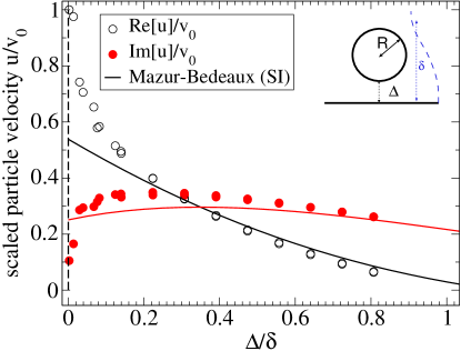
Figure 1: Translational velocity of a spherical particle of radius $R=50\ \mathrm{nm}$ suspended over the QCM surface. The distance $\Delta=d-R$ is the gap between the particle surface and the QCM surface, and $\delta$ is the Stokes flow penetration length. Dashed lines correspond to the result of Mazur and Bedeaux relation [51] (see Supplementary Information) taking the Stokes flow as the mean flow.

In what follows we compare the prediction in Eq. 11 with 3D simulations of spherical rigid particles (Methods) and with published experimental data for a wide range of analytes. We first deal with quasi-neutrally buoyant analytes (proteins, viruses, liposomes, polymer beads) which possess densities $\rho_{p}$ that differ from that of the solvent by less than $30\%$ and also treat their mixtures (latex nanoparticles [53]). Secondly, we consider inertial effects in massive particles by comparing the present theory with experiments with silica nanoparticles in ethanol $\rho_{p}\approx 2.42\rho$ [54].

II.2 Neutrally buoyant particles

II.2.1 Comparison with simulations

Simulations of neutrally buoyant spheres ($\rho_{p}=\rho$ in Eq. 10 and $\rho_{e}=0$ in Eq. 11) were performed using the immersed boundary method combined with an elastic network model for rigid spheres. Details can be found in [9] and Methods. We measured the impedance as a function of the resonator-particle gap distance $\Delta$ [9] and here we consider the limit $\Delta\rightarrow 0$, to deal with the case of adsorbed particles. Again, it is important to stress that in these simulations we have not imposed any adhesion force between the particle and the wall, so their impedance arises only from purely hydrodynamic effects [38].

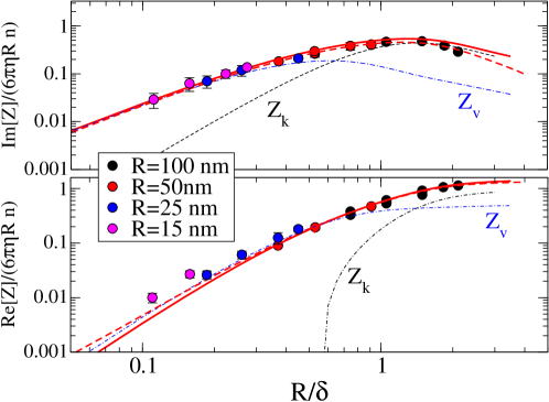
Figure 2: Scaled impedances comparing simulations and the theoretical result in Eq. 11 (solid lines). Dashed lines correspond to $Z_{v}$ (Eq. 9) and $Z_{k}$ (10), as indicated.

Figure 2 compares the prediction in Eq. 11 with simulation results. The agreement is excellent, both for the real and the imaginary parts of $Z$. Figure 2 shows the contributions to the hydrodynamic impedance in Eq. 11. The viscous contribution $Z_{v}$ dominates the impedance of small particles $R/\delta<0.5$. Contrary to the commonly assumed relation between viscous forces and dissipation, $Z_{v}$ determines both $\Delta f$ and $\Delta D$ for small $R$. In turn, for large particles $R\gtrsim\delta$, the inertia of the displaced fluid $Z_{k}$ becomes dominant (although $\mathrm{Re}[Z_{v}]$ remains significant). A maximum of $\mathrm{Im}[Z]$ is found near $R/\delta\approx 1.5$, which corresponds to the most negative value of $\Delta f$. For $R/\delta>2$ (not shown) a sudden transition to $\mathrm{Im}[Z]<0$ ($\Delta f>0$) is expected [38, 40, 41]). Interestingly, Eq. 11 predicts the cross-over, but just for any non-zero gap $\Delta>0$. This suggests that the frequency inversion could be consequence of the counter-flow created by the near-field perturbative current and possibly some particle velocity phase-lag induced by slip or rotation about the linker point [41]. The analysis of this range of $R/\delta$ is left for a future contribution.

Table 1: List of experiments analyzed in this work, including the material (liposomes, viruses, proteins…), the radius of the particle and the reported frequency range. Soft^∗ liposomes (DMPC at $32^{o}\mathrm{C}$) deform upon adsorption and their diameter in bulk fluid is larger than the height $h$ they expose over the surface. The given value is $h/2$, rather than the liposome radius in bulk (which is about 60 nm [30]). The substrate b-SLB means biotinylated supported lipid bilayers.

Material	Particle radius [nm]	Frequency range [MHz]	Label	Reference
Rigid liposome DPPC	$57\pm 4$	$[15-75]$	DPPC-57 2009	[31]
Rigid liposome DPPC	$41\pm 2$	$[15-75]$	DPPC-41 2009	[31]
Cow Pea Mosaic Virus (CPMV)	$14$	$[15-75]$	CPMV-14 2009	[31]
Rigid liposome DPPC at $25^{o}C$	$41.5$	$[15-75]$	DPPC-41 2012	[30]
Rigid liposome DMPC at $10^{o}C$	$45$	$[15-55]$	DMPC-45 2012	[30]
Soft∗ liposome DMPC at $32^{o}C$	$33$	$[15-55]$	DMPC-33 2012	[30]
Supported Unimelar Vesicles	$12.5\pm 2.5$	$15,45$	b-SUV 2008	[34]
Avidin b-SLB	$2.5\pm 0.5$	$45$	Av-SLB 2008	[34]
Streptavidin on b-SLB	$2.5\pm 0.5$	$45$	Sav-SLB 2008	[34]
Avidin on b-SLB	$2.5\pm 0.5$	$35$	Av-SLB 2010	[55]
Streptavidin on b-SLB	$2.5\pm 0.5$	$35$	SAv-SLB 2010	[55]
Neutravidin on b-SLB	$2.5\pm 0.5$	$35$	NAv-SLB 2010	[55]
Neutravidin on silica	$2.5\pm 0.5$	$35$	NAv-Si 2010	[55]
Neutravidin on BSA	$2.5$	$150$	NAv 2020	[56]
Latex NP mixtures	57 and 12	35	Latex 2013	[53]
Polymer NP	13, 20, 33.5, 70	5	Polymer 2020	[37]

II.2.2 Comparison with experiments

In QCM, the frequency is usually taken as a proxy to the surface coverage as in most cases $|\Delta f|$ increases almost linearly with $n$. However, coverage effects arising from hydrodynamic couplings between analytes [57] often induce non-monotonic relations between the dissipation and $n$. As a consequence, if the analyte size is typically larger than proteins [23], the acoustic ratio $-\Delta D/\Delta f$ decreases with $\Delta f$ [30]. By extrapolating to large $\Delta f$, up to the intercept ($|\Delta D/\Delta f|_{0}=0$), some works [53, 30] found a way to estimate the particle size by assuming that in such a limit, adsorption reaches the close-packed limit, treated as a rigid film via Eq. 2. In many instances the estimated “Sauerbrey height” $h$ compares quite well with the particle diameter [31, 30, 53], but the procedure was reported to fail severely in some other cases (e.g. for massive particles [54]).

The limit value of the acoustic ratio in the other (dilute) limit $\Delta f\rightarrow 0$, is frequently used to avoid hydrodynamic interactions between analytes (“cross-talk” effects) and compare the “dissipation capacity” of different analytes [23, 8, 9]. This limit acoustic ratio is taken from the offset $|\Delta D/\Delta f|_{0}$ of the linear fit $-\Delta D/\Delta f=|\Delta D/\Delta f|_{0}-a|\Delta f|$. The present work focuses on this dilute limit, where particles can be treated as discrete isolated elements. We deploy the non-dimensional acoustic ratio $A_{r}\equiv f_{n}|\Delta D/\Delta f|_{0}$ which can be extracted from the relatively abundant experimental data. Figure 3 shows such comparison between the prediction of Eq. 11 and quite disparate experiments summarized and labeled in Table 1. Data include proteins, viruses, liposomes and latex particles ranging from a few nanometers to a few hundred nanometers adsorbed on different substrates. As a first conclusion, the good agreement with the theory validates our approximation concerning the perturbative stress, at least for $R/\delta\lesssim 2$. For $R/\delta<1$ all the data collapses onto a quasi-linear relation $A_{r}\approx 3R/\delta$. Interestingly, a linear relation (with a smaller prefactor) was also derived from hydrodynamic arguments for the acoustic response of simple fluids to rough walls in the limit of large corrugation lengths [58]. Another point to highlight is the large sensitivity of the impedance to the gap $\Delta=R-d$ between particle and resonator surfaces. According to Eq. 11 a gap as small as $\Delta=0.05R$ (just 5 nm for a 200 nm particle) creates a measurable increase in $A_{r}$ (see dashed line in Fig. 3). Such sensitivity becomes particularly important as $R/\delta>2$ because $\Delta f$ gradually vanishes and the acoustic ratio diverges. As shown in the inset of Fig. 3, we estimate that the divergence takes place at $R/\delta\sim 3$, which is consistent with the experimental data by Sato et al. [59] with micron-sized particles, at the other side of the divergence.

The large disparity of cases included in Fig. 3 deserve some comments. The experiments by Tellechea et al. [31] correspond to colloidal particles on inorganic surfaces: icosahedral cowpea mosaic viruses of 30 nm in diameter (CPMV) and extruded dialmitoyl phophatidyl choline (DPPC) liposomes, with diameters of 83 nm (DPPC-41) and 114 nm (DPPC-57). These sizes, measured by dynamic light scattering in bulk, coincide with the Sauerbrey height $h$ [31] thus confirming that these particles do not deform upon adsorption (having a well defined size and spherical morphology and relatively high stiffness). Experimental $A_{r}$ for different overtones nicely follow the theoretical curve. Reviakine et al. [30] considered softer liposomes which deform upon adsorption on $\mathrm{TiO_{2}}$ substrate. They used dimyristoyl phosphatidyl choline (DMPC) liposomes of about 90 nm at temperatures of $10^{o}\mathrm{C}$ and $32^{o}\mathrm{C}$, which are respectively below and above the lipid gel-to-fluid phase transition ($T_{m}\approx 24^{o}\mathrm{C}$). DMPC liposomes are rigid at $10^{o}C$ while for $T=32^{o}C$ they substantially soften and deform upon adsorption, exposing a height $h\approx 65\ \mathrm{nm}$ over the resonator which is significantly smaller than their diameter in solution. Despite such deformation, Fig. 3 shows that the trend for soft DMPC liposomes agrees with our theory if the liposome height $h$ is taken as its effective diameter. This indicates that the hydrodynamic impedance essentially depends on how far from the resonator the mass is distributed (especially, if the particle inertial mass is zero).

The case of proteins allows us to further explore the scope of such a claim and to gauge the relevance of the substrate. Fig. 3 includes values of $A_{r}$ for avidin (Av), streptavidin (SAv) and neutravidin (Nav) over biotynilnated supported lipid bilayers (b-SLB) and silica, taken from Bingen et al. [34] and Wolny et al. [55] (see Table 1). Bingen et al. compare two quite similar proteins (Sav and Av) whose acoustic response over b-SLB only differs in their dissipation (SaV is sligtly more dissipative [34]). Remarkably a purely hydrodynamic theory correctly captures the response of these proteins with a radius of about$2.5\ \mathrm{nm}$. Such agreement confirms that collective modes in fluids persist up to few-nanometer scales [60, 61] which contradicts the hypothesis of trapped solvent moving in “solid-like” fashion with the analyte [34, 30, 37]. Wolny et al. [55] studied Av, SAv and NAv in b-SVB, gold and silica substrates. Their data (at 45 MHz) on b-SLB is consistent with that of Bingen et al. (at 35 MHz). However, drastic differences are revealed on gold and silica. On gold, SAv and Av present an extremely small acoustic ration $A_{r}\approx 0.016$ which evidences that these proteins tightly collapse onto the gold substrate. As reported by Milioni [23] Sav on gold forms an homogeneous surface with a height ranging in the atomic scale. By contrast, SAv presents an extremely large acoustic ratio on silica ($A_{r}\approx 1$) which evidences that it is not adsorbed [55], but in suspension. According to Eq. 11 (taking $u$ from Mazur-Bedeaux theory [51], see SI) $A_{r}\approx 1$ corresponds to SaV suspended about 15 nm from the surface. By contrast, Av in silica presents $A_{r}\approx 0.075$, which is consistent with the hydrodynamics of adsorbed spherical particles. The response of NAv presents significant variations with $A_{r}\leq 0.15$ and $\leq 0.25$ on gold and silica [55]. According to our theory, the large values of $A_{r}$ reported indicate adsorption of small clusters of proteins (between $6$ and $10$ nm radius, in agreement with the estimation made by Wolny et al. [55]). These authors report the presence of relatively rigid small aggregates of NAv in the stock solution [55, 62] and, consistently, they observe that the acoustic response of NAv decreased if they increased the centrifugation time of freshly thawed aliquots [55]. In this vein, more recent experiments performed at larger fundamental frequency 150 MHz [56] report values of the acoustic ratio of NAv in gold which are in agreement with the hydrodynamic result for single protein deposition, as indicated in Fig. 3. In conclusion, our analysis indicates the leading role of hydrodynamics, even in the case of proteins. Deviations from the theoretical hydrodynamic trend trend should help to decipher strong protein deformations, clustering, substrate-protein and protein-protein interactions.

A particularly enlightening verification of such statement is offered by the mass ratio $H=1-m/m_{\mathrm{QCM}}$ routinely measured in many QCM studies. In terms of impedances, $H=1-n\rho_{d}\omega/\mathrm{Im}[Z]$ or $H=1-(4/9)(R/\delta)^{2}/\mathrm{Im}[\hat{\mathcal{Z}}]$ (recall $\hat{\mathcal{Z}}\equiv Z/(6\pi\eta Rn)$). Figure 3(b) shows that the hydrodynamic theory predicts the experimental values for $H$ for quite disparate analytes. This plot collects experiments spreading over more than one decade, where $H$ was interpreted using versions of the trapped solvent model [34, 30, 37], which considers that some water molecules move concomitantly with the analyte. If so, $H$ should not depend on the overtone $n$. Incidentally, the first experiments [34] considered small particles ($R/\delta<0.2$) for which $H$ is roughly constant in Fig. 3(b). Small discrepancies for the largest $n$ (recall that $\delta\propto n^{-1/2}$) were mentioned [30] and in some cases reported (notably, the small variation measured for b-SUV’s [34] is accurately predicted by the theory). Using larger polymer nanoparticles Sadowska et al. [37] observed somewhat larger variations of $H$ with $n$, yet their data in Fig. 3(b) also nicely agrees with the hydrodynamic theory. Grunewald et al. [35] reported even stronger deviations when studying heavy particles, which we analyze hereafter. As a remark, the only significant deviation from the hydrodynamic trend corresponds to the virus capsid (CPMV in Fig. 3), which has a larger $H\approx 0.9$. However, increasing $\rho_{P}$ in Eq. 11 actually yields an even slightly smaller $H$. If so, such deviation is not due to trapped solvent, but rather to some other mechanism (specific molecular interaction of the virus with the substrate and/or some partial slip) which deserves to be revisited.

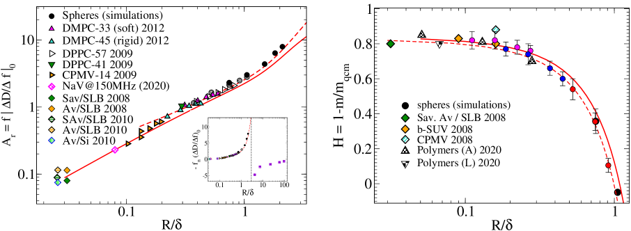
Figure 3: (a) Non-dimensional acoustic ratio $f|\Delta D/\Delta f|_{0}$ versus $R/\delta$ for experiments and simulations compared with the theoretical result obtained from Eq. 11. The solid line is the theoretical trend for $d=R$ (adsorbed particle) and the dashed line corresponds to $d=1.05R$ (small gap between the particle and surface). The acronyms used for the legend are explained in Table 1. The inset zooms out the particle size range. Beyond the divergence ($R\approx 3\delta$), the squares correspond to experimental data by Sato et al. [59] for micron-size particles. (b) Theoretical (lines) and experimental evaluation of the mass ratio $H=1-m/m_{\mathrm{QCM}}$ (see text). Filled circles correspond to simulations (color code similar to Fig. 2). The label “CPMV 2008” in (b) indicates data for the cowpea mosaic virus taken from Ref. [34], while in (a) “CPMV-14 2009” is taken from Ref. [31].

II.3 Mixtures of latex nanoparticles

The experiments by Olsson et al. [53] offers another interesting validation of the present theory. These authors considered mixtures of latex nanoparticles with nominal diameter of $24$ and $110$ nm, adsorbed on to either silica- or alumina-coated surfaces. Comparison between the purely hydrodynamic theory and the experiments will illustrate to what extent contact forces affect the acoustic response of adsorbed particles. The acoustic ratio against $\Delta f$, reported for $n=3$ of a 5 MHz AT cut, $f_{3}=15\mathrm{MHz}$ permitted us to extract values of $A_{r}$. When adding a mixture of nanoparticles, the Sauerbrey-relation 1 offers an effective particle size, but it does not provide information on the mass fraction of the different types of particles (which in the experiment were known a priori). In order to apply our theoretical result to these mixtures we need a weighted average for the impedance (note that it is incorrect to average acoustic ratios). The impedance is proportional to the wall stress which has to be summed up over the total number of particles. We denote $N_{D}$ as the number of particles with diameter $D$ (in nm). The fraction of $D=24$ particles is $\phi=N_{24}/(N_{24}+N_{110})$ and using the simple relation $m_{D}\propto N_{D}D^{3}$, we relate $\phi$ with the mass ratio $m\equiv m_{24}/m_{110}$,

$$\phi=\frac{m}{m+r^{3}},$$

where we have defined the ratio-of-diameters as $r=D_{24}/D_{110}\approx 0.218$. The weighted average for the impedance is simply,

$$Z_{\mathrm{mix}}(m)=\phi(m)Z(D_{24})+[1-\phi(m)]Z(D_{110}).$$ (12)

Theoretical curves are compared with experiments Fig. 4. The agreement is quite good and it indicates that theoretical approaches can be used to disentangle the fraction of nanoparticles size in a mixture. In mixtures with more than two components one might use the extra information from $\Delta f$ and $\Delta D$ to fit the mass fractions with the theoretical expressions. This analysis indicates that contact forces have a smaller contribution than hydrodynamics. Therefore unveiling the physical properties of contact forces, wall-induced physico-chemical interactions or any other molecular feature, first require extracting the leading effect of hydrodynamics from the analysis.

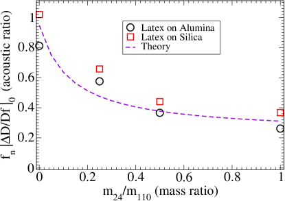
Figure 4: The acoustic ratio $A_{r}=-f(\Delta D/\Delta f)_{0}$ for mixtures of latex particles of diameter $24$ and $110\mathrm{nm}$ adsorbed on to Silica or Alumina versus the mass ratio $m\equiv m_{24}/m_{110}$. The experimental data was published in Ref. [53]. The theoretical curve is the weighted impedance (Eq. 12) $Z_{mix}=\phi Z(R_{24})+(1-\phi)Z(R_{110})$, where the particle number fraction is $\phi=m/(m+r^{3})$, with $r$ defined as the diameter-ratio, $r\equiv R_{24}/R_{110}=0.218$.

II.4 Massive particles: inertia effect

The experiments of Grunewald et al. [54] allow us to validate our theory against the effect of particle inertia. These experiments studied the acoustic response of amine functionalized porous silica nanoparticles strongly adsorbed on gold surfaces. These nanoparticles, with nominal radius $68.5\ \mathrm{nm}$, were immersed in ethanol at $T=25^{o}C$ ($\rho=0.785\ \mathrm{g/cm^{3}}$), and were prepared to present a repulsive electrostatic interaction which induced an ordered deposition, reaching a maximum coverage of about $15\%$. Values of the frequency and dissipation shifts were obtained for a range of overtones $n\in[3,13]$. The kinetic viscosity of ethanol $\nu=1.33\times 10^{-6}\ \mathrm{m^{2}/s}$ yields a penetration length $\delta_{n}=292\,n^{-1/2}\ \mathrm{nm}$ for the $n^{th}$ overtone (the fundamental resonator frequency being $f_{1}=4.95$ MHz). Mesoporous silica nanoparticles were reported to have a void fraction of about $15\%$ which yields a density in ethanol of about $\rho_{p}\approx 1.9\ \mathrm{g/cm^{3}}$. The authors evaluated the deposited mass $m_{\mathrm{QCM}}$ using the Sauerbrey relation 1, which resulted to be significantly larger than the deposited mass $m$ evaluated from the dried sample, using SEM. Moreover, contrary to the trapped-fluid model [34, 37], the mass ratio $H=1-m/m_{\mathrm{QCM}}$ was seen to significantly vary with $n$. We start by comparing our theoretical prediction for the limiting acoustic ratio $A_{r}$, obtained from a linear extrapolation of the experimental data for $-\Delta D/\Delta f$ to $\Delta f=0$. Figure 5 shows an excellent agreement for the complete overtone range. Albeit, we noticed that the predicted $A_{r}$ obtained by inserting $\rho_{p}=1.9\mathrm{g/cm^{3}}$ in Eq. 11 slightly underestimates the experimental trend. Incidentally, we found a better agreement using $\rho_{p}=1.6\ \mathrm{g/cm^{3}}$ (see Fig .5). However, the analysis of the experimental frequency $\Delta f$ revealed an interesting surprise: $\Delta f$ increases sublinearly with the deposited mass $m$. This fact is revealed in Fig. 5(b): in terms of the scaled impedance $\mathrm{Im}[\hat{\mathcal{Z}}]\sim m^{-0.18(5)}$, which implies $\Delta f\sim m^{0.81(5)}$. Theoretical predictions for $\mathrm{Im}[\hat{\mathcal{Z}}]$ [using $\rho_{p}=1.9\ \mathrm{g/cm^{3}}$, plotted as horizontal lines in Fig. 5(b)] consistently extrapolate the experimental values to the ultra-dilute regime $m\approx 0.2\mathrm{ng/mm^{2}}$ which is close to or below the QCM’s limit of detection. In such a limit, $\Delta f$ becomes slightly larger, which explains the theoretical underestimation of $A_{r}$ in Fig. 5(a). In passing, we note that the sublinear scaling $\Delta f\sim m^{0.815}$ is most probably due to hydrodynamic interaction among silica particles, but this issue is beyond the present contribution.

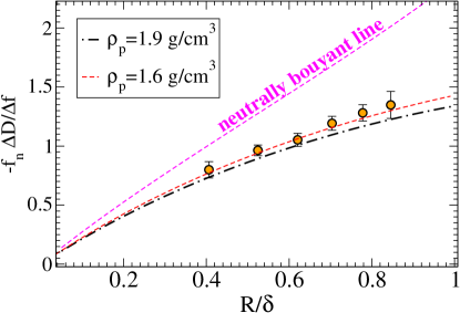
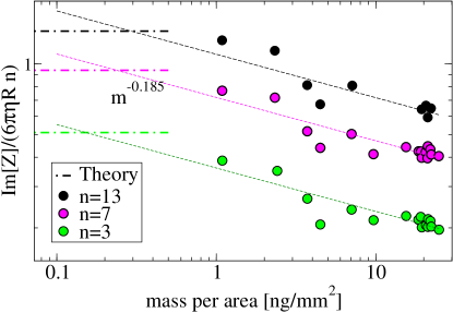
Figure 5: Comparison between the theory in Eq. 11 and experimental data reported by Grunewald et al. [54] for adsorbed Silica particles in ethanol. (a) The acoustic ratio at the low coverage limit ($\Delta f\approx 0$) and (b) the scaled impedance versus the adsorbed mass (for several overtones $n$). The horizontal dashed lines correspond to the theoretical prediction (using the experimental nanoparticle density $\rho_{p}=1.9\ \mathrm{g/cm^{3}}$), which is valid for very small coverage.

III Discussion

In summary, the present analytical study on the QCM response of discrete adsorbates shows that the main source of acoustic impedance comes from the hydrodynamic propagation of fluid-induced forces on the analyte. The sensed extra wall stress strongly depends on how mass is distributed over the resonator. And, in turn, such distribution is determined by physico-chemical forces (adhesion, dispersion and electrostatic forces, structural elasticity, etc.). This fact already permits the extraction of relevant information on the underlying microscopic configurations, uniquely invoking fluid-induced response (as done in the present work). However, physico-chemical forces are also transferred to the fluid and hydrodynamically propagate to the surface. An extension of the present theory including these secondary forces (the very purpose of QCM research), will allow deciphering and measuring subtle molecular properties, such as the different acoustic response of avidin and streptavidin, the bending rigidity and membrane fluidity of liposomes, or the reason behind the deviation from the purely hydrodynamic trend of the acoustic response of adsorbed virus capsids.

IV Methods

We have performed three-dimensional simulations of the QCM response of elastic spheres with our own software for Graphical Processors Units FLUAM [63, 64, 65] It uses the immersed boundary method (IBM) to couple the hydrodynamics of compressible flows with the dynamics of immersed molecular structures. The integration scheme is second-order accurate in space and time and the spatial discretization is based on a staggered grid [66] of cell size $h=3.958\ \mathrm{nm}$. Simulations were performed in boxes periodic in the resonator plane. Boundary conditions for the top and bottom walls were imposed using a ghost cell to easily impose a tangential velocity $v_{0}\cos(\omega t)$ (along the $x$ direction) at the bottom wall [9]. The tangential velocity gradient at the wall $(\partial v_{x}/\partial z)_{z=0}$ was calculated using a second order spatial interpolation from the upper fluid cells. The fluid traction (stress) at the resonator is measured by averaging $\eta(\partial v_{x}/\partial y)_{y=0}$ over all the surface. Using the small load approximation, the complex Fourier amplitude of the average stress directly leads to the impedance. Hollow spheres over the resonator (representing liposomes) were modelled using the elastic network model (ENM). The sphere’s surface is created by an arrangement of IBM markers in close packing, connected to their nearest neighbours (at distance $\ell\approx 2h$) by strong harmonic springs. The bending rigidity of the structure corresponds to the rigid limit ($k_{L}\ell^{2}\sim 10^{5}k_{B}T$ for $T=300\ \mathrm{K})$). The number of beads required to build the hollow sphere increases as $(R/h)^{2}$ being about $6000$ beads for a liposome of radius $R=50\,\mathrm{nm}$.

V Acknowledgments

This work was funded by the EU FET-Open Project “CATCH-U-DNA”.

VI Author contributions

R.D-B and M.M.S conceived the idea, M.M.S. derived a preliminary theoretical approach, R.D-B derived the final equations, wrote the paper and analyzed the experimental data.

VII Competing financial interests:

The authors declare no competing financial interests.

References

- [1] J Krim. Friction and energy dissipation mechanisms in adsorbed molecules and molecularly thin films. J. Adv. Phys., 61(3):155–323, 2012.
- [2] Diethlm Johannsmann. The Quartz Crystal Microbalance in Soft Matter Research, Fundamentals and modeling. Springer, 2015.
- [3] N L Bragazzi, D Amicizia, D Panatto, D Tramalloni, I Valle, and Gasparini. Quartz crystal microbalance (QCM) for public health: an overview of its applications. In Adv. Protein Chem. Struct. Biol., 101:149–211, 2015.
- [4] M Rodahl, F Hook, C Fredriksson, C A Keller, A Krozer, P Brzezinski, M Voinova, and B Kasemo. Simultaneous frequency and dissipation factor QCM measurements of biomolecular adsorption and cell adhesion. Faraday Discussions, 107:229–246, 1997.
- [5] Lia Beraldo da Silveira Balestrin, Renata Dias Francisco, Celso Aparecido Bertran, Mateus Borba Cardoso, and Watson Loh. Direct Assessment of Inhibitor and Solvent Effects on the Deposition Mechanism of Asphaltenes in a Brazilian Crude Oil. Energy & Fuels, 33:4748, 2019.
- [6] Tao Liu, Ji’an Tang, and and Long Jiang. The enhancement effect of gold nanoparticles as a surface modifier on DNA sensor sensitivity. Biochemical and Biophysical Research Communications, 313:3–7, 2004.
- [7] L B Nie, Y Yang, S Li, and N Y He. Enhanced DNA detection based on the amplification of gold nanoparticles using quartz crystal microbalance. Nanotechnology, 18:305501, 2007.
- [8] Dimitra Milioni, Pablo Mateos-Gil, George Papadakis, Achilleas Tsortos, Olga Sarlidou, and Electra Gizeli. An acoustic methodology for selecting highly dissipative probes for ultra-sensitive DNA detection. Analytical Chemistry, 92(12):8186–8193, 2020.
- [9] Adolfo Vázquez-Quesada, Marc Meléndez-Schofield, Achilleas Tsortos, Pablo Mateos-Gil, Dimitra Milioni, Electra Gizeli, and Rafael Delgado-Buscalioni. Hydrodynamics of Quartz-Crystal-Microbalance DNA Sensors Based on Liposome Amplifiers. Phys. Rev. Applied, 13(6):64059, 2020.
- [10] Vida Krikstolaityte, Jildiz Hamit-Eminovski, Laura Abariute, Gediminas Niaura, Rolandas Meskys, Thomas Arnebrant, Grzegorz Lisak, and Tautgirdas Ruzgas. Impact of molecular linker size on physicochemical properties of assembled gold nanoparticle mono-/multi-layers and their applicability for functional binding of biomolecules. Journal of Colloid and Interface Science, 543:307–316, 2019.
- [11] N.-J. Cho, K H Cheong, C Lee, C W Frank, and J S Glenn. Binding Dynamics of Hepatitis C Virus’ NS5A Amphipathic Peptide to Cell and Model Membranes. Journal of Virology, 81:6682–6689, 2007.
- [12] Ronen Fogel, Janice Limson, and Ashwin A Seshia. Acoustic biosensors. Essays in Biochemistry, 60:101–110, 2016.
- [13] Hui Yu, Xiaonan Shan, Shaopeng Wang, Hongyuan Chen, and Nongjian Tao. Plasmonic Imaging and Detection of Single DNA Molecules. ACS Nano, 8:3427–3433, 2014.
- [14] Rebecca van der Westen, Prashant K Sharma, Hans De Raedt, Ijsbrand Vermue, Henny C van der Mei, and Henk J Busscher. Elastic and viscous bond components in the adhesion of colloidal particles and fibrillated streptococci to QCM-D crystal surfaces with different hydrophobicities using Kelvin–Voigt and Maxwell models. Phys. Chem. Chem. Phys., 19(37):25391–25400, 2017.
- [15] A L Olsson, H C van der Mei, D Johannsmann, H J Busscher Busscher, and P K Sharma. Probing colloid-substratum contact stiffness by acoustic sensing in a liquid phase. Anal Chem, 84(10):4504–4512, 2012.
- [16] Ogi Hirotsugu. Wireless-electrodeless quartz-crystal-microbalance biosensors for studying interactions among biomolecules: a review. Proc. Jpn. Acad., Ser. B, 89:401–417, 2013.
- [17] G Sauerbrey. Use of quartz vibrator for weighting thin films on a microbalance. Zeitschrift fur Physik, 155:206–212, 1959.
- [18] K Keiji Kanazawa and Joseph G Gordon. Frequency of a quartz microbalance in contact with liquid. Analytical Chemistry, 57(8):1770–1771, 1985.
- [19] A J Ricco and S Martin. Acoustic wave viscosity sensor. J. Appl. Phys. Lett., 50 (21):1474–1476, 1987.
- [20] D Johannsmann, K Mathauer, G Wegner, and W Knoll. Viscoelastic Properties of Thin Films Probed With a Quartz-Crystal Resonator. Phys. Rev. B, 46 (12):7808–7815, 1992.
- [21] M V Voinova, M Rodahl, M Jonson, and B Kasemo. Viscoelastic Acoustic Response of Layered Polymer Films at Fluid-Solid Interfaces: Continuum Mechanics Approach. Phys. Scripta, 59:391–396, 1999.
- [22] Pablo Mateos-Gil, Achilleas Tsortos, Marisela Vélez, and Electra Gizeli. Monitoring structural changes in intrinsically disordered proteins using QCM-D: application to the bacterial cell division protein ZipA. Chemical Communications, 52(39):6541–6544, 2016.
- [23] Dimitra Milioni, Achilleas Tsortos, Marisela Velez, and Electra Gizeli. Extracting the Shape and Size of Biomolecules Attached to a Surface as Suspended Discrete Nanoparticles. Analytical Chemistry, 89(7):4198–4203, 2017.
- [24] Achilleas Tsortos, George Papadakis, Konstantinos Mitsakakis, Kathryn A Melzak, and Electra Gizeli. Quantitative determination of size and shape of surface-bound DNA using an acoustic wave sensor. Biophysical journal, 94(7):2706–2715, 2008.
- [25] F Mazur, M Bally, B Stadler, and R Chandrawati. Liposomes and lipid bilayers in biosensors. Adv Colloid Interface Sci., 249:88–99, 2017.
- [26] Petteri Parkkila, Mohamed Elderdfi, Alex Bunker, and Tapani Viitala. Biophysical Characterization of Supported Lipid Bilayers Using Parallel Dual-Wavelength Surface Plasmon Resonance and Quartz Crystal Microbalance Measurements. Langmuir, 34(27):8081–8091, 2018.
- [27] Ralf P. Richter and Alain R. Brisson. Following the formation of supported lipid bilayers on Mica: A study combining AFM, QCM-D, and ellipsometry. Biophysical Journal, 88:3422–3433, 2005.
- [28] Kenneth A. Marx. Quartz crystal microbalance: A useful tool for studying thin polymer films and complex biomolecular systems at the Solution-Surface interface. Biomacromolecules, 4:1099–1120, 2003.
- [29] C A Keller and B Kasemo. Surface Specific Kinetics of Lipid Vesicle Adsorption Measured With a Quartz Crystal Microbalance. B. Biophys. J., 75, (3):1397—-1402., 1998.
- [30] Diethelm Johannsmann Ilya Reviakine Marta Gallego and Edurne Tellechea. Adsorbed liposome deformation studied with quartz crystal microbalance. J. Chem. Phys., 136:84702, 2012.
- [31] Edurne Tellechea, Diethelm Johannsmann, Nicole F Steinmetz, Ralf P Richter, and Ilya Reviakine. Model-independent analysis of QCM data on colloidal particle adsorption. Langmuir, 25(9):5177–5184, 2009.
- [32] A Pomorska, D Shchukin, R Hammond, M A Cooper, G Grundmeier, and D Johannsmann. Positive frequency shifts observed upon adsorbing micron-sized solid objects to a quartz crystal mic. Anal. Chem., 82(6):2238–2245, 2010.
- [33] Susan J. Braunhut, Donna McIntosh, Ekaterina Vorotnikova, Tiean Zhou, and Kenneth A. Marx. Detection of apoptosis and drug resistance of human breast cancer cells to taxane treatments using quartz crystal microbalance biosensor technology. Assay and Drug Development Technologies, 2005.
- [34] P Bingen, G Wang, N F Steinmetz, M Rodahl, and R P Richter. Solvation effects in the quartz crystal microbalance with dissipation monitoring response to biomolecular adsorption. A phenomenological approach. Anal. Chem., 80:8880, 2008.
- [35] Christian Grunewald. Untersuchung der Adsorption und Anordnung von funktionalisierten Silica-Nanopartikeln auf Oberflächen durch die Kombination von QCM_D und REM. PhD thesis, 2015.
- [36] D Johannsmann, I Reviakine, E Rojas, and M Gallego. Effect of sample heterogeneity on the interpretation of QCM(-D) data: comparison of combined quartz crystal microbalance/atomic force microscopy measurements with finite element method modeling. Anal. Chem., 80:8891, 2008.
- [37] Zbigniew Adamczyk and Marta Sadowska. Hydrodynamic Solvent Coupling Effects in Quartz Crystal Microbalance Measurements of Nanoparticle Deposition Kinetics. Analytical Chemistry, 92(5):3896–3903, 2020.
- [38] Marc Meléndez-Schofield, Adolfo Vázquez-Quesada, and Rafael Delgado-Buscalioni. Load impedance of immersed layers on the quartz crystal microbalance: a comparison with colloidal suspensions of spheres. Langmuir, 36(31):9225–9234, 2020.
- [39] G L Dybwad. A sensitive new method for the determination of adhesive bonding between a particle and a substrate. J Appl Phys, 58(19):2789, 1985.
- [40] Adam L.J. Olsson, Henny C. van der Mei, Henk J. Busscher, and Prashant K. Sharma. Acoustic sensing of the bacterium-substratum interface using QCM-D and the influence of extracellular polymeric substances. Journal of Colloid and Interface Science, 357:135, 2011.
- [41] A Tarnapolsky and V Freger. Modeling QCM-D response to deposition and attachment of microparticles and living cells. Anal. Chem., 90:13960, 2018.
- [42] Ilya Reviakine, Diethelm Johannsmann, and Ralf P Richter. Hearing what you cannot see and visualizing what you hear: interpreting quartz crystal microbalance data from solvated interfaces. Anal. Chem., 83(23):8838–8848, 2011.
- [43] D Johannsmann and G Brenner. Frequency shifts of a quartz crystal microbalance calculated with the frequency-domain lattice–Boltzmann. Analytical Chemistry, 87(14):7476–7484, 2015.
- [44] Jurriaan J J Gillissen, Joshua A Jackman, Seyed R Tabaei, and Nam-Joon Cho. A Numerical Study on the Effect of Particle Surface Coverage on the Quartz Crystal Microbalance Response. Analytical Chemistry, 90(3):2238–2245, 2018.
- [45] J J J Gillissen, J A Jackman, S R Tabaei, B K Yoon, and N.-J. Cho. Quartz crystal microbalance model for quantitatively probing the deformation of adsorbed particles at low surface coverage. Anal. Chem., 89:11711, 2017.
- [46] S Kim and S J Karrila. Microhydrodynamics: principles and selected applications. Courier Corporation, 2013.
- [47] C. Pozrikidis. Fluid dynamics: Theory, computation, and numerical simulation, third edition. Oxgord University Press, 2016.
- [48] B. U. Felderhof. Hydrodynamic force on a particle oscillating in a viscous fluid near a wall with dynamic partial-slip boundary condition. Physical Review E, 85:046303, 2012.
- [49] A Simha, J Mo, and P J Morrison. Unsteady stokes flow near boundaries: the point-particle approximation and the method of reflections. J. Fluid Mach., 841:883–924, 2018.
- [50] B. U. Felderhof. Effect of the wall on the velocity autocorrelation function and long-time tail of Brownian motion. Journal of Physical Chemistry B, 109:21406, 2005.
- [51] P Mazur, D Bedeaux, and P Mazur. A generalization of Faxén’s theorem to nonsteady motion of a sphere through a compressible fluid in arbitrary flow. Physica, 76(3):505–515, 1974.
- [52] Elmar Bonaccurso, Michael Kappl, and Hans-Jürgen Butt. Hydrodynamic force measurements: Boundary slip of water on hydrophilic surfaces and electrokinetic effects. Phys. Rev. Lett., 88:076103, Feb 2002.
- [53] A L J Olsson, I R Quevedo, D He, M Basnet, and N Tufenkji. Using the quartz crystal microbalance with dissipation monitoring to evaluate the size of nanoparticles deposited on surfaces. ACS Nano, 7:7833, 2013.
- [54] Christian Grunewald, Madlen Schmudde, Christelle Njiki Noufele, Christina Graf, and Thomas Risse. Ordered Structures of Functionalized Silica Nanoparticles on Gold Surfaces: Correlation of Quartz Crystal Microbalance with Structural Characterization. Analytical Chemistry, 87(20):10642–10649, 2015.
- [55] Patricia M. Wolny, Joachim P. Spatz, and Ralf P. Richter. On the adsorption behavior of biotin-binding proteins on gold and silica. Langmuir, 26(2):1029–1034, 2010.
- [56] AWSensors. CATCH-U-DNA FET Open Project internal report, 2019.
- [57] J J J Gillissen, S R Tabaei, J A Jackman, and N.-J. Cho. A model derived from hydrodynamic simulations for extracting the size of spherical particles from the quartz crystal microbalance. Analyst, 142:3370, 2017.
- [58] Michael Urbakh and Leonid Daikhin. Roughness effect on the frequency of a quartz-crystal resonator in contact with a liquid. Phys. Rev. B, 49(7):4866–4870, 1994.
- [59] Aaron Webster, Frank Vollmer, and Yuki Sato. Nature Communications. Probing biomechanical properties with a centrifugal force quartz crystal microbalance, 5:5284, 2014.
- [60] G. De Fabritiis, R. Delgado-Buscalioni, and P.V. Coveney. Multiscale modeling of liquids with molecular specificity. Physical Review Letters, 97(13):134501, 2006.
- [61] R. Delgado-Buscalioni and G. De Fabritiis. Embedding molecular dynamics within fluctuating hydrodynamics in multiscale simulations of liquids. Physical Review E, 76(3), 2007.
- [62] Souhir Boujday, Aurore Bantegnie, Elisabeth Briand, Pierre Guy Marnet, Michèle Salmain, and Claire Marie Pradier. In-depth investigation of protein adsorption on gold surfaces: Correlating the structure and density to the efficiency of the sensing layer. Journal of Physical Chemistry B, 112:6708–6715, 2008.
- [63] F Balboa-Usabiaga. Fluam,https://github.com/fbusabiaga/fluam.
- [64] Florencio Balboa Usabiaga, Rafael Delgado-Buscalioni, Boyce E Griffith, and Aleksandar Donev. Inertial coupling method for particles in an incompressible fluctuating fluid. Computer Methods in Applied Mechanics and Engineering, 269:139–172, 2014.
- [65] F.B. Usabiaga, I. Pagonabarraga, and R. Delgado-Buscalioni. Inertial coupling for point particle fluctuating hydrodynamics. Journal of Computational Physics, 235:701–722, 2013.
- [66] Florencio Balboa, John B Bell, Rafael Delgado-Buscalioni, Aleksandar Donev, Thomas G Fai, Boyce E Griffith, and Charles S Peskin. Staggered schemes for fluctuating hydrodynamics. Multiscale Modeling & Simulation, 10(4):1369–1408, 2012.
- [67] F Balboa Usabiaga and R. Delgado-Buscalioni. Minimal model for acoustic forces on Brownian particles. Physical Review E, 88(6):63304, 2013.
- [68] S. Delong, F.B. Usabiaga, R. Delgado-Buscalioni, B.E. Griffith, and A. Donev. Brownian dynamics without Green’s functions. Journal of Chemical Physics, 140(13), 2014.
- [69] Paul J Atzberger. Stochastic Eulerian Lagrangian methods for fluid–structure interactions with thermal fluctuations. Journal of Computational Physics, 230(8):2821–2837, 2011.