First-passage times to quantify and compare structural correlations and heterogeneity in complex systems

Abstract

Virtually all the emergent properties of a complex system are rooted in the non-homogeneous nature of the behaviours of its elements and of the interactions among them. However, the fact that heterogeneity and correlations can appear simultaneously at local, mesoscopic, and global scales, is a concrete challenge for any systematic approach to quantify them in systems of different types. We develop here a scalable and non-parametric framework to characterise the presence of heterogeneity and correlations in a complex system, based on the statistics of random walks over the underlying network of interactions among its units. In particular, we focus on normalised mean first passage times between meaningful pre-assigned classes of nodes, and we showcase a variety of their potential applications. We found that the proposed framework is able to characterise polarisation in voting systems, including the UK Brexit referendum and the roll-call votes in the US Congress. Moreover, the distributions of class mean first passage times can help identifying the key players responsible for the spread of a disease in a social system, and comparing the spatial segregation of US cities, revealing the central role of urban mobility in shaping the incidence of socio-economic inequalities.

The elements of a variety of complex systems can be naturally associated to one of a small number of classes or categories. Typical examples include the organisation to which an individual belongs [1], the political party of a voter [2], the income level of a household [3], or the functional group of a neuron [4]. Quite often, the co-existence of nodes belonging to different classes and the interactions among those classes play a fundamental role in the functioning of a system. For instance, economic and ethnic segregation in cities is known to be associated to the emergence of social inequalities [5, 6]. Similarly, the organisation of neural cells in the brain and the intricate patterns of relations among different functional areas are known to be responsible for the large variety of cognitive tasks that we as humans are able to perform [7, 8]. However, obtaining a robust and non-parametric quantification of the heterogeneity of class distributions, especially in systems consisting of a large number of interconnected discrete components, is still an outstanding problem.

We propose here a principled methodology to quantify the presence of correlations and heterogeneity in the distribution of classes or categories in a complex system. The method is based on the statistics of passage times of a uniform random walk on the graph of interconnections among the units of the system. For instance, in the case of a social system we can construct a graph among individuals based on the observed relations or contacts among them. Similarly, in a urban system we can consider the network of adjacency between census tracts or the connections among census tracts due to human mobility flows. The method we propose moves from the classical research on mean first passage times between pairs of nodes in a graph [9, 10, 11, 12], and focuses instead on the distribution of Class Mean First Passage Times (CMFPT) i.e., the expected number of steps needed to a random walker to visit for the first time a node of a certain class $\beta$ when it starts from a node of class $\alpha$. By normalising class mean first passage times with respect to a null-model where classes are reassigned to nodes uniformly at random, we can effectively quantify and compare the heterogeneity of class distributions in systems of different nature, size, and shape.

We first test the framework on a variety of systems with simple geometries and ad-hoc class assignments, and then we use it in three real-world scenarios, namely the quantification of polarisation in the Brexit referendum and in the US Congress since 1926, the role of face-to-face interactions among individuals in the spread of an epidemics, and the relation between economic segregation and prevalence of crime in the 53 US cities with more than one million citizens.

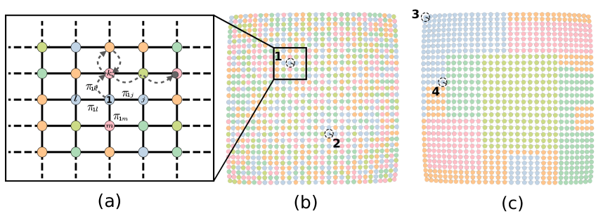
Figure 1: The statistics of the amount of time needed to a random walker to hit a node of a given class when starting from another node of the graph encodes useful information about the presence of heterogeneity and correlations in the distributions of node classes. In panel (a) we show a sketch of the trajectory of a random walker over the grid. In panel (b) the nodes of a square lattice are assigned to one of five available classes uniformly at random. As a consequence, the time needed to a random walker to hit an orange node when starting by node $1$ is comparable to the time needed when starting from node $2$. In panel (c) the assignment of nodes to classes creates homogeneous clusters of nodes of the same colour. As a consequence, the time needed to a random walker to hit an orange node when starting from node $3$ is much higher than the time needed when starting from node $4$.

I Model

Let us consider a graph $G(V,E)$ with $|V|=K$ edges on $|V|=N$ nodes with adjacency matrix $A=\{a_{ij}\}$, and a given colouring function $f:V\rightarrow\mathcal{C},\quad\mathcal{C}=\{1,2,\ldots,C\}$, that associates each node $i$ of $G$ to a discrete label $f(i)=c_{i}$. Let us also consider a random walk on $G$, defined by the transition matrix $\Pi=\{\pi_{ij}\}$ where $\pi_{ij}$ is the probability that a walker at node $i$ jumps from node $i$ to node $j$ in one step (see Fig. 1(a)). In general, $\Pi$ could be any row-stochastic transition matrix, but in the following we will consider only uniform random walks. We are interested here in the statistical properties of the symbolic dynamics $W_{i}=\{c_{i0},c_{i1},\ldots\}$ of node labels or classes visited by the walk $W$ when starting from $i$. This dynamics obviously contains information about the existence of correlations and heterogeneity in the distribution of colours.

In the regular square lattice shown in Fig. 1(b), for example, a function $f$ associates 5 distinct colours to nodes of the graph uniformly at random, while in Fig. 1(c), instead, the colouring function induces a small number of homogeneous clusters. We expect that, for long-enough times, all the trajectories of random walks starting from each of the $N$ nodes of the graph in panel (b) will be associated with the same symbolic dynamics, thus becoming indistinguishable. Indeed, that system has neither structural heterogeneity, since all the nodes have the same degree (except for the nodes at the border of the grid), nor inhomogeneity in class assignments, since the probability for a node to belong to a certain class does not depend on its position in the graph or on the classes of its neighbours. In particular, a random walker starting at any node belonging to, say, the light-blue class (see nodes $1$ and $2$ in panel (b)) will require on average a small number of steps to hit a node in the orange cluster, since orange nodes can be found in the vicinity of any blue node.

If the colouring function induces compact clusters of nodes belonging to the same class, as in the lattice shown in Fig. 1(c), then the statistical properties of the symbolic dynamics $W_{i}$ will heavily depend on the starting node $i$, despite the fact that almost all the nodes have identical degree. In particular, a random walker starting in the blue cluster at the top-left corner of the graph (node $3$) will in general require a very large number of steps before hitting for the first time an orange node. Conversely, a random walker starting at node $4$ will hit a node in the orange cluster in a much smaller number of steps, just because one of its immediate neighbours is indeed orange.

I.1 Class Mean First Passage Time

A quantity of interest in the study of a symbolic dynamics over graphs is the expected time needed to hit a node of a given colour $\alpha$ for the first time, usually know in the literature as the hitting time or mean first passage time (MFPT) to class $\alpha$ [13]. We denote as $T_{i,\alpha}$ the average mean first passage time from node $i$ to any node of class $\alpha$, i.e., the expected number of steps needed to a walk starting on $i$ to visit for the first time any node $j$ such that $f(j)=\alpha$. Following the formalism to derive the mean first passage times between nodes in a graph, we can write a set of self-consistent equations for $T_{i,\alpha}$ [14]:

$$T_{i,\alpha}=1+\sum_{j=1}^{N}\left(1-\delta_{f(j),\alpha}\right)\pi_{ij}T_{j,\alpha}.$$ (1)

We can derive an analytic solution for Eq. (1) which depends only on the structure of the graph and on the colouring function $f$. Let us denote as $T_{\alpha}$ the column vector of hitting times from nodes of class $\beta\neq\alpha$ to nodes of class $\alpha$. By convention we set $\{T_{\alpha}\}_{i}=0$ if $f(i)=\alpha$. The self-consistent equation for hitting times can be written as:

$$T_{\alpha}=D_{\overline{\alpha}}+\Pi_{\overline{\alpha}}T_{\alpha}$$

where $\Pi_{\overline{\alpha}}$ is the transition matrix of the walk where all the rows and columns corresponding to nodes of class $\alpha$ are set to zero. We denote by $D_{\alpha}$ the indicator vector of nodes belonging to class $\alpha$, and by $D_{\overline{\alpha}}=\bm{1}_{N}-D_{\alpha}$ the indicator vector of nodes not belonging to class $\alpha$, i.e., $\{D_{\overline{\alpha}}\}_{i}=1-\delta_{f(i),\alpha}$. This leads to the solution:

$$T_{\alpha}=\left[I-\Pi_{\overline{\alpha}}\right]^{-1}D_{\overline{\alpha}}$$ (2)

The average Class MFPT $\tau_{\alpha\beta}$ from class $\alpha$ to class $\beta$ is computed as:

$$\tau_{\alpha\beta}=\frac{1}{N_{\alpha}}\sum_{j=1}^{N}D_{\alpha}^{\intercal}T_{\beta}$$ (3)

where $N_{\alpha}$ is the number of nodes belonging to class $\beta$.

The return time to class $\alpha$, that is the expected number of steps needed to a walker starting on a node of class $\alpha$ to hit a node of class $\alpha$ (including its starting point) can be computed in a similar way. The forward equation for the hitting time to class $\alpha$ from a node of class $\alpha$ reads:

$$R_{i,\alpha}=\sum_{j=1}^{N}\delta_{f(j),\alpha}\pi_{ij}+\sum_{j=1}^{N}(1-\delta_{f(j),\alpha})\pi_{ij}(1+T_{j,\alpha})$$ (4)

where the first contribution accounts for the neighbours of node $i$ which actually belong to class $\alpha$, while the second contribution corresponds to walks passing through immediate neighbours of $i$ not belonging to class $\alpha$. The equation can be written in a compact form as:

$$R_{\alpha}=\Pi_{\alpha\alpha}D_{\alpha}+\Pi_{\alpha\overline{\alpha}}\left[T_{\alpha}+D_{\overline{\alpha}}\right]$$ (5)

where $R_{\alpha}$ is the vector of return times to class $\alpha$, such that $\left\{R_{\alpha}\right\}_{i}=0$ if $f(i)\neq\alpha$, and $T_{\alpha}$ is the vector of MFPT to class $\alpha$ from nodes that do not belong to class $\alpha$, as above. Here we denote by $\Pi_{\alpha\alpha}$ is the transition matrix of the walk restricted to nodes of class $\alpha$, i.e., whose generic element $\pi_{ij}$ is set to $0$ if either $i$ or $j$ do not belong to class $\alpha$. Similarly, $\Pi_{\alpha\overline{\alpha}}$ is the transition matrix restricted to links from nodes of class $\alpha$ to nodes not in class $\alpha$. By solving Eq. (2) and Eq. (5) for the grid lattice shown in Fig. 1(b) we obtain the distribution of CMFPTs:

$\tau_{\alpha\beta}$	${\color[rgb]{0.757,0.831,0.902}\bullet}$	${\color[rgb]{0.8,0.859,0.525}\bullet}$	${\color[rgb]{1,0.77,0.549}\bullet}$	${\color[rgb]{1,0.741,0.776}\bullet}$	${\color[rgb]{0.678,0.859,0.718}\bullet}$
${\color[rgb]{0.757,0.831,0.902}\bullet}$	5.14	8.60	8.03	8.20	7.02
${\color[rgb]{0.8,0.859,0.525}\bullet}$	7.91	5.58	7.82	7.96	7.18
${\color[rgb]{1,0.77,0.549}\bullet}$	7.62	8.24	4.89	8.68	7.20
${\color[rgb]{1,0.741,0.776}\bullet}$	7.82	8.20	8.87	4.77	7.12
${\color[rgb]{0.678,0.859,0.718}\bullet}$	7.36	8.46	7.94	8.05	4.69

while for the lattice with clusters in Fig. 1(c) we get:

$\tau_{\alpha\beta}$	${\color[rgb]{0.757,0.831,0.902}\bullet}$	${\color[rgb]{0.8,0.859,0.525}\bullet}$	${\color[rgb]{1,0.77,0.549}\bullet}$	${\color[rgb]{1,0.741,0.776}\bullet}$	${\color[rgb]{0.678,0.859,0.718}\bullet}$
${\color[rgb]{0.757,0.831,0.902}\bullet}$	5.1	255.5	183.8	263.7	158.6
${\color[rgb]{0.8,0.859,0.525}\bullet}$	271.2	4.8	127.6	222.3	116.8
${\color[rgb]{1,0.77,0.549}\bullet}$	255.4	201.5	5.0	150.6	179.3
${\color[rgb]{1,0.741,0.776}\bullet}$	302.4	200.4	51.4	4.9	211.3
${\color[rgb]{0.678,0.859,0.718}\bullet}$	293.1	142.1	83.5	326.2	4.9

Notice that, as expected, the CMFPTs in the lattice with compact clusters are in general much higher than those observed in the same lattice with uniformly random class assignments. Moreover, both cases we have in general $\tau_{\alpha\beta}\neq\tau_{\beta\alpha}$, since CMFPTs depend primarily on the shape and size of clusters and on the actual fine-grain arrangement of colours.

I.2 Mean-Field approximation

The expressions for class mean first passage time and class return time provided in Eq. (2) and Eq. (5) are exact, but they have the drawback of being computationally intensive for graphs with a large number of nodes. It is possible to construct C-class mean-field approximations of these expressions, by representing the behaviour of all the nodes of a class with a single node, and looking at the graph of node classes. If we denote by $\pi_{\alpha\beta}$ the probability for a walker to jump in one step from any node of class $\alpha$ to any node of class $\beta$, e.g. expressed as the total fraction of edges from nodes of class $\alpha$ to nodes of class $\beta$, the general Mean-Field equation for CMFPT reads:

$$T_{\beta\alpha}^{\rm MF}=D_{\overline{\alpha}}+\sum_{\gamma\neq\alpha}\pi_{\beta\gamma}T_{\gamma\alpha}$$

which can be written in compact form as:

$$T_{\alpha}^{\rm MF}=D_{\overline{\alpha}}+\Pi_{\overline{\alpha}}T_{\alpha}^{\rm MF}$$

where by definition $\{T_{\alpha}^{\rm MF}\}_{\alpha}=0$ and $\Pi_{\overline{\alpha}}$ is the transition matrix where the row and column corresponding to class $\alpha$ are set equal to zero as above. The solution to this equation is:

$$T_{\alpha}^{\rm MF}=\left[I-\Pi_{\overline{\alpha}}\right]^{-1}D_{\overline{\alpha}}$$

Notice that this equation is formally identical to Eq. (2), with the only difference that it deals with mean first passage times from all other classes to class $\alpha$, while Eq. (2) provides the mean first passage times from all the nodes in other classes to class $\alpha$. However, the mean-field approximation only retains information about the average probability of jumping between two classes in one time-step, which indeed discards all the (possibly relevant) structural information contained in the underlying graph. For instance, if we use the mean-field approximation for the lattice with random colour assignments shown in Fig. 1(b), we get the solutions:

$\tau_{\alpha\beta}$	${\color[rgb]{0.757,0.831,0.902}\bullet}$	${\color[rgb]{0.8,0.859,0.525}\bullet}$	${\color[rgb]{1,0.77,0.549}\bullet}$	${\color[rgb]{1,0.741,0.776}\bullet}$	${\color[rgb]{0.678,0.859,0.718}\bullet}$
${\color[rgb]{0.757,0.831,0.902}\bullet}$	5.05	5.09	4.98	5.10	5.08
${\color[rgb]{0.8,0.859,0.525}\bullet}$	5.48	5.36	5.40	5.46	5.48
${\color[rgb]{1,0.77,0.549}\bullet}$	4.78	4.80	4.90	4.98	4.94
${\color[rgb]{1,0.741,0.776}\bullet}$	4.92	4.89	5.00	4.94	4.90
${\color[rgb]{0.678,0.859,0.718}\bullet}$	4.74	4.74	4.80	4.74	4.80

where the values of CMFPT between different classes are substantially different from those computed above using Eq. (2).

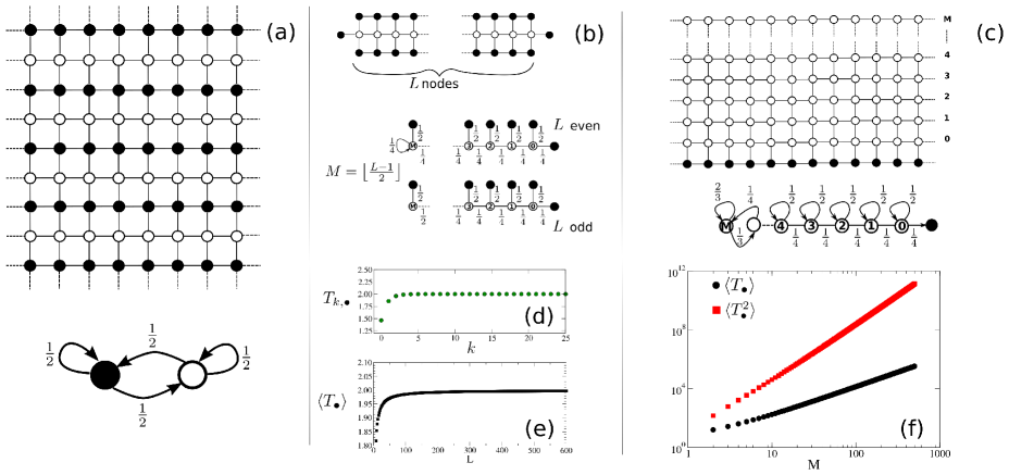
Figure 2: (a)-(c): Three simple 2-colour geometries on infinite 2D lattices (top), and the equivalent minimal graphs used to compute inter-class mean first passage times (bottom). When nodes are organised in rows of alternate colours (a) the equivalent graph contains only two nodes with symmetric connections. The equivalent graph of a chain of $\circ$ nodes surrounded by $\bullet$ nodes (b) is equivalent to a comb graph, while an infinite cylinder of with $M+1$ rows of $\circ$ nodes (c) reduces to the chain with $M+1$ $\circ$ nodes. In the case of the chain graph in (b), the CMFPT of a node as a function of its distance $k$ from the endpoint converges to $2$ as $k$ increases (d). Similarly, the average CMFPT to $\bullet$ converges to $2$ when the length $L$ of the chain increases (e). In panel (f) we show the first two moments of $T_{k,\bullet}$ in an infinite cylinder, as a function of the height of the cylinder.

I.3 Normalisation of CMFPT distributions

As we will see in the following sections, the statistics of CMFPT depend substantially on the shape, size, and organisation of class assignments. To allow a fair comparison of CMFPT in systems with different sizes and shapes, we compute the normalised inter-Class Mean First Passage Time $\widetilde{\tau}_{\alpha\beta}=\tau_{\alpha\beta}/\tau^{\rm null}_{\alpha\beta}$. This quantity is the ratio between the expected number of time steps needed to a walk that starts on a node of class $\alpha$ to reach a node of class $\beta$ for the first time, and the corresponding value in a null-model where classes are assigned to nodes uniformly at random, by preserving their relative abundance. Notice that if classes are distributed uniformly across the system, then $\widetilde{\tau}_{\alpha\beta}\approx 1,\>\forall\alpha,\beta$, while in the presence of spatial correlations $\widetilde{\tau}_{\alpha\beta}$ will deviate from 1. By using $\widetilde{\tau}_{\alpha\beta}$ we properly take into account several common confounding factors, including an uneven abundance of colours, differences in size and shape, and the effect of borders, thus making it possible to compare different systems on common grounds. Depending on the size of the system, the computation of $\tau_{\alpha\beta}^{\rm null}$ is based on the average over $10^{3}-10^{5}$ independent assignments of classes to the nodes of the original graph.

I.4 Computation of CMFPT distributions in real-world networks

In the following we will compute and use the distribution of CMFPT in a variety of synthetic and real-world networks. If a system is naturally represented by an unweighted network, the elements of the transition matrix of the random walker will be set to $\pi_{ij}=\frac{a_{ij}}{k_{i}}$, where $a_{ij}=1$ is there is an edge from node $i$ to node $j$, and $k_{i}=\sum_{j}a_{ij}$ is the (out-) degree of node $i$. If the network is weighted, instead, the elements of the transition matrix will be $\pi_{ij}=\frac{w_{ij}}{s_{i}}$, where $w_{ij}$ is the weight of the edge connecting node $i$ to node $j$, and $s_{i}=\sum_{j}w_{ij}$ is the (out-) strength of node $i$. For networks with up to $N\sim 10^{4}$ nodes, we solved Eq.(2) and Eq.( 5) exactly, using standard linear algebra packages. For larger graphs we reverted instead to Monte-Carlo simulations, where we estimated the value of $T_{i,\alpha}$ for each node $i$ of the graph as the average over $10^{4}\sim 10^{6}$ random walks originating at that node, and then obtained $\tau_{\alpha\beta}$ using Eq. (3).

II Simple geometries

We compute here the distribution of CMFPT for some simple geometries with simple class assignments. These examples aim at showing that CMFPT depends heavily on class assignment and on the way nodes belonging to the same classes are arranged. In all these cases, the symmetric nature of colour assignments will allow us to perform the computations on a minimal weighted graph whose distribution of CMFPT is identical to that of the original system. Notice that those minimal weighted graphs provide exact solutions for the original colour assignment they represent, and should not be confused with mean-field approximations.

The first example is that of a 2-dimensional square lattice with periodic boundary conditions (a torus), whose nodes are organised in alternate stripes of black and white nodes, as shown in Fig. 2(a). Thanks to the symmetric nature of this specific colour assignment, a uniform random walk on that graph is effectively equivalent to a random walk on the weighted minimal two-node graph shown in the lower panel of Fig. 2(a), with the transition matrix:

$$\Pi=\begin{bmatrix}\frac{1}{2}&\frac{1}{2}\\ \frac{1}{2}&\frac{1}{2}\\ \end{bmatrix}$$

The hitting time to the black node in the minimal equivalent graph when starting from the white node can be written as:

$$T_{\circ,\bullet}=1+\frac{1}{2}T_{\circ,\bullet}$$

which gives $T_{\circ,\bullet}=2$ and, by symmetry, also $T_{\bullet,\circ}=2$.

As a second example we consider a finite chain of white nodes surrounded by black nodes, as shown in the top panel of Fig 2(b). We are interested here in showing how the length $L$ of a linear cluster of a given colour influences the distribution of CMFPT across the cluster, so we will focus on the CMFPT from nodes of class $\circ$ to nodes of class $\bullet$. In this case the system has a mirror symmetry, which effectively allows us to focus on the $\left\lceil\frac{L}{2}\right\rceil$ on either side of the chain. The only caveat is that weighted minimal graphs associated to chains with even length $L$ are slightly different from those associated to chains with odd length, as shown in Fig. 2(b). For $L\geq 6$, the closed expression for the distribution of CMFPT from each node in the chain is:

$$T_{k,\bullet}=\left[\frac{4+A_{M-1}}{4-B_{M-1}}\right]\prod_{\ell=1}^{k}B_{M-\ell}+\sum_{j=1}^{k-1}A_{M-k+j}\prod_{\ell=0}^{j-1}B_{M-k+\ell}$$ (6)

where $M=\left\lfloor\frac{L-1}{2}\right\rfloor$, and $A_{k}$ and $B_{k}$ are two rational sequences whose form depends on whether the length of the chain is even or odd. More details about the derivation are provided in Appendix A.1, where we also compute the distributions for $1\leq L<6$. In Fig. 2(d) we report the distribution of $T_{k,\bullet}$ across the chain, while in Fig. 2(e) we show the average CMFPT to nodes of class $\bullet$. Notice that when $L\gg 1$, $\langle T_{\bullet}\rangle$ converges towards $2$, which is the same value obtained in the case of a lattice with rows of alternate colours seen above, as expected.

As a final example we consider the infinite cylinder shown in the top panel of Fig. 2(c), where the nodes in the upper $M+1$ rows are of class $\circ$ and those in the bottom row are of class $\bullet$. The aim of this example is to show the behaviour of CMFPT as a cluster becomes deeper, i.e., as the nodes in the cluster of a certain class are placed farther away from the frontier with the other cluster. For our purposes, this geometry is effectively equivalent to the linear chain of nodes shown in the bottom half of Fig 2(c), where each row of the original graph is represented by a single node in the minimal graph, with an appropriately-weighted self-loop. We can write a set of self-consistent equations for the hitting time to class $\bullet$ for a walk started on each of the rows $k=0,1,\ldots,M$:

$$T_{0,\bullet}= 2+\frac{1}{2}T_{1,\bullet}$$ (7)

$$T_{k,\bullet}= 2+\frac{1}{2}\left[T_{k-1,\bullet}+T_{k+1,\bullet}\right],\>k=1,\ldots,M-1$$

$$T_{M,\bullet}= 3+T_{M-1,\bullet}$$

whose solution is:

$$T_{k,\bullet}=(k+1)(3+4M-2k),\quad k=0,1,\ldots M-1$$ (8)

and

$$T_{M,\bullet}=3+M(5+2M)$$ (9)

The full derivation is reported in Appendix A.2.

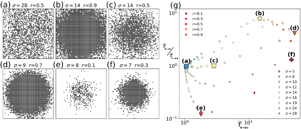
Figure 3: (a)-(f) Snapshots of the model for different values of the parameters $\sigma$ and ratio. (a) $\sigma=28$ and ratio=0.5 (b) $\sigma=14$ and ratio=0.9 (c) $\sigma=14$ and ratio=0.5 (d) $\sigma=9$ and ratio=0.7 (e) $\sigma=8$ and ratio=0.1 (f) $\sigma=7$ and ratio=0.3. (g) Transition in the coordinates $\widetilde{\tau}_{\bullet\to\circ}/\widetilde{\tau}_{\circ\to\bullet}$ as a function of $\widetilde{\tau}_{\bullet\to\circ}$ for different values of $\sigma$ and the ratio between colours. The colour of each point corresponds to the value of $\sigma$ in the Gaussian first and type of marker to the ratio between colours. Simulations were performed in a regular lattice of size $60\times 60$.

In Fig. 2(f) we show the scaling of average mean first passage time to class $\bullet$, defined as:

$$\langle T_{\bullet}\rangle =\frac{1}{M+1}\sum_{k=0}^{M}T_{k,\bullet}=\frac{8M^{3}+33M^{2}+43M+18}{6(M+1)}$$ (10)

$$\simeq\frac{1}{6}\left(8M^{2}+33M\right)$$ (11)

where the approximation is accurate for $M\gg 1$. This means that the average MFPT to class $\bullet$ scales as the square of the height of the cylinder. In the same panel we also show the scaling of the second moment of $T_{k,\bullet}$:

$$\langle T_{k,\bullet}^{2}\rangle=\frac{32M^{5}+355M^{4}}{15(M+1)}+o(M^{2})\simeq\frac{32M^{4}+355M^{3}}{15}$$ (12)

which indicates that the standard deviation of $T_{k,\bullet}$ is a function that grows as $O(M^{2})$ as well. In other words, the deeper a cluster the much higher the CMFPT to its border, and the much wider the distribution of the MFPT from any single node of the cluster to the border.

III Synthetic colourings in two-dimensional lattices

We study here the distribution of CMFPTs in a two-dimensional square lattice with $N=L\times L$ nodes. Here each node is associated to one of two possible classes, namely $\bullet$ or $\circ$, depending on their position in the lattice. Without lack of generality, we set the relative abundance of $\bullet$ nodes $r=\frac{N_{\bullet}}{N}$. Then we assign $N_{\bullet}$ nodes to class $\bullet$ sampling their coordinates $(x,y)$ from a symmetric two-dimensional Gaussian distribution centred in the middle of the lattice, with standard deviation equal to $\sigma$:

$$P(x)=\frac{1}{{\sigma\sqrt{2\pi}}}e^{{{-\left({x-L/2}\right)^{2}}\mathord{\left/{\vphantom{{-\left({x-\mu}\right)^{2}}{2\sigma^{2}}}}\right.\kern-1.2pt}{2\sigma^{2}}}},$$ (13)

By tuning $r$ and $\sigma$ this model allows for a continuous transition between homogeneous distributions of colours and patterns with strong class segregation. In Fig. 3(a)-(f) we show sample sketches of how the spatial distribution of colours looks like as a function of $\sigma$ and $r$. For very large values of $\sigma$, the picture approaches a homogeneous distribution, regardless of the relative abundance of the two colours. As $\sigma$ decreases, instead, the nodes of class $\bullet$ will become more strongly clustered around the centre. The role of the relative abundance of colours is evident from the comparison of panel (b) and panel (c), which are two configurations with the same $\sigma$ respectively for $r=0.9$ and $r=0.5$. In particular, we note that the relative abundance of the two colours also has a non-trivial role in determining the degree of mixing between the two classes, since more $\circ$ nodes can be found inside the $\bullet$ cluster for $r=0.5$ than for $r=0.9$.

A summary of the interplay between these two parameters is reported in Fig. 3(g), where we show the quantities $\widetilde{\tau}_{\bullet\to\circ}$ and $\widetilde{\tau}_{\bullet\to\circ}/\widetilde{\tau}_{\circ\to\bullet}$ for a variety of values of $r$ and $\sigma$ (the points in panel (g) corresponding to the configurations in panels (a)-(f) are labelled accordingly). For large values of $\sigma$, we expect a more homogeneous distributions of the two colours, (see Fig.3(a)), and indeed we have $\widetilde{\tau}_{\bullet\to\circ}\simeq 1$, meaning that the relative distribution of CMFPT from $\bullet$ nodes is compatible with the one observed in the corresponding null model. At the same time, the ratio $\widetilde{\tau}_{\bullet\to\circ}/\widetilde{\tau}_{\circ\to\bullet}$ is close to $1$ as well, meaning that the normalised CMFPTs of the two classes are indistinguishable. As $\sigma$ decreases, the $\bullet$ cluster becomes more prominent, but the actual relation between $\widetilde{\tau}_{\bullet\to\circ}$ and $\widetilde{\tau}_{\bullet\to\circ}/\widetilde{\tau}_{\circ\to\bullet}$ will depend on the value of $r$. In particular, if $r>0.5$, i.e., nodes of class $\bullet$ are the majority (see Fig. 3(b) and Fig. 3(d)), the ratio $\widetilde{\tau}_{\bullet\to\circ}/\widetilde{\tau}_{\circ\to\bullet}$ normally remains larger than $1$. This is again expected, since a deeper cluster of $\bullet$ nodes causes an increase in the CMFPT from $\bullet$ to $\circ$ nodes, along the same lines of the increase in CMFPT observed in the simple geometry shown in Fig. 2(c). Conversely, if $r<0.5$ then $\bullet$ nodes are interspersed within a large cluster of $\circ$ nodes (see Fig. 3(e)), making it harder for a walker started at a $\circ$ node to find a $\bullet$ node. This results in values of $\widetilde{\tau}_{\circ\to\bullet}$ larger than $1$, i.e., much longer than in the corresponding null-model, and in $\widetilde{\tau}_{\bullet\to\circ}/\widetilde{\tau}_{\circ\to\bullet}<1$. There are some particular situations (see Fig. 3(c),(f)) in which despite the increase in $\widetilde{\tau}_{\bullet\to\circ}$, the ratio $\widetilde{\tau}_{\bullet\to\circ}/\widetilde{\tau}_{\circ\to\bullet}$ remains close to $1$. This is due to the fact that in these cases the two classes are distributed in a similar fashion, and the relative depths of the two clusters are indeed comparable.

It is worth noting that the $(\widetilde{\tau}_{\bullet\to\circ},\widetilde{\tau}_{\bullet\to\circ}/\widetilde{\tau}_{\circ\to\bullet})$ phase space provides a very intuitive interpretation and a powerful visualisation of the heterogeneity of distributions of two classes, and it would thus be quite useful to characterise the spatial heterogeneity of generic binary feature distributions and point statistics [15, 16].

IV Polarisation and segregation in voting dynamics

Among the variety of social dynamics that exhibit complex behaviours, voting is possibly one of the most interesting. And not just because anything concerning politics can spur endless and ferocious discussions, but also because voting patterns are the result of the interplay of a variety of factors that are generally difficult to model in an accurate way, including socio-economic and cultural background and spatial and temporal correlations [2, 17]. We focus here on two examples where voting dynamics result in the emergence of heterogeneity and correlations, namely the spatial clustering of Leave/Remain voters in the Brexit referendum and the polarisation of opinions of roll-call votes in the US Congress.

IV.1 Spatial heterogeneity of Brexit vote

Here we show how inter-class mean first-passage times can be used to quantify the spatial segregation of voting patterns. We consider the results of the so-called “Brexit” referendum, held in the United Kingdom in 2016 to decide whether to leave the European Union. The referendum had a turnout of $72.2\%$, and $51.9\%$ of the voters expressed the preference to leave the EU. The results of the referendum have been analysed in several works [18] which have outlined interesting correlations of voting preference with a variety of socio-economic indicators, including age, income level, unemployment, and level of education [19]. One of the most intriguing aspects of the results was that the vote was highly segregated. Indeed, highly urbanised areas, as well as the majority of constituencies in Scotland, voted preferentially for Remain, while the rest of the country expressed a preference to Leave.

We constructed the planar graph of constituencies in Great Britain (i.e., all the mainland constituencies in England, Wales, and Scotland, leaving out the few constituencies in Northern Ireland), where each node is associated to a constituency and a link between two nodes exists if the corresponding constituencies border each other. We assigned each node to either Leave or Remain according to which party won the majority of votes in the corresponding constituency. We then computed the normalised average CMFPT pattern for Remain (R) and Leave (L), we obtained the values shown in Table 1(a).

$\widetilde{\tau}_{\alpha\beta}$ L R L 0.976 2.857 R 12.304 1.008	$\widetilde{\tau}_{\alpha\beta}$ L R L 1.018 1.057 R 1.090 0.981
(a)	(b)

Table 1: (a) Normalised CMFPT between constituencies which voted for Leave (L) or Remain (R) in the Brexit referendum. Note that $\widetilde{\tau}_{LR}$ is almost six times smaller than $\widetilde{\tau}_{RL}$. (b) If we consider the ensemble of colour assignments where a node is assigned to Leave (Remain) with a probability equal to the fraction of voters supporting Leave (Remain) in that constituency, the resulting normalised CMFPT is not distinguishable from the null-model distribution.

It is worth noting that while the normalised return time to each class is close to $1$ in both cases, i.e., it is consistent with the corresponding null model where classes are reassigned to nodes uniformly at random, the proper inter-class MFPTs exhibit a pronounced disparity between the two classes. In particular, the normalised CMFPT from Leave to Remain $\widetilde{\tau}_{LR}$ is much smaller (2.827) than its counterpart $\widetilde{\tau}_{RL}$ (12.304). This means that, on average, in this graph is much easier for a random walker starting at a node whose citizens expressed a majority of votes for Leave to arrive at a node where people preferentially voted for Remain, than the other way around. Or, putting it in another way, it was much easier for a Leave supporter wandering through the graph to meet a Remain supporter than the other way around.

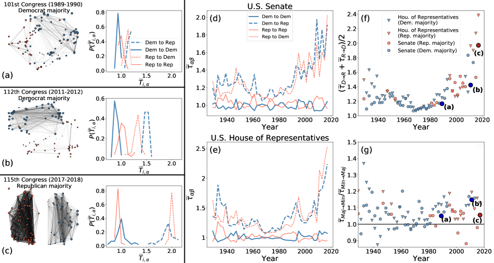
Figure 4: Roll-call polarisation in the Senate and the U.S. House of Representatives. (a)–(c) Three networks connecting the members of the senate where edge weights correspond to the number of calls in which the corresponding two members voted the same on a roll call, and the corresponding distribution of CMFPT from the nodes (members) to each of the parties. (a) 101st Congress (1989-1990), (b) 112th Congress (2011-2012) and (c) 115th Congress (2017-2018). (d)-(e) Temporal evolution of $\tau_{\alpha\beta}$ in (d) the Senate and (e) the U.S. House of Representatives. (f) Temporal evolution of polarisation in the the Senate and the U.S. House of Representatives, as measured by $(\widetilde{\tau}_{D\to R}+\widetilde{\tau}_{R\to D})/2$. (f) Temporal evolution of $\widetilde{\tau}_{Maj\to Min}/\widetilde{\tau}_{Min\to Maj}$. The fact that this quantity is larger than one in most of the terms indicates that the party with a majority is the one responsible for the largest contribution to polarisation in the corresponding term.

A possible interpretation of this result is the presence of a structural reinforcement of segregation. Indeed, if we assume that voters could influence each other by discussing the matter of the referendum with other voters holding opposite opinions, then a person determined to vote for Remain would have had a much harder time finding a Leave supporter to convince. On the contrary, Leave supporters would have been able to find Remain supporters much more easily, as Leave constituencies are on average closer (in terms of MFPT) to other Remain constituencies than the other way around.

However, this picture is completely reversed if we take into account the actual percentage of votes for Leave and Remain in each constituency, instead of noting only which party got a majority. We considered an ensemble of colour assignments obtained by assigning colour $L$ to node $i$ with probability $p_{L}(i)$ equal to the percentage of Leave voters in constituency $i$. For instance, if in a given constituency $i$ we had $45\%$ of votes for Leave, then node $i$ will be assigned to class $L$ with probability $0.45$, and to class $R$ with probability $0.55$. We computed the inter-class Mean First Passage Times in this ensemble of colourings, and normalised them by the corresponding values in a null-model where we re-assigned vote proportions among nodes uniformly at random. The results are reported in Table 1(b).

It is evident that, by taking into account the actual distribution of voters in each constituency, the pattern of inter-class MFPT becomes practically indistinguishable from the one we would observe in the corresponding null-model. This means that there was indeed no significative spatial segregation effect in the Brexit vote, and indicates that indeed the reasons in support for Leave or Remain were most probably linked to socio-economic characteristics, rather than to geographical ones.

IV.2 Polarisation of roll-call votes

In this section we show how $\widetilde{\tau}_{\alpha\beta}$ can be used to quantify the level of polarisation in roll-call votes in the US congress [20, 21, 22], and to keep track of its evolution over time. We considered the full data set of affiliation and single roll-call votes of the members of the US Congress, and we built a weighted graph among members of each chamber in each term between 1929–2016, where the weight of the edge connecting two nodes is equal to the number of times the votes of the corresponding members in a roll-call coincided. We assigned each node to either Republicans, Democrats, or Others, according to the party to which they belonged, but we focused exclusively on the CMFPT between Republicans and Democrats, since members of Other parties are normally a rather small minority, if present at all.

It is worth noting that, at difference with the synthetic networks we have studied so far, these networks do not admit a natural embedding in a metric space. Intuitively, we expect that members of both the Senate and the House of Representatives would, in general, be more likely to vote as other members of their party, giving rise to somehow definite clusters. However, the situation is not always that clear. In Fig. 4(a)-(c) we show the networks of Senate members observed in three different terms from the last 30 years. Indeed, it is evident that stronger connections between members of the same party appear as time passes. Moreover, when comparing the 112th and 115th congresses, we can see that the party with majority tends to be more heavily connected than the other one. This is also reflected in the relative size of nodes, which is proportional to the corresponding CMFPT to the other party. Just by looking at these three graphs we would be inclined to think that the level of polarisation in the US Congress seems to increase over time.

For each graph, we also show the distribution of normalised mean first passage times $\widetilde{T}_{i,\alpha}$ from each node $i$ to each of the parties, respectively for Democrats and Republicans. By looking at these distributions on the same scale, it is evident that the polarisation, intended as the relative distance between nodes of different parties as measured by inter-class MFPT, has increased substantially in the last thirty years. In particular, the separation between the intra- and inter-class MFPT distributions has increased dramatically, to the point that in the 115th Congress the distributions of intra-class and inter-class MFPT are clearly separated. When comparing the 112th and 115th legislatures we also observe that the changes in the shape and position of the MFPT distributions seem to depend on which party holds the majority of the seats. In particular, when Democrats have the majority, the CMFPT to Republicans across nodes is higher than from Republicans to Democrats. Conversely, when Republicans are ruling the situations is inverted, pointing out that the party that holds the majority seems to be the main driver of polarisation.

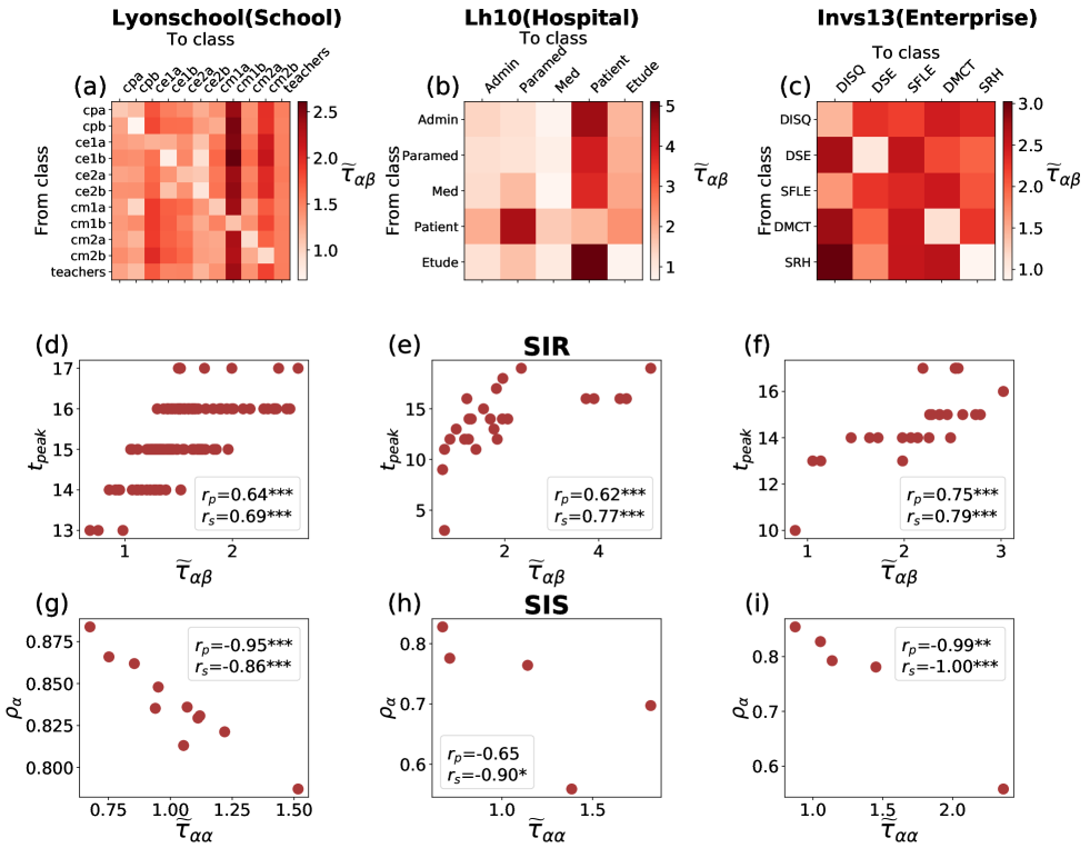
Figure 5: Class mean first passage times and the spread of epidemics in contact networks. (a)-(c) Class mean first passage times in contact networks corresponding to a school, a hospital and an enterprise. (d)-(f) Connection between $\widetilde{\tau}_{\alpha\beta}$ and the time steps until the peak of the epidemic $t_{peak}$ in a SIR model. (g)-(i) Connection between the return times $\widetilde{\tau}_{\alpha\alpha}$ and the fraction of infected individuals in each class in the stationary state. Simulations were performed using the parameters $\beta=0.7$ and $\mu=0.1$.

In Fig. 4(d)-(e), we show the evolution of the average $\widetilde{\tau}_{\alpha\beta}$ between the two main US parties in both the Senate and the House of Representatives. The dashed lines indicate the intra-class MFPT, and indeed support the intuition that polarisation has increased dramatically in recent years. The plots of return times $\widetilde{\tau}_{\alpha\alpha}$ instead (solid lines), are far more stable, and the small oscillations we observe depend only on which is the ruling party, since that one will normally yield lower values of $\widetilde{\tau}_{\alpha\alpha}$.

We quantify the overall polarisation in the Senate and the US House of Representatives by computing the average between the inter-class passage times $(\widetilde{\tau}_{D\to R}+\widetilde{\tau}_{R\to D})/2$, which provides an estimate of how close are the voting behaviours of the two main parties in each Congress. The temporal evolution of $(\widetilde{\tau}_{D\to R}+\widetilde{\tau}_{R\to D})/2$ is shown in Fig. 4(f), where each point is coloured according to the party holding the majority of seats in that term. Again, we observe a clear increase of polarisation after the 1970s in both branches of the Congress, which is in very good agreement with prior works [20, 21, 22]. Notice that there are some interesting patterns there, like for instance the term starting in January 2001, which displays the lowest polarisation in the last 25 years, most likely due to the 9/11 terrorist attacks later that year.

We inspect next if, as hypothesised, the increasing polarisation observed in Fig. 4(f) is due to the party holding the majority of seats in each term. We computed the ratio of inter-class passage times $\widetilde{\tau}_{Maj\to Min}/\widetilde{\tau}_{Min\to Maj}$, where $\widetilde{\tau}_{Maj\to Min}$ is the normalised inter-class MFPT from the party with the majority to the party with the minority and $\widetilde{\tau}_{Min\to Maj}$ is the normalised inter-class MFPT from the minority to the majority. The values of $\widetilde{\tau}_{Maj\to Min}/\widetilde{\tau}_{Min\to Maj}$ (Fig. 4(g)) are indeed relatively stable over time, with the vast majority of points lying along or above the solid grid line corresponding to absence of polarisation. This indicates that in most of the terms over the last 80 years the party holding the majority has been the main driver of polarisation. These results demonstrate that $\widetilde{\tau}_{\alpha\beta}$ is indeed a robust measure of polarisation. We argue that the same framework could be easily used in other contexts, including the polarisation of discussions in (online) social networks [23, 24] or the flip of candidates between different political parties [25]. In particular, it could be also possible to identify those agents or individuals who contribute more to polarisation by looking at the ranking of nodes by their values of CMFPT to other classes.

V Contact assortativity and relation with epidemics spreading

Understanding the mixing between groups of individuals in a network can provide a lot of information about the properties of social dynamics, including the role played by different individuals in the transmission of diseases [26, 1, 27, 28]. As a second case study, we use CMFPTs to identify how different groups of people interact in three face-to-face contact networks, namely the contacts in a hospital, in a school, and in an enterprise, obtained from the SocioPatterns project data set [29, 1, 30, 31].

The definition of groups or classes is specific of each system, e.g., the role of a person in the case of hospitals, the class in the case of schools, and the department in which a person works for the network of contacts in an enterprise environment. The weight of the undirected edge connecting two nodes in each graph is equal to the number of contacts between the corresponding individuals. By looking at the dynamics of two simple epidemic models, namely a Susceptible-Infected-Susceptible (SIS) and a Susceptible-Infected-Recovered (SIR), we show here that the distribution of CMFPT in each graph provides relevant information about the dynamics of disease spreading in the system. For both epidemic models, if an individual $i$ is infected it selects one of its neighbours $j$ with probability $w_{ij}/\sum_{j}w_{ij}$ and infects it with a probability $\beta$. Afterwards, each of the infected individuals will either recover with probability $\mu$ in the case of the SIR model, or become susceptible again in the case of the SIS model.

In Fig. 5(a)-(c) we report the matrices of $\widetilde{\tau}_{\alpha\beta}$ respectively for the school, the enterprise, and the hospital. In the school network, we observe a consistent pattern of lower values of normalised intra-CMFPT $\widetilde{\tau}_{\alpha\alpha}$, which is most probably due to the much higher number of contacts among individuals in the same classroom compared to individuals in other classrooms. Notwithstanding this general pattern, some of the classes are more tightly connected than other close-by classes, as in the case of ce1b and ce2b. Also in the case of the enterprise network we distinguish a clear pattern where for each class $\alpha$ the value of $\widetilde{\tau}_{\alpha\alpha}$ is normally much smaller than $\widetilde{\tau}_{\alpha\beta}$ for $\alpha\neq\beta$. Yet, there are some interesting deviations, as in the case of SFLE. This department plays a similar role to that of teachers in the case of the school network (i.e., contain people that tend to interact with more than one class), and all the other departments exhibit similar values of inter-CMFPT to that class. Finally, in the hospital contact network patients seem to be the most isolated, while the paramedical staff and display lower CMFPT to all the other classes.

As we show in the following, we found a quite interesting relation between the pattern of CMFPT in each network and the spreading dynamics on the same graph. We run a large number of simulations of the SIR and SIS models, seeding the disease in each of the nodes of a network, and calculating the number of time-steps needed to the spread to reach the peak in each of the classes, as a function of the group to which the seed node belongs. In Fig. 5(d)-(f) we report, as a function of $\widetilde{\tau}_{\alpha\beta}$, the average number of steps until the peak of the epidemic $t_{peak}$ in class $\beta$ is reached in a SIR model where the seed is a node in class $\alpha$. Interestingly, we found that the time to the peak in class $\beta$ is an increasing function of $\widetilde{\tau}_{\alpha\beta}$, and the rank correlation between the two variables is always pretty large and significant in the three systems.

The results on the SIS model somehow complement the picture observed in the case of SIR. In Fig. 5(g)-(i) we show that the class mean return times $\widetilde{\tau}_{\alpha\alpha}$ are strongly correlated with the fraction $\rho_{\alpha}$ of infected individuals of that class in the stationary state. In particular, the lower the value of $\widetilde{\tau}_{\alpha\alpha}$, the larger the fraction of infected individuals in class $\alpha$ in the endemic state, suggesting that the steady-state dynamics is indeed predominantly driven by interactions among individuals in the same class. In Table 2 we report these correlations for a wider range of $\beta$ and $\mu$. As shown in detail in Fig. 7 and Fig. 8, the observed correlations between $\rho_{\alpha}$ and $\tau_{\alpha\beta}$ are consistently higher than the correlation with either the total number of edges between two classes or the total fraction of edges from class $\alpha$ to class $\beta$. Those results as well as the correlations with a wider range of parameters and contact networks can be found in Appendix B.

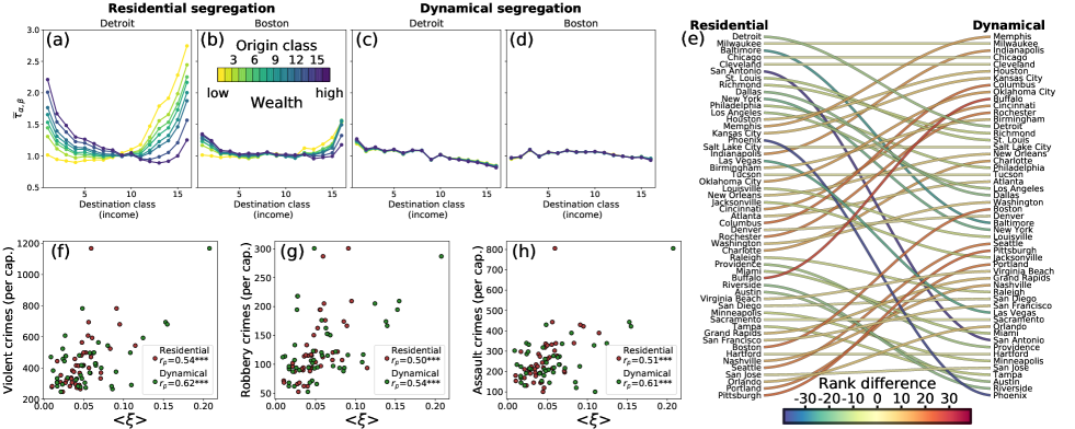
Figure 6: Class mean first passage times and urban income inequality. (a)-(d) Class mean first passage times $\widetilde{\tau}_{\alpha\beta}$ between each of the income categories in Detroit and Boston when computed over the (a,b) adjacency (residential segregation) and the (c,d) commuting graphs (dynamical segregation. (e) Changes in the ranking of values between the residential and dynamical segregation. (f)-(h) Correlation between the index of segregation $\langle\xi\rangle$ and the criminality in US cities. (f) Violent crimes, (g) robbery crimes and (h) assault crimes.

VI Residential and dynamical urban economic segregation

Socio-economic segregation has an enormous impact on city livability, and many different measures to quantify it have been proposed in the past years. However, most of those measures, with a few notable exceptions [32], focus on first-neighbour information, and disregard the role of the mobility of citizens [33, 34, 35, 36]. We test here the potential of CMFPTs to quantify urban economic segregation in large metropolitan areas, taking into account the daily mobility patterns of individuals.

We considered the $53$ US cities with more than one million inhabitants, and census information about the number of households in each of the 16 income categories defined by the US Census Borough (see Table 3 and the 2017 American Community survey [37]), where class 1 is lowest income and class 16 is the highest one. We constructed two different graphs among census tracts, namely the graph of tract adjacency and the graph of daily workplace commuting [38]. The former graph is undirected and unweighted, and is better suited to measure the so-called residential segregation, i.e., the extent to which people with similar levels of income tend to live in close-by areas. The commuting graph, instead, is directed and weighted so that the weight of a link going from $i$ to $j$ is given by the sum of the residents in $i$ working in $j$ and the residents of $j$ working in $i$ in order to mimick the daily mobility of citizens.

The fact that households of more than one category are present in each block group prevents us from assigning a single class to each unit, so we computed the distribution of CMFPT by averaging over a large number of realisations of class assignments. In each realisation, the class of each node in the graph is sampled from the distribution of household in the corresponding census tract, so that the probability that node $i$ is assigned to class $\alpha$ in a given realisation is equal to $m_{i,\alpha}/\sum_{\forall\beta}m_{i,\beta}$, where $m_{i,\alpha}$ is the number of people of category $\alpha$ living in node $i$. We took a slightly different approach for the commuting graph as described in [39], where the population attributed to node $i$ is a combination of the resident population at $i$ and the number of commuters working at $i$:

$$\widetilde{m}_{i,\alpha}=m_{i,{\alpha}}+\sum_{j}\omega_{ji}\frac{m_{j,{\alpha}}}{\sum_{\forall\beta}m_{j,\beta}},$$ (14)

where $\omega_{ji}$ is the weight from node $j$ to node $i$ in the commuting graph, which is equal to the total number of people who live in $j$ and commute to their workplace in $i$. By doing so we take into account the fact that commuters effectively contribute to the diversity of an area, as they spend a considerable amount of time in there and actually interact with other commuters coming from different areas as well. For each realisation of a class assignment, we run $10^{4}-10^{6}$ random walkers from each of the nodes. Then, we obtain the CMFPT $\tau_{\alpha\beta}$ for each ordered pairs of classes ($\alpha,\beta$) by averaging over all nodes and realisations of class assignments, and we analyse the normalised CMFPT $\widetilde{\tau}_{\alpha\beta}=\tau_{\alpha\beta}/\tau^{\rm null}_{\alpha\beta}$.

In Fig. 6(a)-(b) we show the profiles of $\widetilde{\tau}_{\alpha\beta}$ from each of the 16 classes computed over the adjacency graph, respectively for Detroit and Boston. It is worth noting that the categories at the two extremes (i.e., the poorest and the wealthiest ones) exhibit a quite similar pattern in the two cities. They are both characterised by larger values of CMFPT from any of the other classes, meaning that those two classes are in general more isolated from the rest of the population, with most of the high-income classes appearing slightly more isolated in Detroit than in Boston. Moreover, in both cities all classes have a virtually identical value of CMFPT to class 9, and very similar values to class 8 and 10, which indicates that these middle-income classes play a pivotal role in the spatial distribution of income. However, despite the fact that the qualitative behaviour is similar in the two cities, there are some noticeable quantitative differences. First of all, the values of normalised CMFPT are significantly larger in Detroit than in Boston. Second, in Detroit we observe a strong dependence of CMFPT on the class of the starting node, while in Boston the average number of steps required to reach a class below 12 is almost constant regardless of the category of the origin node. These important quantitative differences would suggest that the spatial distribution of income in Detroit is more heterogeneous than in Boston, a conclusion which is in line with the classical literature about economic segregation in the US [40, 41, 42, 3].

However, in large metropolitan areas most of the daily activities of individuals happen far away from their home, due to urbanisation pressure and to decentralisation of productive sectors, so that residential segregation can hardly tell the whole story. Indeed, in the last years there has been an increasing interest in the quantification of social and economic segregation by taking into account mobility patterns [43, 44, 45]. This is easily doable within our framework by letting the walkers move on the mobility graph instead of the adjacency network between census tracts. We have computed $\widetilde{\tau}_{\alpha\beta}$ upon the mobility graph of each US city in the data set, as obtained from workplace commuting information. The results are shown in Fig. 6(c)-(d), and provide an interesting picture of the differences between residential and mobility-focused segregation. First of all, in both cities $\widetilde{\tau}_{\alpha\beta}$ does not depend too much on the origin class $\alpha$ but instead on the destination class $\beta$. This is most likely due to the fact that people of different backgrounds commute to similar areas – i.e. the city centre and industrial sites–. Still, both cities display a distinct organisation of CMFPTs. In Detroit low income classes are much more isolated (higher $\widetilde{\tau}_{\alpha\beta}$) compared to high income classes, which exhibit systematically lower values of $\widetilde{\tau}_{\alpha\beta}$. In the case of Boston, instead, $\widetilde{\tau}_{\alpha\beta}$ is almost flat with no important dependence on either the source or the destination class.

The profiles of $\widetilde{\tau}_{\alpha\beta}$ that we show in Fig. 6(a)-(d) provide an overall clear picture of the distribution of CMFPT in a metropolitan area, but do not allow to easily compare two cities in a systematic manner. Hence, we devised two synthetic indices $\overline{\xi^{out}}$ and $\overline{\xi^{in}}$ that summarise the information on spatial income heterogeneity in a single number. The idea behind these quantities is that an income class $\alpha$ is more heterogeneously distributed if there is a large difference between the CMFPT from $\alpha$ to the income classes immediately adjacent to $\alpha$ and the median CMFPT from $\alpha$ to any other class. We consider the discrepancy between the local and global median of CMFPT from class $\alpha$:

$$\xi^{out}_{\alpha}=|\overline{\widetilde{\tau}}_{\alpha_{nn}}^{\rm out}-\overline{\widetilde{\tau}}^{\rm out}_{\alpha}|$$

where $\overline{\widetilde{\tau}}^{out}_{\alpha}$ is the median of $\widetilde{\tau}_{\alpha\beta}$ when $\alpha\neq\beta$ and $\overline{\widetilde{\tau}}_{\alpha_{nn}}^{\rm out}$ is the median of $\widetilde{\tau}_{\alpha\beta}$ to its nearest neighbours $\beta\in\{\alpha-1,\alpha,\alpha+1\}$  Similarly for the discrepancy between local and global median of CMFPT to class $\alpha$:

$$\xi^{in}_{\alpha}=|\overline{\widetilde{\tau}}_{\alpha_{nn}}^{\rm in}-\overline{\widetilde{\tau}}^{\rm in}_{\alpha}|$$

where $\overline{\widetilde{\tau}}^{\rm in}_{\alpha}$ and $\overline{\widetilde{\tau}}_{\alpha_{nn}}^{\rm in}$ are now the median of $\widetilde{\tau}_{\beta\alpha}$ when $\alpha\neq\beta$ and the median of $\widetilde{\tau}_{\beta\alpha}$ from its nearest neighbours $\beta\in\{\alpha-1,\alpha,\alpha+1\}$, respectively.

In Fig. 6(e) we show the ranking of US cities induced by $\langle\xi\rangle=(\overline{\xi^{in}}+\overline{\xi^{out}})/2$, that is the average discrepancy between local and global CMFPT from/to each income class. In general, larger values of $\langle\xi\rangle$ indicate more pronounced levels of segregation. On the left-hand side of the panel the cities are ranked according to $\langle\xi\rangle$ in the adjacency graph of census tracts, while on the right-hand side the ranking is based on $\langle\xi\rangle$ in the commuting graph. Interestingly, Detroit is the first US city by residential segregation, with other cities traditionally known for their high levels of segregation like Milwaukee and Cleveland following closely. Conversely, Boston is at the bottom of the ranking. However, the ranking changes substantially if we consider instead the mobility graph, and what we call dynamic segregation, as reported in the right-hand side of Fig. 6(e). For instance, Baltimore (which is ranked pretty high for residential segregation) gets relegated to a mid-rank position, while cities like Buffalo or Indianapolis, where residential segregation is not that high, get to the top of the ranking of dynamic segregation.

The most interesting aspect of $\langle\xi\rangle$ is that it captures some of the most undesirable consequences of income segregation, namely the incidence of different types of crimes obtained from [47]. In Fig. 6(f)-(h) we report the correlation between incidence per-capita of assaults, violent crimes, and robberies with the levels of residential segregation measured on the adjacency and on the commuting graph of the cities in our data set. Interestingly, both indices display a significant correlation with all three types of crime. Moreover, the indices computed over the commuting network display a stronger correlation in all three cases, reinforcing the idea that quantifying segregation by disregarding mobility can indeed lead to distorted conclusions. For instance, the city that appears on the top of the dynamical segregation ranking (Memphis) is the one displaying the highest incidence of violent crimes per-capita among the largest US cities, although it is placed in the second quartile of the ranking by residential segregation. As a comparison, we report in Appendix C the correlations of traditional metrics of segregation (i.e., the Spatial Gini coefficient and the Moran’s I index) with the same crime indicators, showing that they are not able to attain values as high as those obtained with $\langle\xi\rangle$. Besides the lower correlations, it is also important to note that both the Spatial Gini Coefficient and the Moran’s I index are symmetric quantities, and as such they fail to capture the intrinsic asymmetry between income classes revealed by Fig. 6(a)-(d).

Overall, our methodology based on the diffusion of random walks is not only a natural extension of the latter multi-scalar approaches introduced to characterise residential segregation [48], but it also allows us to define a dynamical segregation that includes mobility into the analysis as it has been recently discussed for instance in Refs. [49, 45].

VII Conclusions

Although being a relatively simple and intuitive tool, random walks have been extensively and successfully used to model and characterise transportation [50, 51], biological [52, 53], and financial systems [54]. They have proven useful to detect meaningful structural properties in complex networks [14, 55], including communities [56, 57, 58], node roles [59], navigability [60], and temporal variability [61]. Moreover, interesting insights about the relation between the structure and dynamics on a network have come from the analysis of transient and long trajectories of random walks on graphs, including the statistics of first passage times and coverage times [13, 62, 63, 64, 12], or the systematic study of their fluctuations [65]. However, the potential usefulness of random walks to quantify the heterogeneity of class distributions on networks, either in spatially-embedded systems or in high-dimensional networks, has only recently been hinted to [65, 39, 66].

We have shown here that the information captured by the distribution of inter-class mean first passage times can be used not just as a way to detect the presence of anisotropy and correlations in the properties of nodes, but also as a reliable proxy for the dynamics and emergent behaviours of a complex system. One of the most interesting aspects of the measures of heterogeneity, polarisation, and segregation that we have introduced in this work is that they take into account microscopic, meso-scopic and global relations among classes, due to the fact that in principle random walks integrate information about paths of all possible lengths. Another relevant property of the measures of segregation based on CMFPT is that they are non-parametric and correctly normalised with respect to a meaningful null-model, hence allowing us to compare on equal grounds the heterogeneity of class distributions in systems of different sizes, which is where most of the classical indices of segregation fail [34, 48]. Even more importantly, the profiles of inter-class mean-first passage times are not symmetric with respect to classes, and provide fine-grained information about which classes are most responsible for the emergence of polarisation and heterogeneity. In this respect, it would be worthy exploring how the simple measure of polarisation that we proposed can be extended to the case of more than two classes.

The fact that measures of class heterogeneity based on random walk statistics correlate quite well with some of intrinsic dynamics happening in social network (i.e., the spread of an epidemic) and with some other exogenous processes mediated by the underlying graph (i.e., the incidence of crime in a city) confirm that the profiles of CMFPT are a useful toolbox for targeted mitigation of the undesired effects of these dynamics. For instance, the groups of a social network that are more central according to $\widetilde{\tau}_{\alpha\beta}$ might be the best candidates for early vaccinations to slow-down an epidemic. At the same time, the definition of dynamical segregation based on walks on the mobility graphs, and the fact that it correlates quite substantially with crimes, potentially paves the way for a re-definition of the traditional role attributed to residential segregation, in favour of a more balanced view that takes into account the activity patterns of citizens together with the spatial distribution of their dwellings.

The generality of the methodology proposed in this paper, and its applicability to different classical problems in complexity science, establish a concrete link between classical statistical physics and modern complexity science, and have the potential to provide new interesting insights about the relation between structure and dynamics of complex systems.

Appendix A Derivation of CMFPT in simple geometries

A.1 Chain of nodes

We derive the full distribution of CMFPT for the chain of nodes depicted in Fig. 2(b), as a function of the length $L$ of the chain. For $L\geq 6$ the forward equations for the mean first passage time to blank nodes read:

$$T_{0,\bullet}=1+\frac{1}{4}T_{1,\bullet}$$ (15)

$$T_{M-k,\bullet}=1+\frac{1}{4}\left[T_{M-k+1,\bullet}+T_{M-k-1,\bullet}\right],\quad k=1,2,\ldots,M-1$$ (16)

$$T_{M,\bullet}=\left\{\begin{aligned} &\frac{4}{3}+\frac{1}{3}T_{M-1,bl}\quad\quad{\rm if}a\>L\>{\rm is\>even}\\ &1+\frac{1}{2}T_{M-1,\bullet}\quad\quad{\rm if}\>L\>{\rm is\>odd}\end{aligned}\right.$$ (17)

By iteratively substituting $T_{M-k+1}$ into Eq. (16) for $k=1,2,\ldots$ we find a parametric recursive expression for $T_{M-k,0}$:

$$T_{M-k,\bullet}=A_{k}+B_{k}T_{M-k-1,\bullet}$$ (18)

Although the two sequences $A_{k}$ and $B_{k}$ depend on whether $L$ is even or odd, as we explain below, it is possible to derive a generic solution for this set of recurrence equations. In particular, we write Eq. (18) for $k=M-1$:

$$T_{M-(M-1),\bullet}=T_{1,\bullet}=A_{M-1}+B_{M-1}T_{0,\bullet}$$ (19)

and we substitute it in Eq. 15 to obtain:

$$T_{0,\bullet} =1+\frac{1}{4}T_{1,\bullet}=1+\frac{1}{4}\left[A_{M-1}+B_{M-1}T_{0,\bullet}\right]$$

$$\Rightarrow T_{0,\bullet}=\frac{4+A_{M-1}}{4-B_{M-1}}$$ (20)

By plugging Eq. (20) into Eq. (19), and then recursively propagating back the result in Eq. (18), we obtain a closed expression for $T_{k,\bullet}$ when $k=0,1,\ldots M-1$:

$$T_{k,\bullet}=\left[\frac{4+A_{M-1}}{4-B_{M-1}}\right]\prod_{\ell=1}^{k}B_{M-\ell}+\sum_{j=1}^{k-1}A_{M-k+j}\prod_{\ell=0}^{j-1}B_{M-k+\ell}$$ (21)

which together with Eq. (17) provides the entire distribution of $T_{k,\bullet}$ across the chain. As we mentioned above, the actual form of $A_{k}$ and $B_{k}$ depends on whether the number of nodes $L$ in the chain is even or odd. If $L$ is even we have:

$$A_{k} =\frac{4a_{k}}{b_{k+1}}$$

$$B_{k} =\frac{b_{k}}{b_{k+1}}$$

where

$$a_{k} =\{1,4,15,56,209,\ldots\}$$

$$b_{k} =\{1,3,11,41,153,\ldots\}.$$

It is easy to prove that both $a_{k}$ and $b_{k}$ satisfy the recurrent relation:

$$x_{n}=4x_{n-1}-x_{n-2},\quad n=0,1,\ldots$$ (22)

with slightly different initial conditions. By solving these recurrent relations we obtain the closed forms:

$$a_{k} =\frac{\sqrt{3}+2}{2\sqrt{3}}(2+\sqrt{3})^{k}+\frac{\sqrt{3}-2}{2\sqrt{3}}(2-\sqrt{3})^{k}$$ (23)

$$b_{k} =\frac{\sqrt{3}+1}{2\sqrt{3}}(2+\sqrt{3})^{k}+\frac{\sqrt{3}-1}{2\sqrt{3}}(2-\sqrt{3})^{k}$$ (24)

which can be used to compute directly the values of $A_{k}$ and $B_{k}$;

In the case of odd length $L$, instead, we obtain:

$$A_{k} =\frac{c_{k}e_{k}}{d_{k}f_{k}}$$

$$B_{k} =\frac{e_{k}}{4f_{k}}$$

where:

$$c_{k} =\{8,28,104,388,1448,\ldots\}$$

$$d_{k} =\{7,26,97,362,1351,\ldots\}$$

$$e_{k} =\{5,19,71,265,989,\ldots\}$$

$$f_{k} =\{4,14,52,194,724,\ldots\}$$

Also these four sequences satisfy the general recurrence relation in Eq. (22), and by solving the relation for each of the corresponding initial conditions we obtain the closed forms:

$$c_{k} =\frac{8\sqrt{3}+12}{2\sqrt{3}}(2+\sqrt{3})^{k}+\frac{8\sqrt{3}-12}{2\sqrt{3}}(2-\sqrt{3})^{k}$$ (25)

$$d_{k} =\frac{7\sqrt{3}+12}{2\sqrt{3}}(2+\sqrt{3})^{k}+\frac{7\sqrt{3}-12}{2\sqrt{3}}(2-\sqrt{3})^{k}$$ (26)

$$e_{k} =\frac{5\sqrt{3}+9}{2\sqrt{3}}(2+\sqrt{3})^{k}+\frac{5\sqrt{3}-9}{2\sqrt{3}}(2-\sqrt{3})^{k}$$ (27)

$$f_{k} =\frac{4\sqrt{3}+6}{2\sqrt{3}}(2+\sqrt{3})^{k}+\frac{4\sqrt{3}-6}{2\sqrt{3}}(2-\sqrt{3})^{k}$$ (28)

The cases where $1\leq L<6$ must be considered separately. If $L=1$, then the chain degenerates in a single white node surrounded by four black nodes. In this case, we simply have $T_{0,\bullet}=1$. If $L=2$, instead, the chain contains only two nodes, and is equivalent to the minimal weighted graph shown below:

where for convenience we have shown only the links coming out of white nodes. The forward equation for node $0$ gives:

$$T_{0,\bullet} =1+\frac{1}{4}T_{0,\bullet}$$

$$\Rightarrow T_{0,\bullet}=\frac{4}{3}$$

The case $L=3$ is equivalent to the minimal graph:

and the two mean first passage times to black nodes satisfy the system of equations:

$$\left\{\begin{array}[]{rl}T_{0,\bullet}&=1+\frac{1}{4}T_{1,\bullet}\\ T_{1,\bullet}&=1+\frac{1}{2}T_{0,\bullet}\\ \end{array}\right.$$ (29)

whose unique solution is:

$$T_{0,\bullet}=\frac{10}{7},\quad\quad T_{1,\bullet}=\frac{12}{7}$$ (30)

When $L=4$, the minimal weighted graph reduces to:

and the two mean first passage times satisfy the equations:

$$\left\{\begin{array}[]{rl}T_{0,\bullet}&=1+\frac{1}{4}T_{1,\bullet}\\ T_{1,\bullet}&=1+\frac{1}{4}\left(T_{0,\bullet}+T_{1,\bullet}\right)\\ \end{array}\right.$$ (31)

whose solution is:

$$T_{0,\bullet}=\frac{16}{11},\quad\quad T_{1,\bullet}=\frac{20}{11}$$ (32)

Finally, for $L=5$ the minimal weighted graph is:

which corresponds to the following system of equations:

$$\left\{\begin{array}[]{rl}T_{0,\bullet}&=1+\frac{1}{4}T_{1,\bullet}\\ T_{1,\bullet}&=1+\frac{1}{4}\left(T_{0,\bullet}+T_{2,\bullet}\right)\\ T_{2,\bullet}&=1+\frac{1}{2}T_{1,\bullet}\end{array}\right.$$ (33)

and yields:

$$T_{0,\bullet}=\frac{19}{13}\quad\quad T_{1,\bullet}=\frac{24}{13}\quad\quad T_{2,\bullet}=\frac{25}{13}\quad\quad$$ (34)

A.2 Infinite cylinder

The distribution of CMFPT from white nodes to blank ones in the infinite cylinder is derived by induction on the generic term $T_{M-k,\bullet},\quad k=0,1,\ldots M$. In particular, when $k=0$ we obtain the mean first-passage time from the farthest node $M$, whose forward equation is:

$$T_{M,\bullet}=1+\frac{2}{3}T_{M,\bullet}+\frac{1}{3}T_{M-1,\bullet}$$ (35)

which leads to:

$$T_{M,\bullet}=3+T_{M-1,\bullet}$$ (36)

which in turn depends only on $T_{M-1,\bullet}$. If we now plug this expression in the forward equation for $T_{M-1,\bullet}$:

$$T_{M-1,\bullet}=1+\frac{1}{2}T_{M,\bullet}+\frac{1}{2}T_{M-2,\bullet}$$ (37)

we obtain:

$$T_{M-1,\bullet}=7+T_{M-2,\bullet},$$ (38)

which in turn depends only on $T_{M-2,\bullet}$. By considering the first few terms of this sequence:

$$T_{M-1,\bullet} =7+T_{M-2,\bullet}$$

$$T_{M-2,\bullet} =11+T_{M-3,\bullet}$$

$$T_{M-3,\bullet} =15+T_{M-4,\bullet}$$

$$T_{M-4,\bullet} =19+T_{M-5,\bullet}$$

we realise that the generic term $T_{M-k,\bullet},\quad k=0,1,\ldots M-1$ satisfies the recurrence equation:

$$T_{M-k,\bullet}=(4k+3)+T_{M-k-1,\bullet}.$$ (39)

Notice that the forward equation for $T_{0,\bullet}$ is somehow simpler, and reads:

$$T_{0,\bullet}=1+\frac{1}{2}T_{0,\bullet}+\frac{1}{4}T_{1,\bullet}$$

which can be rewritten as:

$$T_{0,\bullet}=2+\frac{1}{2}T_{1,\bullet}.$$ (40)

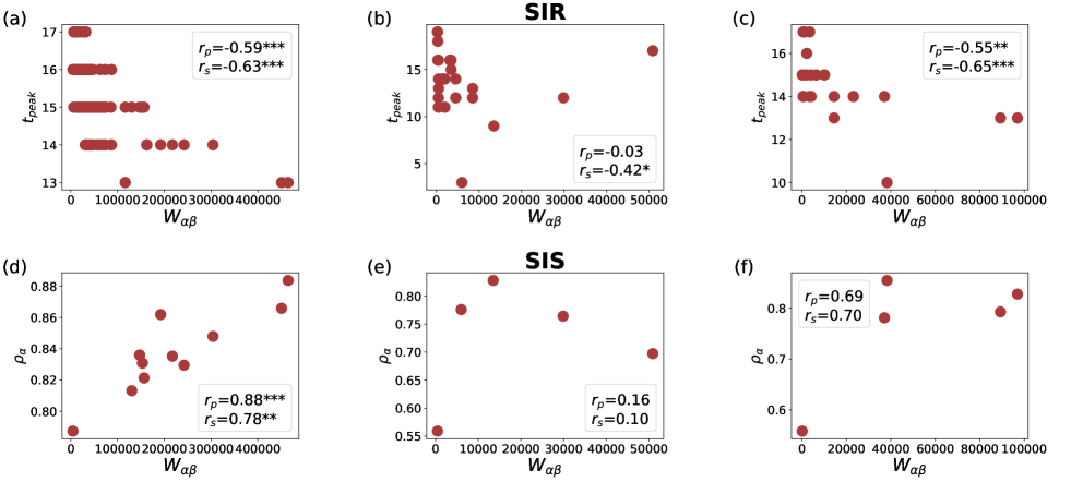
Figure 7: Epidemic spreading in contact networks and inter-group contacts. (a)-(c) Connection between the total number of contacts between classes and the time steps until the peak of the epidemic in a SIR model. (d)-(f) Connection between the total number of contacts within each class and the fraction of infected individuals in each class in the stationary state.

If we now consider Eq. (39) for $k=M-1$:

$$T_{1,\bullet}=4(M-1)+3+T_{0,\bullet}$$ (41)

and we plug it into Eq. (40), we get:

$$T_{0,\bullet}=2+\frac{1}{2}\left[4(M-1)+3+T_{0,\bullet}\right]$$ (42)

which can be solved for $T_{0,\bullet}$, yielding:

$$T_{0,\bullet}=4M+3.$$ (43)

By substituting $T_{0,\bullet}$ back in Eq. (41), and recursively using the results to obtain $T_{2,\bullet},T_{3,\bullet},\ldots$, it is easy to find that:

$$T_{k,\bullet}=(k+1)(4M+3-2k),\quad k=0,1,\ldots M-1$$ (44)

and

$$T_{M,\bullet}=3+M(5+2M)$$ (45)

$\Box$.

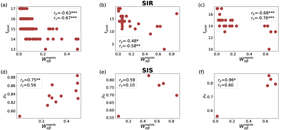
Figure 8: Epidemic spreading in contact networks and inter-group normalised contacts. (a)-(c) Connection between the normalised contacts between classes and the time steps until the peak of the epidemic in a SIR model. (d)-(f) Connection between the normalised contacts within each class and the fraction of infected individuals in each class in the stationary state.

Appendix B Supplementary results for the epidemic spreading in contact networks

We report here the correlation between some simple structural measures and the same epidemic variables considered in Fig. 5. In particular, we have considered two main quantities, namely, the total number of contacts between individuals of group $\alpha$ and group $\beta$ and the normalised contacts of the members of group $\alpha$ with those of group $\beta$. The first quantity is symmetric and is just the sum of the total number of contacts between the members:

$$W_{\alpha\beta}=\sum_{ij}w_{ij}\delta_{f_{i},\alpha}\delta_{f_{j},\beta},$$ (46)

while the second one:

$$W^{\rm norm}_{\alpha\beta}=\frac{W_{\alpha\beta}}{\sum_{\beta}W_{\alpha\beta}},$$ (47)

is normalised by the total number of contacts of the group of origin and, therefore, is in general not symmetric.

In Fig. 7 we show the correlation between the total number of steps until the peak and the total number of contacts between each pair of groups, as well as the correlation between the fraction of population in each group infected in the endemic state (SIS model) and the total contacts between members of the same group. Despite correlations are relatively high and significant in some cases, none of them is higher than those obtained for $\widetilde{\tau}_{\alpha\beta}$.

Similarly, we show in Fig. 8 the correlation of both the SIR and the SIS models with the normalised number of contacts. Correlations look slightly higher than in the case of the total number of contacts, yet they are still considerablu lower than the values obtained for $\widetilde{\tau}_{\alpha\alpha}$. Particularly in the case of the SIS model (stationary dynamics), we do not observe the clear alignment that appears in Fig. 5.

In Fig. 5 we reported the correlation coefficients for only $3$ of the $7$ contact networks we have analysed. Table 2 includes additional results of Pearson’s $r_{p}$ and Spearman’s $r_{s}$ for many combinations of the parameters and a for wider variety of contact networks. Interestingly, the results are compatible with those reported in Fig. 5, and confirm that correlations between CMFPT and critical epidemiological variable are large and significative.

$\beta$	$\mu$	Network	Model	Pearson’s $r_{p}$	Spearman’s $r_{s}$	Model	Pearson’s $r_{p}$	Spearman’s $r_{s}$
0.5	0.1	Thiers13	SIR	0.92***	0.85***	SIS	-0.30	-0.67*
0.5	0.1	InVS15	SIR	0.47***	0.73***	SIS	-0.86***	-0.89***
0.5	0.1	LH10	SIR	0.70***	0.86***	SIS	-0.67	-0.90*
0.5	0.1	InVS13	SIR	0.29	0.73***	SIS	-0.99**	-1.00***
0.5	0.1	Hospital	SIR	0.89***	0.94***	SIS	-0.89	-1.00***
0.5	0.1	Enterprise	SIR	0.59**	0.71***	SIS	-0.95*	-0.70
0.5	0.1	LyonSchool	SIR	0.69***	0.73***	SIS	-0.96***	-0.89***
0.5	0.3	Thiers13	SIR	0.88***	0.79***	SIS	-0.62	-0.73*
0.5	0.3	InVS15	SIR	0.33***	0.37***	SIS	-0.27	-0.52
0.5	0.3	LH10	SIR	0.57**	0.59**	SIS	-0.95*	-0.90*
0.5	0.3	InVS13	SIR	0.68***	0.70***	SIS	-0.54	-0.90*
0.5	0.3	Hospital	SIR	0.30	0.50*	SIS	-0.97*	-1.00***
0.5	0.3	Enterprise	SIR	0.62***	0.68***	SIS	0.48	0.00
0.5	0.3	LyonSchool	SIR	0.50***	0.55***	SIS	-0.96***	-0.95***
0.9	0.1	Thiers13	SIR	0.93***	0.86***	SIS	-0.20	-0.55
0.9	0.1	InVS15	SIR	0.47***	0.74***	SIS	-0.82**	-0.80**
0.9	0.1	LH10	SIR	0.68***	0.83***	SIS	-0.66	-0.90*
0.9	0.1	InVS13	SIR	0.66***	0.68***	SIS	-0.98**	-1.00***
0.9	0.1	Hospital	SIR	0.77***	0.80***	SIS	-0.87	-0.80
0.9	0.1	Enterprise	SIR	0.51**	0.56**	SIS	-0.95*	-0.70
0.9	0.1	LyonSchool	SIR	0.67***	0.73***	SIS	-0.94***	-0.86***
0.7	0.3	Thiers13	SIR	0.93***	0.87***	SIS	-0.47	-0.63
0.7	0.3	InVS15	SIR	0.28***	0.47***	SIS	-0.67*	-0.59*
0.7	0.3	LH10	SIR	0.65***	0.76***	SIS	-0.84	-0.90*
0.7	0.3	InVS13	SIR	0.52**	0.68***	SIS	-0.98**	-1.00***
0.7	0.3	Hospital	SIR	0.63**	0.83***	SIS	-0.95	-1.00***
0.7	0.3	Enterprise	SIR	0.67***	0.69***	SIS	-0.93*	-0.90*
0.7	0.3	LyonSchool	SIR	0.34***	0.55***	SIS	-0.97***	-0.93***
0.7	0.1	Thiers13	SIR	0.93***	0.86***	SIS	-0.25	-0.67*
0.7	0.1	InVS15	SIR	0.45***	0.72***	SIS	-0.84***	-0.85***
0.7	0.1	LH10	SIR	0.62***	0.77***	SIS	-0.65	-0.90*
0.7	0.1	InVS13	SIR	0.75***	0.79***	SIS	-0.99**	-1.00***
0.7	0.1	Hospital	SIR	0.86***	0.89***	SIS	-0.87	-0.80
0.7	0.1	Enterprise	SIR	0.61**	0.64***	SIS	-0.95*	-0.70
0.7	0.1	LyonSchool	SIR	0.64***	0.69***	SIS	-0.95***	-0.86***
0.9	0.5	Thiers13	SIR	0.89***	0.78***	SIS	-0.56	-0.63
0.9	0.5	InVS15	SIR	0.31***	0.40***	SIS	-0.38	-0.50
0.9	0.5	LH10	SIR	0.58**	0.76***	SIS	-0.92*	-0.80
0.9	0.5	InVS13	SIR	0.62***	0.69***	SIS	-0.89*	-1.00***
0.9	0.5	Hospital	SIR	0.29	0.58*	SIS	-0.97*	-1.00***
0.9	0.5	Enterprise	SIR	0.68***	0.72***	SIS	-0.35	-0.70
0.9	0.3	Thiers13	SIR	0.92***	0.85***	SIS	-0.39	-0.58
0.9	0.3	InVS15	SIR	0.36***	0.64***	SIS	-0.81**	-0.81**
0.9	0.3	LH10	SIR	0.61**	0.77***	SIS	-0.68	-0.90*
0.9	0.3	InVS13	SIR	0.50*	0.71***	SIS	-0.99**	-1.00***
0.9	0.3	Hospital	SIR	0.59*	0.94***	SIS	-0.92	-1.00***
0.9	0.3	Enterprise	SIR	0.65***	0.73***	SIS	-0.96*	-0.70
0.7	0.5	Thiers13	SIR	0.85***	0.73***	SIS	-0.73*	-0.78*
0.7	0.5	InVS15	SIR	0.35***	0.35***	SIS	0.01	-0.41
0.7	0.5	LH10	SIR	0.61**	0.47*	SIS	-0.87	-0.80
0.7	0.5	InVS13	SIR	0.77***	0.61**	SIS	0.64	0.40
0.7	0.5	Hospital	SIR	0.50	0.55*	SIS	-0.89	-0.80
0.7	0.5	Enterprise	SIR	0.64***	0.73***	SIS	0.72	0.10
0.7	0.5	LyonSchool	SIR	0.53***	0.53***	SIS	-0.91***	-0.98***

Table 2: Pearson correlation coefficient $r_{p}$ and Spearman’s rank correlation coefficient $r_{s}$ for the seven contact networks analysed for both the SIR and SIS models.

Appendix C Supplementary results in the analysis of urban inequalities

We report in Table 3 the income intervals that correspond to each of the classes investigated in the case of urban inequalities.

Class	Income	Class	Income
Class 1	Less than $10,000$	Class 9	$45,000$ to $49,999$
Class 2	$10,000$ to $14,999$	Class 10	$50,000$ to $59,999$
Class 3	$15,000$ to $19,999$	Class 11	$60,000$ to $74,999$
Class 4	$20,000$ to $24,999$	Class 12	$75,000$ to $99,999$
Class 5	$25,000$ to $29,999$	Class 13	$100,000$ to $124,999$
Class 6	$30,000$ to $34,999$	Class 14	$125,000$ to $149,999$
Class 7	$35,000$ to $39,999$	Class 15	$150,000$ to $199,999$
Class 8	$40,000$ to $44,999$	Class 16	$200,000$ or more

Table 3: Corresponding income branch of each class or category in US dollars.

C.1 Correlations with traditional segregation indicators

Given the correlations between the index constructed from CMFPT and set of crime indicators in American cities, we have also checked if traditional segregation indicators provide a comparable amount of information. The two main quantities we analysed are the Spatial Gini and the Moran’s I auto-correlation. We used of The Spatial Gini which can be written as

$$SG=\frac{\sum^{N}_{i=1}\sum^{N}_{j=1}(1-w_{ij})|x_{i}-x_{j}|}{2N^{2}<x>},$$ (48)

This metric is designed for binary networks as it is the case for the adjacency graph of census tracts, however it is not defined for non-binary weights as it is the case of the commuting graph. To take into account those weights, we have modified it as

$$SG_{w}=\frac{\sum^{N}_{i=1}\sum^{N}_{j=1}(1-w_{ij}/w_{\rm max})|x_{i}-x_{j}|}{2N^{2}<x>},$$ (49)

where $w_{\rm max}$ corresponds to the maximum weight observed in the network. In the case of the Moran’s I, it is given by

$$I=\frac{N}{\sum_{i}\sum_{j}w_{ij}}\frac{\sum_{i}\sum_{j}w_{ij}(x_{i}-<x>)(x_{j}-<x>)}{\sum_{i}(x_{i}-<x>)^{2}},$$ (50)

which is generally defined for any type of network. However. there is a slight difference between the adjacency and the commuting graph. In the case of the adjacency graph we have used a row normalised approach for the weights so that each cell counts the same in the global average, while for the commuting graph no normalisation was applied so that a cell with more (in)outgoing links will count more. In Fig. 9, we provide the values of both indices for each of the income categories analysed throughout this paper. As can been seen, the behaviour observed is quite comparable to the one in Fig. 6, with the low and high-income classes displaying significantly higher segregation. Moreover, segregation seems to decrease when computed over the commuting graph.

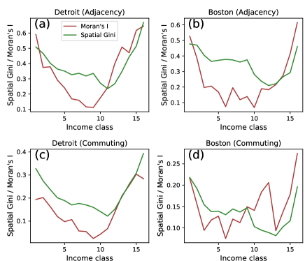
Figure 9: Segregation of each income category with traditional segregation indices when calculated on (a)-(b) the adjacency graph and (c)-(d) the commuting graph

To extract a single metric for each of the cities studied, we have taken the median over all income categories and we have compared the correlations with those observed for the index extracted from CMFPT. We report in Fig. 10 and Fig.11 the correlations for both quantities, the Spatial Gini and the Moran’s I, respectively. While a significant correlation appears in some cases, the highest one observed for the Moran’s I calculated on the adjacency graph is still lower than the lowest correlations observed with our index $\langle\xi\rangle$. This confirms the higher explicative power of a metric based on the diffusion on random walks and the crucial role of including mobility into the analysis.

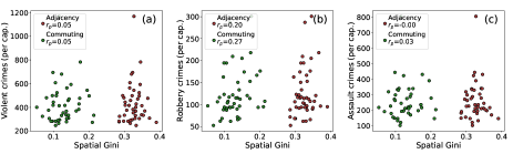
Figure 10: Economic segregation and criminality. (a)-(c) Correlation between the Spatial Gini and the criminality in US cities. (a) Violent crimes, (b) robbery crimes and (c) assault crimes.

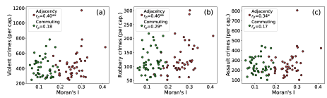
Figure 11: Economic segregation and criminality. (a)-(c) Correlation between the Moran’s I index and the criminality in US cities. (a) Violent crimes, (b) robbery crimes and (c) assault crimes.

References

References

- Vanhems et al. [2013] P. Vanhems, A. Barrat, C. Cattuto, J.-F. Pinton, N. Khanafer, C. Régis, B.-a. Kim, B. Comte, and N. Voirin, PloS one 8, e73970 (2013).
- Fernández-Gracia et al. [2014] J. Fernández-Gracia, K. Suchecki, J. J. Ramasco, M. San Miguel, and V. M. Eguíluz, Physical review letters 112, 158701 (2014).
- Jargowsky [1996] P. A. Jargowsky, American sociological review pp. 984–998 (1996).
- Yan et al. [2017] G. Yan, P. E. Vértes, E. K. Towlson, Y. L. Chew, D. S. Walker, W. R. Schafer, and A.-L. Barabási, Nature 550, 519 (2017), ISSN 1476-4687, URL https://doi.org/10.1038/nature24056.
- Barthelemy [2016] M. Barthelemy, The Structure and Dynamics of Cities: Urban Data Analysis and Theoretical Modeling (Cambridge University Press, 2016).
- Batty [2017] M. Batty, The new science of cities (MIT Press, 2017), ISBN 9780262534567.
- Bullmore and Sporns [2009] E. Bullmore and O. Sporns, Nat Rev Neurosci 10, 186 (2009), ISSN 1471-003X, URL http://dx.doi.org/10.1038/nrn2575.
- Bassett and Sporns [2017] D. S. Bassett and O. Sporns, Nature Neuroscience 20, 353 (2017), ISSN 1546-1726, URL https://doi.org/10.1038/nn.4502.
- Noh and Rieger [2004] J. D. Noh and H. Rieger, Physical review letters 92, 118701 (2004).
- Zhang et al. [2011] Z. Zhang, A. Julaiti, B. Hou, H. Zhang, and G. Chen, The European Physical Journal B 84, 691 (2011).
- Hwang et al. [2012] S. Hwang, D.-S. Lee, and B. Kahng, Physical review letters 109, 088701 (2012).
- Bonaventura et al. [2014] M. Bonaventura, V. Nicosia, and V. Latora, Phys. Rev. E 89, 012803 (2014), URL https://link.aps.org/doi/10.1103/PhysRevE.89.012803.
- Redner [2001] S. Redner, A guide to first-passage processes (Cambridge University Press, 2001).
- Masuda et al. [2017] N. Masuda, M. A. Porter, and R. Lambiotte, Physics Reports 716-717, 1 (2017), ISSN 0370-1573.
- Marcon and Puech [2003] E. Marcon and F. Puech, Journal of Economic Geography 3, 409 (2003).
- Marcon and Puech [2010] E. Marcon and F. Puech, Journal of Economic Geography 10, 745 (2010).
- Braha and De Aguiar [2017] D. Braha and M. A. De Aguiar, PloS one 12, e0177970 (2017).
- Stolz et al. [2016] B. J. Stolz, H. A. Harrington, and M. A. Porter, The topological ”shape” of brexit (2016), eprint 1610.00752.
- Dlotko et al. [2019] P. Dlotko, S. Rudkin, and W. Qiu, An economic topology of the brexit vote (2019), eprint 1909.03490.
- Waugh et al. [2011] A. S. Waugh, L. Pei, J. H. Fowler, P. J. Mucha, and M. A. Porter, arXiv preprint arXiv:0907.3509v3 (2011).
- Hirano et al. [2010] S. Hirano, J. M. Snyder Jr, S. D. Ansolabehere, and J. M. Hansen, Quarterly Journal of Political Science (2010).
- Neal [2020] Z. P. Neal, Social Networks 60, 103 (2020).
- Guerra et al. [2013] P. H. C. Guerra, W. Meira Jr, C. Cardie, and R. Kleinberg, in ICWSM (2013).
- Matakos et al. [2017] A. Matakos, E. Terzi, and P. Tsaparas, Data Mining and Knowledge Discovery 31, 1480 (2017).
- Faustino et al. [2019] J. Faustino, H. Barbosa, E. Ribeiro, and R. Menezes, Applied Network Science 4, 48 (2019).
- Starnini et al. [2013] M. Starnini, A. Machens, C. Cattuto, A. Barrat, and R. Pastor-Satorras, Journal of theoretical biology 337, 89 (2013).
- Barrat et al. [2014] A. Barrat, C. Cattuto, A. E. Tozzi, P. Vanhems, and N. Voirin, Clinical Microbiology and Infection 20, 10 (2014).
- Kiti et al. [2016] M. C. Kiti, M. Tizzoni, T. M. Kinyanjui, D. C. Koech, P. K. Munywoki, M. Meriac, L. Cappa, A. Panisson, A. Barrat, C. Cattuto, et al., EPJ data science 5, 1 (2016).
- Soc [2016] DATASETS SocioPatterns.org, http://www.sociopatterns.org/datasets/ (2016), [Online; accessed 2020-09-30].
- Génois et al. [2015] M. Génois, C. L. Vestergaard, J. Fournet, A. Panisson, I. Bonmarin, and A. Barrat, Network Science 3, 326 (2015), ISSN 2050-1250, URL http://journals.cambridge.org/article_S2050124215000107.
- G’enois and Barrat [2018] M. G’enois and A. Barrat, EPJ Data Science 7, 11 (2018), ISSN 2193-1127, URL https://doi.org/10.1140/epjds/s13688-018-0140-1.
- Barter and Gross [2019] E. Barter and T. Gross, Proceedings of the Royal Society A 475, 20180615 (2019).
- Winship [1977] C. Winship, Social Forces 55, 1058 (1977).
- Reardon and O’Sullivan [2004] S. F. Reardon and D. O’Sullivan, Sociological methodology 34, 121 (2004).
- Ballester and Vorsatz [2014] C. Ballester and M. Vorsatz, The Review of Economics and Statistics 96, 383 (2014), URL https://doi.org/10.1162/REST_a_00399.
- Louf and Barthelemy [2016] R. Louf and M. Barthelemy, PloS one 11, e0157476 (2016).
- [37] S. Manson, J. Schroeder, D. V. Riper, and S. Ruggles, IPUMS National Historical Geographic Information System: Version 14.0 [Database]. Minneapolis, MN: IPUMS. 2019., http://doi.org/10.18128/D050.V14.0.
- Com [2016] Longitudinal Employer-Household Dynamics, https://lehd.ces.census.gov/ (2016), online; accessed 2020-05-30.
- Bassolas et al. [2020a] A. Bassolas, S. Sousa, and V. Nicosia, arXiv preprint arXiv:2007.04130 (2020a).
- Logan [2013] J. R. Logan, City & community 12 (2013).
- pew [2016] The Rise of Residential Segregation by Income — Pew Research Center, https://www.pewsocialtrends.org/2012/08/01/the-rise-of-residential-segregation-by-income/ (2016), online; accessed 2020-05-30.
- Waitzman and Smith [1998] N. J. Waitzman and K. R. Smith, The Milbank Quarterly 76, 341 (1998).
- Le Roux et al. [2017a] G. Le Roux, J. Vallée, and H. Commenges, Journal of Transport Geography 59, 134 (2017a).
- Petrović et al. [2018] A. Petrović, M. van Ham, and D. Manley, Annals of the American Association of Geographers 108, 1057 (2018).
- Randon-Furling et al. [2020] J. Randon-Furling, M. Olteanu, and A. Lucquiaud, Environment and Planning B: Urban Analytics and City Science 47, 645 (2020).
- Note [1] Note1, if or we only consider the median between, respectively, or .
- ucr [2016] Uniform Crime Reporting (UCR) Program — FBI, https://ucr.fbi.gov/crime-in-the-u.s/ (2016), [Online; accessed 2020-09-30].
- Olteanu et al. [2019] M. Olteanu, J. Randon-Furling, and W. A. Clark, Proceedings of the National Academy of Sciences 116, 12250 (2019).
- Le Roux et al. [2017b] G. Le Roux, J. Vallée, and H. Commenges, Journal of Transport Geography 59, 134 (2017b).
- De Domenico et al. [2014] M. De Domenico, A. Solé-Ribalta, S. Gómez, and A. Arenas, Proceedings of the National Academy of Sciences 111, 8351 (2014).
- Bassolas et al. [2020b] A. Bassolas, R. Gallotti, F. Lamanna, M. Lenormand, and J. J. Ramasco, Scientific reports 10, 1 (2020b).
- Codling et al. [2008] E. A. Codling, M. J. Plank, and S. Benhamou, Journal of the Royal Society Interface 5, 813 (2008).
- Nicosia et al. [2017] V. Nicosia, P. S. Skardal, A. Arenas, and V. Latora, Physical review letters 118, 138302 (2017).
- Bacry et al. [2001] E. Bacry, J. Delour, and J.-F. Muzy, Physica A: statistical mechanics and its applications 299, 84 (2001).
- Zhang et al. [2013] Z. Zhang, T. Shan, and G. Chen, Physical Review E 87, 012112 (2013).
- Pons and Latapy [2006] P. Pons and M. Latapy, in J. Graph Algorithms Appl (Citeseer, 2006).
- Rosvall and Bergstrom [2008] M. Rosvall and C. T. Bergstrom, Proceedings of the National Academy of Sciences 105, 1118 (2008).
- Lambiotte et al. [2014] R. Lambiotte, J.-C. Delvenne, and M. Barahona, IEEE Transactions on Network Science and Engineering 1, 76 (2014).
- Newman [2005] M. E. Newman, Social networks 27, 39 (2005).
- De Domenico et al. [2015] M. De Domenico, A. Lancichinetti, A. Arenas, and M. Rosvall, Physical Review X 5, 011027 (2015).
- Hoffmann et al. [2013] T. Hoffmann, M. A. Porter, and R. Lambiotte, in Temporal Networks (Springer, 2013), pp. 295–313.
- Condamin et al. [2005] S. Condamin, O. Bénichou, and M. Moreau, Physical review letters 95, 260601 (2005).
- Condamin et al. [2008] S. Condamin, V. Tejedor, R. Voituriez, O. Bénichou, and J. Klafter, Proceedings of the National Academy of Sciences 105, 5675 (2008).
- Fronczak and Fronczak [2009] A. Fronczak and P. Fronczak, Phys. Rev. E 80, 016107 (2009), URL http://link.aps.org/doi/10.1103/PhysRevE.80.016107.
- Nicosia et al. [2014] V. Nicosia, M. D. Domenico, and V. Latora, EPL (Europhysics Letters) 106, 58005 (2014), URL https://doi.org/10.1209%2F0295-5075%2F106%2F58005.
- Sousa and Nicosia [2020] S. Sousa and V. Nicosia, arXiv preprint arXiv:2010.10462 (2020).