A non-uniform corner-cutting subdivision scheme with an improved accuracy

Byeongseon Jeong §, Hyoseon Yang , and Jungho Yoon § Institute of Mathematical Sciences, Ewha Womans University, Seoul 03760, South Korea (bjeong_ewha@ewha.ac.kr) Department of Computational Mathematics, Science and Engineering, Michigan State University, East Lansing, MI 48824, USA (hyoseon@msu.edu, corresponding author) Department of Mathematics, Ewha Womans University, Seoul 03760, South Korea (yoon@ewha.ac.kr)
Abstract

The aim of this paper is to construct a new non-uniform corner-cutting (NUCC) subdivision scheme that improves the accuracy of the classical (stationary and nonstationary) methods. The refinement rules are formulated via the reproducing property of exponential polynomials. An exponential polynomial has a shape parameter so that it may be adapted to the characteristic of the given data. In this study, we propose a method of selecting the shape parameter, so that it enables the associated scheme to achieve an improved approximation order (that is, three), while the classical methods attain the second order accuracy. An analysis of convergence and smoothness of the proposed scheme is conducted. The proposed scheme is shown to have the same smoothness as the classical Chaikin’s corner-cutting algorithm, that is, C1superscript𝐶1C^{1}. Finally, some numerical examples are presented to demonstrate the advantages of the new corner-cutting algorithm.

keywords:
Corner-cutting Scheme, Exponential B-spline, Nonuniform Subdivision, Approximation Order

1 Introduction

Subdivision schemes are recursive processes of generating smooth curves or surfaces from a given sequence of control points. By applying a set of refinement rules to an initial sequence of points iteratively, a subdivision scheme computes denser sequences of points under a suitable convergence criteria. Due to the algorithmic efficiency in geometric modeling and design, subdivision schemes are extensively studied and utilized in many research fields such as computer-aided geometric design, computer graphics, image processing, scientific computing etc. General discussions on subdivision schemes may be found in the references [3, 17, 21].

The smoothness and approximation order of limit functions obtained by the recursive refinement process are two key features of a convergent subdivision scheme. They are strongly related to the generation or reproduction properties of a class of functions such as a set of algebraic polynomials [3, 4, 6, 8, 10, 14, 18, 30] and exponential polynomials [19, 22, 31]. Mostly well-known subdivision schemes based on algebraic polynomials are the B-spline [4, 8] and Delauriers-Dubuc interpolatory schemes [14], which respectively provide optimal smoothness and approximation order. Recent studies have reported that exponential polynomials are useful and effective in designing and approximating various geometric shapes. The refinement rules of the associated subdivision scheme are level-dependent, in which case we call the scheme nonstationary. Since the earlier works as [19, 22, 31] on exponential B-splines, important theoretical progress has been achieved during the last two decades, especially in regards to the reproducing and generation properties of exponential polynomials [7, 24, 27] and the construction of wavelets [29, 34, 35]. Also, important practical subdivision algorithms have been reported. The readers are referred to [1, 11, 12, 13, 22, 26, 28]) and the references therein.

The quadratic B-spline, known as Chaikin’s corner-cutting algorithm [5], is one of the most popular and fundamental scheme with various extensions and applications [2, 15, 16, 25, 32, 33]. The exponential B-spline scheme of degree 222 is its natural nonstationary extension. It has advantages because it can reproduce geometrically important shapes in CAGD. Such merits are attributed to the ability to reproduce exponential polynomials. At this point, one should notice that an exponential polynomial has a shape parameter that can be tuned to the characteristic of the given data. Thus, the final approximation may be more faithful to the data initially given. Motivated by this observation, this study aims to introduce a new non-uniform corner-cutting algorithm that generalizes the exponential B-spline of degree 2. In particular, we propose an optimal method of selecting the shape parameter in the exponential polynomial, so that the proposed scheme achieves the improved approximation order (that is, three), while the classical corner-cutting (stationary and nonstationary) methods have the second order accuracy. (e.g., see [27, 30]). Further, we show that the proposed scheme provides the same smoothness (that is, C1superscript𝐶1C^{1}) as the classical Chaikin’s corner-cutting algorithm. Finally, some numerical examples are presented to demonstrate the advantages of the new scheme.

The remaining contents of this study are organized as follows. Section 2 is devoted to provide some basic concepts of (non-uniform) subdivision schemes and related basic notions. In Section 3, the new subdivision masks are constructed via the local reproducing property of exponential polynomials, along with a method for selecting the shape parameter in the exponential polynomial. The convergence and smoothness of the proposed scheme are investigated in Section 4. Also, in Section 5, we analyze its approximation order. Finally, some numerical examples supporting the theoretical results are presented in Section 6.

2 Preliminaries

In this section we present some necessary notation and background material. Let \mathbb{Z} be the set of all integers, and denote by +subscript\mathbb{Z}_{+} the set of nonnegative integers. For a given sequence 𝐟k:={𝐟jk:j}assignsuperscript𝐟𝑘conditional-setsubscriptsuperscript𝐟𝑘𝑗𝑗{\mathbf{f}}^{k}:=\{{\mathbf{f}}^{k}_{j}:j\in\mathbb{Z}\}, the refinement rule of a non-uniform subdivision scheme {Sk:k+}conditional-setsubscript𝑆𝑘𝑘subscript\{S_{k}:k\in\mathbb{Z}_{+}\} is defined by

𝐟2j+νk+1:=Sk𝐟2j+νk:=i𝐚2i+νj,k𝐟jik,ν=0,1.formulae-sequenceassignsubscriptsuperscript𝐟𝑘12𝑗𝜈subscript𝑆𝑘subscriptsuperscript𝐟𝑘2𝑗𝜈assignsubscript𝑖subscriptsuperscript𝐚𝑗𝑘2𝑖𝜈subscriptsuperscript𝐟𝑘𝑗𝑖𝜈01\displaystyle{\mathbf{f}}^{k+1}_{2j+\nu}:=S_{k}{\mathbf{f}}^{k}_{2j+\nu}:=\sum_{i\in\mathbb{Z}}{\mathbf{a}}^{j,k}_{2i+\nu}{\mathbf{f}}^{k}_{j-i},\quad\nu=0,1. (1)

This can be written formally as 𝐟k+1:=Sk𝐟kassignsuperscript𝐟𝑘1subscript𝑆𝑘superscript𝐟𝑘{\mathbf{f}}^{k+1}:=S_{k}{\mathbf{f}}^{k}. The sequence 𝐚j,k:={𝐚nj,k:n}assignsuperscript𝐚𝑗𝑘conditional-setsubscriptsuperscript𝐚𝑗𝑘𝑛𝑛{\mathbf{a}}^{j,k}:=\{{\mathbf{a}}^{j,k}_{n}:n\in\mathbb{Z}\} is called the subdivision mask and is assumed to be finitely supported. In fact, some fundamental characteristics of a subdivision are embedded in its symbol associated with the mask 𝐚j,ksuperscript𝐚𝑗𝑘{\mathbf{a}}^{j,k}:

aj,k(z):=n𝐚nj,kzn.assignsuperscript𝑎𝑗𝑘𝑧subscript𝑛subscriptsuperscript𝐚𝑗𝑘𝑛superscript𝑧𝑛\displaystyle a^{j,k}(z):=\sum_{n\in\mathbb{Z}}{\mathbf{a}}^{j,k}_{n}z^{n}.

Since the mask 𝐚j,ksuperscript𝐚𝑗𝑘{\mathbf{a}}^{j,k} is finitely supported, the symbol aj,k(z)superscript𝑎𝑗𝑘𝑧a^{j,k}(z) becomes a Laurent polynomial. The norm of a subdivision operator Sksubscript𝑆𝑘S_{k} associated with the refinement masks {𝐚j,k:j}conditional-setsuperscript𝐚𝑗𝑘𝑗\{{\mathbf{a}}^{j,k}:j\in\mathbb{Z}\} is defined by

Sk=supj{i|𝐚2i+νj,k|:ν=0,1}.\displaystyle\|S_{k}\|_{\infty}=\sup_{j\in\mathbb{Z}}\Big{\{}\sum_{i\in\mathbb{Z}}|{\mathbf{a}}^{j,k}_{2i+\nu}|:\nu=0,1\Big{\}}.

It is of necessity to recall the concept of parametrization for a subdivision scheme. For each level k𝑘k, the value 𝐟jksubscriptsuperscript𝐟𝑘𝑗{\mathbf{f}}^{k}_{j} can be attached to a grid point value tjk:=2kjassignsubscriptsuperscript𝑡𝑘𝑗superscript2𝑘𝑗t^{k}_{j}:=2^{-k}j or 2k(j1/2)superscript2𝑘𝑗122^{-k}(j-1/2), which are respectively called primal and dual parametrization. The value k𝑘k indicates the scale parameter while j12𝑗12j-\frac{1}{2} (or j𝑗j) stands for the location parameter. For a given parametrization {tjk}subscriptsuperscript𝑡𝑘𝑗\{t^{k}_{j}\}, a subdivision scheme {Sk}subscript𝑆𝑘\{S_{k}\} is convergent if for any initial data 𝐟0superscript𝐟0{\mathbf{f}}^{0}, there exists a function fC()𝑓𝐶f\in C(\mathbb{R}) such that for any compact subset ΩΩ\Omega of \mathbb{R},

limksupj2kΩ|𝐟jkf(tjk)|=0subscript𝑘subscriptsupremum𝑗superscript2𝑘Ωsubscriptsuperscript𝐟𝑘𝑗𝑓subscriptsuperscript𝑡𝑘𝑗0\displaystyle\lim_{k\to\infty}\sup_{j\in\mathbb{Z}\cap 2^{k}\Omega}|{\mathbf{f}}^{k}_{j}-f(t^{k}_{j})|=0

and f0not-equivalent-to𝑓0f\not\equiv 0 for some 𝐟0superscript𝐟0{\mathbf{f}}^{0}. Also, a subdivision scheme {Sk}subscript𝑆𝑘\{S_{k}\} is said to be stable if there exists a constant C>0𝐶0C>0 such that for any 𝐟()𝐟superscript{\mathbf{f}}\in\ell^{\infty}(\mathbb{Z}),

supk,n+Sk+nSk𝐟C𝐟.subscriptsupremum𝑘𝑛subscriptsubscriptnormsubscript𝑆𝑘𝑛subscript𝑆𝑘𝐟𝐶subscriptnorm𝐟\displaystyle\sup_{k,n\in\mathbb{Z}_{+}}\|S_{k+n}\cdots S_{k}{\mathbf{f}}\|_{\infty}\leq C\|{\mathbf{f}}\|_{\infty}.

In this study, the term ‘reproduction’ is used to indicate the capability of a subdivision scheme of reproducing the functions from which the initial sequence of data values are sampled. Below, we specify the definition of exponential polynomial reproduction.

Definition 2.1.

Let 𝔼𝔼\mathbb{E} be a space of exponential polynomials. We say that a subdivision scheme {Sk}subscript𝑆𝑘\{S_{k}\} reproduces the functions in 𝔼𝔼\mathbb{E} if for the initial data 𝐟0:={f(tj0):j}assignsuperscript𝐟0conditional-set𝑓subscriptsuperscript𝑡0𝑗𝑗{\mathbf{f}}^{0}:=\{f(t^{0}_{j}):j\in\mathbb{Z}\} with f𝔼𝑓𝔼f\in\mathbb{E}, each sequence 𝐟k:=Sk1S0𝐟0assignsuperscript𝐟𝑘subscript𝑆𝑘1subscript𝑆0superscript𝐟0{\mathbf{f}}^{k}:=S_{k-1}\cdots S_{0}{\mathbf{f}}^{0} with k1𝑘1k\geq 1 satisfies the relation 𝐟jk=f(tjk)subscriptsuperscript𝐟𝑘𝑗𝑓subscriptsuperscript𝑡𝑘𝑗{\mathbf{f}}^{k}_{j}=f(t^{k}_{j}) for any j𝑗j\in\mathbb{Z}.

It is well-known that the exponential B-splines can reproduce at most two exponential polynomials if a suitable normalization factor is taken. Hence, this study is focused on the following type of space

𝔼2:=span{φ0,φ1},assignsubscript𝔼2spansubscript𝜑0subscript𝜑1\mathbb{E}_{2}:={\rm span}\{\varphi_{0},\varphi_{1}\},

where φ0subscript𝜑0\varphi_{0} and φ1subscript𝜑1\varphi_{1} are linearly independent exponential polynomials. A basic requirement for {φ0,φ1}subscript𝜑0subscript𝜑1\{\varphi_{0},\varphi_{1}\} is that its Wronskian matrix at ϑ=0italic-ϑ0\vartheta=0 is invertible, that is,

det(φα(β)(0):α,β=0,1)0.{\rm det}\big{(}\varphi^{(\beta)}_{\alpha}(0):\alpha,\beta=0,1\big{)}\not=0.

It is clear that if this condition is satisfied, then the functions φ0subscript𝜑0\varphi_{0} and φ1subscript𝜑1\varphi_{1} are linearly independent.

In addition, for later use, we introduce some notations. For a given sequence 𝐟k:={𝐟jk:j}assignsuperscript𝐟𝑘conditional-setsubscriptsuperscript𝐟𝑘𝑗𝑗{\mathbf{f}}^{k}:=\{{\mathbf{f}}^{k}_{j}:j\in\mathbb{Z}\} with density 2ksuperscript2𝑘2^{-k}, Δ𝐟kΔsuperscript𝐟𝑘\Delta{\mathbf{f}}^{k} indicates its second-order difference defined by

Δ𝐟jk:=22k(𝐟j1k2𝐟jk+𝐟j+1k).assignΔsubscriptsuperscript𝐟𝑘𝑗superscript22𝑘subscriptsuperscript𝐟𝑘𝑗12subscriptsuperscript𝐟𝑘𝑗subscriptsuperscript𝐟𝑘𝑗1\Delta{\mathbf{f}}^{k}_{j}:=2^{2k}({\mathbf{f}}^{k}_{j-1}-2{\mathbf{f}}^{k}_{j}+{\mathbf{f}}^{k}_{j+1}).

Also, denote 𝐟j+1k=2k(𝐟j+1k𝐟jk)subscriptsuperscript𝐟𝑘𝑗1superscript2𝑘subscriptsuperscript𝐟𝑘𝑗1subscriptsuperscript𝐟𝑘𝑗\nabla{\mathbf{f}}^{k}_{j+1}=2^{k}({\mathbf{f}}^{k}_{j+1}-{\mathbf{f}}^{k}_{j}). In addition, letting 𝐟0superscript𝐟0{\mathbf{f}}^{0} be the initial sequence of data, put 𝐝0=Δ𝐟0superscript𝐝0Δsuperscript𝐟0{\mathbf{d}}^{0}=\Delta{\mathbf{f}}^{0}, and then, for each refinement level k𝑘k\in\mathbb{N}, 𝐝ksuperscript𝐝𝑘{\mathbf{d}}^{k} is defined as

𝐝k:=Sak𝐝0=SakΔ𝐟0,assignsuperscript𝐝𝑘subscriptsuperscript𝑆𝑘𝑎superscript𝐝0subscriptsuperscript𝑆𝑘𝑎Δsuperscript𝐟0\displaystyle{\mathbf{d}}^{k}:=S^{k}_{a}{\mathbf{d}}^{0}=S^{k}_{a}\Delta{\mathbf{f}}^{0}, (2)

where Sasubscript𝑆𝑎S_{a} is the subdivision of the B-spline of degree 222, i.e., the classical corner-cutting method.

3 Nonuniform corner-cutting subdivision scheme

The objective of this section is to construct a novel non-uniform corner-cutting (referred to as ‘NUCC’) subdivision scheme. The new subdivision masks are defined via the property of reproducing two exponential polynomials {φ0,φ1}subscript𝜑0subscript𝜑1\{\varphi_{0},\varphi_{1}\} based on the dual parametrization. The exponential polynomials {φ0,φ1}subscript𝜑0subscript𝜑1\{\varphi_{0},\varphi_{1}\} and the internal shape parameter are adjusted by reflecting the local data feature to improve the accuracy. To this end, for a given data 𝐟iksubscriptsuperscript𝐟𝑘𝑖{\mathbf{f}}^{k}_{i} at level k𝑘k, we assume without great loss that 𝐟iksubscriptsuperscript𝐟𝑘𝑖{\mathbf{f}}^{k}_{i} and 𝐟i+1ksubscriptsuperscript𝐟𝑘𝑖1\nabla{\mathbf{f}}^{k}_{i+1} do not vanish simultaneously. If this is not the case, one may put the internal shape parameter as zero, then the scheme becomes the classical corner-cutting method.

\bullet Non-uniform Subdivision Mask. For a given sequence of data 𝐟ksuperscript𝐟𝑘{\mathbf{f}}^{k} at level k𝑘k, we first assume that 𝐟jksubscriptsuperscript𝐟𝑘𝑗{\mathbf{f}}^{k}_{j} are nonzero (practically, away from zero). The subdivision mask 𝐚j,k:={𝐚nj,k:n}assignsuperscript𝐚𝑗𝑘conditional-setsubscriptsuperscript𝐚𝑗𝑘𝑛𝑛{\mathbf{a}}^{j,k}:=\{{\mathbf{a}}^{j,k}_{n}:n\in\mathbb{Z}\} is formulated via the reproducing property of two exponential polynomials {φ0,φ1}subscript𝜑0subscript𝜑1\{\varphi_{0},\varphi_{1}\} at the evaluation point, say t¯:=tk+1assign¯𝑡subscriptsuperscript𝑡𝑘1\overline{t}:=t^{k+1}_{\ell} (where =2j,2j+12𝑗2𝑗1\ell=2j,2j+1). According to the parity of location \ell, we determine the two sets of nonzero coefficients: even mask {𝐚2j,k,𝐚0j,k}subscriptsuperscript𝐚𝑗𝑘2subscriptsuperscript𝐚𝑗𝑘0\{{\mathbf{a}}^{j,k}_{-2},\ {\mathbf{a}}^{j,k}_{0}\} and odd mask {𝐚1j,k,𝐚1j,k}subscriptsuperscript𝐚𝑗𝑘1subscriptsuperscript𝐚𝑗𝑘1\{{\mathbf{a}}^{j,k}_{-1},\ {\mathbf{a}}^{j,k}_{1}\}. To derive the even mask, consider the following local reproduction property of the two exponential functions {φ0,φ1}subscript𝜑0subscript𝜑1\{\varphi_{0},\varphi_{1}\}:

0(t¯)φn(tjk)+1(t¯)φn(tj+1k)=φn(t¯),n=0,1.formulae-sequencesubscript0¯𝑡subscript𝜑𝑛subscriptsuperscript𝑡𝑘𝑗subscript1¯𝑡subscript𝜑𝑛subscriptsuperscript𝑡𝑘𝑗1subscript𝜑𝑛¯𝑡𝑛01\displaystyle\mathcal{L}_{0}(\overline{t})\varphi_{n}(t^{k}_{j})+\mathcal{L}_{1}(\overline{t})\varphi_{n}(t^{k}_{j+1})=\varphi_{n}(\overline{t}),\quad n=0,1. (3)

where 0subscript0\mathcal{L}_{0} and 1subscript1\mathcal{L}_{1} are the Lagrange functions in the space 𝔼2=span{φ0,φ1}subscript𝔼2spansubscript𝜑0subscript𝜑1\mathbb{E}_{2}={\rm span}\{\varphi_{0},\varphi_{1}\}. Representing this linear system explicitly yields the matrix form

[φ0(tjk)φ0(tj+1k)φ1(tjk)φ1(tj+1k)][0(t¯)1(t¯)]=[φ0(t¯)φ1(t¯)].matrixsubscript𝜑0subscriptsuperscript𝑡𝑘𝑗subscript𝜑0subscriptsuperscript𝑡𝑘𝑗1subscript𝜑1subscriptsuperscript𝑡𝑘𝑗subscript𝜑1subscriptsuperscript𝑡𝑘𝑗1matrixsubscript0¯𝑡subscript1¯𝑡matrixsubscript𝜑0¯𝑡subscript𝜑1¯𝑡\displaystyle\begin{bmatrix}\varphi_{0}(t^{k}_{j})&\varphi_{0}(t^{k}_{j+1})\\ \varphi_{1}(t^{k}_{j})&\varphi_{1}(t^{k}_{j+1})\\ \end{bmatrix}\begin{bmatrix}\mathcal{L}_{0}(\overline{t})\\ \mathcal{L}_{1}(\overline{t})\end{bmatrix}=\begin{bmatrix}\varphi_{0}(\overline{t})\\ \varphi_{1}(\overline{t})\end{bmatrix}.

The even mask of the proposed subdivision scheme (associated to the location t¯¯𝑡\overline{t}) is defined as the solution of this linear system. To be more precise, letting t¯:=t2jk+1assign¯𝑡subscriptsuperscript𝑡𝑘12𝑗\overline{t}:=t^{k+1}_{2j} be an evaluation point at level k+1𝑘1k+1, we select

{φ0,φ1}:={exp(γ2j(t¯)),exp(γ2j(t¯))},\{\varphi_{0},\varphi_{1}\}:=\{\exp\big{(}\gamma_{2j}(\cdot-\overline{t})\big{)},\exp\big{(}-\gamma_{2j}(\cdot-\overline{t})\big{)}\},

where γ2jsubscript𝛾2𝑗\gamma_{2j} is real or pure imaginary. Then the solution of the above linear system can be formulated specifically as

𝐚0j,k:=0(t¯)=sinh(34γ2j2k)sinh(γ2j2k),𝐚2j,k:=1(t¯)=sinh(14γ2j2k)sinh(γ2j2k).formulae-sequenceassignsubscriptsuperscript𝐚𝑗𝑘0subscript0¯𝑡34subscript𝛾2𝑗superscript2𝑘subscript𝛾2𝑗superscript2𝑘assignsubscriptsuperscript𝐚𝑗𝑘2subscript1¯𝑡14subscript𝛾2𝑗superscript2𝑘subscript𝛾2𝑗superscript2𝑘\displaystyle{\mathbf{a}}^{j,k}_{0}:=\mathcal{L}_{0}(\overline{t})=\frac{\sinh(\frac{3}{4}\gamma_{2j}2^{-k})}{\sinh(\gamma_{2j}2^{-k})},\quad{\mathbf{a}}^{j,k}_{-2}:=\mathcal{L}_{1}(\overline{t})=\frac{\sinh(\frac{1}{4}\gamma_{2j}2^{-k})}{\sinh(\gamma_{2j}2^{-k})}. (4)

The odd mask is defined in a similar way. Letting t¯=t2j+1k+1¯𝑡subscriptsuperscript𝑡𝑘12𝑗1\overline{t}=t^{k+1}_{2j+1}, we consider the reproduction of two exponential functions {φ0,φ1}={exp(γ2j+1(t¯)),exp(γ2j+1(t¯))}\{\varphi_{0},\varphi_{1}\}=\{\exp\big{(}\gamma_{2j+1}(\cdot-\overline{t})\big{)},\exp\big{(}-\gamma_{2j+1}(\cdot-\overline{t})\big{)}\}. Under this setting, the odd mask is also formulated as the solution of the linear system (3):

𝐚1j,k=sinh(14γ2j+12k)sinh(γ2j+12k),𝐚1j,k=sinh(34γ2j+12k)sinh(γ2j+12k).formulae-sequencesubscriptsuperscript𝐚𝑗𝑘114subscript𝛾2𝑗1superscript2𝑘subscript𝛾2𝑗1superscript2𝑘subscriptsuperscript𝐚𝑗𝑘134subscript𝛾2𝑗1superscript2𝑘subscript𝛾2𝑗1superscript2𝑘\displaystyle{\mathbf{a}}^{j,k}_{1}=\frac{\sinh(\frac{1}{4}\gamma_{2j+1}2^{-k})}{\sinh(\gamma_{2j+1}2^{-k})},\quad{\mathbf{a}}^{j,k}_{-1}=\frac{\sinh(\frac{3}{4}\gamma_{2j+1}2^{-k})}{\sinh(\gamma_{2j+1}2^{-k})}. (5)

As a conclusion, the new subdivision mask is of the form

𝐚j,k={sinh(14γ2j2k)sinh(γ2j2k),sinh(34γ2j+12k)sinh(γ2j+12k),sinh(34γ2j2k)sinh(γ2j2k),sinh(14γ2j+12k)sinh(γ2j+12k)}.superscript𝐚𝑗𝑘14subscript𝛾2𝑗superscript2𝑘subscript𝛾2𝑗superscript2𝑘34subscript𝛾2𝑗1superscript2𝑘subscript𝛾2𝑗1superscript2𝑘34subscript𝛾2𝑗superscript2𝑘subscript𝛾2𝑗superscript2𝑘14subscript𝛾2𝑗1superscript2𝑘subscript𝛾2𝑗1superscript2𝑘\displaystyle{\mathbf{a}}^{j,k}=\Big{\{}\frac{\sinh(\frac{1}{4}\gamma_{2j}2^{-k})}{\sinh(\gamma_{2j}2^{-k})},\ \frac{\sinh(\frac{3}{4}\gamma_{2j+1}2^{-k})}{\sinh(\gamma_{2j+1}2^{-k})},\ \frac{\sinh(\frac{3}{4}\gamma_{2j}2^{-k})}{\sinh(\gamma_{2j}2^{-k})},\ \frac{\sinh(\frac{1}{4}\gamma_{2j+1}2^{-k})}{\sinh(\gamma_{2j+1}2^{-k})}\Big{\}}. (6)

In this study, we especially suggest to choose the shape parameter γ2j+νsubscript𝛾2𝑗𝜈\gamma_{2j+\nu} for ν{0,1}𝜈01\nu\in\{0,1\} as

γ2j+ν:=γ2j+ν,k:=𝐝j+νk𝐟j+νk+ϵ,sign(𝐟jk)=sign(ϵ)formulae-sequenceassignsubscript𝛾2𝑗𝜈subscript𝛾2𝑗𝜈𝑘assignsubscriptsuperscript𝐝𝑘𝑗𝜈subscriptsuperscript𝐟𝑘𝑗𝜈italic-ϵsignsubscriptsuperscript𝐟𝑘𝑗signitalic-ϵ\displaystyle\gamma_{2j+\nu}:=\gamma_{2j+\nu,k}:=\sqrt{\frac{{\mathbf{d}}^{k}_{j+\nu}}{{\mathbf{f}}^{k}_{j+\nu}+\epsilon}},\qquad{\rm sign}({\mathbf{f}}^{k}_{j})={\rm sign}(\epsilon) (7)

where a nonzero number ϵitalic-ϵ\epsilon is employed to prevent the denominator becoming too small or zero.

Remark 3.1.

Suppose that the initial data values are sampled from a smooth function f𝑓f. Let t¯=t2j+νk+1¯𝑡subscriptsuperscript𝑡𝑘12𝑗𝜈\overline{t}=t^{k+1}_{2j+\nu} be an evaluation point at level k+1𝑘1k+1. It can be easily deduced from (7) that

γ2j+ν2f′′(t¯)f(t¯).subscriptsuperscript𝛾22𝑗𝜈superscript𝑓′′¯𝑡𝑓¯𝑡\gamma^{2}_{2j+\nu}\approx{\frac{f^{\prime\prime}(\overline{t})}{f(\overline{t})}}.

We will see later that this choice of the shape parameter enables the proposed scheme to provide improved order of accuracy. For better readability of this paper, the specific discussion on the motivation for this choice γ2j+νsubscript𝛾2𝑗𝜈\gamma_{2j+\nu} is postponed to Section 5.

Remark 3.2.

We suggest to choose the non-zero value ϵitalic-ϵ\epsilon depending on the density of the given initial data. For instance, one may put ϵitalic-ϵ\epsilon as |ϵ|=22k0italic-ϵsuperscript22subscript𝑘0|\epsilon|=2^{-2k_{0}}. Accordingly, the shape parameter γjsubscript𝛾𝑗\gamma_{j} can be uniformly bounded independent of j𝑗j.

This study is mainly focused on the mask in (6). However, the denominator in (7) is zero or very small, the refinement rule may be amended as below.

\bullet Alternative Approach. If 𝐟j+νksubscriptsuperscript𝐟𝑘𝑗𝜈{\mathbf{f}}^{k}_{j+\nu} (ν=0,1𝜈01\nu=0,1) is zero or very close to zero, an alternative way to construct the subdivision masks is given as follows. Let t¯=t2j+νk+1¯𝑡subscriptsuperscript𝑡𝑘12𝑗𝜈\overline{t}=t^{k+1}_{2j+\nu} be the grid point associated to 𝐟2j+νk+1subscriptsuperscript𝐟𝑘12𝑗𝜈{\mathbf{f}}^{k+1}_{2j+\nu}. Then we consider the space of exponential polynomials

𝔼2=span{1,exp(γ2j+ν(t¯))}\mathbb{E}_{2}={\rm span}\{1,\exp(\gamma_{2j+\nu}(\cdot-\overline{t}))\}

and then select the shape parameter as

γ2j+ν:=γ2j+ν,k:=𝐝j+νk𝐟j+1k+ϵ,𝐟j+1k=2k(𝐟j+1k𝐟jk).formulae-sequenceassignsubscript𝛾2𝑗𝜈subscript𝛾2𝑗𝜈𝑘assignsubscriptsuperscript𝐝𝑘𝑗𝜈subscriptsuperscript𝐟𝑘𝑗1italic-ϵsubscriptsuperscript𝐟𝑘𝑗1superscript2𝑘subscriptsuperscript𝐟𝑘𝑗1subscriptsuperscript𝐟𝑘𝑗\displaystyle\gamma_{2j+\nu}:=\gamma_{2j+\nu,k}:={\frac{{\mathbf{d}}^{k}_{j+\nu}}{\nabla{\mathbf{f}}^{k}_{j+1}+\epsilon}},\qquad\nabla{\mathbf{f}}^{k}_{j+1}=2^{k}({\mathbf{f}}^{k}_{j+1}-{\mathbf{f}}^{k}_{j}). (8)

Accordingly, by following the same technique as above, the new subdivision mask can be derived as the form

𝐚2j,k=eγ2j142k1eγ2j2k1,𝐚1j,k=eγ2j+1342k1eγ2j+12k1,𝐚0j,k=1𝐚2j,k,𝐚1j,k=1𝐚1j,k.formulae-sequencesubscriptsuperscript𝐚𝑗𝑘2superscript𝑒subscript𝛾2𝑗14superscript2𝑘1superscript𝑒subscript𝛾2𝑗superscript2𝑘1formulae-sequencesubscriptsuperscript𝐚𝑗𝑘1superscript𝑒subscript𝛾2𝑗134superscript2𝑘1superscript𝑒subscript𝛾2𝑗1superscript2𝑘1formulae-sequencesubscriptsuperscript𝐚𝑗𝑘01subscriptsuperscript𝐚𝑗𝑘2subscriptsuperscript𝐚𝑗𝑘11subscriptsuperscript𝐚𝑗𝑘1\displaystyle{\mathbf{a}}^{j,k}_{-2}=\frac{e^{\gamma_{2j}\frac{1}{4}2^{-k}}-1}{e^{\gamma_{2j}2^{-k}}-1},\quad{\mathbf{a}}^{j,k}_{-1}=\frac{e^{\gamma_{2j+1}\frac{3}{4}2^{-k}}-1}{e^{\gamma_{2j+1}2^{-k}}-1},\quad{\mathbf{a}}^{j,k}_{0}=1-{\mathbf{a}}^{j,k}_{-2},\quad{\mathbf{a}}^{j,k}_{1}=1-{\mathbf{a}}^{j,k}_{-1}. (9)

One should note that the above even and odd rules satisfy the partition of unity, respectively. Hence, for later use, it is necessary to remark that its Laurent polynomial aj,k(z)superscript𝑎𝑗𝑘𝑧a^{j,k}(z) satisfies the equations

aj,k(1)=n𝐚nj,k=2,aj,k(1)=n𝐚nj,k(1)n=0.formulae-sequencesuperscript𝑎𝑗𝑘1subscript𝑛subscriptsuperscript𝐚𝑗𝑘𝑛2superscript𝑎𝑗𝑘1subscript𝑛subscriptsuperscript𝐚𝑗𝑘𝑛superscript1𝑛0a^{j,k}(1)=\sum_{n\in\mathbb{Z}}{\mathbf{a}}^{j,k}_{n}=2,\qquad a^{j,k}(-1)=\sum_{n\in\mathbb{Z}}{\mathbf{a}}^{j,k}_{n}(-1)^{n}=0. (10)
Remark 3.3.

It is obvious that the mask 𝐚j,ksuperscript𝐚𝑗𝑘{\mathbf{a}}^{j,k} converges to 𝐚={14,34,34,14}𝐚14343414{\bf a}=\{\frac{1}{4},\frac{3}{4},\frac{3}{4},\frac{1}{4}\}, as k𝑘k\to\infty, which is the mask of B-spline of degree 222 (known as Chaikin’s corner cutting method). If 𝐝jksubscriptsuperscript𝐝𝑘𝑗{\mathbf{d}}^{k}_{j} is zero, then the NUCC scheme turns out to be the corner-cutting method. So, the NUCC method is nonlinear and it can be understood as a perturbation of the Chaikin’s corner-cutting algorithm. In this regard, without great loss, we assume throughout this paper that

14+𝐚n<𝐚nj,k<𝐚n+1414subscript𝐚𝑛subscriptsuperscript𝐚𝑗𝑘𝑛subscript𝐚𝑛14-\frac{1}{4}+{\bf a}_{n}<{\mathbf{a}}^{j,k}_{n}<{\bf a}_{n}+\frac{1}{4}

for the mask 𝐚nsubscript𝐚𝑛{\mathbf{a}}_{n} of the Chaikin’s algorithm.

4 Analysis of convergence and smoothness

In this section, we discuss the convergence and the smoothness of the NUCC scheme {Sk}subscript𝑆𝑘\{S_{k}\} with the masks defined in (6). Our specific goal is to prove that the scheme {Sk}subscript𝑆𝑘\{S_{k}\} generates C1superscript𝐶1C^{1} limit curves. Our analysis basically relies on the concept of the ‘asymptotic equivalence’ relation between two subdivision schemes.

Definition 4.1.

A non-uniform subdivision scheme {Sk}subscript𝑆𝑘\{S_{k}\} with the mask {𝐚nj,k}subscriptsuperscript𝐚𝑗𝑘𝑛\{{\mathbf{a}}^{j,k}_{n}\} is said to be asymptotically equivalent to a uniform stationary scheme S𝑆S with the mask {𝐚n}subscript𝐚𝑛\{{\mathbf{a}}_{n}\} if

k+supjn|𝐚nj,k𝐚n|<.subscript𝑘subscriptsubscriptsupremum𝑗subscript𝑛subscriptsuperscript𝐚𝑗𝑘𝑛subscript𝐚𝑛\displaystyle\sum_{k\in\mathbb{Z}_{+}}\sup_{j\in\mathbb{Z}}\sum_{n\in\mathbb{Z}}|{\mathbf{a}}^{j,k}_{n}-{\mathbf{a}}_{n}|<\infty. (11)

Based on this concept, we first show that the NUCC scheme is stable and convergent. To do this, we cite a result [23, Proposition 3.2].

Lemma 4.2.

[23] Suppose that a non-uniform subdivision scheme {Sk}subscript𝑆𝑘\{S_{k}\} is asymptotically equivalent to a uniform stationary scheme S𝑆S. If S𝑆S is stable and convergent, then so is the scheme {Sk}subscript𝑆𝑘\{S_{k}\}.

Theorem 4.3.

The NUCC scheme {Sk}subscript𝑆𝑘\{S_{k}\} is stable and convergent, that is C0superscript𝐶0C^{0}.

Proof.

Using the Maclaurin series expansion of sinh(γx)𝛾𝑥\sinh(\gamma x) which appears in the explicit form of the mask 𝐚nj,ksubscriptsuperscript𝐚𝑗𝑘𝑛{\mathbf{a}}^{j,k}_{n} in (6), it is clear that

|𝐚nj,k𝐚n|cγ2j+ν222k,j,ν=0,1formulae-sequencesubscriptsuperscript𝐚𝑗𝑘𝑛subscript𝐚𝑛𝑐superscriptsubscript𝛾2𝑗𝜈2superscript22𝑘formulae-sequencefor-all𝑗𝜈01\displaystyle|{\mathbf{a}}^{j,k}_{n}-{\mathbf{a}}_{n}|\leq c\gamma_{2j+\nu}^{2}2^{-2k},\quad\forall j\in\mathbb{Z},\quad\nu=0,1 (12)

for the mask 𝐚nsubscript𝐚𝑛{\mathbf{a}}_{n} of the quadratic B-spline scheme. In view of the discussion in Remark 3.2, γ2j+νsubscript𝛾2𝑗𝜈\gamma_{2j+\nu} is uniformly bounded. Hence, the relation (11) is readily satisfied. Similarly, we can prove |𝐚nj,k𝐚n|cγ2j+ν2ksubscriptsuperscript𝐚𝑗𝑘𝑛subscript𝐚𝑛𝑐subscript𝛾2𝑗𝜈superscript2𝑘|{\mathbf{a}}^{j,k}_{n}-{\mathbf{a}}_{n}|\leq c\gamma_{2j+\nu}2^{-k} for the mask in (9). It ensures that the NUCC scheme {Sk}subscript𝑆𝑘\{S_{k}\} is asymptotically equivalent to the quadratic B-spline scheme S𝐚subscript𝑆𝐚S_{\mathbf{a}}. Since S𝐚subscript𝑆𝐚S_{\mathbf{a}} is stable and convergent, by Lemma 4.2, the scheme {Sk}subscript𝑆𝑘\{S_{k}\} is also stable and convergent. ∎

To analyze the smoothness of a scheme {Sk}subscript𝑆𝑘\{S_{k}\}, we use the so-called ‘Property A’ introduced in [23], which is described in terms of the Laurent polynomial

Dmj,k(z):==0m(1)(m)zaj,k(z),assignsubscriptsuperscript𝐷𝑗𝑘𝑚𝑧superscriptsubscript0𝑚superscript1binomial𝑚superscript𝑧superscript𝑎𝑗𝑘𝑧\displaystyle D^{j,k}_{m}(z):=\sum_{\ell=0}^{m}(-1)^{\ell}{m\choose\ell}z^{\ell}a^{j-\ell,k}(z), (13)

where aj,k(z)superscript𝑎𝑗𝑘𝑧a^{j,k}(z) is the symbol associated to the mask {𝐚nj,k:n}conditional-setsubscriptsuperscript𝐚𝑗𝑘𝑛𝑛\{{\mathbf{a}}^{j,k}_{n}:n\in\mathbb{Z}\}.

Definition 4.4.

A non-uniform subdivision scheme {Sk}subscript𝑆𝑘\{S_{k}\} is said to satisfy the Property A of order m if

k=02k(mα)|dαDmj,kdzα(±1)|<,0α<m.formulae-sequencesuperscriptsubscript𝑘0superscript2𝑘𝑚𝛼superscript𝑑𝛼subscriptsuperscript𝐷𝑗𝑘𝑚𝑑superscript𝑧𝛼plus-or-minus10𝛼𝑚\displaystyle\sum_{k=0}^{\infty}2^{k(m-\alpha)}\Big{|}\frac{d^{\alpha}D^{j,k}_{m}}{dz^{\alpha}}(\pm 1)\Big{|}<\infty,\quad 0\leq\alpha<m.

A sufficient condition for the smoothness of a non-uniform subdivision scheme is discussed in [23].

Theorem 4.5.

[23] Suppose that a non-uniform binary scheme {Sk}subscript𝑆𝑘\{S_{k}\} is asymptotically equivalent to a stationary scheme Sasubscript𝑆𝑎S_{a}. If {Sk}subscript𝑆𝑘\{S_{k}\} satisfies Property A of orders 1m1𝑚1\leq\ell\leq m and Sasubscript𝑆𝑎S_{a} is a Cmsuperscript𝐶𝑚C^{m} scheme with a stable basic limit function, then {Sk}subscript𝑆𝑘\{S_{k}\} is also Cmsuperscript𝐶𝑚C^{m}.

Theorem 4.6.

The NUCC scheme {Sk}subscript𝑆𝑘\{S_{k}\} is C1superscript𝐶1C^{1}.

Proof.

We first prove that the NUCC satisfies Property A of order 111. To this end, we need to estimate the Laurent polynomial D1j,k(z)=aj,k(z)zaj1,k(z)subscriptsuperscript𝐷𝑗𝑘1𝑧superscript𝑎𝑗𝑘𝑧𝑧superscript𝑎𝑗1𝑘𝑧D^{j,k}_{1}(z)=a^{j,k}(z)-za^{j-1,k}(z) at z=1,1𝑧11z=-1,1. Let a(z)𝑎𝑧a(z) be the symbol of the quadratic B-spline. It follows that

|D1j,k(±1)||aj,k(±1)a(±1)|+|a(±1)(±1)aj1,k(±1)|.subscriptsuperscript𝐷𝑗𝑘1plus-or-minus1superscript𝑎𝑗𝑘plus-or-minus1𝑎plus-or-minus1𝑎plus-or-minus1plus-or-minus1superscript𝑎𝑗1𝑘plus-or-minus1\displaystyle|D^{j,k}_{1}(\pm 1)|\leq|a^{j,k}(\pm 1)-a(\pm 1)|+|a(\pm 1)-(\pm 1)a^{j-1,k}(\pm 1)|.

where a(1)=2𝑎12a(1)=2 and a(1)=0𝑎10a(-1)=0. Here, to estimate the above terms, we need to consider the Laurent polynomial aj,k(z)superscript𝑎𝑗𝑘𝑧a^{j,k}(z) associated to both of the cases (6) and (9) respectively. It is easy to see that aj,k(z)superscript𝑎𝑗𝑘𝑧a^{j,k}(z) of (6) satisfies

aj,k(±1)=a(±1)+O(22k).superscript𝑎𝑗𝑘plus-or-minus1𝑎plus-or-minus1𝑂superscript22𝑘a^{j,k}(\pm 1)=a(\pm 1)+O(2^{-2k}).

Also, as observed in (10), the mask of the NUCC of (9) satisfies the partition of unity such that aj,k(1)=2superscript𝑎𝑗𝑘12a^{j,k}(1)=2 and aj,k(1)=0superscript𝑎𝑗𝑘10a^{j,k}(-1)=0. So, clearly, aj,k(±1)=a(±1)superscript𝑎𝑗𝑘plus-or-minus1𝑎plus-or-minus1a^{j,k}(\pm 1)=a(\pm 1). Consequently, it is immediate that

|D1j,k(±1)|c22ksubscriptsuperscript𝐷𝑗𝑘1plus-or-minus1𝑐superscript22𝑘|D^{j,k}_{1}(\pm 1)|\leq c2^{-2k}

for a constant c>0𝑐0c>0. It verifies that the NUCC scheme fulfills the Property A. Moreover, as shown in the proof of Theorem 4.3, the NUCC scheme {Sk}subscript𝑆𝑘\{S_{k}\} is asymptotically equivalent to the quadratic B-spline subdivision Sasubscript𝑆𝑎S_{a}. Since Sasubscript𝑆𝑎S_{a} is C1superscript𝐶1C^{1} and its basic limit functions is stable, by Theorem 4.5, {Sk}subscript𝑆𝑘\{S_{k}\} is also C1superscript𝐶1C^{1}. It completes the proof. ∎

Remark 4.7.

A bivariate subdivision scheme for modeling surfaces can be easily constructed via the tensor product of the univariate schemes. Hence, it clearly follows from [9, Corollary 1] that the tensor product of univariate NUCC schemes is C1superscript𝐶1C^{1}.

5 Approximation order

This section aims to show that the NUCC scheme {Sk}subscript𝑆𝑘\{S_{k}\} achieves the approximation order 333, while the classical methods provide the second order accuracy. Suppose that the initial data is of the form 𝐟0={f(2k0(n12)):n}superscript𝐟0conditional-set𝑓superscript2subscript𝑘0𝑛12𝑛{\mathbf{f}}^{0}=\{f(2^{-k_{0}}(n-\frac{1}{2})):n\in\mathbb{Z}\} with k0+subscript𝑘0subscriptk_{0}\in\mathbb{Z}_{+}. We shall show that

𝐟fcf23k0subscriptnormsuperscript𝐟𝑓subscript𝑐𝑓superscript23subscript𝑘0\|{\mathbf{f}}^{\infty}-f\|_{\infty}\leq c_{f}2^{-3k_{0}}

where 𝐟=limkSkS0𝐟0superscript𝐟subscript𝑘subscript𝑆𝑘subscript𝑆0superscript𝐟0{\mathbf{f}}^{\infty}=\lim_{k\to\infty}S_{k}\cdots S_{0}{\mathbf{f}}^{0}. This work especially focuses on approximating functions in the Sobolev space

Wr():={f::fr,:=n=0rf(n)<}assignsubscriptsuperscript𝑊𝑟conditional-set𝑓:assignsubscriptnorm𝑓𝑟superscriptsubscript𝑛0𝑟subscriptnormsuperscript𝑓𝑛W^{r}_{\infty}(\mathbb{R}):=\big{\{}f:\mathbb{R}\to\mathbb{R}:\|f\|_{r,\infty}:=\sum_{n=0}^{r}\|f^{(n)}\|_{\infty}<\infty\big{\}}

for r+.𝑟subscriptr\in\mathbb{Z}_{+}. Since the proposed scheme is data-dependent, the techniques commonly used for the proof in the uniform case are not applicable to our case. Eventually, the technique for this proof is more involved. In order to facilitate our proof, throughout this section, we use the following notation. For a given k+𝑘subscriptk\in\mathbb{Z}_{+}, denote by

𝐟^k:={f(2k0tjk):j}assignsuperscript^𝐟𝑘conditional-set𝑓superscript2subscript𝑘0subscriptsuperscript𝑡𝑘𝑗𝑗\displaystyle{\hat{\mathbf{f}}}^{k}:=\big{\{}f(2^{-k_{0}}t^{k}_{j}):j\in\mathbb{Z}\big{\}} (14)

the sequence sampled from a smooth function f(2k0)f(2^{-k_{0}}\cdot) at the k𝑘kth level grid points tjksubscriptsuperscript𝑡𝑘𝑗t^{k}_{j}. In the following lemma, we discuss the approximation properties of the subdivision operator Sksubscript𝑆𝑘S_{k} to the sequence of data 𝐟^ksuperscript^𝐟𝑘{\hat{\mathbf{f}}}^{k}.

Lemma 5.1.

For a given function fW3()𝑓subscriptsuperscript𝑊3f\in W^{3}_{\infty}(\mathbb{R}), let 𝐟^ksuperscript^𝐟𝑘{\hat{\mathbf{f}}}^{k} be the sequence of data of the form (14). If {Sk}subscript𝑆𝑘\{S_{k}\} is the NUCC scheme acting on the initial data of the form 𝐟0={f(2k0(n12)):n}superscript𝐟0conditional-set𝑓superscript2subscript𝑘0𝑛12𝑛{\mathbf{f}}^{0}=\{f(2^{-k_{0}}(n-\frac{1}{2})):n\in\mathbb{Z}\}, then we have

|Sk𝐟^jk𝐟^jk+1|cf22k0k,j,formulae-sequencesubscript𝑆𝑘subscriptsuperscript^𝐟𝑘𝑗subscriptsuperscript^𝐟𝑘1𝑗subscript𝑐𝑓superscript22subscript𝑘0𝑘𝑗|S_{k}{\hat{\mathbf{f}}}^{k}_{j}-{\hat{\mathbf{f}}}^{k+1}_{j}|\leq c_{f}2^{-2k_{0}-k},\quad j\in\mathbb{Z}, (15)

with a constant cf>0subscript𝑐𝑓0c_{f}>0 depending on f𝑓f.

Proof.

Letting S𝐚subscript𝑆𝐚S_{\mathbf{a}} be the subdivision operator of the quadratic B-spline scheme with the mask 𝐚𝐚{\mathbf{a}}, we can express

Sk𝐟^jk𝐟^jk+1=(Sk𝐟^jkS𝐚𝐟^jk)+(S𝐚𝐟^jk𝐟^jk+1)subscript𝑆𝑘subscriptsuperscript^𝐟𝑘𝑗subscriptsuperscript^𝐟𝑘1𝑗subscript𝑆𝑘subscriptsuperscript^𝐟𝑘𝑗subscript𝑆𝐚subscriptsuperscript^𝐟𝑘𝑗subscript𝑆𝐚subscriptsuperscript^𝐟𝑘𝑗subscriptsuperscript^𝐟𝑘1𝑗\displaystyle\begin{aligned} S_{k}{\hat{\mathbf{f}}}^{k}_{j}-{\hat{\mathbf{f}}}^{k+1}_{j}=\big{(}S_{k}{\hat{\mathbf{f}}}^{k}_{j}-S_{{\mathbf{a}}}{\hat{\mathbf{f}}}^{k}_{j}\big{)}+\big{(}S_{{\mathbf{a}}}{\hat{\mathbf{f}}}^{k}_{j}-{\hat{\mathbf{f}}}^{k+1}_{j}\big{)}\end{aligned} (16)

Since the quadratic B-spline S𝐚subscript𝑆𝐚S_{\mathbf{a}} provides the second-order accuracy for smooth functions and the data 𝐟^ksuperscript^𝐟𝑘{\hat{\mathbf{f}}}^{k} has the density 2k0ksuperscript2subscript𝑘0𝑘2^{-k_{0}-k}, it holds clearly that |S𝐚𝐟^jk𝐟^jk+1|=O(22(k0+k))subscript𝑆𝐚subscriptsuperscript^𝐟𝑘𝑗subscriptsuperscript^𝐟𝑘1𝑗𝑂superscript22subscript𝑘0𝑘|S_{{\mathbf{a}}}{\hat{\mathbf{f}}}^{k}_{j}-{\hat{\mathbf{f}}}^{k+1}_{j}|=O(2^{-2(k_{0}+k)}). Thus, it remains to estimate the term |Sk𝐟^jkS𝐚𝐟^jk|subscript𝑆𝑘subscriptsuperscript^𝐟𝑘𝑗subscript𝑆𝐚subscriptsuperscript^𝐟𝑘𝑗|S_{k}{\hat{\mathbf{f}}}^{k}_{j}-S_{{\mathbf{a}}}{\hat{\mathbf{f}}}^{k}_{j}|. From the proof of Theorem 4.3 and Remark 3.2, we have

|Sk𝐟^jkS𝐚𝐟^jk|𝐚j,k𝐚𝐟^kc2k𝐝k𝐟^ksubscript𝑆𝑘subscriptsuperscript^𝐟𝑘𝑗subscript𝑆𝐚subscriptsuperscript^𝐟𝑘𝑗subscriptnormsuperscript𝐚𝑗𝑘𝐚subscriptnormsuperscript^𝐟𝑘𝑐superscript2𝑘subscriptnormsuperscript𝐝𝑘subscriptnormsuperscript^𝐟𝑘\displaystyle|S_{k}{\hat{\mathbf{f}}}^{k}_{j}-S_{{\mathbf{a}}}{\hat{\mathbf{f}}}^{k}_{j}|\leq\|{\mathbf{a}}^{j,k}-{\mathbf{a}}\|_{\infty}\|{\hat{\mathbf{f}}}^{k}\|_{\infty}\leq c2^{-k}\|{\mathbf{d}}^{k}\|_{\infty}\|{\hat{\mathbf{f}}}^{k}\|_{\infty}

with a constant c>0𝑐0c>0. By construction, 𝐝k=S𝐚kΔ𝐟0superscript𝐝𝑘subscriptsuperscript𝑆𝑘𝐚Δsuperscript𝐟0{\mathbf{d}}^{k}=S^{k}_{\mathbf{a}}\Delta{\mathbf{f}}^{0}. Since the initial data 𝐟0superscript𝐟0{\mathbf{f}}^{0} is sampled from the dilated function f(2k0)f(2^{-k_{0}}\cdot), it is clear that |Δ𝐟n0||22k0f′′(2k0(n12))|+c23k0f′′′Δsubscriptsuperscript𝐟0𝑛superscript22subscript𝑘0superscript𝑓′′superscript2subscript𝑘0𝑛12superscript𝑐superscript23subscript𝑘0subscriptnormsuperscript𝑓′′′|\Delta{\mathbf{f}}^{0}_{n}|\leq|2^{-2k_{0}}f^{\prime\prime}(2^{-k_{0}}(n-\frac{1}{2}))|+c^{\prime}2^{-3k_{0}}\|f^{\prime\prime\prime}\|_{\infty} for some constant c>0superscript𝑐0c^{\prime}>0. It concludes |Sk𝐟^jkS𝐚𝐟^jk|cf22k0ksubscript𝑆𝑘subscriptsuperscript^𝐟𝑘𝑗subscript𝑆𝐚subscriptsuperscript^𝐟𝑘𝑗subscript𝑐𝑓superscript22subscript𝑘0𝑘|S_{k}{\hat{\mathbf{f}}}^{k}_{j}-S_{{\mathbf{a}}}{\hat{\mathbf{f}}}^{k}_{j}|\leq c_{f}2^{-2k_{0}-k} with cf>0subscript𝑐𝑓0c_{f}>0 independent of k𝑘k. Hence, we obtain the lemma’s claim. ∎

Lemma 5.2.

Suppose that the initial data 𝐟0:={f(2k0(n12)):n}assignsuperscript𝐟0conditional-set𝑓superscript2subscript𝑘0𝑛12𝑛{\mathbf{f}}^{0}:=\{f(2^{-k_{0}}(n-\frac{1}{2})):n\in\mathbb{Z}\} is sampled from a function fW3()𝑓subscriptsuperscript𝑊3f\in W^{3}_{\infty}(\mathbb{R}), and let 𝐟^ksuperscript^𝐟𝑘{\hat{\mathbf{f}}}^{k} be the sequence of data of the form (14). If 𝐟k=Sk1S0𝐟0superscript𝐟𝑘subscript𝑆𝑘1subscript𝑆0superscript𝐟0{\mathbf{f}}^{k}=S_{k-1}\cdots S_{0}{\mathbf{f}}^{0} with the NUCC scheme {Sk}subscript𝑆𝑘\{S_{k}\}, we obtain

𝐟k𝐟^kcf22k0,subscriptnormsuperscript𝐟𝑘superscript^𝐟𝑘subscript𝑐𝑓superscript22subscript𝑘0\displaystyle\|{\mathbf{f}}^{k}-{\hat{\mathbf{f}}}^{k}\|_{\infty}\leq c_{f}2^{-2k_{0}},

where cf>0subscript𝑐𝑓0c_{f}>0 is a positive constant depending on f𝑓f but independent of k0subscript𝑘0k_{0}.

Proof.

We can represent 𝐟ksuperscript𝐟𝑘{\mathbf{f}}^{k} as the following telescoping sum:

𝐟k=Sk1𝐟^k1+=1k1Sk1Sk(Sk1𝐟^k1𝐟^k).superscript𝐟𝑘subscript𝑆𝑘1superscript^𝐟𝑘1superscriptsubscript1𝑘1subscript𝑆𝑘1subscript𝑆𝑘subscript𝑆𝑘1superscript^𝐟𝑘1superscript^𝐟𝑘\displaystyle{\mathbf{f}}^{k}=S_{k-1}{\hat{\mathbf{f}}}^{k-1}+\sum_{\ell=1}^{k-1}S_{k-1}\cdots S_{k-\ell}(S_{k-\ell-1}{\hat{\mathbf{f}}}^{k-\ell-1}-{\hat{\mathbf{f}}}^{k-\ell}).

According to Theorem 4.3, the NUCC scheme {Sk}subscript𝑆𝑘\{S_{k}\} is stable such that Sk1Skcsubscriptnormsubscript𝑆𝑘1subscript𝑆𝑘𝑐\|S_{k-1}\cdots S_{k-\ell}\|_{\infty}\leq c for any k𝑘k and \ell with k𝑘k\geq\ell. It induces the relation

|𝐟jk𝐟^jk|subscriptsuperscript𝐟𝑘𝑗subscriptsuperscript^𝐟𝑘𝑗\displaystyle|{\mathbf{f}}^{k}_{j}-{\hat{\mathbf{f}}}^{k}_{j}| Sk1𝐟^k1𝐟^k+=1k1Sk1SkSk1𝐟^k1𝐟^kabsentsubscriptnormsubscript𝑆𝑘1superscript^𝐟𝑘1superscript^𝐟𝑘superscriptsubscript1𝑘1subscriptnormsubscript𝑆𝑘1subscript𝑆𝑘subscriptnormsubscript𝑆𝑘1superscript^𝐟𝑘1superscript^𝐟𝑘\displaystyle\leq\|S_{k-1}{\hat{\mathbf{f}}}^{k-1}-{\hat{\mathbf{f}}}^{k}\|_{\infty}+\sum_{\ell=1}^{k-1}\|S_{k-1}\cdots S_{k-\ell}\|_{\infty}\|S_{k-\ell-1}{\hat{\mathbf{f}}}^{k-\ell-1}-{\hat{\mathbf{f}}}^{k-\ell}\|_{\infty}
c=0k1S𝐟^𝐟^+1.absent𝑐superscriptsubscript0𝑘1subscriptnormsubscript𝑆superscript^𝐟superscript^𝐟1\displaystyle\leq c\sum_{\ell=0}^{k-1}\|S_{\ell}{\hat{\mathbf{f}}}^{\ell}-{\hat{\mathbf{f}}}^{\ell+1}\|_{\infty}.

Further, by Lemma 5.1, S𝐟^𝐟^+1cf22k0subscriptnormsubscript𝑆superscript^𝐟superscript^𝐟1subscript𝑐𝑓superscript22subscript𝑘0\|S_{\ell}{\hat{\mathbf{f}}}^{\ell}-{\hat{\mathbf{f}}}^{\ell+1}\|_{\infty}\leq c_{f}2^{-2k_{0}-\ell}. Hence, it leads to the bound

=0k1S𝐟^𝐟^+1cf=0k122k0cf=022k0cf22k0,superscriptsubscript0𝑘1subscriptnormsubscript𝑆superscript^𝐟superscript^𝐟1subscript𝑐𝑓superscriptsubscript0𝑘1superscript22subscript𝑘0subscript𝑐𝑓superscriptsubscript0superscript22subscript𝑘0subscriptsuperscript𝑐𝑓superscript22subscript𝑘0\displaystyle\sum_{\ell=0}^{k-1}\|S_{\ell}{\hat{\mathbf{f}}}^{\ell}-{\hat{\mathbf{f}}}^{\ell+1}\|_{\infty}\leq c_{f}\sum_{\ell=0}^{k-1}2^{-2k_{0}-\ell}\leq c_{f}\sum_{\ell=0}^{\infty}2^{-2k_{0}-\ell}\leq c^{\prime}_{f}2^{-2k_{0}},

which finishes the proof. ∎

Based on the above results, we shall investigate the approximation order of the NUCC scheme. For better readability of this paper, our proof will be done by focusing on the mask in (6); the other case in (9) can be done similarly. In advance to proceed further, we introduce some notation. For each j𝑗j\in\mathbb{Z} and ν=0,1𝜈01\nu=0,1, we use the abbreviation

jν:=2j+ν.assignsubscript𝑗𝜈2𝑗𝜈j_{\nu}:=2j+\nu.

Denote by

𝐟′′^:=k{f′′(2k0tjk):j}\displaystyle\widehat{{\mathbf{f}}^{\prime\prime}}{}^{k}:=\big{\{}f^{\prime\prime}(2^{-k_{0}}t^{k}_{j}):j\in\mathbb{Z}\big{\}} (17)

the sequence sampled from a smooth function f′′(2k0)f^{\prime\prime}(2^{-k_{0}}\cdot) at the k𝑘kth level grid points tjksubscriptsuperscript𝑡𝑘𝑗t^{k}_{j}. Let t¯=2k0tjνk+1¯𝑡superscript2subscript𝑘0subscriptsuperscript𝑡𝑘1subscript𝑗𝜈\overline{t}=2^{-k_{0}}t^{k+1}_{j_{\nu}} with ν=0,1𝜈01\nu=0,1 be the evaluation points at level k+1𝑘1k+1 between 2k0tjksuperscript2subscript𝑘0subscriptsuperscript𝑡𝑘𝑗2^{-k_{0}}t^{k}_{j} and 2k0tj+1ksuperscript2subscript𝑘0subscriptsuperscript𝑡𝑘𝑗12^{-k_{0}}t^{k}_{j+1}. Then, for a given smooth function f𝑓f, consider an auxiliary function Qνfsubscript𝑄𝜈𝑓Q_{\nu}f defined by

Qνf(t)=0,ν(t)f(2k0tjk)+1,ν(t)f(2k0tj+1k)subscript𝑄𝜈𝑓𝑡subscript0𝜈𝑡𝑓superscript2subscript𝑘0subscriptsuperscript𝑡𝑘𝑗subscript1𝜈𝑡𝑓superscript2subscript𝑘0subscriptsuperscript𝑡𝑘𝑗1\displaystyle Q_{\nu}f(t)=\mathcal{L}_{0,\nu}(t)f(2^{-k_{0}}t^{k}_{j})+\mathcal{L}_{1,\nu}(t)f(2^{-k_{0}}t^{k}_{j+1}) (18)

where 0,νsubscript0𝜈\mathcal{L}_{0,\nu} and 1,νsubscript1𝜈\mathcal{L}_{1,\nu} are the Lagrange functions as given in (3) in the exponential space

𝔼2:=span{exp(γ^jν(t¯)),exp(γ^jν(t¯))}\mathbb{E}_{2}:={\rm span}\{\exp({\hat{\gamma}}_{j_{\nu}}(\cdot-\overline{t})),\ \exp(-{\hat{\gamma}}_{j_{\nu}}(\cdot-\overline{t}))\} (19)

satisfying n,ν(tj+k)=δ,nsubscript𝑛𝜈subscriptsuperscript𝑡𝑘𝑗subscript𝛿𝑛\mathcal{L}_{n,\nu}(t^{k}_{j+\ell})=\delta_{\ell,n} for ,n=0,1formulae-sequence𝑛01\ell,n=0,1. Here, we suppose that the shape parameter is chosen as

γ^jν:=γ^jν,k:=𝐟′′^j+νk𝐟^j+νk.\displaystyle{\hat{\gamma}}_{j_{\nu}}:={\hat{\gamma}}_{j_{\nu},k}:=\sqrt{\frac{\widehat{{\mathbf{f}}^{\prime\prime}}{}_{j+\nu}^{k}}{{\hat{\mathbf{f}}}^{k}_{j+\nu}}}. (20)

where 𝐟′′^:=j+νkf′′(2k0tj+νk)\widehat{{\mathbf{f}}^{\prime\prime}}{}^{k}_{j+\nu}:=f^{\prime\prime}(2^{-k_{0}}t^{k}_{j+\nu}). It is obvious that

𝐟′′^=j+νkf′′(t¯)+O(2k0k).\widehat{{\mathbf{f}}^{\prime\prime}}{}^{k}_{j+\nu}=f^{\prime\prime}(\overline{t})+O(2^{-k_{0}-k}). (21)

Note that the shape parameter γjνsubscript𝛾subscript𝑗𝜈\gamma_{j_{\nu}} in the mask of the NUCC scheme (see (7)) is an approximation to γ^jνsubscript^𝛾subscript𝑗𝜈{\hat{\gamma}}_{j_{\nu}}. The only difference is that the shape parameter (20) is given in terms of the original function values. Further, in view of Section 3, it is obvious that the operator Qνsubscript𝑄𝜈Q_{\nu} locally reproduces the exponential polynomials in the space 𝔼2subscript𝔼2\mathbb{E}_{2}.

Lemma 5.3.

For each ν=0,1𝜈01\nu=0,1, let Qνfsubscript𝑄𝜈𝑓Q_{\nu}f be defined as in (18) with fW3()𝑓subscriptsuperscript𝑊3f\in W^{3}_{\infty}(\mathbb{R}). Let t¯:=2k0tjνk+1assign¯𝑡superscript2subscript𝑘0subscriptsuperscript𝑡𝑘1subscript𝑗𝜈\overline{t}:=2^{-k_{0}}t^{k+1}_{j_{\nu}} and assume that |f(t)|τ𝑓𝑡𝜏|f(t)|\geq\tau for |tt¯|2k0k𝑡¯𝑡superscript2subscript𝑘0𝑘|t-\overline{t}|\leq 2^{-k_{0}-k} with a constant τ>0𝜏0\tau>0. Then, we have the estimate

|Qνf(2k0tjνk+1)f(2k0tjνk+1)|cf,τ23(k0+k)subscript𝑄𝜈𝑓superscript2subscript𝑘0subscriptsuperscript𝑡𝑘1subscript𝑗𝜈𝑓superscript2subscript𝑘0subscriptsuperscript𝑡𝑘1subscript𝑗𝜈subscript𝑐𝑓𝜏superscript23subscript𝑘0𝑘\displaystyle|Q_{\nu}f(2^{-k_{0}}t^{k+1}_{j_{\nu}})-f(2^{-k_{0}}t^{k+1}_{j_{\nu}})|\leq c_{f,\tau}2^{-3(k_{0}+k)} (22)

for some constant cf,τ>0subscript𝑐𝑓𝜏0c_{f,\tau}>0 depending on f𝑓f and τ𝜏\tau.

Proof.

Noting that the space 𝔼2subscript𝔼2\mathbb{E}_{2} in (19) can be written as 𝔼2=span{cosh(γ^jν(t¯)),sinh(γ^jν(t¯))}\mathbb{E}_{2}={\rm span}\{\cosh({\hat{\gamma}}_{j_{\nu}}(\cdot-\overline{t})),\ \sinh({\hat{\gamma}}_{j_{\nu}}(\cdot-\overline{t}))\}, we define a function Gfsubscript𝐺𝑓G_{f} by

Gf=f(t¯)cosh(γ^jν(t¯))+f(t¯)sinh(γ^jν(t¯))γ^jν.\displaystyle G_{f}=f(\overline{t})\cosh({\hat{\gamma}}_{j_{\nu}}(\cdot-\overline{t}))+f^{\prime}(\overline{t})\frac{\sinh({\hat{\gamma}}_{j_{\nu}}(\cdot-\overline{t}))}{{\hat{\gamma}}_{j_{\nu}}}. (23)

Clearly, Gfsubscript𝐺𝑓G_{f} is in the space 𝔼2subscript𝔼2\mathbb{E}_{2} and approximates f𝑓f in the sense that Gf(t¯)=f(t¯)subscript𝐺𝑓¯𝑡𝑓¯𝑡G_{f}(\overline{t})=f(\overline{t}) and Gf(t¯)=f(t¯)superscriptsubscript𝐺𝑓¯𝑡superscript𝑓¯𝑡G_{f}^{\prime}(\overline{t})=f^{\prime}(\overline{t}). Moreover,

Gf′′(t¯)=γ^jν2f(t¯)=𝐟′′^j+νk𝐟^j+νkf(t¯).G_{f}^{\prime\prime}(\overline{t})={\hat{\gamma}}^{2}_{j_{\nu}}f(\overline{t})=\frac{\widehat{{\mathbf{f}}^{\prime\prime}}{}^{k}_{j+\nu}}{{\hat{\mathbf{f}}}^{k}_{j+\nu}}f(\overline{t}).

Then, taking the Taylor expansion of fGf𝑓subscript𝐺𝑓f-G_{f} around t¯¯𝑡\overline{t}, it follows that

f(t)Gf(t)=(f′′(t¯)𝐟′′^j+νk𝐟^j+νkf(t¯))(tt¯)22+(fGf)(3)(ξ)(tt¯)36.\displaystyle f(t)-G_{f}(t)=\Big{(}f^{\prime\prime}(\overline{t})-\frac{\widehat{{\mathbf{f}}^{\prime\prime}}{}^{k}_{j+\nu}}{{\hat{\mathbf{f}}}^{k}_{j+\nu}}f(\overline{t})\Big{)}\frac{(t-\overline{t})^{2}}{2}+(f-G_{f})^{(3)}(\xi)\frac{(t-\overline{t})^{3}}{6}. (24)

By (21), 𝐟′′^=j+νkf′′(t¯)+O(2k0k)\widehat{{\mathbf{f}}^{\prime\prime}}{}^{k}_{j+\nu}=f^{\prime\prime}(\overline{t})+O(2^{-k_{0}-k}). Also, 𝐟^j+νk=f(t¯)+O(2k0k)subscriptsuperscript^𝐟𝑘𝑗𝜈𝑓¯𝑡𝑂superscript2subscript𝑘0𝑘{\hat{\mathbf{f}}}^{k}_{j+\nu}=f(\overline{t})+O(2^{-k_{0}-k}). Based on the definition of γ^jνsubscript^𝛾subscript𝑗𝜈{\hat{\gamma}}_{j_{\nu}}, some elementary calculation reveals that |Gf(3)(ξ)|cfsuperscriptsubscript𝐺𝑓3𝜉subscript𝑐𝑓|G_{f}^{(3)}(\xi)|\leq c_{f} for some cf>0subscript𝑐𝑓0c_{f}>0. Since |f(t)|τ𝑓𝑡𝜏|f(t)|\geq\tau for |tt¯|2k0k𝑡¯𝑡superscript2subscript𝑘0𝑘|t-\overline{t}|\leq 2^{-k_{0}-k}, the identity (24) leads to the following bound:

|f(t)Gf(t)|cf,τ23(k+k0)𝑓𝑡subscript𝐺𝑓𝑡subscript𝑐𝑓𝜏superscript23𝑘subscript𝑘0\displaystyle|f(t)-G_{f}(t)|\leq c_{f,\tau}2^{-3(k+k_{0})} (25)

with a constant cf,τ>0subscript𝑐𝑓𝜏0c_{f,\tau}>0 depending on f𝑓f and τ𝜏\tau. Now, since Gfsubscript𝐺𝑓G_{f} is in the space 𝔼2subscript𝔼2\mathbb{E}_{2}, due to the exponential reproducing property of 0,νsubscript0𝜈\mathcal{L}_{0,\nu} and 0,νsubscript0𝜈\mathcal{L}_{0,\nu}, Gfsubscript𝐺𝑓G_{f} is represented as

Gf(t¯)=0,ν(t¯)Gf(2k0tjk)+1,ν(t¯)Gf(2k0tj+1k).subscript𝐺𝑓¯𝑡subscript0𝜈¯𝑡subscript𝐺𝑓superscript2subscript𝑘0subscriptsuperscript𝑡𝑘𝑗subscript1𝜈¯𝑡subscript𝐺𝑓superscript2subscript𝑘0subscriptsuperscript𝑡𝑘𝑗1G_{f}(\overline{t})=\mathcal{L}_{0,\nu}(\overline{t})G_{f}(2^{-k_{0}}t^{k}_{j})+\mathcal{L}_{1,\nu}(\overline{t})G_{f}(2^{-k_{0}}t^{k}_{j+1}).

It leads to the expression

Qνf(t¯)f(t¯)=Qνf(t¯)Gf(t¯)=0,ν(t¯)(f(2k0tjk)Gf(2k0tjk))+1,ν(t¯)(f(2k0tj+1k)Gf(2k0tj+1k)).subscript𝑄𝜈𝑓¯𝑡𝑓¯𝑡absentsubscript𝑄𝜈𝑓¯𝑡subscript𝐺𝑓¯𝑡missing-subexpressionabsentsubscript0𝜈¯𝑡𝑓superscript2subscript𝑘0subscriptsuperscript𝑡𝑘𝑗subscript𝐺𝑓superscript2subscript𝑘0subscriptsuperscript𝑡𝑘𝑗subscript1𝜈¯𝑡𝑓superscript2subscript𝑘0subscriptsuperscript𝑡𝑘𝑗1subscript𝐺𝑓superscript2subscript𝑘0subscriptsuperscript𝑡𝑘𝑗1\displaystyle\begin{aligned} Q_{\nu}f(\overline{t})-f(\overline{t})&=Q_{\nu}f(\overline{t})-G_{f}(\overline{t})\\ &=\mathcal{L}_{0,\nu}(\overline{t})(f(2^{-k_{0}}t^{k}_{j})-G_{f}(2^{-k_{0}}t^{k}_{j}))+\mathcal{L}_{1,\nu}(\overline{t})(f(2^{-k_{0}}t^{k}_{j+1})-G_{f}(2^{-k_{0}}t^{k}_{j+1})).\end{aligned} (26)

Applying the estimate (25) to (26) induces the required result (22). ∎

Using the above results, we will show that the NUCC scheme {Sk}subscript𝑆𝑘\{S_{k}\} can provide an improved order of accuracy better than the classical methods.

Lemma 5.4.

Let {Sk}subscript𝑆𝑘\{S_{k}\} be the NUCC scheme acting on the initial data 𝐟0={f(2k0(n12):n}{\mathbf{f}}^{0}=\{f(2^{-k_{0}}(n-\frac{1}{2}):n\in\mathbb{Z}\} with a function fW3()𝑓subscriptsuperscript𝑊3f\in W^{3}_{\infty}(\mathbb{R}). Let 𝐟^k={f(2k0tjk):j}superscript^𝐟𝑘conditional-set𝑓superscript2subscript𝑘0subscriptsuperscript𝑡𝑘𝑗𝑗{\hat{\mathbf{f}}}^{k}=\{f(2^{-k_{0}}t^{k}_{j}):j\in\mathbb{Z}\} as given in (14) and t¯:=2k0tjνk+1assign¯𝑡superscript2subscript𝑘0subscriptsuperscript𝑡𝑘1subscript𝑗𝜈\overline{t}:=2^{-k_{0}}t^{k+1}_{j_{\nu}} for ν=0,1𝜈01\nu=0,1. If |f(t)|τ𝑓𝑡𝜏|f(t)|\geq\tau for |tt¯|2k0k𝑡¯𝑡superscript2subscript𝑘0𝑘|t-\overline{t}|\leq 2^{-k_{0}-k} with a constant τ>0𝜏0\tau>0, then we get

|Sk𝐟^jνk𝐟^jνk+1|cf,τ2(3k0+2k),subscript𝑆𝑘subscriptsuperscript^𝐟𝑘subscript𝑗𝜈subscriptsuperscript^𝐟𝑘1subscript𝑗𝜈subscript𝑐𝑓𝜏superscript23subscript𝑘02𝑘\displaystyle|S_{k}{\hat{\mathbf{f}}}^{k}_{j_{\nu}}-{\hat{\mathbf{f}}}^{k+1}_{j_{\nu}}|\leq c_{f,\tau}2^{-(3k_{0}+2k)}, (27)

where cf,τ>0subscript𝑐𝑓𝜏0c_{f,\tau}>0 is a constant dependent upon f𝑓f and τ𝜏\tau.

Proof.

Using the auxiliary function Qνfsubscript𝑄𝜈𝑓Q_{\nu}f in (18), let us write

|Sk𝐟^jνk𝐟^jνk+1|subscript𝑆𝑘subscriptsuperscript^𝐟𝑘subscript𝑗𝜈subscriptsuperscript^𝐟𝑘1subscript𝑗𝜈\displaystyle|S_{k}{\hat{\mathbf{f}}}^{k}_{j_{\nu}}-{\hat{\mathbf{f}}}^{k+1}_{j_{\nu}}| |Sk𝐟^jνkQνf(t¯)|+|Qνf(t¯)𝐟^jνk+1|.absentsubscript𝑆𝑘subscriptsuperscript^𝐟𝑘subscript𝑗𝜈subscript𝑄𝜈𝑓¯𝑡subscript𝑄𝜈𝑓¯𝑡subscriptsuperscript^𝐟𝑘1subscript𝑗𝜈\displaystyle\leq|S_{k}{\hat{\mathbf{f}}}^{k}_{j_{\nu}}-Q_{\nu}f(\overline{t})|+|Q_{\nu}f(\overline{t})-{\hat{\mathbf{f}}}^{k+1}_{j_{\nu}}|. (28)

Then we first consider the case jν=2jsubscript𝑗𝜈2𝑗j_{\nu}=2j, i.e., ν=0𝜈0\nu=0. To investigate the first term in the right-hand side of this inequality, we see that

Sk𝐟^2jkQ0f(t¯)=(𝐚0i,k0,0(t¯))𝐟^jk+(𝐚2i,k1,0(t¯))𝐟^j+1ksubscript𝑆𝑘subscriptsuperscript^𝐟𝑘2𝑗subscript𝑄0𝑓¯𝑡subscriptsuperscript𝐚𝑖𝑘0subscript00¯𝑡subscriptsuperscript^𝐟𝑘𝑗subscriptsuperscript𝐚𝑖𝑘2subscript10¯𝑡subscriptsuperscript^𝐟𝑘𝑗1\displaystyle S_{k}{\hat{\mathbf{f}}}^{k}_{2j}-Q_{0}f(\overline{t})=\big{(}{\mathbf{a}}^{i,k}_{0}-\mathcal{L}_{0,0}(\overline{t})\big{)}{\hat{\mathbf{f}}}^{k}_{j}+\big{(}{\mathbf{a}}^{i,k}_{-2}-\mathcal{L}_{1,0}(\overline{t})\big{)}{\hat{\mathbf{f}}}^{k}_{j+1} (29)

with the Lagrange functions n,0subscript𝑛0\mathcal{L}_{n,0} in (18). Recall that the mask 𝐚i,ksuperscript𝐚𝑖𝑘{\mathbf{a}}^{i,k} of the NUCC scheme and 0,0(t¯)subscript00¯𝑡\mathcal{L}_{0,0}(\overline{t}) are written in terms of the function sinh(34γt)sinhγt34subscript𝛾𝑡𝛾𝑡\frac{\sinh(\frac{3}{4}\gamma_{t})}{\sinh\gamma t} with a suitable γ𝛾\gamma respectively. By using the Maclaurin series expansion argument, we have

|(𝐚0j,k0,0(t¯))𝐟^jk|c1|(22k𝐝jk𝐟jk22(k0+k)𝐟′′^jk𝐟^jk)𝐟^jk|+c224(k0+k)=c122k|𝐝jk𝐟jk𝐟^jk22k0𝐟′′^|jk+c224(k0+k),\displaystyle\begin{split}\big{|}\big{(}{\mathbf{a}}^{j,k}_{0}-\mathcal{L}_{0,0}(\overline{t})\big{)}{\hat{\mathbf{f}}}^{k}_{j}\big{|}&\leq c_{1}\Big{|}\Big{(}\frac{2^{-2k}{\mathbf{d}}^{k}_{j}}{{\mathbf{f}}^{k}_{j}}-\frac{2^{-2(k_{0}+k)}\widehat{{\mathbf{f}}^{\prime\prime}}{}^{k}_{j}}{{\hat{\mathbf{f}}}^{k}_{j}}\Big{)}{\hat{\mathbf{f}}}^{k}_{j}\Big{|}+c_{2}2^{-4(k_{0}+k)}\\ &=c_{1}2^{-2k}\Big{|}\frac{{\mathbf{d}}^{k}_{j}}{{\mathbf{f}}^{k}_{j}}{\hat{\mathbf{f}}}^{k}_{j}-2^{-2k_{0}}\widehat{{\mathbf{f}}^{\prime\prime}}{}^{k}_{j}\Big{|}+c_{2}2^{-4(k_{0}+k)},\end{split} (30)

for some constants c1,c2>0subscript𝑐1subscript𝑐20c_{1},c_{2}>0. Here, 𝐝k=S𝐚kΔ𝐟0superscript𝐝𝑘subscriptsuperscript𝑆𝑘𝐚Δsuperscript𝐟0{\mathbf{d}}^{k}=S^{k}_{{\mathbf{a}}}\Delta{\mathbf{f}}^{0} and the data 𝐟0superscript𝐟0{\mathbf{f}}^{0} has the density 2k0superscript2subscript𝑘02^{-k_{0}}. So, obviously,

S𝐚kΔ𝐟j0=22k0f′′(2k0t2jk+1)+O(23k0).subscriptsuperscript𝑆𝑘𝐚Δsubscriptsuperscript𝐟0𝑗superscript22subscript𝑘0superscript𝑓′′superscript2subscript𝑘0subscriptsuperscript𝑡𝑘12𝑗𝑂superscript23subscript𝑘0S^{k}_{{\mathbf{a}}}\Delta{\mathbf{f}}^{0}_{j}=2^{-2k_{0}}f^{\prime\prime}(2^{-k_{0}}t^{k+1}_{2j})+O(2^{-3k_{0}}).

Also, by (21), 𝐟′′^=jkf′′(2k0t2jk+1)+O(2k0)\widehat{{\mathbf{f}}^{\prime\prime}}{}^{k}_{j}=f^{\prime\prime}(2^{-k_{0}}t^{k+1}_{2j})+O(2^{-k_{0}}). Moreover, by Lemma 5.2, 𝐟jk=𝐟^jk+O(22k0)subscriptsuperscript𝐟𝑘𝑗subscriptsuperscript^𝐟𝑘𝑗𝑂superscript22subscript𝑘0{\mathbf{f}}^{k}_{j}={\hat{\mathbf{f}}}^{k}_{j}+O(2^{-2k_{0}}). Thus a direct computation from (30) yields

|(𝐚0i,k0,0(t¯))𝐟^jk|cf,τ23k02ksubscriptsuperscript𝐚𝑖𝑘0subscript00¯𝑡subscriptsuperscript^𝐟𝑘𝑗subscript𝑐𝑓𝜏superscript23subscript𝑘02𝑘\displaystyle\big{|}\big{(}{\mathbf{a}}^{i,k}_{0}-\mathcal{L}_{0,0}(\overline{t})\big{)}{\hat{\mathbf{f}}}^{k}_{j}\big{|}\leq c_{f,\tau}2^{-3k_{0}-2k}

for a constant cf,τ>0subscript𝑐𝑓𝜏0c_{f,\tau}>0 depending on f𝑓f and τ𝜏\tau. In a similar way, we can get |(𝐚2i,k1,0(t¯))𝐟^jk|cf,τ23k02ksubscriptsuperscript𝐚𝑖𝑘2subscript10¯𝑡subscriptsuperscript^𝐟𝑘𝑗subscript𝑐𝑓𝜏superscript23subscript𝑘02𝑘\big{|}\big{(}{\mathbf{a}}^{i,k}_{-2}-\mathcal{L}_{1,0}(\overline{t})\big{)}{\hat{\mathbf{f}}}^{k}_{j}\big{|}\leq c_{f,\tau}2^{-3k_{0}-2k} which estimates the second term in the right-hand side of (29). It concludes that

|Sk𝐟^jkQ0f(t¯)|c23k02k.subscript𝑆𝑘subscriptsuperscript^𝐟𝑘𝑗subscript𝑄0𝑓¯𝑡𝑐superscript23subscript𝑘02𝑘\displaystyle|S_{k}{\hat{\mathbf{f}}}^{k}_{j}-Q_{0}f(\overline{t})|\leq c2^{-3k_{0}-2k}. (31)

Due to Lemma 5.3, the last term in (28) satisfies |Q0f(t¯)𝐟^2jk+1|cf,τ23(k0+k)subscript𝑄0𝑓¯𝑡subscriptsuperscript^𝐟𝑘12𝑗subscript𝑐𝑓𝜏superscript23subscript𝑘0𝑘|Q_{0}f(\overline{t})-{\hat{\mathbf{f}}}^{k+1}_{2j}|\leq c_{f,\tau}2^{-3(k_{0}+k)}. This together with the bound (31) implies the estimate (27). The proof for the case jν=2j+1subscript𝑗𝜈2𝑗1j_{\nu}=2j+1 can be done similarly. So, we finish the proof. ∎

We are now ready to prove our main result.

Theorem 5.5.

Let {Sk}subscript𝑆𝑘\{S_{k}\} be the NUCC scheme acting on the initial data of the form 𝐟0={f(2k0(n12):n}{\mathbf{f}}^{0}=\{f(2^{-k_{0}}(n-\frac{1}{2}):n\in\mathbb{Z}\} with a function fW3()𝑓subscriptsuperscript𝑊3f\in W^{3}_{\infty}(\mathbb{R}). Put t¯=2k0tjk+1¯𝑡superscript2subscript𝑘0subscriptsuperscript𝑡𝑘1𝑗\overline{t}=2^{-k_{0}}t^{k+1}_{j} be a dyadic point. Then if |f(t)|τ𝑓𝑡𝜏|f(t)|\geq\tau with τ>0𝜏0\tau>0 for |tt¯|2k0k𝑡¯𝑡superscript2subscript𝑘0𝑘|t-\overline{t}|\leq 2^{-k_{0}-k}, then the limit function 𝐟=limkSkS0𝐟0superscript𝐟subscript𝑘subscript𝑆𝑘subscript𝑆0superscript𝐟0{\mathbf{f}}^{\infty}=\lim_{k\to\infty}S_{k}\cdots S_{0}{\mathbf{f}}^{0} satisfies the estimate

|𝐟(t¯)f(t¯)|cf,τ23k0superscript𝐟¯𝑡𝑓¯𝑡subscript𝑐𝑓𝜏superscript23subscript𝑘0\displaystyle|{\mathbf{f}}^{\infty}(\overline{t})-f(\overline{t})|\leq c_{f,\tau}2^{-3k_{0}} (32)

for a constant cf,τ>0subscript𝑐𝑓𝜏0c_{f,\tau}>0 dependent upon f𝑓f and τ𝜏\tau but independent of k0subscript𝑘0k_{0}.

Proof.

Using the telescoping sum (as in the proof of Lemma 5.2) and applying Lemma 5.4, we can estimate the error between 𝐟k+1superscript𝐟𝑘1{\mathbf{f}}^{k+1} and 𝐟^k+1superscript^𝐟𝑘1{\hat{\mathbf{f}}}^{k+1} as

𝐟k+1𝐟^k+1c=0kS𝐟^𝐟^+1cf,τ=0k2(3k0+2)cf,τ23k0subscriptnormsuperscript𝐟𝑘1superscript^𝐟𝑘1𝑐superscriptsubscript0𝑘subscriptnormsubscript𝑆superscript^𝐟superscript^𝐟1subscript𝑐𝑓𝜏superscriptsubscript0𝑘superscript23subscript𝑘02subscript𝑐𝑓𝜏superscript23subscript𝑘0\displaystyle\|{\mathbf{f}}^{k+1}-{\hat{\mathbf{f}}}^{k+1}\|_{\infty}\leq c\sum_{\ell=0}^{k}\|S_{\ell}{\hat{\mathbf{f}}}^{\ell}-{\hat{\mathbf{f}}}^{\ell+1}\|_{\infty}\leq c_{f,\tau}\sum_{\ell=0}^{k}2^{-(3k_{0}+2\ell)}\leq c_{f,\tau}2^{-3k_{0}}

for a constant cf,τ>0subscript𝑐𝑓𝜏0c_{f,\tau}>0 depending on f𝑓f and τ𝜏\tau. Since this relation holds for any dyadic point tjk+1subscriptsuperscript𝑡𝑘1𝑗t^{k+1}_{j}, we can obtain the desired result. ∎

Corollary 5.6.

Let the initial data be of the form 𝐟0={f(2k0tn0):n}superscript𝐟0conditional-set𝑓superscript2subscript𝑘0subscriptsuperscript𝑡0𝑛𝑛{\mathbf{f}}^{0}=\{f(2^{-k_{0}}t^{0}_{n}):n\in\mathbb{Z}\} with fW3()𝑓subscriptsuperscript𝑊3f\in W^{3}_{\infty}(\mathbb{R}). Assume that 𝐟0τsubscriptnormsuperscript𝐟0𝜏\|{\mathbf{f}}^{0}\|_{\infty}\geq\tau for some τ>0𝜏0\tau>0. Under the same conditions of Theorem 5.5, we have

𝐟fcf,τ23k0.subscriptnormsuperscript𝐟𝑓subscript𝑐𝑓𝜏superscript23subscript𝑘0\displaystyle\|{\mathbf{f}}^{\infty}-f\|_{\infty}\leq c_{f,\tau}2^{-3k_{0}}.

The following theorem treats the local approximation order of the NUCC scheme for the (alternative) case that is suggested in (9). It can be proved in a similar fashion to the case of Theorem 5.5.

Theorem 5.7.

Let fW3()𝑓subscriptsuperscript𝑊3f\in W^{3}_{\infty}(\mathbb{R}) and put t¯=2k0tjk+1¯𝑡superscript2subscript𝑘0subscriptsuperscript𝑡𝑘1𝑗\overline{t}=2^{-k_{0}}t^{k+1}_{j} be a dyadic point. Assume that |f(t)|τsuperscript𝑓𝑡𝜏|f^{\prime}(t)|\geq\tau with τ>0𝜏0\tau>0 for |tt¯|2k0k𝑡¯𝑡superscript2subscript𝑘0𝑘|t-\overline{t}|\leq 2^{-k_{0}-k}. Then, under the same conditions and assumptions of Theorem 5.5, we have

|𝐟(t¯)f(t¯)|cf,τ23k0superscript𝐟¯𝑡𝑓¯𝑡subscript𝑐𝑓𝜏superscript23subscript𝑘0\displaystyle|{\mathbf{f}}^{\infty}(\overline{t})-f(\overline{t})|\leq c_{f,\tau}2^{-3k_{0}} (33)

for a constant cf,τ>0subscript𝑐𝑓𝜏0c_{f,\tau}>0.

Proof.

The proof can be done by applying the same technique above. ∎
Refer to caption
Refer to caption
Refer to caption
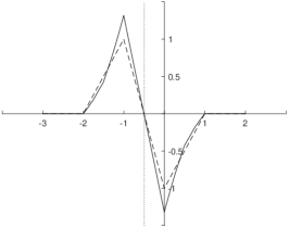
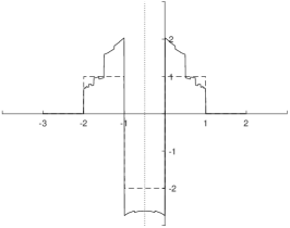
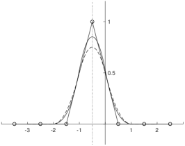
Figure 1: Limit functions of the classical corner-cutting algorithm (dashed line) and the proposed scheme (real line), and their first- and second-order derivatives.

6 Numerical examples

In this section, we present some numerical examples to demonstrate the performance of the NUCC scheme. The first example verifies that the proposed NUCC scheme is C1superscript𝐶1C^{1}. It supports the theoretical result in Section 4.

Example 6.1.

(Smoothness) In this example, we put the initial data 𝐟0superscript𝐟0{\mathbf{f}}^{0} as the Kronecker delta sequence, i.e., 𝐟0={𝐟j0:=δj,0:j}superscript𝐟0conditional-setassignsubscriptsuperscript𝐟0𝑗subscript𝛿𝑗0𝑗{\mathbf{f}}^{0}=\{{\mathbf{f}}^{0}_{j}:=\delta_{j,0}:j\in\mathbb{Z}\} where δj,0subscript𝛿𝑗0\delta_{j,0} equals zero, if j0𝑗0j\neq 0, and one otherwise. In order to get the limit function, we recursively apply the refinement rule {Sk}subscript𝑆𝑘\{S_{k}\} to 𝐟0superscript𝐟0{\mathbf{f}}^{0} using the mask given in (6). In this experiment, we set ϵitalic-ϵ\epsilon in the shape parameter γjsubscript𝛾𝑗\gamma_{j} as |ϵ|=1italic-ϵ1|\epsilon|=1. We compare the limit function with the one generated by the classical corner-cutting algorithm. Figure 1 depicts the two limit functions, and their first- and second-order derivatives.

Table 1: Comparison of the approximation order to the function defined in (34).
Density of initial data Max. Error Approximation Order
Exp. B-spline Proposed Exp. B-spline Proposed
1 8.6789E-02 5.0305E-02
21superscript212^{-1} 2.3629E-02 6.2276E-03 1.9 3.0
22superscript222^{-2} 6.1175E-03 6.2632E-04 1.9 3.3
23superscript232^{-3} 1.5701E-03 7.5863E-05 2.0 3.0
24superscript242^{-4} 3.9306E-04 9.2633E-06 2.0 3.0
25superscript252^{-5} 9.8297E-05 1.1537E-06 2.0 3.0
26superscript262^{-6} 2.4576E-05 1.4397E-07 2.0 3.0
27superscript272^{-7} 6.1442E-06 1.7986E-08 2.0 3.0
28superscript282^{-8} 1.5360E-06 2.2479E-09 2.0 3.0
29superscript292^{-9} 3.8394E-07 2.8126E-10 2.0 3.0
Refer to caption
Refer to caption
Refer to caption
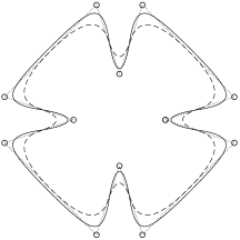
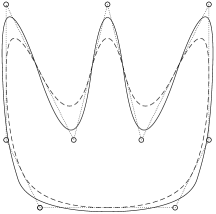
Figure 2: Curve-fitting results: classical corner-cutting method (dashed line) and the new algorithm with |ϵ|=1italic-ϵ1|\epsilon|=1 (real line).

The following example treats the approximation order of the NUCC scheme discussed in Section 5,

Example 6.2.

(Approximation order) This example tests the numerical approximation order of the NUCC scheme for the (scaled one-dimensional Franke) function

f(t):=34e(98t2)2/4+34e(98t+1)2/49+12e(98t7)2/415e(98t4)2.assign𝑓𝑡34superscript𝑒superscript98𝑡22434superscript𝑒superscript98𝑡124912superscript𝑒superscript98𝑡72415superscript𝑒superscript98𝑡42\displaystyle f(t):=\frac{3}{4}e^{-(\frac{9}{8}t-2)^{2}/4}+\frac{3}{4}e^{-(\frac{9}{8}t+1)^{2}/49}+\frac{1}{2}e^{-(\frac{9}{8}t-7)^{2}/4}-\frac{1}{5}e^{-(\frac{9}{8}t-4)^{2}}. (34)

The initial data is sampled from the function f𝑓f with density 2k0superscript2subscript𝑘02^{-k_{0}} for k0=0,,9subscript𝑘009k_{0}=0,\ldots,9. As verified in [27], an exponential B-spline subdivision can provide the approximation order at most two when a suitable normalization factor is taken. Thus, we employ the normalized exponential B-spline scheme of degree 222 reproducing two exponential polynomials {exp(γ),exp(γ)}\{\exp(\gamma\cdot),\exp(-\gamma\cdot)\} with γ=1/2𝛾12\gamma=1/2. The corresponding subdivision masks are given by

𝐚2[k]=sinh(2k3)sinh(2k1),𝐚1[k]=sinh(32k3)sinh(2k1),𝐚0[k]=𝐚1[k],𝐚1[k]=𝐚2[k].formulae-sequencesubscriptsuperscript𝐚delimited-[]𝑘2superscript2𝑘3superscript2𝑘1formulae-sequencesubscriptsuperscript𝐚delimited-[]𝑘13superscript2𝑘3superscript2𝑘1formulae-sequencesubscriptsuperscript𝐚delimited-[]𝑘0subscriptsuperscript𝐚delimited-[]𝑘1subscriptsuperscript𝐚delimited-[]𝑘1subscriptsuperscript𝐚delimited-[]𝑘2\displaystyle{\mathbf{a}}^{[k]}_{-2}=\frac{\sinh(2^{-k-3})}{\sinh(2^{-k-1})},\quad{\mathbf{a}}^{[k]}_{-1}=\frac{\sinh(3\cdot 2^{-k-3})}{\sinh(2^{-k-1})},\quad{\mathbf{a}}^{[k]}_{0}={\mathbf{a}}^{[k]}_{-1},\quad{\mathbf{a}}^{[k]}_{1}={\mathbf{a}}^{[k]}_{-2}.

Table 1 displays the experimental results. As one can see in Table 1, the NUCC scheme achieves the third-order accuracy while the exponential B-spline scheme attains the second order accuracy.

Example 6.3.

(Curve fitting) In this example, we compare the curve-fitting performance of the classical corner-cutting method and the NUCC algorithm. Figure 2 shows the resulting curves generated from several initial data. For this experiment, we used |ϵ|=1italic-ϵ1|\epsilon|=1. The limit curves of the proposed algorithm better follow the sharp corners than those of the classical scheme.

Acknowledgements J. Yoon was supported in part by the National Research Foundation of Korea under grant NRF-2020R1A2C1A01005894.

References

  • [1] C. Beccari, G. Casciola, L. Romani, A non-stationary uniform tension controlled interpolating 4-point scheme reproducing conics, Comput. Aided Geom. Design, 24 (2007) 1–9.
  • [2] C. de Boor, Cutting corners always works, Comput. Aided Geom. Design, 4 (1987) 125–131.
  • [3] A. Cavaretta, W. Dahmen, C. A. Micchelli, Stationary Subdivision, Mem. Amer. Math. Soc. 93(453) (1991) 1-186.
  • [4] E. Catmull, J. Clark, Recursively generated B-spline surfaces on arbitrary topological meshes, Comput. Aided Design 10 (1978) 350-355.
  • [5] G. M. Chaikin, An algorithm for high speed curve generation, Comput. Vis. Graph. Image Process. 3 (1974) 346–349.
  • [6] M. Charina, C. Conti, Polynomial reproduction of multivariate scalar subdivision schemes, J. Comput. Appl. Math., 240 (2013) 51–61.
  • [7] M. Charina, C. Conti, L. Romani, Reproduction of exponential polynomials by multivariate non-stationary subdivision schemes with a general dilation matrix, Numer. Math., 127(2) (2014) 223–254.
  • [8] E. Cohen, T. Lyche, R. Riesenfeld, Discrete B-splines and subdivision techniques in Computer-Aided Geometric Design and Computer Graphics, Comput. Graph. and Image Process 14 (1980) 87-111.
  • [9] C. Conti, N. Dyn, Convergence and smoothness of tensor-product of two non-uniform linear subdivision schemes, Comput. Aided Geom. Design 66 (2018) 16-18.
  • [10] C. Conti, K. Hormann, Polynomial reproduction for univariate subdivision schemes of any arity, J. Approx. Theory, 163 (2011) 413–437.
  • [11] C. Conti, L. Gemignani, L. Romani, From approximating to interpolatory non-stationary subdivision schemes with the same generation properties, Adv. Comput. Math., 35(2-4) (2011) 217–241.
  • [12] C. Conti, L. Gemignani, L. Romani, Exponential pseudo-splines: Looking beyond exponential B-splines, J. Math. Anal. Appl. 439(1) (2016) 32–56.
  • [13] C. Conti, L. Romani, Algebraic conditions on non-stationary subdivision symbols for exponential polynomial reproduction, J. Comput. Appl. Math. 236 (2011) 543–556.
  • [14] G. Deslauriers, S. Dubuc, Symmetric iterative interpolation, Constr. Approx. 5 (1989) 49–68.
  • [15] R. Donat, D. F. Yáñez, A nonlinear Chaikin-based binary subdivision scheme, J. Comput. Appl. Math. 349 (2019) 379-389.
  • [16] D. Doo, M. Sabin, Behaviour of recursive division surfaces near extraordinary points, Comput. Aided Des. 10(6) (1978) 356-360.
  • [17] N. Dyn, Subdivision Schemes in Computer-Aided Geometric Design, Advances in Numerical Analysis Vol. II: Wavelets, Subdivision Algorithms and Radial Basis Functions (W.A. Light ed.), Oxford University Press (1992), 36-104.
  • [18] N. Dyn, K. Hormann, M.A. Sabin, Z. Shen, Polynomial reproduction by symmetric subdivision schemes, J. Approx. Theory, 155 (2008) 28–42.
  • [19] N. Dyn, D. Levin, The subdivision experience, In Laurent, P., LeMéhauté, A. and Schumaker, L. (eds.): Curves and surfaces II, Wellesley, MA: A. K. Peters, 1991.
  • [20] N. Dyn, D. Levin, Analysis of asymptotically equivalent binary subdivision schemes, J. Math. Anal. Appl. 193 (1995) 594-621.
  • [21] N. Dyn, D. Levin, Subdivision schemes in geometric modelling, Acta Numerica 11, (2002), 73-144.
  • [22] N. Dyn, D. Levin, A. Luzzatto, Exponential reproducing subdivision schemes, Found. Comput. Math., 3 (2003) 187–206.
  • [23] N. Dyn, D. Levin, J. Yoon, A new method for the analysis of univariate nonuniform subdivision schemes, Constr. Approx. 40 (2014) 173-188.
  • [24] M.-e Fang, W. Ma, G. Wang, A generalized curve subdivision scheme of arbitrary order with a tension parameter, Comput. Aided Geom. Design, 27 (2010) 720-733.
  • [25] J. A. Gregory, R. Qu, Nonuniform corner cutting, Comput. Aided Geom. Design, 13 (1996) 763-772.
  • [26] M. K. Jena, P. Shunmugaraj, P. C. Das, A non-stationary subdivision scheme for curve interpolation Anziam J. 44(E) (2003) 216–235.
  • [27] B. Jeong, H. O. Kim, Y. J. Lee, J. Yoon, Exponential polynomial reproducing property of non-stationary symmetric subdivision schemes and normalized exponential B-splines, Adv. Comput. Math. 38 (2013) 647-666.
  • [28] B. Jeong, Y.J. Lee, J. Yoon, A family of non-stationary subdivision schemes reproducing exponential polynomials, J. Math. Anal. Appl. 402(1) (2013) 207–219.
  • [29] I. Khalidov and M. Unser From differential equations to the construction of wavelet-like bases, IEEE Tran. Sig. Proc., 54 (2005), 1256-1267.
  • [30] A. Levin, Polynomial generation and quasi-interpolation in stationary non-uniform subdivision, Comput. Aided Geom. Design, 20(1) (2003) 41–60.
  • [31] A. Ron, Exponential box splines, Constr. Approx., 4 (1988) 357-378.
  • [32] L. Romani, A Chaikin-based variant of Lane–Riesenfeld algorithm and its non-tensor product extension, Comput. Aided Geom. Design, 32 (2015) 22-49.
  • [33] Y. Tian, M. Pan, Corner-cutting subdivision surfaces of general degrees with parameters, J. Comput. Math. 38(5) (2020) 710-725.
  • [34] M. Unser and T. Blu Cardinal Exponential Splines : Part I -Theory and Filtering Algorithms, IEEE Tran. Sig. Proc., 53 (2005), 1425-1438.
  • [35] C. Vonesch, T. Blu and M. Unser Generalized Daubechies Wavelet Families, IEEE Tran. Sig. Proc., 55 (2007), 4415-4429.