Subgroup-based Rank-1 Lattice Quasi-Monte Carlo

Abstract

Quasi-Monte Carlo (QMC) is an essential tool for integral approximation, Bayesian inference, and sampling for simulation in science, etc. In the QMC area, the rank-1 lattice is important due to its simple operation, and nice properties for point set construction. However, the construction of the generating vector of the rank-1 lattice is usually time-consuming because of an exhaustive computer search. To address this issue, we propose a simple closed-form rank-1 lattice construction method based on group theory. Our method reduces the number of distinct pairwise distance values to generate a more regular lattice. We theoretically prove a lower and an upper bound of the minimum pairwise distance of any non-degenerate rank-1 lattice. Empirically, our methods can generate a near-optimal rank-1 lattice compared with the Korobov exhaustive search regarding the $l_{1}$-norm and $l_{2}$-norm minimum distance. Moreover, experimental results show that our method achieves superior approximation performance on benchmark integration test problems and kernel approximation problems.

1 Introduction

Integral operation is critical in a large amount of interesting machine learning applications, e.g. kernel approximation with random feature maps [29], variational inference in Bayesian learning [3], generative modeling and variational autoencoders [15]. Directly calculating an integral is usually infeasible in these real applications. Instead, researchers usually try to find an approximation for the integral. A simple and conventional approximation is Monte Carlo (MC) sampling, in which the integral is approximated by calculating the average of the i.i.d. sampled integrand values. Monte Carlo (MC) methods [12] are widely studied with many techniques to reduce the approximation error, which includes importance sampling and variance reduction techniques and more [1].

To further reduce the approximation error, Quasi-Monte Carlo (QMC) methods utilize a low discrepancy point set instead of the i.i.d. sampled point set used in the standard Monte Carlo method. There are two main research lines in the area of QMC [8, 25], i.e., the digital nets/sequences and lattice rules. The Halton sequence and the Sobol sequence are the widely used representatives of digital sequences [8]. Compared with digital nets/sequences, the points set of lattice rules preserve the properties of lattice. The points partition the space into small repeating cells. Among previous research on the lattice rules, Korobov introduced integration lattice rules in [16] for an integral approximation of the periodic integrands. [33] proves that there also exist good lattice rules for non-periodic integrands. According to general lattice rules, a point set is usually constructed by enumerating the integer vectors and multiplying them with an invertible generator matrix. A general lattice rule has to check each constructed point to see whether it is inside a unit cube and discard it if it is not. The process is repeated until we reach the desired number of points. This construction process is inefficient since the checking step is required for every point. Note that rescaling the unchecked points by the maximum norm of all the points may lead to non-uniform points set in the cube.

An interesting special case of the lattice rules is the rank-1 lattice, which only requires one generating vector to construct the whole point set. Given the generating vector, rank-1 lattices can be obtained by a very simple construction form. It is thus much more efficient to construct the point set with the simple construction form. Compared with the general lattice rule, the construction form of the rank-1 lattice has already guaranteed the constructed point to be inside the unit cube, therefore, no further checks are required. We refer to [8] and [25] for a more detailed survey of QMC and rank-1 lattice.

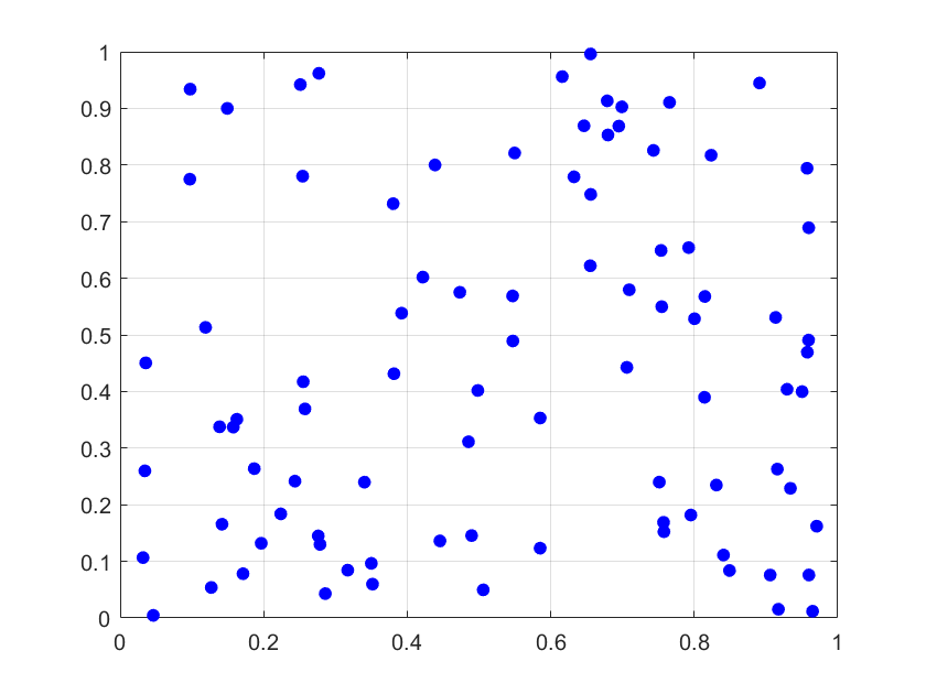
(a) i.i.d. Monte Carlo sampling

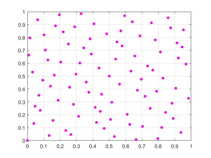
(b) Sobol sequence

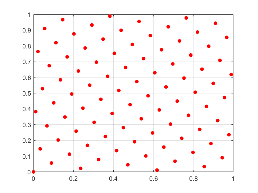
(c) Our subgroup rank-1 lattice

Figure 1: The 89 points constructed by i.i.d. Monte Carlo sampling, Sobol sequence and our subgroup rank-1 lattice on $[0,1]^{2}$.

Although the rank-1 lattice can derive a simple construction form, obtaining the generating vector remains difficult. Most methods [17, 26, 9, 21, 20, 18, 27] in the literature rely on an exhaustive computer search by optimizing some criteria to find a good generating vector. Korobov [17] suggests searching the generating vector in a form of $[1,\alpha,\alpha^{2},\cdots,\alpha^{d-1}]$ with $\alpha\in\{1,\cdots,n-1\}$, where $d$ is the dimension and $n$ is the number of points, such that the greatest common divisor of $\alpha$ and $n$ equals to 1. Sloan et al. study the component-by-component construction for the lattice rules [32]. It is a greedy search that is faster than an exhaustive search. Nuyens et al. [26] propose a fast algorithm to construct the generating vector using a component-by-component search method. Although the exhaustive checking steps are avoided compared with general lattice rules, the rank-1 lattice still requires a brute-force search for the generating vector, which is still very time-consuming, especially when the dimension and the number of points are large.

To address this issue, we propose a closed-form rank-1 lattice rule that directly computes a generating vector without any search process. To generate a more evenly spaced lattice, we propose to reduce the number of distinct pairwise distance in the lattice point set to make the lattice more regular w.r.t. the minimum toroidal distance [11]. Larger minimum toroidal distance means more regular. Based on group theory, we derive that if the generating vector $\boldsymbol{z}$ satisfies the condition that set $\{\boldsymbol{z},-\boldsymbol{z}\}:=\{z_{1},\cdots,z_{d},-z_{1},\cdots,-z_{d}\}$ is a subgroup of the multiplicative group of integers modulo $n$, where $n$ is the number of points, then the number of distinct pairwise distance can be efficiently reduced. We construct the generating vector by ensuring this condition. With the proposed subgroup-based rank-1 lattice, we can construct a more evenly spaced lattice. An illustration of the generated lattice is shown in Figure 1.

Our contributions are summarized as follows:

• We propose a simple and efficient closed-form method for rank-1 lattice construction, which does not require the time-consuming exhaustive computer search that previous rank-1 lattice algorithms rely on. A side product is a closed-form method to generate QMC points set on sphere $\mathbb{S}^{d-1}$ with bounded mutual coherence, which is presented in Appendix.

• We generate a more regular lattice by reducing the number of distinct pairwise distances. We prove a lower and an upper bound for the minimum $l_{1}$-norm-based and $l_{2}$-norm-based toroidal distance of the rank-1 lattice. Theoretically, our constructed lattice is the optimal rank-1 lattice for maximizing the minimum toroidal distance when the number of points $n$ is a prime number and $n=2d+1$.

• Empirically, the proposed method generates near-optimal rank-1 lattice compared with the Korobov search method in maximizing the minimum of the $l_{1}$-norm-based and $l_{2}$-norm-based toroidal distance.

• Our method obtains better approximation accuracy on benchmark test problems and kernel approximation problem.

2 Background

We first give the definition and the properties of lattices in Section 2.1. Then we introduce the minimum distance criterion for lattice construction in Section 2.2.

2.1 The Lattice

A $d$-dimensional lattice $\Lambda$ is a set of points that contains no limit points and satisfies [22]

$$\forall\boldsymbol{x},\boldsymbol{x}^{\prime}\in\Lambda\Rightarrow\boldsymbol{x}+\boldsymbol{x}^{\prime}\in\Lambda\;\text{and}\;\boldsymbol{x}-\boldsymbol{x}^{\prime}\in\Lambda.$$ (1)

A widely known lattice is the unit lattice $\mathbb{Z}^{d}$ whose components are all integers. A general lattice is constructed by a generator matrix. Given a generator matrix $\boldsymbol{B}\in\mathbb{R}^{d\times d}$, a $d$-dimensional lattice $\Lambda$ can be constructed as

$$\Lambda=\{\boldsymbol{By}\big{|}\;\boldsymbol{y}\in\mathbb{Z}^{d}\}.$$ (2)

A generator matrix is not unique to a lattice $\Lambda$, namely, a lattice $\Lambda$ can be obtained from a different generator matrices.

A lattice point set for integration is constructed as $\Lambda\cap[0,1)^{d}$. This step may require an additional search (or check) for all the points inside the unit cube.

A rank-1 lattice is a special case of the general lattice, which has a simple operation for point set construction instead of directly using Eq.(2). A rank-1 lattice point set can be constructed as

$$\boldsymbol{x}_{i}:=\left\langle\frac{i\boldsymbol{z}}{n}\right\rangle,i\in\{0,1,\cdots,n-1\},$$ (3)

where $\boldsymbol{z}\in\mathbb{Z}^{d}$ is the so-called generating vector, and the big $\langle\cdot\rangle$ denotes the operation of taking the fractional part of the input number elementwise. Compared with the general lattice rule, the construction form of the rank-1 lattice already ensures the constructed points to be inside the unit cube without the need for any further checks.

Given a rank-1 lattice set $X$ in the unit cube, we can also construct a randomized point set. Sample a random variable $\boldsymbol{\Delta}\sim Uniform[0,1]^{d}$, we can construct a point set $\widetilde{X}$ by random shift as [8]

$$\widetilde{X}=\left\langle X+\boldsymbol{\Delta}\right\rangle.$$ (4)

2.2 The separating distance of a lattice

Several criteria have been studied in the literature for good lattice construction through computer search. Worst case error is one of the most widely used criteria for functions in a reproducing kernel Hilbert space (RKHS) [8]. However, this criterion requires the prior knowledge of functions and the assumption of the RKHS. Without assumptions of the functions, it is reasonable to construct a good lattice by designing an evenly spaced point set. Minimizing the covering radius is a good way for evenly spaced point set construction.

As minimizing the covering radius of the lattice is equivalent to maximizing the packing radius [7], we can construct the point set through maximizing the packing radius (separating distance) of the lattice. Define the covering radius and packing radius of a set of points $X=\{x_{1},...,x_{N}\}$ as Eq.(5) and Eq.(6), respectively:

$$h_{X}=\sup_{x\in\mathcal{X}}{\min_{x_{k}\in X}}\|x-x_{k}\|,$$ (5)

$$\rho_{X}=\frac{1}{2}\min_{\begin{subarray}{c}x_{i},x_{j}\in X,\\ x_{i}\neq x_{j}\end{subarray}}\|x_{i}-x_{j}\|.$$ (6)

The $l_{p}$-norm-based toroidal distance [11] between two lattice points ${\bf{x}}\in[0,1]^{d}$ and ${\bf{x}^{\prime}}\in[0,1]^{d}$ can be defined as:

$$\|{\bf{x}}-{\bf{x}^{\prime}}\|_{T_{p}}:=\!\!\left(\sum_{i=1}^{d}(\min(|x_{i}-x^{\prime}_{i}|,1-|x_{i}-x^{\prime}_{i}|))^{p}\right)^{\frac{1}{p}}$$ (7)

Because the difference (subtraction) between two lattice points is still a lattice point, and a rank-1 lattice has a period 1, the packing radius $\rho_{X}$ of a rank-1 lattice can be calculated as

$$\rho_{X}=\min_{{\bf{x}}\in{X\setminus{\bf{0}}}}\frac{1}{2}\|{\bf{x}}\|_{T_{2}},$$ (8)

where $\|{\bf{x}}\|_{T_{2}}$ denotes the $l_{2}$-norm-based toroidal distance between $\bf{x}$ and $\bf{0}$, symbol $X\setminus{\bf{0}}$ denotes the set $X$ excludes the point $\boldsymbol{0}$. This formulation calculates the packing radius with a time complexity of $\mathcal{O}(Nd)$ rather than $\mathcal{O}(N^{2}d)$ in pairwise comparison. However, the computation of the packing radius is not easily accelerated by fast Fourier transform due to the minimum operation in Eq.(8).

3 Subgroup-based Rank-1 Lattice

In this section, we derive our construction of a rank-1 lattice based on the subgroup theory. Then we analyze the properties of our method. We provide detailed proofs in the supplement.

3.1 Construction of the Generating Vector

From the definition of rank-1 lattice, we know the packing radius of rank-1 lattice with $n$ points can be reformulated as

$$\rho_{X}=\min_{i\in\{1,\cdots,n-1\}}\frac{1}{2}\|{\bf{x}}_{i}\|_{T_{2}},$$ (9)

where

$$\boldsymbol{x}_{i}:=\frac{i\boldsymbol{z}\;\text{mod}\;n}{n},i\in\{1,...,n-1\}.$$ (10)

Then, we have

$$\rho_{X} =\min_{i\in\{1,\cdots,n-1\}}\frac{1}{2}\left\|\text{min}\left(\frac{i\boldsymbol{z}\;\text{mod}\;n}{n},\frac{n-i\boldsymbol{z}\;\text{mod}\;n}{n}\right)\right\|_{2}$$

$$=\min_{i\in\{1,\cdots,n-1\}}\frac{1}{2}\left\|\text{min}\left(\frac{i\boldsymbol{z}\;\text{mod}\;n}{n},\frac{(-i\boldsymbol{z})\;\text{mod}\;n}{n}\right)\right\|_{2},$$ (11)

where $\text{min}(\cdot,\cdot)$ denotes the elementwise min operation between two inputs.

Suppose $n$ is a prime number, from number theory, we know that for a primitive root $g$, the residue of $\{g^{0},g^{1},\cdots,g^{n-2}\}$ modulo $n$ forms a cyclic group under multiplication, and $g^{n-1}\equiv 1\;\text{mod}\;n$. Since $(g^{\frac{n-1}{2}})^{2}=g^{n-1}\equiv 1\;\text{mod}\;n$, we know that $g^{\frac{n-1}{2}}\equiv-1\;\text{mod}\;n$.

Because of the one-to-one correspondence between the residue of $\{g^{0},g^{1},\cdots,g^{n-2}\}$ modulo $n$ and the set $\{1,2,\cdots,n-1\}$, we can construct the generating vector as

$$\boldsymbol{z}=[g^{m_{1}},g^{m_{2}},\cdots,g^{m_{d}}]\;\text{mod}\;n$$ (12)

without loss of generality, where $m_{1},\cdots,m_{d}$ are integer components to be designed. Denote $\boldsymbol{\bar{z}}=[g^{\frac{n-1}{2}+m_{1}},g^{\frac{n-1}{2}+m_{2}},\cdots,g^{\frac{n-1}{2}+m_{d}}]\;\text{mod}\;n$, maximizing the separating distance $\rho_{X}$ is equivalent to maximizing

$$J\!=\!\min_{k\in\{0,\cdots,n-2\}}\left\|\text{min}(g^{k}\boldsymbol{z}\;\text{mod}\;n,g^{k}\boldsymbol{\bar{z}}\;\text{mod}\;n)\right\|_{2}.$$ (13)

Suppose $2d$ divides $n-1$, i.e., $2d|(n-1)$, by setting $m_{i}=g^{\frac{(i-1)(n-1)}{2d}}$ for $i\in\{1,\cdots,d\}$, we know that $H=\{g^{m_{1}},g^{m_{2}},\cdots,g^{m_{d}},g^{\frac{n-1}{2}+m_{1}},g^{\frac{n-1}{2}+m_{2}},\cdots,g^{\frac{n-1}{2}+m_{d}}\}$ is equivalent to setting $\{g^{0},g^{\frac{n-1}{2d}},\cdots,g^{\frac{(2d-1)(n-1)}{2d}}\}$ mod $n$ , and it forms a subgroup of the group $\{g^{0},g^{1},\cdots,g^{n-2}\}$ mod $n$. From Lagrange’s theorem in group theory [10], we know that the cosets of the subgroup $H$ partition the entire group $\{g^{0},g^{1},\cdots,g^{n-2}\}$ into equal-size, non-overlapping sets, and the number of cosets of $H$ is $\frac{n-1}{2d}$. Thus, we know that distance $\text{min}(g^{k}\boldsymbol{z}\;\text{mod}\;n,g^{k}\boldsymbol{\bar{z}}\;\text{mod}\;n)$ for $k\in\{0,\cdots,n-2\}$ has $\frac{n-1}{2d}$ different values, and there are the same numbers of items for each value.

Thus, we can construct the generating vector as

$$\boldsymbol{z}=[g^{0},g^{\frac{n-1}{2d}},g^{\frac{2(n-1)}{2d}},\cdots,g^{\frac{(d-1)(n-1)}{2d}}]\;\text{mod}\;n.$$ (14)

In this way, the constructed rank-1 lattice is more regular as it has few different distinct pairwise distance values, and for each distance, the same number of items obtain this value. Usually, the constructed regular lattice is more evenly spaced, and it has a large minimum pairwise distance. We confirm this empirically through extensive experiments in Section 5.

We summarize our construction method and the properties of the constructed rank-1 lattice in Theorem 1.

Theorem 1.

Suppose $n$ is a prime number and $2d|(n-1)$. Let $g$ be a primitive root of $n$. Let $\boldsymbol{z}=[g^{0},g^{\frac{n-1}{2d}},g^{\frac{2(n-1)}{2d}},\cdots,g^{\frac{(d-1)(n-1)}{2d}}]\;\text{mod}\;n$. Construct a rank-1 lattice $X\!=\!\{\boldsymbol{x}_{0},\cdots,\boldsymbol{x}_{n-1}\}$ with $\boldsymbol{x}_{i}=\frac{i\boldsymbol{z}\;\text{mod}\;n}{n},i\in\{0,...,n-1\}$. Then, there are $\frac{n-1}{2d}$ distinct pairwise toroidal distance values among $X$, and each distance value is taken by the same number of pairs in $X$.

As shown in Theorem 1, our method can construct regular rank-1 lattice through a very simple closed-form construction, which does not require any exhaustive computer search.

3.2 Regular Property of Rank-1 Lattice

We show the regular property of rank-1 lattices in terms of $l_{p}$-norm-based toroidal distance.

Theorem 2.

Suppose $n$ is a prime number and $n\geq 2d+1$. Let $\boldsymbol{z}=[z_{1},z_{2},\cdots,z_{d}]$ with $1\leq z_{k}\leq n-1$. Construct a rank-1 lattice $X=\{\boldsymbol{x}_{0},\cdots,\boldsymbol{x}_{n-1}\}$ with $\boldsymbol{x}_{i}=\frac{i\boldsymbol{z}\;\text{mod}\;n}{n},i\in\{0,...,n-1\}$ and $z_{i}\neq z_{j}$ . Then, the minimum pairwise toroidal distance can be bounded as

$$\frac{d(d+1)}{2n}\leq\min_{i,j\in\{0,\cdots,n-1\},i\neq j}\|{\bf{x}}_{i}-{\bf{x}}_{j}\|_{T_{1}}\leq\frac{(n+1)d}{4n}$$ (15)

$$\frac{\sqrt{6d(d+1)(2d+1)}}{6n}\leq\min_{i,j\in\{0,\cdots,n-1\},i\neq j}\|{\bf{x}}_{i}-{\bf{x}}_{j}\|_{T_{2}}\leq\sqrt{\frac{(n+1)d}{12n}},$$ (16)

where $\|\cdot\|_{T_{1}}$ and $\|\cdot\|_{T_{2}}$ denote the $l_{1}$-norm-based toroidal distance and the $l_{2}$-norm-based toroidal distance, respectively.

Theorem 2 gives the upper and lower bounds of the minimum pairwise distance of any non-degenerate rank-1 lattice. The term ‘non-degenerate’ means that the elements in the generating vector are not equal, i.e., $z_{i}\neq z_{j}$.

We now show that our subgroup-based rank-1 lattice can achieve the optimal minimum pairwise distance when $n=2d+1$ is a prime number.

Corollary 1.

Suppose $n=2d+1$ is a prime number. Let $g$ be a primitive root of $n$. Let $\boldsymbol{z}=[g^{0},g^{\frac{n-1}{2d}},g^{\frac{2(n-1)}{2d}},\cdots,g^{\frac{(d-1)(n-1)}{2d}}]\;\text{mod}\;n$. Construct rank-1 lattice $X=\{\boldsymbol{x}_{0},\cdots,\boldsymbol{x}_{n-1}\}$ with $\boldsymbol{x}_{i}=\frac{i\boldsymbol{z}\;\text{mod}\;n}{n},i\in\{0,...,n-1\}$. Then, the pairwise toroidal distance of the lattice $X$ attains the upper bound.

$$\|{\bf{x}}_{i}-{\bf{x}}_{j}\|_{T_{1}}=\frac{(n+1)d}{4n},\forall i,j\in\{0,\cdots,n-1\},i\neq j,$$ (17)

$$\|{\bf{x}}_{i}-{\bf{x}}_{j}\|_{T_{2}}=\sqrt{\frac{(n+1)d}{12n}},\forall i,j\in\{0,\cdots,n-1\},i\neq j.$$ (18)

Corollary 1 shows a case when our subgroup rank-1 lattice obtains the maximum minimum pairwise toroidal distance. It is useful for expensive black-box functions, where the number of function queries is small. Empirically, we find that our subgroup rank-1 lattice can achieve near-optimal pairwise toroidal distance in many other cases.

4 QMC for Kernel Approximation

Another application of our subgroup rank-1 lattice is kernel approximation. Kernel approximation has been widely studied. A random feature maps is a promising way for kernel approximation. Rahimi et al. study the shift-invariant kernels by Monte Carlo sampling [29]. Yang et al. suggest employing QMC for kernel approximation [35, 2]. Several previous methods work on the construction of structured feature maps for kernel approximation [19, 6, 23]. Apart from other kernel approximation methods designed for specific kernels, QMC can serve as a plug-in for any integral representation of kernels to improve kernel approximation. We include this section to be self-contained.

From Bochner’s Theorem, shift invariant kernels can be expressed as an integral [29]

$$\begin{array}[]{l}{\rm{K}}(\boldsymbol{x},\boldsymbol{y})=\int_{{{\rm{\mathbb{R}}}^{d}}}{{e^{-i{{(\boldsymbol{x}-\boldsymbol{y})}^{\top}}\bf{w}}}p(\bf{w})d\bf{w}},\end{array}$$ (19)

where $i=\sqrt{-1}$, and $p(\bf{w})$ is a probability density. $p({\bf{w}})=p(-{\bf{w}})\geq 0$ ensure the imaginary parts of the integral vanish. Eq.(19) can be rewritten as

$${\rm{K}}(\boldsymbol{x},\boldsymbol{y})=\int_{[0,1]^{d}}{{e^{-i{{(\boldsymbol{x}-\boldsymbol{y})}^{\top}}\Phi^{-1}(\boldsymbol{\epsilon})}}d\boldsymbol{\epsilon}}.$$ (20)

We can approximate the integral Eq.(19) by using our subgroup rank-1 lattice according to the QMC approximation in [35, 34]

$${\rm{K}}(\boldsymbol{x},\boldsymbol{y}) =\int_{[0,1]^{d}}{{e^{-i{{(\boldsymbol{x}-\boldsymbol{y})}^{\top}}\Phi^{-1}(\boldsymbol{\epsilon})}}d\boldsymbol{\epsilon}}\approx\frac{1}{n}\sum_{i=1}^{n}{e^{-i{{(\boldsymbol{x}-\boldsymbol{y})}^{\top}}\Phi^{-1}(\boldsymbol{\epsilon}_{i})}}=\left<\Psi(\boldsymbol{x}),\Psi(\boldsymbol{y})\right>,$$ (21)

where $\Psi(\boldsymbol{x})=\frac{1}{\sqrt{n}}\left[e^{-i\boldsymbol{x}^{\top}\Phi^{-1}(\boldsymbol{\epsilon}_{1})},\cdots,e^{-i\boldsymbol{x}^{\top}\Phi^{-1}(\boldsymbol{\epsilon}_{n})}\right]$ is the feature map of the input $\boldsymbol{x}$.

5 Experiments

In this section, we first evaluate the minimum distance generated by our subgroup rank-1 lattice in section 5.1. We then evaluate the subgroup rank-1 lattice on integral approximation tasks and kernel approximation task in section 5.2 and 5.3, respectively.

Table 1: Minimum $l_{1}$-norm-based toroidal distance of rank-1 lattice constructed by different methods.

d=50		n=101	401	601	701	1201	1301	1601	1801	1901	2801
	SubGroup	12.624	11.419	11.371	11.354	11.029	10.988	10.541	10.501	10.454	10.748
	Hua [13]	10.426	10.421	9.8120	10.267	10.074	9.3982	9.5890	9.5175	8.9868	9.2260
	Korobov [17]	12.624	11.419	11.371	11.354	11.029	10.988	10.665	10.561	10.701	10.748
d=100		401	601	1201	1601	1801	2801	3001	4001	4201	4801
	SubGroup	24.097	23.760	22.887	23.342	22.711	23.324	22.233	22.437	22.573	21.190
	Hua [13]	21.050	21.251	21.205	20.675	19.857	20.683	20.700	19.920	19.967	20.574
	Korobov [17]	24.097	23.760	23.167	23.342	22.893	23.324	22.464	22.437	22.573	22.188
d=200		401	1201	1601	2801	4001	4801	9601	12401	14401	15601
	SubGroup	50.125	48.712	47.500	47.075	47.810	45.957	45.819	46.223	43.982	45.936
	Hua [13]	43.062	43.057	43.052	43.055	43.053	43.055	43.053	42.589	42.558	42.312
	Korobov [17]	50.125	48.712	47.660	47.246	47.810	46.686	46.154	46.223	45.949	45.936
d=500		3001	4001	7001	9001	13001	16001	19001	21001	24001	28001
	SubGroup	121.90	121.99	119.60	118.63	120.23	119.97	116.41	120.56	120.24	113.96
	Hua [13]	108.33	108.33	108.33	108.33	108.33	108.33	108.33	108.33	108.33	108.33
	Korobov [17]	121.90	121.99	120.46	120.16	120.23	119.97	119.41	120.56	120.24	118.86

Table 2: Minimum $l_{2}$-norm-based toroidal distance of rank-1 lattice constructed by different methods.

d=50		n=101	401	601	701	1201	1301	1601	1801	1901	2801
	SubGroup	2.0513	1.9075	1.9469	1.9196	1.8754	1.8019	1.8008	1.8709	1.7844	1.7603
	Hua [13]	1.7862	1.7512	1.7293	1.7049	1.7326	1.6295	1.6659	1.6040	1.5629	1.5990
	Korobov [17]	2.0513	1.9075	1.9469	1.9196	1.8754	1.8390	1.8356	1.8709	1.8171	1.8327
d=100		401	601	1201	1601	1801	2801	3001	4001	4201	4801
	SubGroup	2.8342	2.8143	2.7077	2.7645	2.7514	2.6497	2.6337	2.6410	2.6195	2.5678
	Hua [13]	2.5385	2.5739	2.4965	2.4783	2.4132	2.5019	2.4720	2.4138	2.4537	2.4937
	Korobov [17]	2.8342	2.8143	2.7409	2.7645	2.7514	2.6956	2.6709	2.6562	2.6667	2.6858
d=200		401	1201	1601	2801	4001	4801	9601	12401	14401	15601
	SubGroup	4.0876	3.9717	3.9791	3.8425	3.9276	3.8035	3.7822	3.8687	3.6952	3.8370
	Hua [13]	3.7332	3.7025	3.6902	3.6944	3.7148	3.6936	3.6571	3.5625	3.6259	3.5996
	Korobov [17]	4.0876	3.9717	3.9791	3.9281	3.9276	3.9074	3.8561	3.8687	3.8388	3.8405
d=500		3001	4001	7001	9001	13001	16001	19001	21001	24001	28001
	SubGroup	6.3359	6.3769	6.3141	6.2131	6.2848	6.2535	6.0656	6.2386	6.2673	6.1632
	Hua [13]	5.9216	5.9216	5.9215	5.9215	5.9216	5.9216	5.9215	5.9215	5.8853	5.9038
	Korobov [17]	6.3359	6.3769	6.3146	6.2960	6.2848	6.2549	6.2611	6.2386	6.2673	6.2422

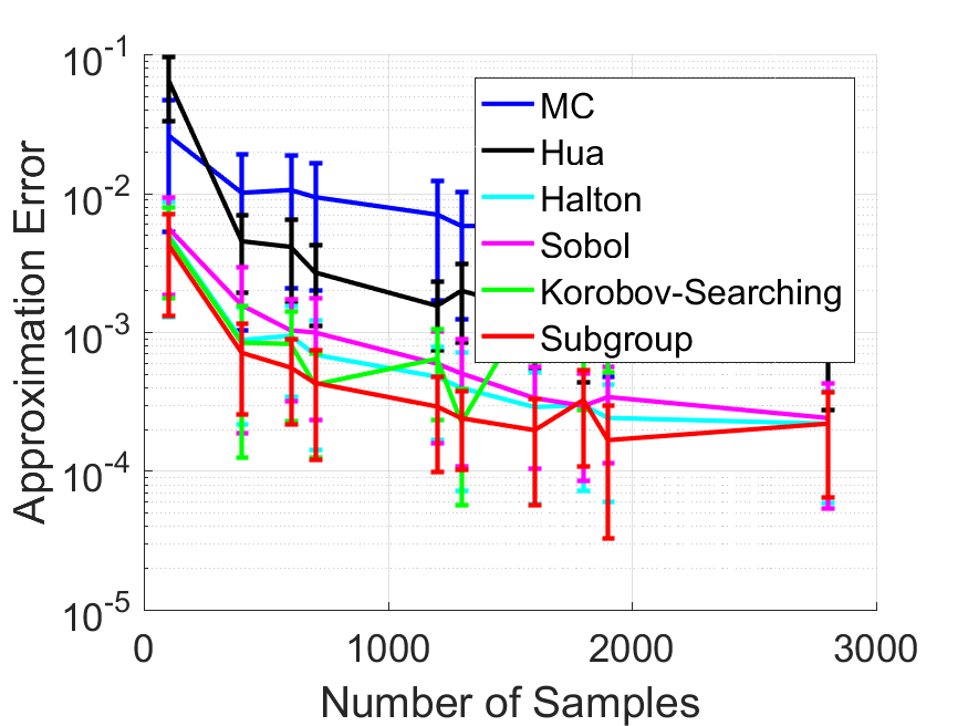
(a) 50-d Integral Approximation

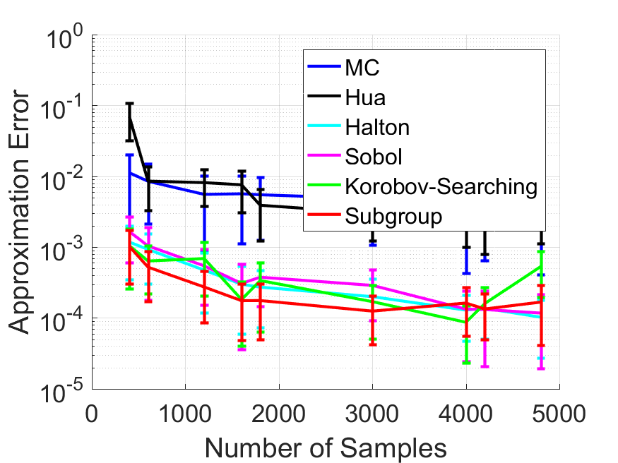
(b) 100-d Integral Approximation

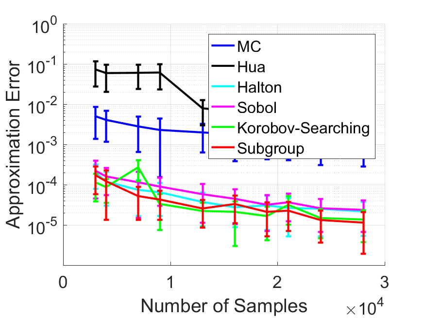
(c) 500-d Integral Approximation

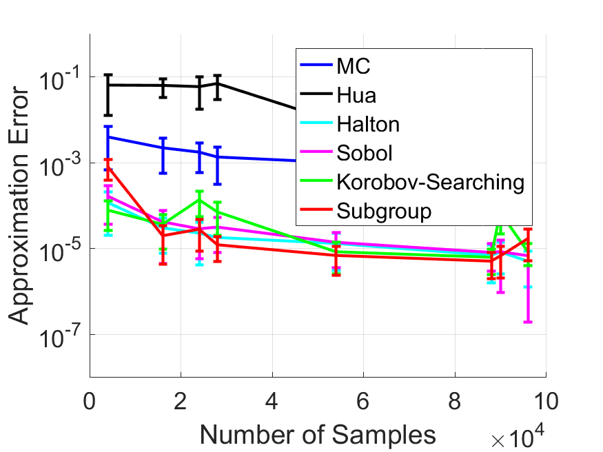
(d) 1000-d Integral Approximation

Figure 2: Mean approximation error over 50 independent runs.error bars are with in $1\times$ std.

5.1 Evaluation of the minimum distance

We evaluate the minimum distance of our subgroup rank-1 lattice by comparing with Hua’s method [13] and the Korobov [17] searching method. We denote ‘SubGroup’ as our subgroup rank-1 lattice, ‘Hua’ as rank-1 lattice constructed by Hua’s method [13], and ‘Korobov’ as rank-1 lattice constructed by exhaustive computer search in Korobov form [17].

We set the dimension $d$ as in $\{50,100,200,500\}$. For each dimension $d$, we set the number of points $n$ as the first ten prime numbers such that $2d$ divides $n\!-\!1$, i.e., $2d\big{|}(n\!-\!1)$. The minimum $l_{1}$-norm-based toroidal distance and the minimum $l_{2}$-norm-based toroidal distance for each dimension are reported in Table 5.1 and Table 2, respectively. The larger the distance, the better.

We can observe that our subgroup rank-1 lattice achieves consistently better (larger) minimum distances than Hua’s method in all the cases. Moreover, we see that subgroup rank-1 lattice obtains, in 20 out of 40 cases, the same $l_{2}$-norm-based toroidal distance and in 24 out of 40 cases the same $l_{1}$-norm-based toroidal distance compared with the exhaustive computer search in Korobov form. The experiments show that our subgroup rank-1 lattice achieves the optimal toroidal distance in exhaustive computer searches in Korobov form in over half of all the cases. Furthermore, the experimental result shows that our subgroup rank-1 lattice obtains a competitive distance compared with the exhaustive Korobov search in the remaining cases. Note that our subgroup rank-1 lattice is a closed-form construction which does not require computer search, making our method more appealing and simple to use.

Time Comparison of Korobov searching and our sub-group rank-1 lattice. The table below shows the time cost (seconds) for lattice construction. The run time for Korobov searching grows fast to hours. Our method can run in less than one second, achieving a $10^{4}\times$ to $10^{5}\times$ speed-up. The speed-up increases when $n$ and $d$ becomes larger.

d=500		n=3001	4001	7001	9001	13001	16001	19001	21001	24001	28001
	SubGroup	0.0185	0.0140	0.0289	0.043	0.0386	0.0320	0.0431	0.0548	0.0562	0.0593
	Korobov	34.668	98.876	152.86	310.13	624.56	933.54	1308.9	1588.5	2058.5	2815.9
d=1000		n=4001	16001	24001	28001	54001	70001	76001	88001	90001	96001
	SubGroup	0.0388	0.0618	0.1041	0.1289	0.2158	0.2923	0.3521	0.4099	0.5352	0.5663
	Korobov	112.18	1849.4	4115.9	5754.6	20257	34842	43457	56798	56644	69323

5.2 Integral approximation

We evaluate our subgroup rank-1 lattice on the integration test problem

$$f(\boldsymbol{x}):=\exp{\Big{(}c\sum_{j=1}^{d}x_{j}j^{-b}\Big{)}}$$ (22)

$$I(f):=\int_{[0,1]^{d}}{f(\boldsymbol{x})d\boldsymbol{x}}=\displaystyle\prod_{j=1}^{d}\frac{\exp(cj^{-b})-1}{cj^{-b}}.$$ (23)

We compare with i.i.d. Monte Carlo, a Hua’s rank-1 lattice [13], Korobov searching rank-1 lattice [16], Halton sequence, and Sobol sequence  [8]. For both Halton sequence and Sobol sequence, we use the scrambling technique suggested in [8]. For all the QMC methods, we use the random shift technique as in Eq.(4).

We fix $b=2$ and $c=1$ in all the experiments. We set dimension $d=100$ and $d=500$, respectively. We set the number of points $n$ as the first ten prime numbers such that $2d$ divides $n\!-\!1$, i.e., $2d\big{|}(n\!-\!1)$.

The mean approximation error ($\frac{|Q(f)-I(f)|}{|I(f)|}$) with error bars over 50 independent runs for each dimension $d$ is presented in Figure 2. We can see that Hua’s method obtains a smaller error than i.i.d Monte Carlo on the 50-d problem, however, it becomes worse than MC on 500-d and 1000-d problems. Moreover, our subgroup rank-1 lattice obtains a consistent smaller error on all the tested problems than Hua and MC. In addition, our subgroup rank-1 lattice achieves a slightly better performance than Halton, Sobol and Korobov searching method.

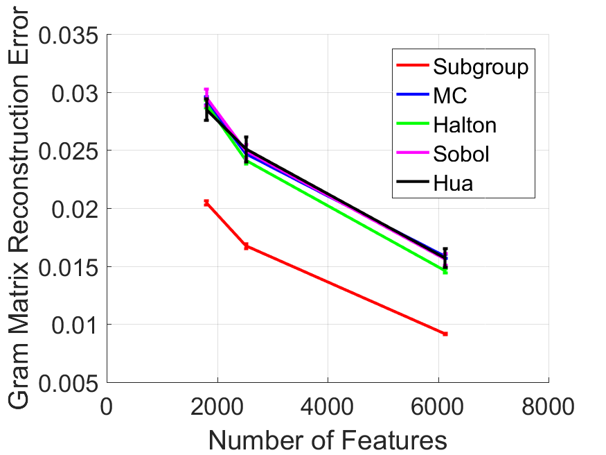
(a) $\frac{{{{\left\|{\widetilde{K}-K}\right\|}_{F}}}}{{{{\left\|K\right\|}_{F}}}}$ for Gaussian Kernel

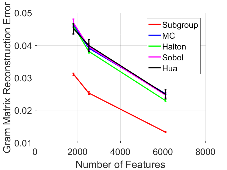
(b) $\frac{{{{\left\|{\widetilde{K}-K}\right\|}_{F}}}}{{{{\left\|K\right\|}_{F}}}}$ for First-order Arc Kernel

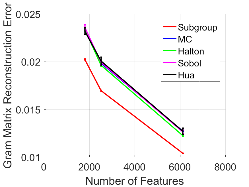
(c) $\frac{{{{\left\|{\widetilde{K}-K}\right\|}_{F}}}}{{{{\left\|K\right\|}_{F}}}}$ for Zero-order Arc Kernel

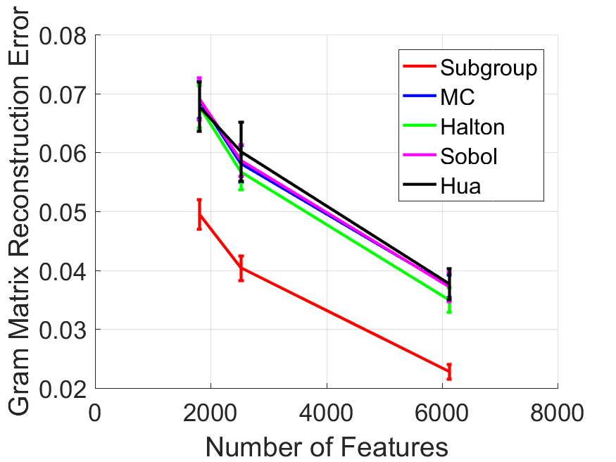
(d) $\frac{{{{\left\|{\widetilde{K}-K}\right\|}_{\infty}}}}{{{{\left\|K\right\|}_{\infty}}}}$ for Gaussian Kernel

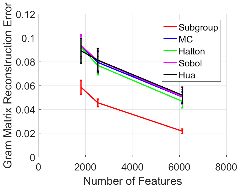
(e) $\frac{{{{\left\|{\widetilde{K}-K}\right\|}_{\infty}}}}{{{{\left\|K\right\|}_{\infty}}}}$ for First-order Arc Kerne

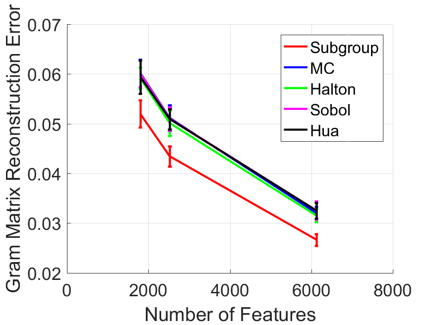
(f) $\frac{{{{\left\|{\widetilde{K}-K}\right\|}_{\infty}}}}{{{{\left\|K\right\|}_{\infty}}}}$ for Zero-order Arc Kernel

Figure 3: Relative Mean and Max Reconstruction Error for Gaussian, Zero-order and First-order Arc-cosine Kernel on DNA dataset. Error bars are within $1\times$ std.

5.3 Kernel approximation

We evaluate the performance of subgroup rank-1 lattice on kernel approximation tasks by comparing with other QMC baseline methods. We test the kernel approximation of the Gaussian kernel, the zeroth-order arc-cosine kernel, and the first-order arc-cosine kernel as in [6].

We compare subgroup rank-1 lattice with a Hua’s rank-1 lattice [13], Halton sequence, Sobol sequence  [8] and standard i.i.d. Monte Carlo sampling. For both the Halton sequence and Sobol sequence, we use the scrambling technique suggested in [8]. For both subgroup rank-1 lattice and Hua’s rank-1 lattice, we use the random shift as in Eq.(4). We evaluate the methods on the DNA [28] and the SIFT1M [14] dataset over 50 independent runs. Each run contains 2000 random samples to construct the Gram matrix. The bandwidth parameter of Gaussian kernel is set to 15 in all the experiments.

The mean Frobenius norm approximation error (${\|{\widetilde{K}\!-\!K}\|}_{F}/{\left\|K\right\|}_{F}$) and maximum norm approximation error (${\|{\widetilde{K}\!-\!K}\|}_{\infty}/{\|K\|}_{\infty}$) with error bars on DNA [28] dataset are plotted in Figure 3. The results on SIFT1M [14] is given in Figure 6 in the supplement. The experimental result shows that subgroup rank-1 lattice consistently obtains a smaller approximation error compared with other baselines.

5.4 Approximation on Graphical Model

For general Boltzmann machines with continuous state in $[0,1]$, the energy function of $\boldsymbol{x}\in[0,1]^{d}$ is defined as $E(\boldsymbol{x})=-(\boldsymbol{x}^{\top}\boldsymbol{W}\boldsymbol{x}+\boldsymbol{b}^{\top}\boldsymbol{x})/d$. The normalization constant is $Z=\int_{[0,1]^{d}}{\exp{(-E(\boldsymbol{x})})d\boldsymbol{x}}$. For inference, the marginal likelihood of observation $\boldsymbol{v}\in\mathbb{R}^{d}$ is $\mathcal{L}(\boldsymbol{v})=\int_{[0,1]^{d}}{\exp{(-f(\boldsymbol{v}))}\exp{(-E(\boldsymbol{h})})/Z\text{d}\boldsymbol{h}}$ with function $f(\boldsymbol{v})=-(\boldsymbol{v}^{\top}\boldsymbol{W}_{v}\boldsymbol{v}+2\boldsymbol{v}^{\top}\boldsymbol{W}_{h}\boldsymbol{h}+\boldsymbol{b}_{v}^{\top}\boldsymbol{v})/d$, where $\boldsymbol{h}\in\mathbb{R}^{d}$ denotes the hidden states.

We evaluate our method on approximation of the normalization constant and inference by comparing with i.i.d. Monte Carlo (MC), slice sampling (SS) and Hamiltonian Monte Carlo (HMC). We generate the elements of $\boldsymbol{W}$, $\boldsymbol{W}_{v}$, $\boldsymbol{W}_{h}$, $\boldsymbol{b}$ and $\boldsymbol{b}_{v}$ by sampling from standard Gaussian $\mathcal{N}(0,1)$. These parameters are fixed and kept the same for all the methods in comparison. For inference, we generate an observation $\boldsymbol{v}\in[0,1]^{d}$ by uniformly sampling and keep it fixed and same for all the methods. For SS and HMC, we use the slicesample function and hmcSampler function in MATLAB, respectively. We use the approximation of i.i.d. MC with $10^{7}$ samples as the pseudo ground-truth. The approximation errors $|\widehat{Z}-Z|/Z$ and $|\widehat{\mathcal{L}}-\mathcal{L}|/\mathcal{L}$ are shown in Fig.4(a)-4(d) and Fig.4(e)-4(h), respectively. our method consistently outperforms MC, HMC and SS on all cases. Moreover, our method is much cheaper than SS and HMC.

(a) 10-d$|\widehat{Z}-Z|/Z$

(b) 50-d $|\widehat{Z}-Z|/Z$

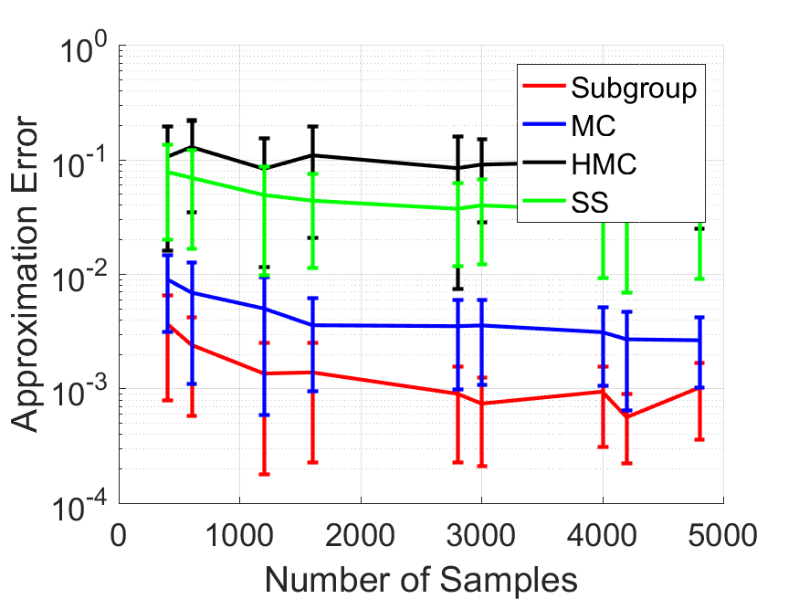
(c) 100-d $|\widehat{Z}-Z|/Z$

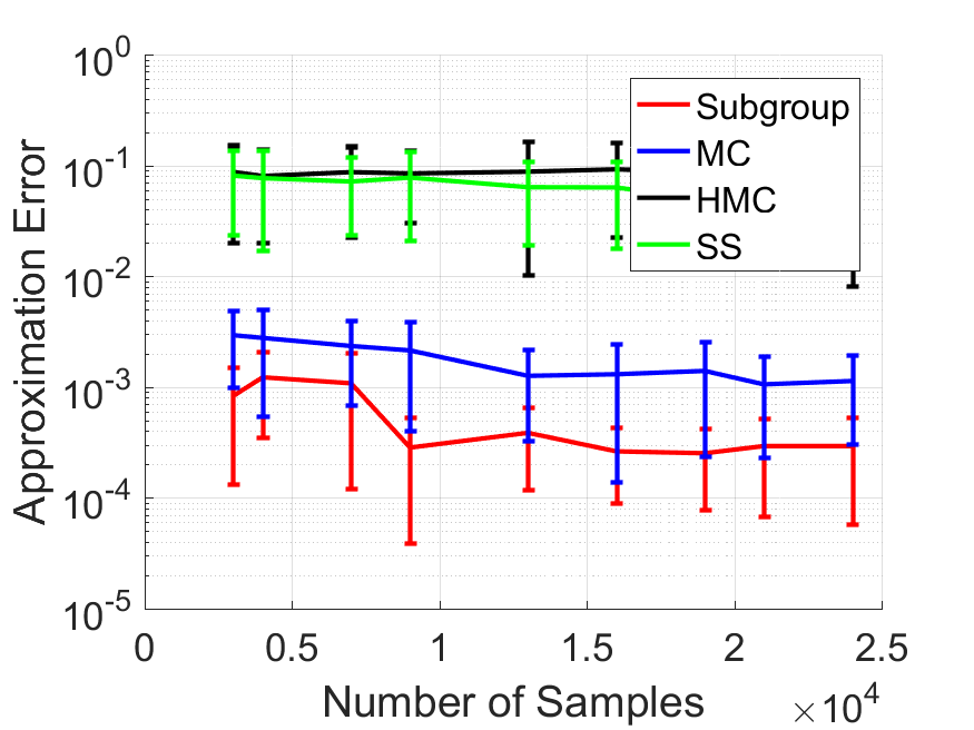
(d) 500-d $|\widehat{Z}-Z|/Z$

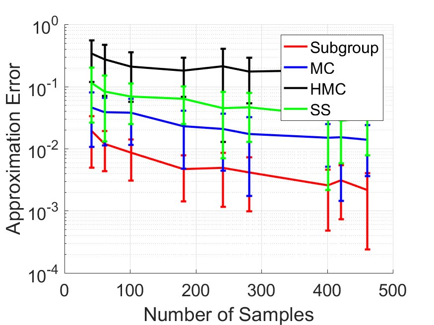
(e) 10-d $|\widehat{\mathcal{L}}-\mathcal{L}|/\mathcal{L}$

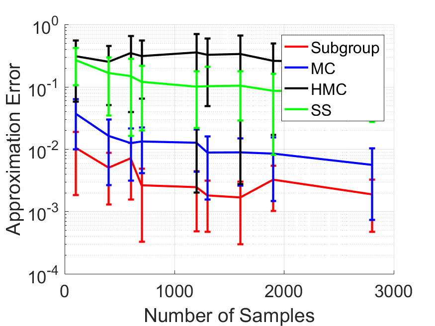
(f) 50-d $|\widehat{\mathcal{L}}-\mathcal{L}|/\mathcal{L}$

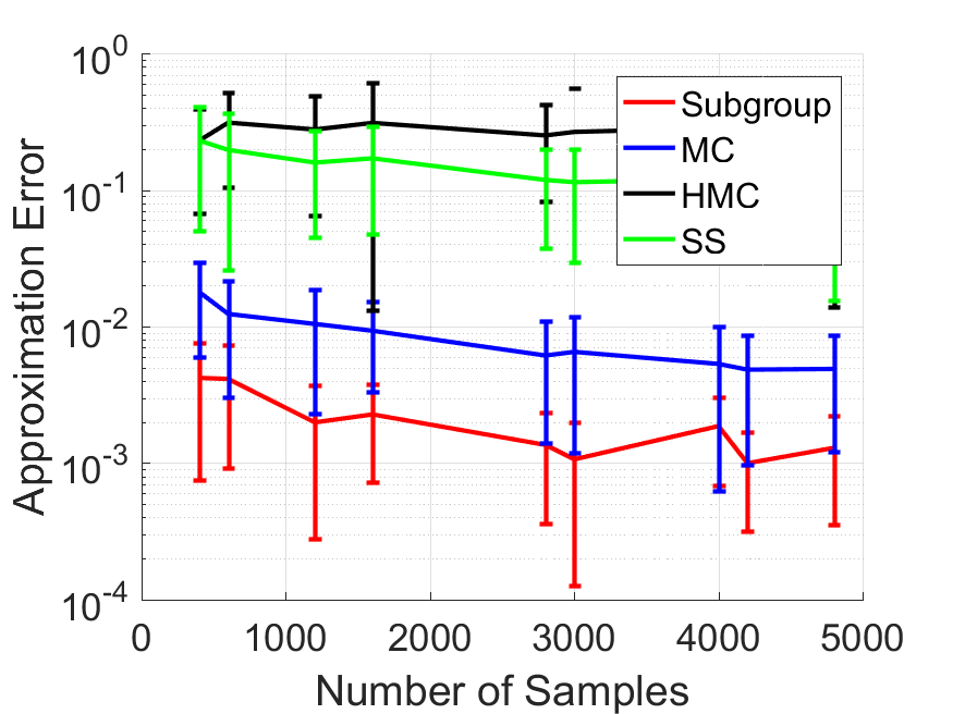
(g) 100-d $|\widehat{\mathcal{L}}-\mathcal{L}|/\mathcal{L}$

(h) 500-d $|\widehat{\mathcal{L}}-\mathcal{L}|/\mathcal{L}$

Figure 4: Mean approximation error over 50 independent runs. Error bars are with in $1\times$ std

Comparison to sequential Monte Carlo. When the positive density region takes a large fraction of the entire domain, our method is very competitive. When it is only inside a small part of a large domain, our method may not be better than sequential adaptive sampling. In this case, it is interesting to take advantage of both lattice and adaptive sampling. E.g., one can employ our subgroup rank-1 lattice as a rough partition of the domain to find high mass regions, then take sequential adaptive sampling on the promising regions with the lattice points as the start points. Also, it is interesting to consider recursively apply our subgroup rank-1 lattice to refine the partition. Moreover, our subgroup-based rank-1 lattice enables black-box evaluation without the need for gradient information. In contrast, several sequential sampling methods, e.g., HMC, need a gradient of density function for sampling.

6 Conclusion

We propose a closed-form method for rank-1 lattice construction, which is simple and efficient without exhaustive computer search. Theoretically, we prove that our subgroup rank-1 lattice has few different pairwise distance values, which is more regular to be evenly spaced. Moreover, we prove a lower and an upper bound for the minimum toroidal distance of a non-degenerate rank-1 lattice. Empirically, our subgroup rank-1 lattice obtains near-optimal minimum toroidal distance compared with Korobov exhaustive search. Moreover, subgroup rank-1 lattice achieves smaller integration approximation error. In addition, we propose a closed-form method to generate QMC points set on sphere $\mathbb{S}^{d-1}$. We proved upper bounds of the mutual coherence of the generated points. Further, we show an example of CycleGAN training in the supplement. Our subgroup rank-1 lattice sampling and QMC on sphere can serve as an alternative for training generative models.

Broader Impact

In this paper, we proposed a closed-form rank-one lattice construction based on group theory for Quasi-Monte Carlo. Our method does not require the time-consuming exhaustive computer search. Our method is a fundamental tool for integral approximation and sampling.

Our method may serve as a potential advance in QMC, which may have an impact on a wide range of applications that rely on integral approximation. It includes kernel approximation with feature map, variational inference in Bayesian learning, generative modeling, and variational autoencoders. This may bring useful applications and be beneficial to society and the community. Since our method focuses more on the theoretical side, the direct negative influences and ethical issues are negligible.

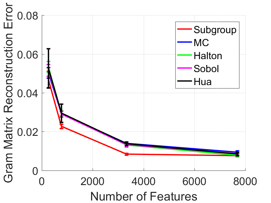
(a) $\frac{{{{\left\|{\widetilde{K}-K}\right\|}_{F}}}}{{{{\left\|K\right\|}_{F}}}}$ for Gaussian Kernel

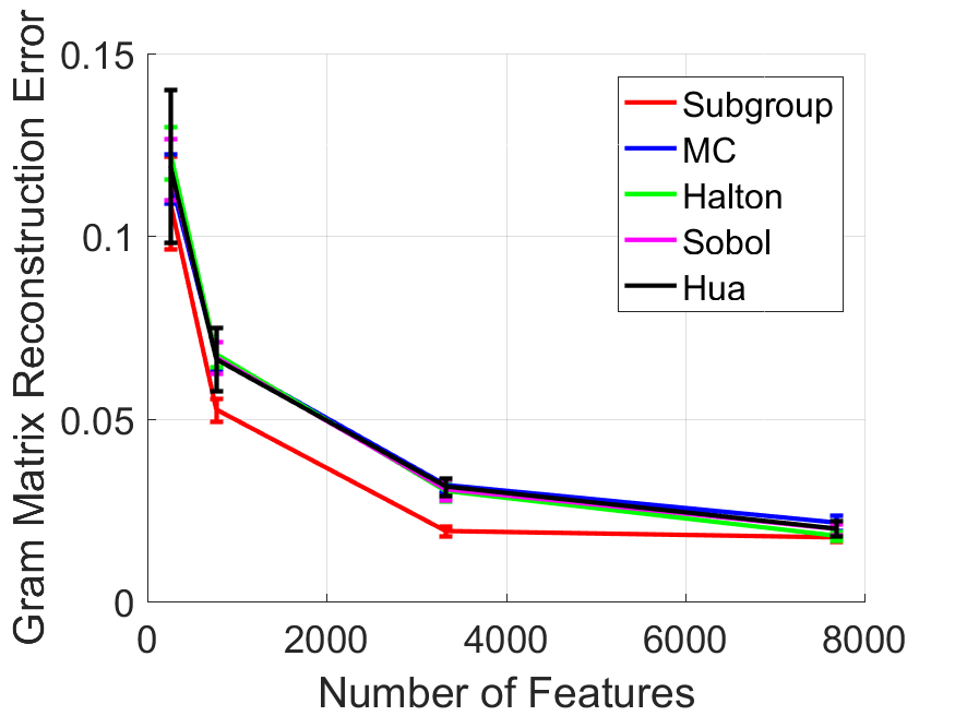
(b) $\frac{{{{\left\|{\widetilde{K}-K}\right\|}_{F}}}}{{{{\left\|K\right\|}_{F}}}}$ for First-order Arc Kernel

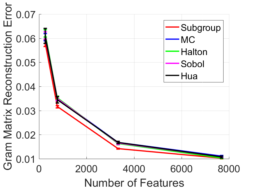
(c) $\frac{{{{\left\|{\widetilde{K}-K}\right\|}_{F}}}}{{{{\left\|K\right\|}_{F}}}}$ for Zero-order Arc Kernel

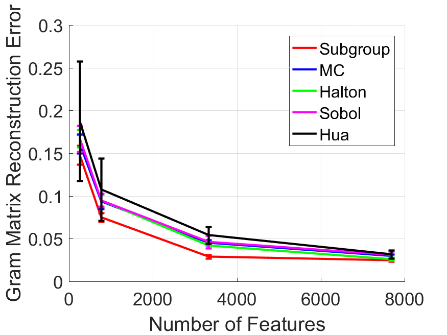
(d) $\frac{{{{\left\|{\widetilde{K}-K}\right\|}_{\infty}}}}{{{{\left\|K\right\|}_{\infty}}}}$ for Gaussian Kernel

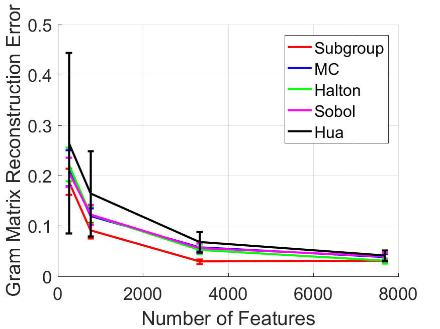
(e) $\frac{{{{\left\|{\widetilde{K}-K}\right\|}_{\infty}}}}{{{{\left\|K\right\|}_{\infty}}}}$ for First-order Arc Kernel

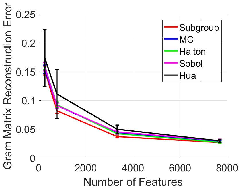
(f) $\frac{{{{\left\|{\widetilde{K}-K}\right\|}_{\infty}}}}{{{{\left\|K\right\|}_{\infty}}}}$ for Zero-order Arc Kernel

Figure 7: Relative Mean and Max Reconstruction Error for Gaussian, Zero-order and First-order Arc-cosine Kernel on SIFT1M dataset.

Organization: In the supplement, we present the detailed proof of the Theorem 1, Theorem 2 and Corollary 1 in section A, section B and section C, respectively. We then present a subgroup-based QMC on sphere $\mathbb{S}^{d-1}$ in Section D. We give the detailed proof of Theorem 3 and Theorem 4 in section E and section F, respectively. We then present QMC for generative CycleGAN in section G and section H. At last, we present the experimental results of kernel approximation on SIFT1M dataset in Figure 7.

Appendix A Proof of Theorem 1

Theorem.

Suppose $n$ is a prime number and $2d|(n-1)$. Let $g$ be a primitive root of $n$. Let $\boldsymbol{z}=[g^{0},g^{\frac{n-1}{2d}},g^{\frac{2(n-1)}{2d}},\cdots,g^{\frac{(d-1)(n-1)}{2d}}]\;\text{mod}\;n$. Construct a rank-1 lattice $X\!=\!\{\boldsymbol{x}_{0},\cdots,\boldsymbol{x}_{n-1}\}$ with $\boldsymbol{x}_{i}=\frac{i\boldsymbol{z}\;\text{mod}\;n}{n},i\in\{0,...,n-1\}$. Then, there are $\frac{n-1}{2d}$ distinct pairwise toroidal distance values among $X$, and for each distance value, there are the same number of pairs that obtain this value.

Proof.

From the definition of the rank-1 lattice, we know that

$$\|\boldsymbol{x}_{i}-\boldsymbol{x}_{j}\|_{T_{p}}=\left\|\frac{i\boldsymbol{z}\;\text{mod}\;n}{n}-\frac{j\boldsymbol{z}\;\text{mod}\;n}{n}\right\|_{T_{p}}=\left\|\frac{(i-j)\boldsymbol{z}\;\text{mod}\;n}{n}\right\|_{T_{p}}=\left\|\frac{k\boldsymbol{z}\;\text{mod}\;n}{n}\right\|_{T_{p}}=\|\boldsymbol{x}_{k}\|_{T_{p}},$$ (24)

where $\|{\bf{x}}\|_{T_{p}}$ denotes the $l_{p}$-norm-based toroidal distance between $\bf{x}$ and $\bf{0}$, and $k\equiv i-j\;\text{mod}\;n$.

For non-identical pair $\boldsymbol{x}_{i},\boldsymbol{x}_{j}\in X\!=\!\{\boldsymbol{x}_{0},\cdots,\boldsymbol{x}_{n-1}\}$, we know $i\neq j$. Thus, $i-j\equiv k\in\{1,\cdots,n-1\}$. Moreover, for each $k$, there are $n$ pairs of $i,j\in\{0,\cdots,n-1\}$ obtaining $i-j\equiv k\;\text{mod}\;n$. Therefore, the non-identical pairwise toroidal distance is determined by $\|\boldsymbol{x}_{k}\|_{T_{p}}$ for $k\in\{1,\cdots,n-1\}$. Moreover, each $\|\boldsymbol{x}_{k}\|_{T_{p}}$ corresponds to $n$ pairwise distances.

From the definition of the $l_{p}$-norm-based toroidal distance, we know that

$$\|\boldsymbol{x}_{k}\|_{T_{p}} =\left\|\text{min}\left(\frac{k\boldsymbol{z}\;\text{mod}\;n}{n},\frac{n-k\boldsymbol{z}\;\text{mod}\;n}{n}\right)\right\|_{p}$$

$$=\left\|\text{min}\left(\frac{k\boldsymbol{z}\;\text{mod}\;n}{n},\frac{(-k\boldsymbol{z})\;\text{mod}\;n}{n}\right)\right\|_{p},$$ (25)

where $\text{min}(\cdot,\cdot)$ denotes the element-wise min operation between two inputs.

Since $n$ is a prime number, from the number theory, we know that for a primitive root $g$, the residue of $\{g^{0},g^{1},\cdots,g^{n-2}\}$ modulo $n$ forms a cyclic group under multiplication, and $g^{n-1}\equiv 1\;\text{mod}\;n$. Moreover, there is a one-to-one correspondence between the residue of $\{g^{0},g^{1},\cdots,g^{n-2}\}$ modulo $n$ and the set $\{1,2,\cdots,n-1\}$. Then, we know that $\exists k^{\prime},g^{k^{\prime}}\equiv k\;\text{mod}\;n$. It follows that

$$\|\boldsymbol{x}_{k}\|_{T_{p}}=\left\|\text{min}\left(\frac{g^{k^{\prime}}\boldsymbol{z}\;\text{mod}\;n}{n},\frac{(-g^{k^{\prime}}\boldsymbol{z})\;\text{mod}\;n}{n}\right)\right\|_{p}.$$ (26)

Since $(g^{\frac{n-1}{2}})^{2}=g^{n-1}\equiv 1\;\text{mod}\;n$ and $g$ is a primitive root, we know that $g^{\frac{n-1}{2}}\equiv-1\;\text{mod}\;n$. Denote $\{\boldsymbol{z},-\boldsymbol{z}\}:=\{{z}_{1},z_{2},\cdots,z_{d},-z_{1},z_{2},\cdots,-z_{d}\}$. Since $\boldsymbol{z}=[g^{0},g^{\frac{n-1}{2d}},g^{\frac{2(n-1)}{2d}},\cdots,g^{\frac{(d-1)(n-1)}{2d}}]\;\text{mod}\;n$, we know that

$$\{\boldsymbol{z},-\boldsymbol{z}\} \equiv\{\boldsymbol{z},g^{\frac{n-1}{2}}\boldsymbol{z}\}\;\text{mod}\;n$$ (27)

$$\equiv\{g^{0},g^{\frac{n-1}{2d}},g^{\frac{2(n-1)}{2d}},\cdots,g^{\frac{(d-1)(n-1)}{2d}},g^{\frac{n-1}{2}+0},g^{\frac{n-1}{2}+\frac{n-1}{2d}},\cdots,g^{\frac{n-1}{2}+\frac{(d-1)(n-1)}{2d}}\}\;\text{mod}\;n$$ (28)

$$\equiv\{g^{0},g^{\frac{n-1}{2d}},g^{\frac{2(n-1)}{2d}},\cdots,g^{\frac{(d-1)(n-1)}{2d}},g^{\frac{d(n-1)}{2d}},g^{\frac{(d+1)(n-1)}{2d}},\cdots,g^{\frac{(2d-1)(n-1)}{2d}}\}\;\text{mod}\;n.$$ (29)

It follows that $H:=\{{z}_{1},z_{2},\cdots,z_{d},-z_{1},z_{2},\cdots,-z_{d}\}\;\text{mod}\;n$ forms a subgroup of the group $\{g^{0},g^{1},\cdots,g^{n-2}\}\;\text{mod}\;n$. From Lagrange’s theorem in group theory [10], we know that the cosets of the subgroup $H$ partition the entire group $\{g^{0},g^{1},\cdots,g^{n-2}\}$ into equal-size, non-overlapping sets, i.e., cosets $g^{0}H,g^{1}H,\cdots,g^{\frac{n-1-2d}{2d}}H$, and the number of cosets of $H$ is $\frac{n-1}{2d}$.

Together with Eq.(26), we know that distance $\|\boldsymbol{x}_{k}\|_{T_{p}}$ for $k^{\prime}\in\{0,\cdots,n-2\}$ has $\frac{n-1}{2d}$ different values simultaneously hold for all $p\in(0,\infty)$, i.e, $\left\|\text{min}\left(\frac{g^{h}\boldsymbol{z}\;\text{mod}\;n}{n},\frac{(-g^{h}\boldsymbol{z})\;\text{mod}\;n}{n}\right)\right\|_{p}$ for $h\in\{0,\cdots,\frac{n-1}{2d}-1\}$ . And for each distance value, there are the same number of terms $\|\boldsymbol{x}_{k}\|_{T_{p}}$ that obtain this value. Since each $\|\boldsymbol{x}_{k}\|_{T_{p}}$ corresponds to $n$ pairwise distance $\|\boldsymbol{x}_{i}-\boldsymbol{x}_{j}\|_{T_{p}}$, where $k\equiv i-j\;\text{mod}\;n$, there are $\frac{n-1}{2d}$ distinct pairwise toroidal distance. Moreover, for each distance value, there are the same number of pairs that obtain this value.

∎

Appendix B Proof of Theorem 2

Theorem.

Suppose $n$ is a prime number and $n\geq 2d+1$. Let $\boldsymbol{z}=[z_{1},z_{2},\cdots,z_{d}]$ with $1\leq z_{k}\leq n-1$. Construct non-degenerate rank-1 lattice $X=\{\boldsymbol{x}_{0},\cdots,\boldsymbol{x}_{n-1}\}$ with $\boldsymbol{x}_{i}=\frac{i\boldsymbol{z}\;\text{mod}\;n}{n},i\in\{0,...,n-1\}$. Then, the minimum pairwise toroidal distance can be bounded as

$$\frac{d(d+1)}{2n}\leq\min_{i,j\in\{0,\cdots,n-1\},i\neq j}\|{\bf{x}}_{i}-{\bf{x}}_{j}\|_{T_{1}}\leq\frac{(n+1)d}{4n}$$ (30)

$$\frac{\sqrt{6d(d+1)(2d+1)}}{6n}\leq\min_{i,j\in\{0,\cdots,n-1\},i\neq j}\|{\bf{x}}_{i}-{\bf{x}}_{j}\|_{T_{2}}\leq\sqrt{\frac{(n+1)d}{12n}},$$ (31)

where $\|\cdot\|_{T_{1}}$ and $\|\cdot\|_{T_{2}}$ denotes the $l_{1}$-norm-based toroidal distance and the $l_{2}$-norm-based toroidal distance, respectively.

Proof.

From the definition of the rank-1 lattice, we know that

$$\|\boldsymbol{x}_{i}-\boldsymbol{x}_{j}\|_{T_{p}}=\left\|\frac{i\boldsymbol{z}\;\text{mod}\;n}{n}-\frac{j\boldsymbol{z}\;\text{mod}\;n}{n}\right\|_{T_{p}}=\left\|\frac{(i-j)\boldsymbol{z}\;\text{mod}\;n}{n}\right\|_{T_{p}}=\left\|\frac{k\boldsymbol{z}\;\text{mod}\;n}{n}\right\|_{T_{p}}=\|\boldsymbol{x}_{k}\|_{T_{p}},$$ (32)

where $\|{\bf{x}}\|_{T_{p}}$ denotes the $l_{p}$-norm-based toroidal distance, we know that between $\bf{x}$ and $\bf{0}$, and $k\equiv i-j\;\text{mod}\;n$.

Thus, the minimum pairwise toroidal distance is equivalent to Eq. (33)

$$\min_{i,j\in\{0,\cdots,n-1\},i\neq j}\|{\bf{x}}_{i}-{\bf{x}}_{j}\|_{T_{p}}=\min_{k\in\{1,\cdots,n-1\}}\|{\bf{x}}_{k}\|_{T_{p}}.$$ (33)

Since the minimum value is smaller than the average value, it follows that

$$\min_{i,j\in\{0,\cdots,n-1\},i\neq j}\|{\bf{x}}_{i}-{\bf{x}}_{j}\|_{T_{p}}=\min_{k\in\{1,\cdots,n-1\}}\|{\bf{x}}_{k}\|_{T_{p}}\leq\frac{\sum_{k=1}^{n-1}{\|\boldsymbol{x}_{k}\|_{T_{p}}}}{n-1}.$$ (34)

Since $n$ is a prime number, from number theory, we know that for a primitive root $g$, the residue of $\{g^{0},g^{1},\cdots,g^{n-2}\}$ modulo $n$ forms a cyclic group under multiplication, and $g^{n-1}\equiv 1\;\text{mod}\;n$. Moreover, there is a one-to-one correspondence between the residue of $\{g^{0},g^{1},\cdots,g^{n-2}\}$ modulo $n$ and the set $\{1,2,\cdots,n-1\}$. Then, for each $t^{th}$ component of $\boldsymbol{z}=[z_{1},z_{2},\cdots,z_{d}]$, we know that $\exists m_{t}$ such that $g^{m_{t}}\equiv z_{t}\;\text{mod}\;n$. Therefore, the set $\left\{kz_{t}\;\text{mod}\;n\big{|}\forall k\in\{1,\cdots,n-1\}\right\}$ is a permutation of the set $\{1,\cdots,n-1\}$.

From the definition of the $l_{p}$-norm-based toroidal distance, we know that each $t^{th}$ component of $\|{\bf{x}}_{k}\|_{T_{p}}$ is determined by $\text{min}(kz_{t}\;\text{mod}\;n,n-kz_{t}\;\text{mod}\;n)$. Because the set $\left\{kz_{t}\;\text{mod}\;n\big{|}\forall k\in\{1,\cdots,n-1\}\right\}$ is a permutation of set $\{1,\cdots,n-1\}$, we know that the set $\left\{\text{min}(kz_{t}\;\text{mod}\;n,n-kz_{t}\;\text{mod}\;n)\big{|}\forall k\in\{1,\cdots,n-1\}\right\}$ consists of two copy of permutation of the set $\{1,\cdots,\frac{n-1}{2}\}$. It follows that

$$\sum_{k=1}^{n-1}{\|\boldsymbol{x}_{k}\|_{T_{1}}}=\frac{\sum_{t=1}^{d}{\sum_{k=1}^{n-1}{\text{min}(kz_{t}\;\text{mod}\;n,n-kz_{t}\;\text{mod}\;n)}}}{n}=\frac{2d\sum_{k=1}^{\frac{n-1}{2}}{k}}{n}=\frac{d(n+1)(n-1)}{4n}.$$ (35)

Similarly, for $l_{2}$-norm-based toroidal distance, we have that

$$\sum_{k=1}^{n-1}{\|\boldsymbol{x}_{k}\|^{2}_{T_{2}}}=\frac{\sum_{t=1}^{d}{\sum_{k=1}^{n-1}{\text{min}(kz_{t}\;\text{mod}\;n,n-kz_{t}\;\text{mod}\;n)^{2}}}}{n^{2}}=\frac{2d\sum_{k=1}^{\frac{n-1}{2}}{k^{2}}}{n^{2}}=\frac{d(n-1)(n+1)}{12n}.$$ (36)

By Cauchy–Schwarz inequality, we know that

$$\sum_{k=1}^{n-1}{\|\boldsymbol{x}_{k}\|_{T_{2}}}\leq\sqrt{(n-1)\sum_{k=1}^{n-1}{\|\boldsymbol{x}_{k}\|^{2}_{T_{2}}}}=(n-1)\sqrt{\frac{d(n+1)}{12n}}.$$ (37)

Together with Eq.(34), it follows that

$$\min_{i,j\in\{0,\cdots,n-1\},i\neq j}\|{\bf{x}}_{i}-{\bf{x}}_{j}\|_{T_{1}}=\min_{k\in\{1,\cdots,n-1\}}\|{\bf{x}}_{k}\|_{T_{1}}\leq\frac{(n+1)d}{4n}$$ (38)

$$\min_{i,j\in\{0,\cdots,n-1\},i\neq j}\|{\bf{x}}_{i}-{\bf{x}}_{j}\|_{T_{2}}=\min_{k\in\{1,\cdots,n-1\}}\|{\bf{x}}_{k}\|_{T_{2}}\leq\sqrt{\frac{(n+1)d}{12n}}.$$ (39)

Now, we are going to prove the lower bound. For a non-degenerate rank-1 lattice, the components of generating vector $\boldsymbol{z}=[z_{1},\cdots,z_{d}]$ should be all different. Then, we know the components of $\boldsymbol{x}_{k},\forall k\in\{1,\cdots,n-1\}$ should be all different. Thus, the min norm point is achieved at $\boldsymbol{x}^{*}=[1/n,2/n,\cdots,d/n]$. Since $n\geq 2d+1$, it follows that

$$\min_{i,j\in\{0,\cdots,n-1\},i\neq j}\|{\bf{x}}_{i}-{\bf{x}}_{j}\|_{T_{1}}=\min_{k\in\{1,\cdots,n-1\}}\|{\bf{x}}_{k}\|_{T_{1}}\geq\|{\bf{x}}^{*}\|_{T_{1}}=\frac{(d+1)d}{2n}$$ (40)

$$\min_{i,j\in\{0,\cdots,n-1\},i\neq j}\|{\bf{x}}_{i}-{\bf{x}}_{j}\|_{T_{2}}=\min_{k\in\{1,\cdots,n-1\}}\|{\bf{x}}_{k}\|_{T_{2}}\geq\|{\bf{x}}^{*}\|_{T_{2}}=\frac{\sqrt{6d(d+1)(2d+1)}}{6n}.$$ (41)

∎

Appendix C Proof of Corollary 1

Corollary 1.

Suppose $n=2d+1$ is a prime number. Let $g$ be a primitive root of $n$. Let $\boldsymbol{z}=[g^{0},g^{\frac{n-1}{2d}},g^{\frac{2(n-1)}{2d}},\cdots,g^{\frac{(d-1)(n-1)}{2d}}]\;\text{mod}\;n$. Construct rank-1 lattice $X=\{\boldsymbol{x}_{0},\cdots,\boldsymbol{x}_{n-1}\}$ with $\boldsymbol{x}_{i}=\frac{i\boldsymbol{z}\;\text{mod}\;n}{n},i\in\{0,...,n-1\}$. Then, the pairwise toroidal distance of the lattice $X$ attains the upper bound.

$$\|{\bf{x}}_{i}-{\bf{x}}_{j}\|_{T_{1}}=\frac{(n+1)d}{4n},\forall i,j\in\{0,\cdots,n-1\},i\neq j,$$ (42)

$$\|{\bf{x}}_{i}-{\bf{x}}_{j}\|_{T_{2}}=\sqrt{\frac{(n+1)d}{12n}},\forall i,j\in\{0,\cdots,n-1\},i\neq j.$$ (43)

Proof.

From the definition of the rank-1 lattice, we know that

$$\|\boldsymbol{x}_{i}-\boldsymbol{x}_{j}\|_{T_{p}}=\left\|\frac{i\boldsymbol{z}\;\text{mod}\;n}{n}-\frac{j\boldsymbol{z}\;\text{mod}\;n}{n}\right\|_{T_{p}}=\left\|\frac{(i-j)\boldsymbol{z}\;\text{mod}\;n}{n}\right\|_{T_{p}}=\left\|\frac{k\boldsymbol{z}\;\text{mod}\;n}{n}\right\|_{T_{p}}=\|\boldsymbol{x}_{k}\|_{T_{p}},$$ (44)

where $\|{\bf{x}}\|_{T_{p}}$ denote the $l_{p}$-norm-based toroidal distance, we know that between $\bf{x}$ and $\bf{0}$, and $k\equiv i-j\;\text{mod}\;n$.

From Theorem 1, we know that $\|\boldsymbol{x}_{i}-\boldsymbol{x}_{j}\|_{T_{p}}\;\forall i,j\in\{0,\cdots,n-1\},i\neq j$ has $\frac{n-1}{2d}$ different values. Since $n=2d+1$, we know the pairwise toroidal distance has the same value. Therefore, we know that

$$\|\boldsymbol{x}_{i}-\boldsymbol{x}_{j}\|_{T_{p}}=\|\boldsymbol{x}_{k}\|_{T_{p}}=\frac{\sum_{k=1}^{n-1}{\|\boldsymbol{x}_{k}\|_{T_{p}}}}{n-1}\;,\forall i,j\in\{0,\cdots,n-1\},i\neq j.$$ (45)

From the proof of Theorem 2, we know that

$$\sum_{k=1}^{n-1}{\|\boldsymbol{x}_{k}\|_{T_{1}}}=\frac{\sum_{t=1}^{d}{\sum_{k=1}^{n-1}{\text{min}(kz_{t}\;\text{mod}\;n,n-kz_{t}\;\text{mod}\;n)}}}{n}=\frac{2d\sum_{k=1}^{\frac{n-1}{2}}{k}}{n}=\frac{d(n+1)(n-1)}{4n}.$$ (46)

and

$$\sum_{k=1}^{n-1}{\|\boldsymbol{x}_{k}\|^{2}_{T_{2}}}=\frac{\sum_{t=1}^{d}{\sum_{k=1}^{n-1}{\text{min}(kz_{t}\;\text{mod}\;n,n-kz_{t}\;\text{mod}\;n)^{2}}}}{n^{2}}=\frac{2d\sum_{k=1}^{\frac{n-1}{2}}{k^{2}}}{n^{2}}=\frac{d(n-1)(n+1)}{12n}.$$ (47)

Together Eq.(46) with Eq.(45), we know that

$$\|{\bf{x}}_{i}-{\bf{x}}_{j}\|_{T_{1}}=\frac{(n+1)d}{4n},\forall i,j\in\{0,\cdots,n-1\},i\neq j.$$ (48)

Since $\|\boldsymbol{x}_{1}\|_{T_{p}}=\|\boldsymbol{x}_{2}\|_{T_{p}}=\cdots=\|\boldsymbol{x}_{n-1}\|_{T_{p}}$, it follows that

$$\sum_{k=1}^{n-1}{\|\boldsymbol{x}_{k}\|_{T_{2}}}=\sqrt{(n-1)\sum_{k=1}^{n-1}{\|\boldsymbol{x}_{k}\|^{2}_{T_{2}}}}.$$ (49)

Together with Eq.(47), we know that

$$\sum_{k=1}^{n-1}{\|\boldsymbol{x}_{k}\|_{T_{2}}}=\sqrt{(n-1)\sum_{k=1}^{n-1}{\|\boldsymbol{x}_{k}\|^{2}_{T_{2}}}}=(n-1)\sqrt{\frac{d(n+1)}{12n}}.$$ (50)

Plug Eq.(50) into Eq.(45), if follows that

$$\|{\bf{x}}_{i}-{\bf{x}}_{j}\|_{T_{2}}=\sqrt{\frac{(n+1)d}{12n}},\forall i,j\in\{0,\cdots,n-1\},i\neq j.$$ (51)

From Theorem 2, we know that the $l_{1}$-norm-based and $l_{2}$-norm-based pairwise toroidal distance of the lattice $X$ attains the upper bound.

∎

Appendix D Subgroup-based QMC on Sphere $\mathbb{S}^{d-1}$

In this section, we propose a closed-form subgroup-based QMC method on the sphere $\mathbb{S}^{d-1}$ instead of unit cube $[0,1]^{d}$. QMC uniformly on sphere can be used to construct samples for isotropic distribution, which is helpful for variance reduction of the gradient estimators in Evolutionary strategy for reinforcement learning [30].

Lyu [23] constructs structured sampling matrix on $\mathbb{S}^{d-1}$ by minimizing the discrete Riesz energy. In contrast, we construct samples by a closed-form construction without the time-consuming optimization procedure. Our construction can achieve a small mutual coherence.

Without loss of generality, we assume that $d=2m,N=2n$, and $n$ is a prime such that $m|(n-1)$. Let $F\in{\mathbb{C}^{n\times n}}$ be a $n\times n$ discrete Fourier matrix. ${F_{k,j}}={e^{\frac{{2\pi ikj}}{n}}}$ is the $(k,j)^{th}$entry of $F$, where $i=\sqrt{-1}$. Let $\Lambda=\{{k_{1}},{k_{2}},...,{k_{m}}\}\subset\{1,...,n-1\}$ be a subset of indexes.

The structured sampling matrix $\bf{V}$ in [23] can be defined as equation (52).

$$\begin{array}[]{l}\bf{V}=\frac{1}{{\sqrt{m}}}\left[{\begin{array}[]{*{20}{c}}{{\mathop{\rm Re}\nolimits}{F_{\Lambda}}}&{-{\mathop{\rm Im}\nolimits}{F_{\Lambda}}}\\ {{\mathop{\rm Im}\nolimits}{F_{\Lambda}}}&{{\mathop{\rm Re}\nolimits}{F_{\Lambda}}}\end{array}}\right]\in{\mathbb{R}^{d\times N}}\end{array}$$ (52)

where Re and Im denote the real and image part of a complex number, and ${F_{\Lambda}}$ in equation (53) is the matrix constructed by $m$ rows of $F$

$$\begin{array}[]{l}{F_{\Lambda}}{\rm{=}}\left[{\begin{array}[]{*{20}{c}}{{e^{\frac{{2\pi i{k_{1}}1}}{n}}}}&\cdots&{{e^{\frac{{2\pi i{k_{1}}n}}{n}}}}\\ \vdots&\ddots&\vdots\\ {{e^{\frac{{2\pi i{k_{m}}1}}{n}}}}&\cdots&{{e^{\frac{{2\pi i{k_{m}}n}}{n}}}}\end{array}}\right]\in{\mathbb{C}^{m\times n}}.\end{array}$$ (53)

With the $\bf{V}$ given in equation (52), we know that ${\left\|{{{\boldsymbol{v}}_{i}}}\right\|_{2}}=1$ for $i\in\{1,...,n\}$. Thus, each column of matrix $\bf{V}$ is a point on $\mathbb{S}^{d-1}$.

Let $g$ denote a primitive root modulo $n$. We construct the index $\Lambda=\{{k_{1}},{k_{2}},...,{k_{m}}\}$ as

$$\Lambda=\{g^{0},g^{\frac{n-1}{m}},g^{\frac{2(n-1)}{m}},\cdots,g^{\frac{(m-1)(n-1)}{m}}\}\;\text{mod}\;n.$$ (54)

The set $\{g^{0},g^{\frac{n-1}{m}},g^{\frac{2(n-1)}{m}},\cdots,g^{\frac{(m-1)(n-1)}{m}}\}\;\text{mod}\;n$ forms a subgroup of the the group $\{g^{0},g^{1},\cdots,g^{n-2}\}$ mod $n$. Based on this, we derive upper bounds of the mutual coherence of the points set $\boldsymbol{V}$. The results are summarized in Theorem 3 and Theorem 4.

Theorem 3.

Suppose $d=2m,N=2n$, and $n$ is a prime such that $m|(n-1)$. Construct matrix $\boldsymbol{V}$ as in Eq.(52) with index set $\Lambda$ as Eq.(54). Let mutual coherence $\mu(\boldsymbol{V}):=\max_{i\neq j}|\boldsymbol{v}_{i}^{\top}\boldsymbol{v}_{j}|$. Then $\mu(\boldsymbol{V})\leq\frac{\sqrt{n}}{m}$.

Theorem 4.

Suppose $d=2m,N=2n$, and $n$ is a prime such that $m|(n-1)$, and $m\leq n^{\frac{2}{3}}$. Construct matrix $\boldsymbol{V}$ as in Eq.(52) with index set $\Lambda$ as Eq.(54). Let mutual coherence $\mu(\boldsymbol{V}):=\max_{i\neq j}|\boldsymbol{v}_{i}^{\top}\boldsymbol{v}_{j}|$. Then $\mu(\boldsymbol{V})\leq Cm^{-1/2}n^{1/6}\log^{1/6}m$, where $C$ denotes a positive constant independent of $m$ and $n$.

Theorem 3 and Theorem 4 show that our construction can achieve a bounded mutual coherence. A smaller mutual coherence means that the points are more evenly spread on sphere $\mathbb{S}^{d-1}$.

Remark: Our construction does not require a restrictive constraint of the dimension of data. The only assumption of data dimension $d$ is that $d$ is a even number, i.e.,$2|d$, which is commonly satisfied in practice. Moreover, the product $\boldsymbol{V}^{\top}\boldsymbol{x}$ can be accelerated by fast Fourier transform as in [23].

D.1 Evaluation of the mutual coherence

We evaluate our subgroup-based spherical QMC by comparing with the construction in [23] and i.i.d Gaussian sampling.

We set the dimension $d$ as in $\{50,100,200,500,1000\}$. For each dimension $d$, we set the number of points $N=2n$, with $n$ as the first ten prime numbers such that $\frac{d}{2}$ divides $n\!-\!1$, i.e., $\frac{d}{2}\big{|}(n\!-\!1)$. Both subgroup-based QMC and Lyu’s method are deterministic. For Gaussian sampling method, we report the mean $\pm$ standard deviation of mutual coherence over 50 independent runs. The mutual coherence for each dimension are reported in Table 3. The smaller the mutual coherence, the better.

We can observe that our subgroup-based spherical QMC achieves a competitive mutual coherence compared with Lyu’s method in [23]. Note that our method does not require a time consuming optimization procedure, thus it is appealing for applications that demands a fast construction. Moreover, both our subgroup-based QMC and Lyu’s method obtain a significant smaller coherence than i.i.d Gaussian sampling.

Table 3: Mutual coherence of points set constructed by different methods. Smaller is better.

d=50		202	302	502	802	1202	1402	1502	2102	2302	2402
	SubGroup	0.1490	0.2289	0.1923	0.2930	0.2608	0.3402	0.3358	0.3211	0.4534	0.3353
	Lyu [23]	0.2313	0.2377	0.2901	0.2902	0.3005	0.3154	0.3155	0.3209	0.3595	0.3718
	Gaussian	0.5400$\pm$	0.5738$\pm$	0.5904$\pm$	0.6158$\pm$	0.6270$\pm$	0.6254$\pm$	0.6328$\pm$	0.6447$\pm$	0.6520$\pm$	0.6517$\pm$
		0.0254	0.0291	0.0257	0.0249	0.0209	0.0184	0.0219	0.0184	0.0204	0.0216
d=100		202	302	502	802	1202	1402	1502	2102	2302	2402
	SubGroup	0.1105	0.1529	0.1923	0.1764	0.2397	0.2749	0.2513	0.2679	0.4534	0.3353
	Lyu [23]	0.1234	0.1581	0.1586	0.1870	0.2041	0.2191	0.1976	0.2047	0.2244	0.2218
	Gaussian	0.4033$\pm$	0.4210$\pm$	0.4422$\pm$	0.4577$\pm$	0.4616$\pm$	0.4734$\pm$	0.4716$\pm$	0.4878$\pm$	0.4866$\pm$	0.4947$\pm$
		0.0272	0.0274	0.0225	0.0230	0.0170	0.0174	0.0234	0.0167	0.0172	0.0192
d=200		202	802	1202	1402	2402	2602	3202	3602	3802	5602
	SubGroup	0.0100	0.1251	0.1835	0.1966	0.2365	0.1553	0.1910	0.1914	0.2529	0.2457
	Lyu [23]	0.0100	0.1108	0.1223	0.1262	0.1417	0.1444	0.1505	0.1648	0.1624	0.1679
	Gaussian	0.2887$\pm$	0.3295$\pm$	0.3362$\pm$	0.3447$\pm$	0.3564$\pm$	0.3578$\pm$	0.3645$\pm$	0.3648$\pm$	0.3689$\pm$	0.3768$\pm$
		0.0163	0.0155	0.0148	0.0182	0.0140	0.0142	0.0143	0.0142	0.0140	0.0151
d=500		502	1502	4502	6002	6502	8002	9502	11002	14002	17002
	SubGroup	0.0040	0.0723	0.1051	0.1209	0.1107	0.1168	0.1199	0.1425	0.1587	0.1273
	Lyu [23]	0.0040	0.0650	0.0946	0.0934	0.0930	0.1004	0.0980	0.1022	0.1077	0.1110
	Gaussian	0.2040$\pm$	0.2218$\pm$	0.2388$\pm$	0.2425$\pm$	0.2448$\pm$	0.2498$\pm$	0.2528$\pm$	0.2527$\pm$	0.2579$\pm$	0.2607$\pm$
		0.0111	0.0099	0.0092	0.0081	0.0113	0.0110	0.0100	0.0084	0.0113	0.0092
d=1000		6002	8002	11002	14002	17002	18002	21002	26002	32002	38002
	SubGroup	0.0754	0.0778	0.0819	0.0921	0.0935	0.0764	0.1065	0.0931	0.0908	0.1125
	Lyu [23]	0.0594	0.0637	0.0662	0.0680	0.0684	0.0744	0.0774	0.0815	0.0781	0.0814
	Gaussian	0.1736$\pm$	0.1764$\pm$	0.1797$\pm$	0.1828$\pm$	0.1846$\pm$	0.1840$\pm$	0.1869$\pm$	0.1888$\pm$	0.1909$\pm$	0.1920$\pm$
		0.0067	0.0059	0.0060	0.0062	0.0052	0.0057	0.0052	0.0055	0.0067	0.0056

Appendix E Proof of Theorem 3

Proof.

Let $\boldsymbol{c}_{i}\in\mathbb{C}^{m}$ be the $i^{th}$ column of matrix $F_{\Lambda}\in\mathbb{C}^{m\times n}$ in Eq.(53). Let $\boldsymbol{v}_{i}\in\mathbb{R}^{2m}$ be the $i^{th}$ column of matrix $\boldsymbol{V}\in\mathbb{R}^{2m\times 2n}$ in Eq.(52). For $1\leq i,j\leq n$, $i\neq j$, we know that

$$\boldsymbol{v}_{i}^{\top}\boldsymbol{v}_{i+n}=0,$$ (55)

$$\boldsymbol{v}_{i+n}^{\top}\boldsymbol{v}_{j+n}=\boldsymbol{v}_{i}^{\top}\boldsymbol{v}_{j}=\text{Re}(\boldsymbol{c}_{i}^{*}\boldsymbol{c}_{j}),$$ (56)

$$\boldsymbol{v}_{i+n}^{\top}\boldsymbol{v}_{j}=-\boldsymbol{v}_{i}^{\top}\boldsymbol{v}_{j+n}=\text{Im}(\boldsymbol{c}_{i}^{*}\boldsymbol{c}_{j}),$$ (57)

where $*$ denote the complex conjugate, $\text{Re}(\cdot)$ and $\text{Im}(\cdot)$ denote the real and image part of the input complex number.

It follows that

$$\mu(V)\leq=\max_{1\leq k,r\leq 2n,k\neq r}|\boldsymbol{v}_{k}^{\top}\boldsymbol{v}_{r}|\leq\max_{1\leq i,j\leq n,i\neq j}|\boldsymbol{c}_{i}^{*}\boldsymbol{v}_{j}|=\mu(F_{\Lambda})$$ (58)

From the definition of $F_{\Lambda}$ in Eq.(53), we know that

$$\mu(F_{\Lambda}) =\max_{1\leq i,j\leq n,i\neq j}|\boldsymbol{c}_{i}^{*}\boldsymbol{v}_{j}|=\max_{1\leq i,j\leq n,i\neq j}{\frac{1}{m}\left|\sum_{z\in\Lambda}{e^{\frac{{2\pi\boldsymbol{i}{z(j-i)}}}{n}}}\right|}$$ (59)

$$=\max_{1\leq k\leq n-1}{\frac{1}{m}\left|\sum_{z\in\Lambda}{e^{\frac{{2\pi\boldsymbol{i}{zk}}}{n}}}\right|}$$ (60)

Because $\Lambda$ is a subgroup of the multiplicative group $\{g^{0},g^{1},\cdots,g^{n-2}\}$ mod $n$, from [4], we know that

$$\max_{1\leq k\leq n-1}{\left|\sum_{z\in\Lambda}{e^{\frac{{2\pi\boldsymbol{i}{zk}}}{n}}}\right|}\leq\sqrt{n}$$ (61)

Finally, we know that

$$\mu(V)\leq\mu(F_{\Lambda})\leq\frac{\sqrt{n}}{m}.$$ (62)

∎

Appendix F Proof of Theorem 4

Proof.

Because $\Lambda$ is a subgroup of the multiplicative group $\{g^{0},g^{1},\cdots,g^{n-2}\}$ mod $n$, and $m\leq n^{2/3}$, from Theorem 1 in [31], we know that

$$\max_{1\leq k\leq n-1}{\left|\sum_{z\in\Lambda}{e^{\frac{{2\pi\boldsymbol{i}{zk}}}{n}}}\right|}\leq Cm^{1/2}n^{1/6}\log^{1/6}m$$ (63)

From the proof of Theorem 3, we have that

$$\mu(V)\leq\mu(F_{\Lambda})=\max_{1\leq k\leq n-1}{\frac{1}{m}\left|\sum_{z\in\Lambda}{e^{\frac{{2\pi\boldsymbol{i}{zk}}}{n}}}\right|}\leq Cm^{-1/2}n^{1/6}\log^{1/6}m$$ (64)

∎

Appendix G QMC for Generative models

Our subgroup rank-1 lattice can be used for generative models. Buchholz et al. [5] suggest using QMC for variational inference to maximize the evidence lower bound (ELBO). We present a new method by directly learning the inverse of the cumulative distribution function (CDF).

In variational autoencoder, the objective is the evidence lower bound (ELBO) [15] defined as

$$\mathcal{L}(x,\phi,\theta)=\mathbb{E}_{q_{\phi}(z|x)}\left[\log p_{\theta}(x|z)\right]-\text{KL}\left[q_{\phi}(z|x)||p_{\theta}(z)\right].$$ (65)

The ELBO consists of two terms, i.e., the reconstruction term $\mathbb{E}_{q_{\phi}(z|x)}\left[\log p_{\theta}(x|z)\right]$ and the regularization term $\text{KL}\left[q_{\phi}(z|x)||p_{\theta}(z)\right]$. The reconstruction term is learning to fit, while the regularization term controls the distance between distribution $q_{\phi}(z|x)$ to the prior distribution $p_{\theta}(z)$.

The reconstruction term $\mathbb{E}_{q_{\phi}(z|x)}\left[\log p_{\theta}(x|z)\right]$ can be reformulated as

$$\mathbb{E}_{q_{\phi}(z|x)}\left[\log p_{\theta}(x|z)\right] =\int_{\mathcal{Z}}q_{\phi}(z|x)\log p_{\theta}(x|z)\text{d}\boldsymbol{z}$$ (66)

$$=\int_{[0,1]^{d}}\log p_{\theta}\left(x|\Phi^{-1}(\boldsymbol{\epsilon})\right)\text{d}\boldsymbol{\epsilon}.$$ (67)

where $\Phi^{-1}(\cdot)$ denotes the inverse cumulative distribution function with respect to the density $q_{\phi}(z|x)$.

Eq.(67) provides an alternative training scheme, we directly learn the inverse of CDF $F(\boldsymbol{\epsilon};x)=\Phi^{-1}(\boldsymbol{\epsilon})$ given $x$ instead of the density $q_{\phi}(z|x)$. We parameterize $F(\boldsymbol{\epsilon},x)$ as a neural network with input $\boldsymbol{\epsilon}$ and data $x$. The inverse of CDF function $F(\boldsymbol{\epsilon},x)$ can be seen as an encoder of $x$ for inference. It is worth noting that learning the inverse of CDF can bring more flexibility without the assumption of the distribution, e.g., Gaussian.

To ensure the distribution $q$ close to the prior distribution $p(z)$, we can use other regularization terms instead of the KL-divergence for any implicit distribution $q$, e.g., the maximum mean discrepancy. Besides this, we can also use a discriminator-based adversarial loss similar to adversarial autoencoders [24]

$$\widetilde{L}(x,F,D)\!=\!\mathbb{E}_{p_{\theta}(\boldsymbol{z})}\left[\log(D(\boldsymbol{z}))\right]\!+\!\mathbb{E}_{p_{(}\boldsymbol{\epsilon})}\left[\log(1\!-\!D(F(\boldsymbol{\epsilon},x)))\right],$$ (68)

where $p(\boldsymbol{\epsilon})$ denotes a uniform distribution on unit cube $[0,1]^{d}$, $D$ is the discriminator, $F$ denotes the inverse of CDF mapping.

When the domain $\mathcal{Z}$ coincides with a target domain $\mathcal{Y}$, we can use an empirical data distribution $Y$ as the prior. This leads to a training scheme similar to cycle GAN [36]. In contrast to cycle GAN, the encoder $F$ depends on both data $x$ in source domain and $\boldsymbol{\epsilon}$ in unit cube. The expectation term $\mathbb{E}_{p_{(}\boldsymbol{\epsilon})}[\cdot]$ can be approximated by QMC methods.

Appendix H Generative Inference for CycleGAN

We evaluate our subgroup rank-1 lattice on training generative model. As shown in section G, we can learn the inverse CDF functions $F(\boldsymbol{\epsilon},x)$ as a generator from domain $\mathcal{X}$ to domain $\mathcal{Y}$ in cycle GAN. We set $F(\boldsymbol{\epsilon},x)=G_{1}(x)+G_{2}(\boldsymbol{\epsilon})$, where $G_{1}$ and $G_{2}$ denotes the neural networks. Network $G_{1}$ maps input image $x$ to a target mean, while network $G_{2}$ maps $\boldsymbol{\epsilon}\in[0,1]^{d}$ as the residue. Similarly, $\widetilde{F}(\boldsymbol{\widetilde{\epsilon}},y)=\widetilde{G}_{1}(y)+\widetilde{G}_{2}(\boldsymbol{\widetilde{\epsilon}})$ denotes an generator from domain $\mathcal{Y}$ to domain $\mathcal{X}$.

We implement the model based on the open-sourced Pytorch code of [36]. All $G_{1}$, $G_{2}$, $\widetilde{G}_{1}$ and $\widetilde{G}_{2}$ employ the default ResNet architecture with 9 blocks in [36]. The input size of both $\boldsymbol{\epsilon}$ and $\boldsymbol{\widetilde{\epsilon}}$ are $d=256\times 256$. We keep all the hyperparameters same for all the methods as the default value in [36].

We compare our subgroup rank-1 lattice with Monte Carlo sampling for training the generative model. For subgroup rank-1 lattice, we set the number of points $n=12d+1=786433$. We do not store all the points, instead we sample $i\in\{0,\cdots,n-1\}$ uniformly and construct $\boldsymbol{\epsilon}$ and $\boldsymbol{\widetilde{\epsilon}}$ based on Eq.(3) during the training process. For Monte Carlo sampling, $\boldsymbol{\epsilon}$ and $\boldsymbol{\widetilde{\epsilon}}$ are sampled from $Uniform[0,1]^{d}$.

We train generative models on the Vangogh2photo data set and maps data set employed in [36]. We present experimental results of the generated images from models trained with subgroup-based rank-1 lattice sampling, Monte-Carlo sampling, and standard version of CycleGAN. The experimental results on Vangogh2photo dataset and maps dataset are shown in Figure 5 and Figure 6, respectively. From Figure 5, we can observe that the images generated by the model trained with Monte-Carlo sampling have some blurred patches. This phenomenon may be because the additional flexibility of randomness makes the training more difficult to converge to a good model. In contrast, the model trained with subgroup-based rank-1 lattice sampling generates more clearer images. It may be because the rank-1 lattice sampling has finite possible choices, i.e., $n=786433$ possible points in the experiments, which is much smaller than the case of Monte-Carlo uniform sampling. The rank-1 lattice sampling is more deterministic than Monte Carlo sampling, which alleviates the training difficulty to fit a good model. Since in our subgroup-based rank-1 lattice it is very simple to construct new samples, it can serve as a good alternative to Monte Carlo sampling for generative model training.

Figure 5: Illustration of the generated images from models trained with subgroup rank-1 lattice sampling, Monte-Carlo sampling, and Standard version of CycleGAN.

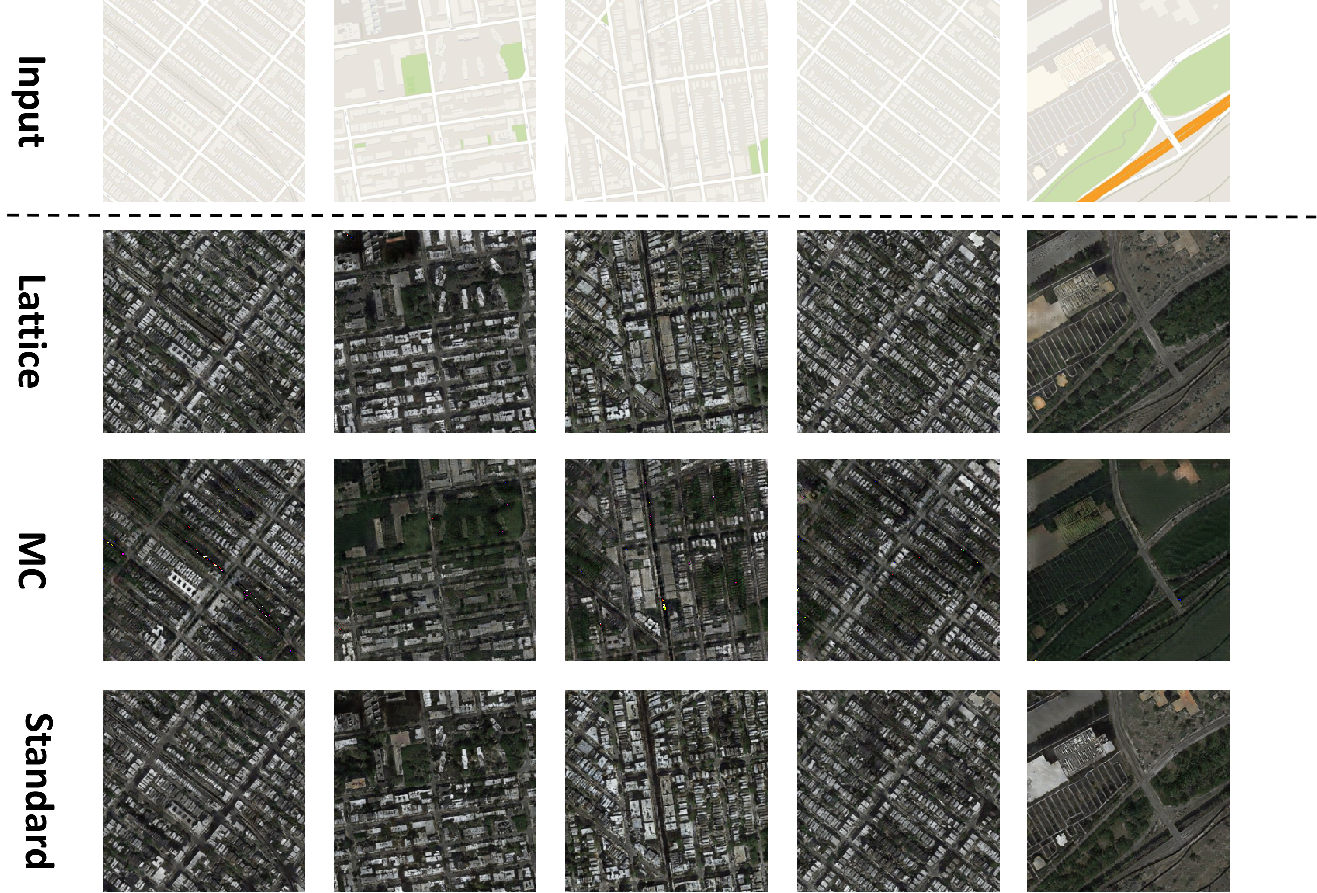
Figure 6: Illustration of the generated images from models trained with subgroup rank-1 lattice sampling, Monte-Carlo sampling, and Standard version of CycleGAN.

References

- [1] Bouhari Arouna. Adaptative monte carlo method, a variance reduction technique. Monte Carlo Methods and Applications, 10(1):1–24, 2004.
- [2] Haim Avron, Vikas Sindhwani, Jiyan Yang, and Michael W Mahoney. Quasi-monte carlo feature maps for shift-invariant kernels. The Journal of Machine Learning Research, 17(1):4096–4133, 2016.
- [3] Matthew James Beal et al. Variational algorithms for approximate Bayesian inference. university of London London, 2003.
- [4] Jean Bourgain, Alexey A Glibichuk, and SERGEI VLADIMIROVICH KONYAGIN. Estimates for the number of sums and products and for exponential sums in fields of prime order. Journal of the London Mathematical Society, 73(2):380–398, 2006.
- [5] Alexander Buchholz, Florian Wenzel, and Stephan Mandt. Quasi-monte carlo variational inference. arXiv preprint arXiv:1807.01604, 2018.
- [6] Krzysztof Choromanski and Vikas Sindhwani. Recycling randomness with structure for sublinear time kernel expansions. 2016.
- [7] Sabrina Dammertz and Alexander Keller. Image synthesis by rank-1 lattices. In Monte Carlo and Quasi-Monte Carlo Methods 2006, 2008.
- [8] Josef Dick, Frances Y Kuo, and Ian H Sloan. High-dimensional integration: the quasi-monte carlo way. Acta Numerica, 22:133–288, 2013.
- [9] Carola Doerr and François-Michel De Rainville. Constructing low star discrepancy point sets with genetic algorithms. In Proceedings of the 15th annual conference on Genetic and evolutionary computation, pages 789–796, 2013.
- [10] David Steven Dummit and Richard M Foote. Abstract algebra, volume 3. Wiley Hoboken, 2004.
- [11] Leonhard Grünschloß, Johannes Hanika, Ronnie Schwede, and Alexander Keller. (t, m, s)-nets and maximized minimum distance. In Monte Carlo and Quasi-Monte Carlo Methods 2006, pages 397–412. Springer, 2008.
- [12] John Hammersley. Monte carlo methods. Springer Science & Business Media, 2013.
- [13] L-K Hua and Yuan Wang. Applications of number theory to numerical analysis. Springer Science & Business Media, 2012.
- [14] Herve Jegou, Matthijs Douze, and Cordelia Schmid. Product quantization for nearest neighbor search. IEEE transactions on pattern analysis and machine intelligence, 33(1):117–128, 2010.
- [15] Diederik P Kingma and Max Welling. Auto-encoding variational bayes. arXiv preprint arXiv:1312.6114, 2013.
- [16] AN Korobov. The approximate computation of multiple integrals. In Dokl. Akad. Nauk SSSR, volume 124, pages 1207–1210, 1959.
- [17] Nikolai Mikhailovich Korobov. Properties and calculation of optimal coefficients. In Doklady Akademii Nauk, volume 132, pages 1009–1012. Russian Academy of Sciences, 1960.
- [18] Helene Laimer. On combined component-by-component constructions of lattice point sets. Journal of Complexity, 38:22–30, 2017.
- [19] Quoc Le, Tamás Sarlós, and Alex Smola. Fastfood-approximating kernel expansions in loglinear time. In Proceedings of the international conference on machine learning, 2013.
- [20] Pierre L’ecuyer and David Munger. Algorithm 958: Lattice builder: A general software tool for constructing rank-1 lattice rules. ACM Transactions on Mathematical Software (TOMS), 42(2):1–30, 2016.
- [21] Gunther Leobacher and Friedrich Pillichshammer. Introduction to quasi-Monte Carlo integration and applications. Springer, 2014.
- [22] James N Lyness. Notes on lattice rules. Journal of Complexity, 19(3):321–331, 2003.
- [23] Yueming Lyu. Spherical structured feature maps for kernel approximation. In Proceedings of the 34th International Conference on Machine Learning-Volume 70, pages 2256–2264, 2017.
- [24] Alireza Makhzani, Jonathon Shlens, Navdeep Jaitly, Ian Goodfellow, and Brendan Frey. Adversarial autoencoders. arXiv preprint arXiv:1511.05644, 2015.
- [25] Harald Niederreiter. Random number generation and quasi-Monte Carlo methods, volume 63. Siam, 1992.
- [26] Dirk Nuyens and Ronald Cools. Fast algorithms for component-by-component construction of rank-1 lattice rules in shift-invariant reproducing kernel hilbert spaces. Mathematics of Computation, 75(254):903–920, 2006.
- [27] Art B Owen. Monte carlo book: the quasi-monte carlo parts. 2019.
- [28] Farhad Pourkamali-Anaraki, Stephen Becker, and Michael B Wakin. Randomized clustered nystrom for large-scale kernel machines. In Thirty-Second AAAI Conference on Artificial Intelligence, 2018.
- [29] Ali Rahimi and Benjamin Recht. Random features for large-scale kernel machines. In Advances in neural information processing systems, 2007.
- [30] Tim Salimans, Jonathan Ho, Xi Chen, Szymon Sidor, and Ilya Sutskever. Evolution strategies as a scalable alternative to reinforcement learning. arXiv preprint arXiv:1703.03864, 2017.
- [31] Ilya D Shkredov. On exponential sums over multiplicative subgroups of medium size. Finite Fields and Their Applications, 30:72–87, 2014.
- [32] I Sloan and A Reztsov. Component-by-component construction of good lattice rules. Mathematics of Computation, 71(237):263–273, 2002.
- [33] Ian H Sloan and Henryk Woźniakowski. Tractability of multivariate integration for weighted korobov classes. Journal of Complexity, 17(4):697–721, 2001.
- [34] Anthony Tompkins, Ransalu Senanayake, Philippe Morere, and Fabio Ramos. Black box quantiles for kernel learning. In The 22nd International Conference on Artificial Intelligence and Statistics, pages 1427–1437, 2019.
- [35] Jiyan Yang, Vikas Sindhwani, Haim Avron, and Michael Mahoney. Quasi-monte carlo feature maps for shift-invariant kernels. In International Conference on Machine Learning, pages 485–493, 2014.
- [36] Jun-Yan Zhu, Taesung Park, Phillip Isola, and Alexei A Efros. Unpaired image-to-image translation using cycle-consistent adversarial networks. In Proceedings of the IEEE international conference on computer vision, pages 2223–2232, 2017.