Spin and Polarization in High-Energy Hadron-Hadron and Lepton-Hadron Scattering

Abstract

The role of spin degrees of freedom in high-energy hadron-hadron and lepton-hadron scattering is reviewed with emphasis on the dominant role of soft, diffractive, non-perturbative effects. Explicit models based on analyticity and Regge-pole theory, including the pomeron trajectory (gluon exchange in the $t$ channel) are discussed. We argue that there is a single, universal pomeron in Nature, manifest as relatively “soft” or “hard”, depending on the kinematics considered. Both the pomeron and the non-leading (secondary) Regge trajectories, made of quarks are non-linear, complex functions. They are populated by a finite number of resonances: known baryons and mesons in case of the reggeons and hypothetical glueballs in case of the pomeron (“oddballs” on the odderon trajectory). Explicit models and fits are presented that may be used in recovering generalized parton distributions from deeply virtual Compton scattering and electoproduction of vector mesons.

I Introduction

Interest in spin physics at high-energies was varying with time. In general, there is a prejudice that the role of spin decreases as energy is increasing. This may be true in general, especially in hadronic reaction, with some exceptions. First, one has to understand the origin of polarization in the scattering of unpolarized hadrons, as for example in $\Lambda$ production. Another issue is the still purely understood delicate mechanism of the diffraction minimum in high-energy proton-proton scattering. This point will be discussed in Section II. Here one inevitably encounters related problems such as: diffraction and the nature of the pomeron, that could be utilized as made of gluons; reconciling soft (non-perturabative, Regge) and hard (perturbative QCD) aspects of the theory, nucleon structure, revealed in inclusive deep-inelastic scattering (DIS) and exclusive deeply virtual Compton scattering (DVCS) as means to reveal the nucleon structure, closely related to spin and polarization, thus connecting structure and dynamics.

The present paper is a recapitulation of the earlier results by the author, revised, updated and extended with account for the recent developments in the field, especially those connected to “nucleon holography”, based on generalized parton distributions (GPDs). Parallel to these practical developments, the still open basic problem of quark confinement is always present in our discussions.

Due to recent progress in understanding the internal structure of the nucleon, especially connected with deeply virtual Compton scattering (DVCS) and generalized parton distributions (GPD) as well as the prospects of building new experimental facilities, such as the planned Electron Ion Collider (EIC), the interest definitely shifted to lepton induced inelastic reactions.

Recent interest in spin physics was triggered two decades ago by the publication of the EMC data (EMC, ) (so-called “spin crisis”). We briefly mention it in Section VII recommending for further reading the excellent presentation of this issue in Ref. Rev2 .

Since all high-energy processes are dominated by pomeron exchange in the $t$ channel, we pay special attention to the derivation and properties of the pomeron and its relation to gluon exchange, by which we mean the identity/diversity of/between the BFKL pomeron derived from QCD and that based on the analytic $S$ matrix theory. In particular, we discuss the following issues:

• Is the input pomeron a simple Regge pole? What are the alternatives, if any?

• Do resonances terminate, abruptly replaced by a continuum or they gradually fade, their peaks becoming progressively wider and lower? This issue is connected with the Hagedorn spectrum and possible phase transition between hadronic and quark-gluon matter.

• Origin of the diffraction (dip-bump) pattern in elastic hadron scattering;

• Role of unitarization in producing the dip-bump structure;

• Are there two (or more) pomerons—a “soft” and a “QCD-inspired”, “hard” one?

• Can the Regge-pomeron pole be $Q^{2}-$dependent?

The paper is organized as follows. In Section II we discuss elastic $NN$ scattering with spin. Recall that the dominant point of view is that the role of spin decreases as energy increases, and it can be ignored at multi-GeV energies, i.e., beyond those of the ISR, and even more so at the LHC. Spin effect may be important in the region of the diffraction minimum, i.e., around $t=-1$ GeV². The point is that the origin and mechanism of the dip-bump phenomenon is still disputable. There are many models but no theoretical understanding of the origin of this important phenomenon. Predictions, mostly based on variants of the Regge-eikonal approach, failed in predicting the position and depth of the dip at the LHC. Spin effects are not the favourite but still a viable possibility, alternative to the dominant ones, based on unitarity (Section II.3).

The importance and properties of the Regge trajectories are repeatedly stressed throughout this paper, with a dedicated Section II.2. Dual models have shown that Regge trajectories are sort of dynamical variables. The trajectories are non-linear, complex function. Their thresholds and asymptotic behaviour should satisfy known constraints. For example, the lowest, $4m_{\pi}$ threshold affects the behaviour of the differential cross section in the Coulomb interference region, competing with possible spin effects.

In Section III we focus on the procedure of recovering Generalized Parton Distributions (GPDs) from electron–proton scattering with spin, measured at the JLab Grav . Here again the pomeron exchange is a basic element of the theory. Different from hadron-hadron scattering, dominated by a “soft” pomeron exchange, here the pomeron is “hard”, i.e., its intercept is much larger ($\alpha(0)\approx 1.3)$ than that considered in Section II. In Section IV we introduce a model for Deep Inelastic Scattering (DIS) amplitude with $Q^{2}$-dependent pomeron intercept. That model will be generalized to deeply virtual Compton scattering (DVCS) in Section V, applicable both to “soft”, e.g., $NN$ scattering Section II, and “hard” DVCS.

Various aspects related to the origin of nucleon’s spin are discussed in Section VII. We share the point of view that there is no “crisis”, over-dramatized after the EMS measurements. The proton spin $1/2$ can be collected from that of its constituents and their motion.

Finally, let us mention recent findings in spin physics revealed in ultra-relativistic heavy-ion collisions; STAR collaboration STAR discovered a significantly nonzero global polarization of Lambda hyperons produced in non-central Au–Au collisions in the RHIC Beam Energy Scan (BES) Program STAR . Different hydrodynamic models Karp ; Karp1 ; Karp2 generally reproduce the magnitude of the measured polarization. In the hydrodynamic models, the Lambda hyperons produced at “particlization” (fluid to particle transition) hypersurface acquire polarization via a thermodynamic spin-vorticity coupling mechanism. This effect is interesting as a possible manifestation of the most vortic fluid ever made.

Interestingly, this is not the first case that $\Lambda$ polarization raises interest in the high energy community. In the nineteens of the past century, much discussion was related Lambda to the origin of polarization in the scattering of unpolarized particles. According to Ref. Strum polarization of inclusively produced lambdas arises due to the spin–orbit interaction in a scalar field in which quarks recombine into hadrons.

The present paper to a large extent reflects the author’s vision of the spin effects in the “soft” region and his personal contribution in the field. For a much wider panorama we recommend to the reader the excellent papers Leader0 ; Rev1 ; Rev2 .

II Hadron-Hadron Scattering

In this section we collect the basic notions and rules indispensable in describing hadronic reactions. We restrict our discussion of this vast field to elastic nucleon scattering in the nearly forward region, dominated by the diffraction cone, and nominated “soft” or “non-perturbative”, implying that perturbative QCD methods here are not applicable. Instead, the basic tools are those based on the analytic $S$ matrix, namely, dispersion relations, unitarity and Regge poles. We relate these means in the context of the subject of the present paper—spin and polarization effects at high energies. Below is a short overview of the relevant tools.

Soft events are described by Regge pole models, sometimes appended by “QCD-inspirations”. In most of the papers on the subject, a spin-independent invariant scattering amplitude is used at high-energies. Since spin effects cannot be excluded a priori, below we briefly present an introduction to the relevant formalism.

In the Regge pole model, the trajectories contain most of the basic information on the dynamics. Their form is constrained by unitarity and analyticity, and is intimately connected by the Chew–Frautchi plot to the spectrum of hadrons. This is a central issue in high energy physics, since it is related to the problem of confinement: how do heavy resonances melt producing a quark–gluon soup? In our approach, the real part of Regge trajectories is limited, implying a finite number of resonances in Nature. This issue is related to the Hagedorn spectrum and “ultimate temperature”, now interpreted as a the temperature of the phase transition between hadrons and quark–gluon plasma Biro .

Unitarity is both important and technically difficult to be satisfied. Various approaches and approximations to unitarity are presented and compared in this Section. Let us mention that the final result (construction of a viable scattering amplitude) depends both on the input and subsequent unitarization procedure. The better the input (“born term”), the better are chances for its subsequent successful unitarization: unitarity correction to a reasonable input (for example, a dipole pomeron, reproducing itself under unitarization) are small DP .

II.1 Elastic Proton-Proton Scattering

Elastic proton–proton scattering is described by five helicity amplitudes Lehar ; Lehar1 , that in the Regge limit, $t$ fixed and $s\rightarrow\infty$, can be expressed in terms of the Regge-pole contributions as Capella ; Troshin ; Troshin1 ; Selyugin1 ; Selyugin2

$$\Phi_{\lambda_{1},\lambda_{2},\lambda_{3},\lambda_{4}}(s,t)\approx\sum_{i}g^{i}_{\lambda_{1},\lambda_{2}}(t)g^{i}_{\lambda_{3},\lambda_{4}}(t)[\sqrt{|t|}]^{|\lambda_{1}-\lambda_{2}|+|\lambda_{3}-\lambda_{4}|}\left(\frac{s}{s_{0}}\right)^{\alpha_{i}}(1\pm e^{-i\pi\alpha_{i}}),$$ (1)

where $\alpha_{i}\equiv\alpha_{i}(t)$ are Regge trajectories. In high-energy elastic scattering the dominant trajectory is that of the pomeron. In the simplest case, it is linear, parametrized, for simplicity as $\alpha(t)=\alpha(0)+\alpha^{\prime}t$. We will use also advanced models of Regge trajectories, to be introduced in the next Section II.2. Recently Glueballs it was used to predict glue and oddballs—resonances made of two or three gluons.

The above helicity amplitudes differ only by powers of $\sqrt{t}$ leaving the Regge propagator (i.e., nature of the Regge pole) intact. This means that the addition of spin-flip amplitudes by themselves will not provide the dip mechanism, although they will slightly modify it. The (single) diffraction minimum followed by maximum was shown DP to arise even at the Born level by choosing the pomeron to be a dipole (double Regge pole or dipole pomeron (DP) DP —an interesting and unique alternative to a simple Regge pole). Fits to the the data on $pp$ scattering, including those from the LHC (TOTEM Collaboration) using DP was performed recently DP1 . The global fit to all energies, including the dip-bump is good, although it leaves room for further perfection. Inclusion of the spin-flip component may improve the situation.

In most of the relevant papers the dip-bump structure is generated by unitarity corrections, see Section II.3, although there is no consensus on the details.

The differential cross sections is given by

$$\frac{d\sigma}{dt}=\frac{2\pi}{s^{2}}\left(|\Phi_{1}|^{2}+|\Phi_{2}|^{2}+|\Phi_{3}|^{2}+|\Phi_{4}|^{2}+4|\Phi_{5}|^{2}\right)\,.$$ (2)

The helicity amplitudes can be written as $\Phi_{i}(s,t)=\Phi^{h}_{i}(s,t)+\Phi^{\rm em}_{i}(s,t)e^{\varphi(s,t)}$ , where $\Phi^{h}_{i}(s,t)$ comes from the strong interactions, $\Phi^{\rm em}_{i}(s,t)$ from the electromagnetic interactions and $\varphi(s,t)$ is their interference.

The spin correlation parameters, the analyzing power—$A_{N}$ and the and double-spin parameter $A_{NN}$, can be extracted from experimental measurements:

$$A_{N} = \frac{\sigma(\uparrow)-\sigma(\downarrow)}{\sigma(\uparrow)+\sigma(\downarrow)}=\frac{\Delta\sigma^{s}}{\sigma_{0}}\,,$$ (3)

$$A_{NN} = \frac{\sigma(\uparrow\uparrow)-\sigma(\uparrow\downarrow)}{\sigma(\uparrow\uparrow)+\sigma(\uparrow\downarrow)}=\frac{\Delta\sigma^{d}}{\sigma_{0}}\,,$$ (4)

where $\Delta\sigma^{s}$ and $\Delta\sigma^{d}$ refer to the difference of single- and double-spin-flip cross sections. The expressions for these parameters are

$$A_{N}\frac{d\sigma}{dt} = -\frac{4\pi}{s^{2}}\left[Im(\Phi_{1}+\Phi_{2}+\Phi_{3}-\Phi_{4})\Phi^{*}_{5}\right]\,;$$ (5)

$$A_{NN}\frac{d\sigma}{dt} = \frac{4\pi}{s^{2}}\left[Re(\Phi_{1}\Phi^{*}_{2}-\Phi_{3}\Phi^{*}_{4})+|\Phi_{5}|^{2}\right]\,.$$ (6)

II.2 Regge Trajectories

Unitarity imposes a severe constraint on the threshold behaviour of the trajectories, as shown on the diagram, Figure 1:

$$\Im m\alpha(t)_{t\rightarrow t_{0}}\sim(t-t_{0})^{\Re e\alpha(t_{0})+1/2},$$ (7)

while asymptotically the trajectories are constrained by

$$\Bigg{|}\frac{\alpha(t)}{\sqrt{t}\ln{t}}\Bigg{|}_{t\rightarrow\infty}\leq{\rm const}.$$ (8)

The above asymptotic constraint can be still lowered to a logarithm by imposing wide-angle power behaviour for the amplitude.

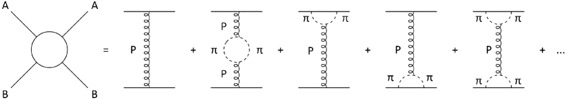
Figure 1: Diagram of elastic scattering with $t$-channel exchange containing a branch point at $t=4m_{\pi}^{2}$.

The trajectory satisfying the above constraints is:

$$\alpha(t)=\frac{1+\delta+\alpha_{1}t}{1+\alpha_{2}\big{(}\sqrt{t_{0}-t}-\sqrt{t_{0}})},$$ (9)

where $t_{0}=4m_{\pi}^{2}$ for the pomeron and $t_{0}=9m_{\pi}^{2}$ for the odderon and $\delta,\alpha_{1},\alpha_{2}$ are parameters fitted to the data with the obvious constraints: $\alpha(0)\approx 1.08$ and $\alpha^{\prime}(0)\approx 0.3$ (in the case of the pomeron trajectory). Trajectory (9) has square-root asymptotic behaviour, in accordance with the requirements of the analytic $S$-matrix theory.

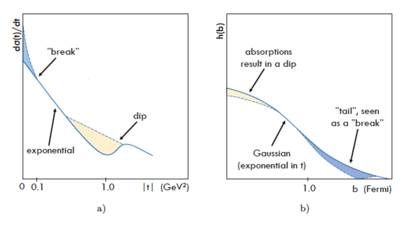
Figure 2: (a) Typical shape of the high-energy differential (diffractive) cross section, and (b) Its impact-parameter image. A “dictionary” relating the shape of the diffraction cone (in $t$), left icon to its impact-paramter image (rignt), and highlighting their two silent features: the “break”, origin of nucleon’s atmosphere and the dip-bump, resulting from absorptions (unitarity!) at small values of the impact parameter, see DP .

The contribution of the lowest threshold in the $t$ channel of the trajectory and the scattering amplitude is shown on the diagram, Figure 1. The presence of this threshold produces a “break” in the diffraction cone and generates the pion cloud of the nucleon, as shown in Figure 2.

For $t>>t_{0},\ \ |\alpha(t)|\rightarrow\frac{\alpha_{1}}{\alpha_{2}}\sqrt{|t|}$. For $t>t_{0}$ (on the upper edge of the cut), $\Im m\alpha>0.$

The intercept is $\alpha(0)=1+\delta$ and the slope at $t=0$ is

$$\alpha^{\prime}(0)=\alpha_{1}+\alpha_{2}\frac{1+\delta}{2\sqrt{t_{0}}}.$$ (10)

Resonances terminate, i.e., they do not appear beyond the maximum value or the finite real part of a given Regge trajectory.

For a recent application of this trajectory to glueball spectroscopy see Ref. Glueballs .

II.3 Unitarity

The best known unitarization procedure is that of Regge-eikonal, where the input (“Born term”) is a Regge-pole amplitude.

It implies two Fourier–Bessel transforms (integrals), one from the Mandelstam variable $t$ (momentum space) to the impact parameter $b$ (coordinate space). While direct integration is usually performed analytically (trivial for linear Regge trajectories and still simple for a single square-root threshold, see Ref. NC , the inverse integral is much more cumbersome, and can be done only numerically. The technicalities become even more complicated when spin degrees are included (see below).

A simple unitarization procedures is by the use Selyugin1 ; Selyugin2 of the equation:

$$\frac{dN}{dy}=\Delta N\ [\ 1-N\ ]\,,$$ (11)

where $y=\log(s/s_{0})$ and $\Delta=1-\alpha(0)$, ($\alpha(0)$ is the intercept of the leading Regge pole trajectory.

Its solution is

$$N=\frac{\chi(s,b)}{1\ +\ \chi(s,b)}\,,$$ (12)

where $\chi(s,b)\approx s^{\Delta}$ is connected with the Born term of the scattering amplitude.

The scattering amplitude is

$$\Phi^{h}(s,t)\ =\ \frac{i}{2\pi}\ \int\ d^{2}b\ e^{i\vec{b}\vec{q}}\frac{\chi(s,b)}{1+\chi(s,b)}\,.$$ (13)

The phase $\chi(s,b)$ is connected to the interaction potential:

$$\chi(s,b)\ =\ F_{\rm Born}(s,b)\ \approx\frac{1}{k}\ \int\hat{V}\left(\sqrt{b^{2}+z^{2}}\right)dz.$$ (14)

If the potential contains a non-spin-flip part and, for example, spin-orbital and spin-spin interactions, the phase is:

$$\chi(s,b)=\chi_{0}(s,b)-i\ \vec{n}\cdot(\vec{\sigma}_{1}+\vec{\sigma}_{2})\chi_{\rm LS}(s,b)-i(\vec{\sigma}_{1}\cdot\vec{\sigma}_{2})\ \chi_{\rm SS}(s,b).$$ (15)

If however only the spin-flip and spin-non-flip parts are accounted for, the overlap function is

$$\Gamma(s,b)=\frac{\chi_{0}(s,b)+\sigma\chi_{sf}(s,b)}{1+\chi_{0}(s,b)+\sigma\chi_{sf}(s,b)}=1-\frac{\left(1+\chi_{0}(s,b)\right)-\sigma\chi_{sf}(s,b)}{\left(1+\chi_{0}(s,b)\right)^{2}-\left(\sigma\chi_{sf}(s,b)\right)^{2}}\,.$$ (16)

Using the representation for the Bessel functions

$$J_{0}(x)\ =\frac{1}{2\pi}\ \int_{0}^{2\pi}\ e^{ix\cos\phi}\ d\phi\ \ \ \ \ J_{1}(x)\ =-\frac{1}{2\pi}\ \int_{0}^{2\pi}\ e^{ix\cos\phi}\ \sin{\phi}\ d\phi\,,$$ (17)

the representation of spin-non-flip and spin flip amplitude becomes

$$\Phi^{h}_{1}(s,t)\ =\ i\ \int_{0}^{\infty}\ bJ_{0}(bq)\frac{\chi_{0}(s,b)}{1+\chi_{0}(s,b)}db\,;$$ (18)

$$\Phi^{h}_{5}(s,t)\ =\ i\ \int_{0}^{\infty}\ b^{2}J_{1}(bq)\frac{\chi_{sf}(s,b)}{\left(1+\chi_{0}(s,b\right))^{2}}db\,.$$ (19)

II.3.1 “$U$-matrix” Unitarization

With an extra coefficient $n$

$$\frac{dN}{dy}=\Delta N\ [\ 1-N/n\ ]\,.$$ (20)

one gets the so-called $U$-matrix unitarization form, see Troshin and references therein.

This way of unitarization, developed mainly in Serpukhov, Dubna and Kiev, is less familiar than the eikonal one, nevertheless it results in a number of interesting predictions, among which is the so-called reflective scattering Troshin2 , resulting in an increasing ratio $\sigma_{el}(s)/\sigma_{tot}(s)$ at the LHC. The unorthodox predictions of the $U$ matrix approach may bringing new ideas in the complicated field of “soft physics”.

In the impact parameter representation, the properties of the $U$-matrix were explored in Ref. Troshin . In that approach, the hadronic amplitude is given by

$$\Phi^{h}(s,t)\ =\ \frac{i}{2\pi}\ \int\ d^{2}b\ e^{i\vec{b}\vec{q}}\frac{\chi(s,b)}{1+\chi(s,b)/2}\,,$$ (21)

where $\chi(s,b)$ is the same Born amplitude as before.

Comparing Equation (21) with Equation (13), we see that they are of similar rational form, just they differ by the additional coefficient in the denominator. This additional coefficient leads to different analytic properties: the upper bound at which the overlapping function saturates will be twice that compared with the eikonal or the $U_{e}$ representations, and the inelastic overlap function at $b=0$ tends to zero at high energies. Furthermore, $\sigma_{\rm el}/\sigma_{\rm tot}\rightarrow 1$.

For the $pp$ helicity amplitudes the solution of the unitarity equations is Troshin :

$$\Phi_{\lambda_{3},\lambda_{4},\lambda_{1},\lambda_{2}}({\bf p},{\bf q}) = U_{\lambda_{3},\lambda_{4},\lambda_{1},\lambda_{2}}({\bf p},{\bf q})+$$

$$i\frac{\pi}{8}\sum_{\lambda^{\prime},\lambda^{\prime\prime}}\int d\Omega_{{\bf\hat{k}}}U_{\lambda_{3},\lambda_{4},\lambda^{\prime},\lambda^{\prime\prime}}({\bf p},{\bf k})\Phi_{\lambda^{\prime},\lambda^{\prime\prime},\lambda_{1},\lambda_{2}}({\bf k},{\bf q})\,,$$

II.3.2 Eikonal

To get the standard eikonal representation of the elastic scattering amplitude in the impact parameter representation one uses the non-linear equation

$$\frac{dN_{e}}{dy}=-\Delta\log(1-N_{e})[1-N_{e}]\,.$$ (23)

where $y=\log(s/s_{0})$ and the subscript “e“ implies that the solution $N_{e}$ is of the standard eikonal form

$$N_{e}=\Gamma(s,b)=[1-e^{-\chi(s,b)}].$$ (24)

The eikonal representation is then

$$\Phi^{h}(s,t)\ =\frac{i}{2\pi}\ \int\ e^{i\vec{b}\vec{q}}\ \left[1-e^{-\chi(s,b)}\right]\ d^{2}b,$$ (25)

where:

$$\chi(s,b)=\chi_{0}(s,b)-i\ \vec{n}\cdot(\vec{\sigma}_{1}+\vec{\sigma}_{2})\chi_{LS}(s,b)-i(\vec{\sigma}_{1}\cdot\vec{\sigma}_{2})\ \chi_{SS}(s,b).$$ (26)

With account for Equations (17) and (27), one gets respectively for spin non-flip and spin-flip

$$\Phi^{h}_{1}(s,t)\ =\ i\ \int_{0}^{\infty}\ bJ_{0}(bq)\left[1-e^{\chi_{0}(s,b)}\right]\ \left[1-b^{2}\chi^{2}_{\rm LS}(s,b)-3/2\chi^{2}_{\rm SS}(s,b)\right]\ db,$$ (27)

$$\Phi^{h}_{5}(s,t)\ =\ i\ \int_{0}^{\infty}\ J_{1}(bq)\chi_{1}e^{\chi_{0}(s,b)}\ b\ \left[\chi_{\rm LS}(s,b)+i\ \chi_{\rm LS}(s,b)\ \chi_{\rm SS}(s,b)\right]\ db,$$ (28)

where

$$\chi(s,b)_{0} \approx \ \int_{-\infty}^{\infty}V_{0}(s,b,z)dz\,;$$ (29)

$$\chi(s,b)_{1} \approx \frac{b}{2}\ \int_{-\infty}^{\infty}V_{1}(s,b,z)dz\,.$$ (30)

For Gaussian potentials $V_{0}$ and $V_{1}$

$$V(s,b)_{0,1}\ \approx\ \int_{-\infty}^{\infty}e^{-Br^{2}}\ dz=\frac{\sqrt{\pi}}{\sqrt{B}}e^{-Bb^{2}}\,,$$ (31)

in the first Born approximation, $\Phi_{0}^{h}$ and $\Phi_{1}^{h}$ take the forms

$$\Phi^{h}_{1}(s,t)\ \approx\ \int_{0}^{\infty}\ bJ_{0}(bq)e^{-Bb^{2}}db=e^{-Bq^{2}};$$ (32)

$$\Phi^{h}_{5}(s,t)\ \approx\ \int_{0}^{\infty}\ b^{2}J_{1}(bq)e^{-Bb^{2}}db=qBe^{-Bq^{2}}.$$ (33)

In view of these technical complications, of interest is the unique case of a dipole pomeron (DP), reproducing itself under eikonal corrections, as noticed in Ref. Phillips , see also the Appendix in Fortschritte . In other words, DP in the impact parameters representation remains stable (intact) under eikonalization. In addition, a DP produces logarithmically rising cross sections at unit pomeron intercept and obeys geometrical scaling, making it attractive as an efficient model of diffraction. Note that higher order Regge poles violate unitarity.

III Nuclear Structure: From Deeply Virtual Compton Scattering (DVCS) to Generalized Parton Distributions (GPDs)

An important part of spin physics is lepton-hadron scattering. Deeply virtual exclusive $ep$ processes provide an important tool in accessing the generalized parton distributions (GPDs) Mueller:1998fv ; Radyushkin:1996nd ; Ji:1996nm . The underlying mechanism is Regge-pole exchange in the $t$-channel. Based on factorization theorems Collins:1996fb ; Collins:1998be , GPDs offer a partonic interpretation of these processes, where unobserved transverse degrees of freedom are integrated out. Thereby, these universal functions, defined in terms of matrix elements of quark and gluon operators or, alternatively, as a non-diagonal overlap of light-cone wave functions  Diehl:1998kh ; Diehl:2000xz , encode the non-perturbative aspects of the nucleon Diehl:2003ny ; Belitsky:2005qn . In particular, GPDs provide access to the transverse spatial distribution of patrons Burkardt:2000za ; Die02 ; KogSop70 , and to the decomposition of the nucleon spin in terms of quark and gluon degrees of freedom Ji:1996ek .

Phenomenologically, exclusive electroproduction of a real photon, DVCS, depicted in Figure 3 (left), is the golden channel to constrain GPDs as it is theoretically clean and the phase of its amplitude can be measured using the interference with the Bethe–Heitler (BH) amplitude (see Figure 3; cf. Figures 4 and 5).

More details, especially those related to experiments can be found in Accardi:2012hwp ; Fazio .

III.1 Deeply Virtual Compton Scattering

The differential photon electroproduction cross section is the sum of the BH amplitude squared, DVCS amplitude squared, and the interference (INT) terms (see Figure 4)

$$\frac{d\sigma^{ep\to ep\gamma}}{dx_{\rm B}dtd{\cal Q}^{2}d\phi d\varphi}=\frac{d\sigma^{ep\to ep\gamma,\mbox{\tiny BH}}(F_{1},F_{2})}{dx_{\rm B}dtd{\cal Q}^{2}d\phi d\varphi}\pm\frac{d\sigma^{ep\to ep\gamma,\mbox{\tiny INT}}(F_{1},F_{2},{\cal F})}{dx_{\rm B}dtd{\cal Q}^{2}d\phi d\varphi}+\frac{d\sigma^{ep\to ep\gamma,\mbox{\tiny(D)VCS}}({\cal F},{\cal F}^{\ast})}{dx_{\rm B}dtd{\cal Q}^{2}d\phi d\varphi}\,.$$ (34)

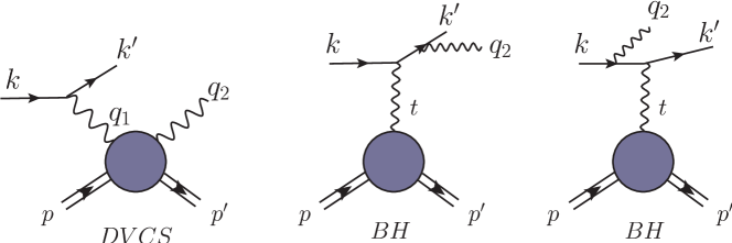
Figure 3: Deeply virtual Compton scattering (DVCS) and Bethe–Heitler (BH) amplitudes contributing to the photon leptoproduction cross section in leading order approximation of QED.

Here the $+(-)$ signs correspond to the electron (positron) beam, $x_{\rm B}$ is the common Bjorken scaling variable, $\phi$ is the azimuthal angle between lepton and hadron scattering planes, and $\varphi=\Phi-\phi$, where $\Phi(\equiv\phi_{S})$ is the angle between the lepton scattering plane and a possible transverse spin component of the incoming proton at rest. To the leading order (LO) in the electromagnetic fine structure constant $\alpha_{\rm em}=\frac{e^{2}}{4\pi}\approx\frac{1}{137},$ and neglecting the electron mass, the three terms on the r.h.s. of (34) are known in terms of the electromagnetic Pauli form factor $F_{1}(t)$ and the Dirac form factor $F_{2}(t)$, parameterizing the BH amplitude, and a set of 12 photon helicity dependent CFFs ${\cal F}_{ab}(x_{\rm B},t,{\cal Q}^{2})$, parameterizing the DVCS amplitude, see Figure 3. These CFFs are labelled by the helicities of the incoming $a\in\{+,0,-\}$ and outgoing photon $b\in\{+,-\}$ called

$${\cal F}_{ab}\in\{{\cal H}_{ab},{\cal E}_{ab},\widetilde{\cal H}_{ab},\widetilde{\cal E}_{ab}\}\quad\mbox{with}\quad{\cal F}_{0-}={\cal F}_{0+}\,,\quad{\cal F}_{+-}={\cal F}_{-+}\,,$$ (35)

Figure 4: Interference in DVCS (Equation (34)) provides a holographic picture of the proton similar to the classical one.

Figure 5: Generalized parton distributions (GPD) (right) unify in a non-trivial way the the impact parameter image of a nucleon (left) with the $x$ dependence of DIS structure functions (middle).

III.2 Relating DVCS Observables to GPDs

GPDs, denoted as

$$F(x,\eta=\xi,t,\mu^{2})\quad\mbox{with}\quad F\in\{H,E,\widetilde{H},\widetilde{E}\}\,,$$

besides depending on the partonic momentum fraction $x$ and the momentum transfer squared $t$, depend also on the $t$-channel longitudinal momentum fraction $\eta$, called skewness (often denoted by $\xi$ in the literature), and on the factorization scale $\mu^{2}$. The unpolarized parton GPDs are called $H$ and $E$ Ji:1998pc , where the former (latter) GPD can be loosely associated with a proton helicity (non)conserved distribution.

DVCS observables can be evaluated in terms of the helicity CFFs (35). To express them in terms of GPDs, it is appropriate to utilize a conventionally defined GPD-inspired CFF basis, such as the one introduced in Belitsky:2001ns :

$${\cal F}\in\{{\cal H},{\cal E},\widetilde{\cal H},\widetilde{\cal E},{\cal H}_{3},{\cal E}_{3},\widetilde{\cal H}_{3},\widetilde{\cal E}_{3},{\cal H}_{\rm T},{\cal E}_{\rm T},\widetilde{\cal H}_{\rm T},\widetilde{\cal E}_{\rm T}\}\,.$$ (36)

Here, the CFFs ${\cal H},{\cal E},\widetilde{\cal H}$, and $\widetilde{\cal E}$ are associated with twist-two GPDs $F\in\{H,E,\widetilde{H},\widetilde{E}\}$ and govern the photon helicity non-flip DVCS amplitude, i.e., at leading twist-two accuracy one has

$${\cal F}_{++}(x_{\rm B},t,{\cal Q}^{2})={\cal F}(x_{\rm B},t,{\cal Q}^{2})+{\cal O}(1/{\cal Q}^{2})\quad\mbox{for}\quad{\cal F}\in\{{\cal H},{\cal E},\widetilde{\cal H},\widetilde{\cal E}\}.$$ (37)

To LO they are calculated from the handbag diagram, depicted in Figure 6, yielding the convolution formula

$${\cal F}(x_{\rm B},t,{\cal Q}^{2})\stackrel{{\scriptstyle\rm LO}}{{=}}\sum\limits_{i}\int_{-1}^{1}\!dx\left[\frac{e^{2}_{i}}{\xi-x-i\epsilon}\mp\{x\rightarrow-x\}\right]F_{i}(x,\xi,t,\mu^{2})\;\;\mbox{for}\;\;{\cal F}\in\left\{{{\cal H},{\cal E}\atop\widetilde{\cal H},\widetilde{\cal E}}\right\},$$ (38)

where $e_{i}$ are the fractional quark charges. The variable $\xi\sim x_{\rm B}/(2-x_{\rm B})$ is a conventionally defined Bjorken-like scaling variable, equated to the longitudinal momentum fraction in the $t$-channel, and $\mu^{2}\sim{\cal Q}^{2}$ being the factorization scale.

For twist-two and LO accuracy, and light quarks one adopts the conventions

$$\xi=\frac{x_{\rm B}}{2-x_{\rm B}}\quad\mbox{and}\quad\mu^{2}={\cal Q}^{2}\,.$$ (39)

From Regge-pole models, consistent with the data, see Section IV below, the real part of the dominant CFF ${\cal H}$ in the small- and even moderate-$x_{\rm B}$ region is much smaller than its imaginary part (at least for smaller values of $-t$). One concludes that the interference term is negligible and one can simplify the $t$-differential cross section to

$$\frac{d\sigma^{\mbox{\tiny TOT}}}{dt}\approx\frac{y^{2}\left[\frac{d\sigma_{\rm T}^{\mbox{\tiny BH,red}}}{dt}+\varepsilon(y)\frac{d\sigma_{\rm L}^{\mbox{\tiny BH,red}}}{dt}\right]}{\left(1-y\frac{(1-x_{\rm B})t}{{\cal Q}^{2}+t}\right)\left(\frac{{\cal Q}^{2}+t}{{\cal Q}^{2}+x_{\rm B}t}-y\right)}+\frac{d\sigma^{\mbox{\tiny\rm DVCS}}(y)}{dt}$$ (40)

with $\frac{d\sigma^{DVCS}(y)}{dt}=\frac{d\sigma_{T}^{DVCS}}{dt}+\varepsilon(y)\frac{d\sigma_{L}^{DVCS}}{dt}.$

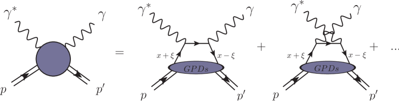
Figure 6: Factorization of the DVCS amplitude to leading order in perturbative QCD and to leading twist-two accuracy.

IV Modelling DVCS

Below we present models of DVCS and vector meson production (VMP), potentially useful in calculating GPDs.

Regge pole models provide an adequate framework to describe high-energy, low $t$ scattering phenomena. Being part of the $S$ matrix theory, however, strictly speaking, they are valid only for the scattering of on-mass-shall particles. Still, the successful application of the Regge pole models in describing the off-mass-shall HERA data opened the way to their use in deep-inelastic scattering, DVCS and vector meson production at HERA. Off-shell extension was realized e.g., by calling the $Q^{2}$-dependent Regge trajectories “effective” ones. A particularly simple and efficient Regge pole model Capua with $Q^{2}$-dependent residues (vertices) is presented below, in Section IV.

In a more advanced Regge-pole model, Section V the Regge trajectories and the residues do not depend on virtuality. Instead, the amplitude contains two (or more) Regge-pole terms, whose relative weight depends on $Q^{2}$, mimicking the multi-pole nature of the so-called QCD pomeron.

Simple Model of DVCS

By Regge factorization, Figure 7, the DVCS amplitude can be written as

$$A(s,t,Q^{2})_{\gamma^{*}p\rightarrow\gamma p}=-A_{0}V_{1}(t,Q^{2})V_{2}(t)(-is/s_{0})^{\alpha(t)},$$ (41)

where $A_{0}$ is a normalization factor, $V_{1}(t,Q^{2})$ is the $\gamma^{*}P\gamma$ vertex, $V_{2}(t)$ is the $pPp$ vertex and $\alpha(t)$ is the exchanged pomeron trajectory, which we assume to be logarithmic:

$$\alpha(t)=\alpha(0)-\alpha_{1}\ln(1-\alpha_{2}t).$$ (42)

Such a trajectory is nearly linear for small $|t|$, thus reproducing the forward cone of the differential cross section, while its logarithmic asymptotic provides for the large-angle scaling behaviour, typical of hard collisions at small distances, with power-law fall-off in $|t|$, compatible with the quark counting rules. Here we are referring to the dominant pomeron contribution eventually appended by a secondary trajectory, e.g., the $f$-Reggeon.

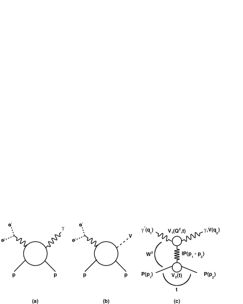
Figure 7: Diagrams of DVCS (a) and VMP (b); (c) DVCS (VMP) amplitude in a Regge-factorized form.

For convenience, and following the arguments based on duality, the $t$ dependence of the $pPp$ vertex is introduced via the $\alpha(t)$ trajectory: $V_{2}(t)=e^{b\alpha(t)}$ where $b$ is a parameter. A generalization of this concept will be applied also to the upper, $\gamma^{*}P\gamma$ vertex by introducing the trajectory

$$\beta(z)=\alpha(0)-\alpha_{1}\ln(1-\alpha_{2}z),$$ (43)

where the value of the parameter $\alpha_{2}$ may be different in $\alpha(t)$ and $\beta(z)$ (a relevant check will be possible when more data are available).

Hence the scattering amplitude, with correct signature, becomes

$$A(s,t,Q^{2})_{\gamma^{*}p\rightarrow\gamma p}=-A_{0}e^{b\alpha(t)}e^{b\beta(z)}(-is/s_{0})^{\alpha(t)}=-A_{0}e^{(b+L)\alpha(t)+b\beta(z)},$$ (44)

where $L\equiv\ln(-is/s_{0})$.

The model contains a limited number of parameters. Moreover, most of them can be estimated a priori. The product $\alpha_{1}\alpha_{2}$ is just the forward slope $\alpha^{\prime}$ of the Reggeon ($\approx$0.2 GeV^-2 for the pomeron, but much higher for $f$ and/or for an effective Reggeon). The value of $\alpha_{1}$ can be estimated from the wide-angle quark counting rules. For large $t$ ($|t|>>$1 GeV²) the amplitude goes roughly as $\sim e^{-\alpha_{1}\ln(-t)}=(-t)^{\alpha_{1}},$ where the power $\alpha_{1}$ is related to the number of quarks in a collision.

From Equation (44) the slope of the forward cone is

$$B(s,Q^{2},t)=\frac{d}{dt}\ln|A|^{2}=2\left[b+\ln\left({s\over{s_{0}}}\right)\right]{\alpha^{\prime}\over{1-\alpha_{2}t}}+2b\,{\alpha^{\prime}\over{1-\alpha_{2}z}},$$ (45)

which, in the forward limit, $t=0$ reduces to

$$B(s,Q^{2})=2\left[b+\ln\left({s\over{s_{0}}}\right)\right]\alpha^{\prime}+2b\,{\alpha^{\prime}\over{1+\alpha_{2}Q^{2}}}.$$ (46)

Thus, the slope shows shrinkage in $s$ and antishrinkage in $Q^{2}.$

In the $Q^{2}\rightarrow 0$ limit the Equation (44) becomes

$$A(s,t)=-A_{0}e^{2b\alpha(t)}(-is/s_{0})^{\alpha(t)}$$ (47)

where we recognize a typical Regge-behaved photoproduction (or, for $Q^{2}\rightarrow m_{H}^{2},$ on-shell hadronic ($H$)) amplitude. The related deep inelastic scattering structure function is recovered by setting $Q_{2}^{2}=Q^{2}_{1}=Q^{2}$ and $t=0$, to get a typical elastic virtual forward Compton scattering amplitude:

$$A(s,Q^{2})=-A_{0}e^{b(\alpha(0)-\alpha_{1}\ln(1+\alpha_{2}Q^{2}))}e^{(b+\ln(-is/s_{0}))\alpha(0)}\propto-(1+\alpha_{2}Q^{2})^{-\alpha_{1}}(-is/s_{0})^{\alpha(0)}.$$ (48)

In the Bjorken limit, when both $s$ and $Q^{2}$ are large and $t=0$ (with $x\approx Q^{2}/s$ valid for large $s$), the structure function is given by:

$$F_{2}(s,Q^{2})\approx{(1-x)Q^{2}\over{\pi\alpha_{e}}}\Im A(s,Q^{2})/s,$$ (49)

where $\alpha_{e}$ is the electromagnetic coupling constant and the normalization is $\sigma_{t}(s)=\frac{4\pi}{s}\Im A(s,Q^{2}).$ The resulting structure function has correct (required by gauge invariance) $Q^{2}\rightarrow 0$ limit and approximate scaling (in $x$) behavior for large enough $s$ and $Q^{2}$.

V Reggeometry

In a series of papers (see Refs. Salii1 ; Salii2 ), photon virtuality was incorporated in a “geometrical” way, reflecting the observed trend in the decrease of the forward slope as a function of $\widetilde{Q^{2}}$. This geometrical approach, combined with the Regge-pole model, was named “Reg-ge-ometry” (a wordplay, pun). A Reggeometric amplitude dominated by a single pomeron shows reasonable agreement with the HERA data on VMP and DVCS, when fitted separately to each reaction.

As further step, to reproduce the observed trend of hardening as $\widetilde{Q^{2}}$ increases, and following Donnachie and Landshoff DL1 ; DL2 , a two-term amplitude, characterized by a two-component—“soft” + “hard”—pomeron, was suggested Salii1 . We stress that the pomeron is unique, but we construct it as a sum of two terms. Then, the amplitude is defined as

$$A(\widetilde{Q^{2}},s,t)=A_{s}(\widetilde{Q^{2}},s,t)+A_{h}(\widetilde{Q^{2}},s,t)$$ (50)

($s=W^{2}$ is the square of the c.m.s. energy), such that the relative weight of the two terms changes with $\widetilde{Q^{2}}$ in the right way, i.e., the ratio $r=A_{h}/A_{s}$ increases as the reaction becomes “harder” and v.v. It is interesting to note that this trend is not guaranteed “automatically”: both the “scaling” model Capua or the Reggeometric one Salii1 ; Salii2 show the opposite tendency, that may not be merely an accident and whose reason should be better understood. This “wrong” trend can and should be corrected, and in fact it was corrected DL1 ; DL2 by means of additional $\widetilde{Q^{2}}$-dependent factors $H_{i}(\widetilde{Q^{2}}),\ i=s,h$ modifying the $\widetilde{Q^{2}}$ dependence of the amplitude, in a such way as to provide increasing of the weight of the hard component with increasing $\widetilde{Q^{2}}$. To avoid conflict with unitarity, the rise with $\widetilde{Q^{2}}$ of the hard component is finite (or moderate), and it terminates at some saturation scale, whose value is determined phenomenologically. In other words, the “hard” component, invisible at small $\widetilde{Q^{2}}$, gradually takes over as $\widetilde{Q^{2}}$ increases. An explicit example of these functions is presented below.

Recall that the invariant scattering amplitude is defined as

$$A(Q^{2},s,t)=\widetilde{H}e^{-\frac{i\pi\alpha(t)}{2}}\left(\frac{s}{s_{0}}\right)^{\alpha(t)}e^{2\left(\frac{a}{\widetilde{Q^{2}}}+\frac{b}{2m_{N}^{2}}\right)t},$$ (51)

where

$$\alpha(t)=\alpha_{0}+\alpha^{\prime}t$$ (52)

is the linear pomeron trajectory (the use of more advanced, non-linear trajectories of Section II.2 is straightforward), $a$ and $b$ are two parameters to be determined from the fitting procedure and $m_{N}$ is the nucleon mass. The coefficient $\widetilde{H}$ is a function providing the right behavior of elastic cross sections in $\widetilde{Q^{2}}$:

$$\widetilde{H}\equiv\widetilde{H}(\widetilde{Q^{2}})=\frac{\widetilde{A_{0}}}{\left(1+\frac{\widetilde{Q^{2}}}{{Q_{0}^{2}}}\right)^{n_{s}}},$$

where $\widetilde{A_{0}}$ is a normalization factor, $Q_{0}^{2}$ is a scale for the virtuality and $n_{s}$ is a real positive number.

In this model one uses an effective pomeron, which can be “soft” or “hard”, depending on the reaction and/or kinematic region defining its “hardness”. In other words, the  values of the parameters $\alpha_{0}$ and $\alpha^{\prime}$ must be fitted to each set of the data. Apart from $\alpha_{0}$ and $\alpha^{\prime}$, the model contains five more sets of free parameters, different in each reaction, as shown in Table 1. The exponent in the exponential factor in Equation (51) reflects the geometrical nature of the model: $a/\widetilde{Q^{2}}$ and $b/2m_{N}^{2}$ correspond to the “sizes” of upper and lower vertices in Figure 7c.

With the norm

$$\frac{d\sigma_{el}}{dt}=\frac{\pi}{s^{2}}|A(Q^{2},s,t)|^{2},$$ (53)

the differential and integrated elastic cross sections become,

$$\frac{d\sigma_{el}}{dt}=\frac{A_{0}^{2}}{\left(1+\frac{\widetilde{Q^{2}}}{{Q_{0}^{2}}}\right)^{2n}}\left(\frac{s}{s_{0}}\right)^{2(\alpha(t)-1)}e^{4\left(\frac{a}{\widetilde{Q^{2}}}+\frac{b}{2m_{N}^{2}}\right)t}$$ (54)

and

$$\sigma_{el}=\frac{A_{0}^{2}}{\left(1+\frac{\widetilde{Q^{2}}}{{Q_{0}^{2}}}\right)^{2n}}\frac{\left(\frac{s}{s_{0}}\right)^{2(\alpha_{0}-1)}}{4\left(\frac{a}{\widetilde{Q^{2}}}+\frac{b}{2m_{N}^{2}}\right)+2\alpha^{\prime}\ln\left(\frac{s}{s_{0}}\right)},$$ (55)

where

$$A_{0}=-\frac{\sqrt{\pi}}{s_{0}}\widetilde{A_{0}}.$$

The results of the fits are presented in Table 1. The “mass parameter” for DVCS was set to $M=0$ GeV, therefore in this case $\widetilde{Q^{2}}=Q^{2}$. Each type of reaction was fitted separately. As it can be seen from the right plot of Figure 8, the single-term model fails to fit both the high- and low-$|t|$ regions properly, especially when soft (photoproduction or low $Q^{2}$) and hard (electroproduction or high $Q^{2}$) regions are considered. One of the problems of the single-term Reggeometric pomeron model, Equation (51), is that the fitted parameters in this model acquire particular values for each reaction,

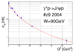
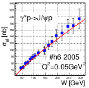
Figure 8: Representative fits of Equations (54) and (55) to the data on $J/\psi$ production. The values of the fitted parameters are compiled in Table 1.

Table 1: Values of the parameters in Equations (54) and (55) fitted to data on vector meson production (VMP) and DVCS at HERA. The parameters with indefinite error bars were fixed at the fitting stage.

	$A_{0}$ $\left[\frac{\sqrt{\text{{nb}}}}{\text{{GeV}}}\right]$	$\widetilde{Q^{2}_{0}}$ $\left[\text{{GeV}}^{\textbf{2}}\right]$	$n$	$\alpha_{0}$	$\alpha^{\prime}$ $\left[\frac{1}{\text{GeV}^{\textbf{2}}}\right]$	$a$	$b$	${\tilde{\chi}}^{2}$
$\rho^{0}$	344 $\pm$ 376	0.29 $\pm$ 0.14	1.24 $\pm$ 0.07	1.16 $\pm$ 0.14	0.21 $\pm$ 0.53	0.60 $\pm$ 0.33	0.9 $\pm$ 4.3	2.74
$\phi$	58 $\pm$ 112	0.89 $\pm$ 1.40	1.30 $\pm$ 0.28	1.14 $\pm$ 0.19	0.17 $\pm$ 0.78	0.0 $\pm$ 19.8	1.34 $\pm$ 5.09	1.22
$J/\psi$	30 $\pm$ 31	2.3 $\pm$ 2.2	1.45 $\pm$ 0.32	1.21 $\pm$ 0.09	0.077 $\pm$ 0.072	1.72	1.16	0.27
$\varUpsilon$(1S)	37 $\pm$ 100	0.93 $\pm$ 1.75	1.45 $\pm$ 0.53	1.29 $\pm$ 0.25	0.006 $\pm$ 0.6	1.90	1.03	0.4
$DVCS$	14.5 $\pm$ 41.3	0.28 $\pm$ 0.98	0.90 $\pm$ 0.18	1.23 $\pm$ 0.14	0.04 $\pm$ 0.71	1.6	1.9 $\pm$ 2.5	1.05

The VMP results clearly show hardening of the pomeron in the change of $\alpha_{0}$ and $\alpha^{\prime}$ when going from light to heavy vector mesons.

It is also interesting to note that the effective pomeron trajectory for DVCS ($\alpha_{0}=1.23,$ $\alpha^{\prime}=0.04$, see Table 1), contrary to expectations is rather “hard”.

Two-Component Reggeometric Pomeron

Now we introduce the universal, “soft” and “hard”, pomeron model. Using the Reggeometric ansatz of Equation (51), we write the amplitude as a sum of two parts, corresponding to the “soft” and “hard” components of a universal, unique pomeron:

$$A(Q^{2},s,t)=\widetilde{H_{s}}\,e^{-i\frac{\pi}{2}\alpha_{s}(t)}\left(\frac{s}{s_{0s}}\right)^{\alpha_{s}(t)}e^{2\left(\frac{a_{s}}{\widetilde{Q^{2}}}+\frac{b_{s}}{2m_{N}^{2}}\right)t}+\widetilde{H_{h}}\,e^{-i\frac{\pi}{2}\alpha_{h}(t)}\left(\frac{s}{s_{0h}}\right)^{\alpha_{h}(t)}e^{2\left(\frac{a_{h}}{\widetilde{Q^{2}}}+\frac{b_{h}}{2m_{N}^{2}}\right)t}.$$ (56)

Here $s_{0s}$ and $s_{0h}$ are squared energy scales, and $a_{i}$ and $b_{i}$, with $i=s,h$, are parameters to be determined with the fitting procedure. The two coefficients $\widetilde{H_{s}}$ and $\widetilde{H_{h}}$ are functions similar to those defined in Refs. DL1 ; DL2 :

$$\widetilde{H_{s}}\equiv\widetilde{H_{s}}(\widetilde{Q^{2}})=\frac{\widetilde{A_{s}}}{{\Bigl{(}1+\frac{\widetilde{Q^{2}}}{{Q_{s}^{2}}}\Bigr{)}}^{n_{s}}},~{}~{}~{}~{}~{}~{}\quad\widetilde{H_{h}}\equiv\widetilde{H_{h}}(\widetilde{Q^{2}})=\frac{\widetilde{A_{h}}\Bigl{(}\frac{\widetilde{Q^{2}}}{Q_{h}^{2}}\Bigr{)}}{{\Bigl{(}1+\frac{\widetilde{Q^{2}}}{{Q_{h}^{2}}}\Bigr{)}}^{n_{h}+1}},$$ (57)

where $\widetilde{A_{s}}$ and $\widetilde{A_{h}}$ are normalization factors, $Q_{s}^{2}$ and $Q_{h}^{2}$ are scales for the virtuality, $n_{s}$ and $n_{h}$ are real positive numbers. Each component of Equation (56) has its own, “soft” or “hard”, Regge (here pomeron) trajectory:

$$\alpha_{s}(t)=\alpha_{0s}+\alpha_{s}^{\prime}t,~{}~{}~{}~{}~{}~{}~{}~{}~{}~{}~{}\quad\alpha_{h}(t)=\alpha_{0h}+\alpha_{h}^{\prime}t.$$

The terms “soft” and “hard” may be misleading, alluding to the wide-spead nomenclature by which the “soft” pomeron is associated with the traditional Regge-pole theory, while the “hard” one is the BFKL pomeron derived from QCD, having little to do with the former, by meaning that they are different object. Instead, we insist that there is only one pomeron, although it may be complicated, consisting of more terms etc. In our case the two terms refer to a single object, THE pomeron, while its (two) parts are weighted with virtuality $Q^{2}$.

As an input we use the parameters suggested by Donnachie and Landshoff DL1 ; DL2 , so that

$$\alpha_{s}(t)=1.08+0.25t,~{}~{}~{}~{}~{}~{}~{}~{}~{}~{}\quad\alpha_{h}(t)=1.40+0.1t.$$

The “pomeron” amplitude (56) is unique, valid for all diffractive reactions, its “softness” or “hardness” depending on the relative $\widetilde{Q^{2}}$-dependent weight of the two components, governed by the relevant factors $\widetilde{H}_{s}(\widetilde{Q}^{2})$ and $\widetilde{H_{h}}(\widetilde{Q^{2})}$.

To reduce the number of free parameters, we simplified the model, by fixing $a_{s,h}=0$ and substituting the exponent $2\left(\frac{a_{s,h}}{\widetilde{Q^{2}}}+\frac{b_{s,h}}{2m_{N}^{2}}\right)$ with $b_{s,h}$ in Equation (56). The proper variation with $\widetilde{Q^{2}}$ will be provided by the factors $\widetilde{H_{s}}(\widetilde{Q^{2}})$ and $\widetilde{H_{h}}(\widetilde{Q^{2}})$.

Consequently, the scattering amplitude assumes the form

$$A(s,t,Q^{2},M_{V}^{2})=\widetilde{H_{s}}\,e^{-i\frac{\pi}{2}\alpha_{s}(t)}\left(\frac{s}{s_{0s}}\right)^{\alpha_{s}(t)}e^{b_{s}t}+\widetilde{H_{h}}\,e^{-i\frac{\pi}{2}\alpha_{h}(t)}\left(\frac{s}{s_{0h}}\right)^{\alpha_{h}(t)}e^{b_{h}t}.$$ (58)

The “Reggeometric” combination $2\left(\frac{a_{s,h}}{\widetilde{Q^{2}}}+\frac{b_{s,h}}{2m_{N}^{2}}\right)$ was important for the description of the slope $B(Q^{2})$ within the single-term pomeron model (see previous Section), but in the case of two terms the $Q^{2}$-dependence of $B$ can be reproduced without this extra combination, since each term in the amplitude (58) has its own $Q^{2}$-dependent factor $\widetilde{H_{\ }}_{\!\!s,h}(Q^{2})$.

By using the amplitude (58) and Equation (53), we calculate the differential and elastic cross sections, by setting for simplicity $s_{0s}=s_{0h}=s_{0}$, to obtain

$$\frac{d\sigma_{el}}{{dt}}=H_{s}^{2}e^{2\{L(\alpha_{s}(t)-1)+{b_{s}}t\}}+H_{h}^{2}e^{2\{L(\alpha_{h}(t)-1)+{b_{h}}t\}}$$ (59)

$$+2H_{s}H_{h}e^{\{L(\alpha_{s}(t)-1)+L(\alpha_{h}(t)-1)+({b_{s}}+{b_{h}})t\}}\cos\Bigl{(}\frac{\pi}{2}(\alpha_{s}(t)-\alpha_{h}(t))\Bigr{)},$$

$$\sigma_{el}=\frac{H_{s}^{2}e^{2\{L(\alpha_{0s}-1)\}}}{2(\alpha_{s}^{\prime}L+{b_{s}})}+\frac{H_{h}^{2}e^{2\{L(\alpha_{0h}-1)\}}}{2(\alpha_{h}^{\prime}L+{b_{h}})}+2H_{s}H_{h}e^{L(\alpha_{0s}-1)+L(\alpha_{0h}-1)}\frac{\mathfrak{B}\cos\phi_{0}+\mathfrak{L}\sin\phi_{0}}{\mathfrak{B}^{2}+\mathfrak{L}^{2}}.$$ (60)

In these two equations we use the notations

$$\begin{array}[]{l}L=\ln\left({s/s_{0}}\right),\\ \phi_{0}=\frac{\pi}{2}(\alpha_{0s}-\alpha_{0h}),\end{array}\qquad\begin{array}[]{l}\mathfrak{B}=L\alpha_{s}^{\prime}+L\alpha_{h}^{\prime}+({b_{s}}+{b_{h}}),\\ \mathfrak{L}=\frac{\pi}{2}(\alpha_{s}^{\prime}-\alpha_{h}^{\prime}),\end{array}$$

$$H_{s}(\widetilde{Q^{2}})=\frac{A_{s}}{{\Bigl{(}1+\frac{\widetilde{Q^{2}}}{{Q_{s}^{2}}}\Bigr{)}}^{n_{s}}},\quad H_{h}(\widetilde{Q^{2}})=\frac{A_{h}\Bigl{(}\frac{\widetilde{Q^{2}}}{{Q_{h}^{2}}}\Bigr{)}}{{\Bigl{(}1+\frac{\widetilde{Q^{2}}}{{Q_{h}^{2}}}\Bigr{)}}^{n_{h}+1}},$$

with

$$A_{s,h}=-\frac{\sqrt{\pi}}{s_{0}}\widetilde{A_{\ }}_{\!\!s,h}.$$

Notice that amplitude (58) can be rewritten in the form

$$A(s,t,Q^{2},{M_{v}}^{2})=\widetilde{A_{s}}e^{-i\frac{\pi}{2}\alpha_{s}(t)}\left(\frac{s}{s_{0}}\right)^{\alpha_{s}(t)}e^{b_{s}t-n_{s}\ln{\left(1+\frac{\widetilde{Q^{2}}}{\widetilde{Q_{s}^{2}}}\right)}}$$

$$+\widetilde{A_{h}}e^{-i\frac{\pi}{2}\alpha_{h}(t)}\left(\frac{s}{s_{0}}\right)^{\alpha_{h}(t)}e^{b_{h}t-(n_{h}+1)\ln{\left(1+\frac{\widetilde{Q^{2}}}{\widetilde{Q_{h}^{2}}}\right)}+\ln{\left(\frac{\widetilde{Q^{2}}}{\widetilde{Q_{h}^{2}}}\right)}},$$ (61)

where the two exponential factors $e^{b_{s}t-n_{s}\ln{\left(1+\frac{\widetilde{Q^{2}}}{\widetilde{Q_{s}^{2}}}\right)}}$ and $e^{b_{h}t-(n_{h}+1)\ln{\left(1+\frac{\widetilde{Q^{2}}}{\widetilde{Q_{h}^{2}}}\right)}+\ln{\left(\frac{\widetilde{Q^{2}}}{\widetilde{Q_{h}^{2}}}\right)}}$ can be interpreted as the product of the form factors of upper and lower vertices (see Figure 7c). Interestingly, the amplitude (61) resembles the scattering amplitude of Ref. Capua .

Fitting the Two-Component Pomeron to VMP and DVCS HERA Data

The fitting strategy is based on the minimization of the quantity $\tilde{\chi}^{2}=\frac{1}{N}\sum_{i=1}^{N}{\tilde{\chi}_{i}^{2}}$, where $N$ is the number of all reactions involved (i.e., $\rho$, $\phi$, $\omega$, $J/\psi$, $\varUpsilon$ and $\gamma$ production); $\tilde{\chi}_{i}$ is the mean value of $\chi^{2}$ for different types of data for selected class of reactions, defined as $\tilde{\chi}_{i}=\frac{1}{N_{i}}\sum_{k=1}^{N_{i}}{\tilde{\chi}_{k,i}^{2}}$, where $\tilde{\chi}_{k,i}^{2}$ is $\chi_{k,i}^{2}/d.o.f.$ for i-th class of reactions and k-th type of data, i.e., those relative to $\sigma_{el}(Q^{2})$, $\sigma_{el}(W)$ and ${d\sigma_{el}(t)}/{dt}$; $N_{i}$ is number of different type of data for i-th class of reactions.

The normalization parameters were fixed at

$$f_{\rho}=0.680,\ f_{\phi}=0.155,\ f_{\omega}=0.068,\ f_{J/\psi}=1,\ f_{\varUpsilon}=0.750$$ (62)

and $s_{0}$ was set $1$ GeV².

DVCS and VMP are similar in the sense that in both reactions a vector particle is produced. However there are differences between the two because of the vanishing rest mass of the produced real photon. The unified description of these two types of related reactions does not work by simply setting $M_{\gamma}=0.$ From fits we found $M_{DVCS}^{eff}=1.8$ GeV and a normalization factor $f_{DVCS}=0.091$ follows.

Some results of the fits are shown in Figures 9–12 (for $\sigma_{el}(W)$) and Figure 13 (for $d\sigma_{el}(t)/dt$) for vector meson production, with the values of the fitted parameters given in Table LABEL:tab:fit1(s+h). The mean value of the total $\tilde{\chi}^{2}$ (see above its definition) is equal to 0.986. The mean values of $\tilde{\chi}^{2}$ of the fit for different observables (i.e., $\sigma_{el}(Q^{2})$, $\sigma_{el}(W)$ or $d\sigma_{el}(t)/{dt})$ and different reactions (VMP or DVCS), together with the numbers of degrees of freedom (number of data points) and the global mean value $\tilde{\chi}_{i}^{2}$, are shown in Table LABEL:tab:fit1_chi.

In Table 2 the parameters of the two-component pomeron model (Equations (59) and (60)) fitted to the combined VMP and DVCS data are quoted, when the pomeron trajectories are fixed to $\alpha_{s}(t)=1.08+0.25t$ and $\alpha_{h}(t)=1.20+0.01t$.

Next, by using Equation (59) with the values of the parameters from Table LABEL:tab:fit1(s+h) and the formula

$$B(Q^{2},W,t)=\frac{d}{dt}\ln{\frac{d\sigma_{el}}{dt}},$$ (63)

one calculates the forward slopes and compares them with the experimental data on VMP, including those for the $\Psi$(2S) production. A compilation of all results is presented in Figure 14.

The number of fitted parameters of the two-component pomeron model (Equation (62)) is 12 (Table LABEL:tab:fit1(s+h)), with five additional normalization factorsfor six vector particle productions ($\rho^{0}$, $\phi$, $\omega$, $J/\psi$, $\varUpsilon$ and $\gamma$). By fixing the pomeron trajectories $\alpha_{s}(t)$ and $\alpha_{h}(t)$ (see Table 2), the number of free parameters reduces to $8$.

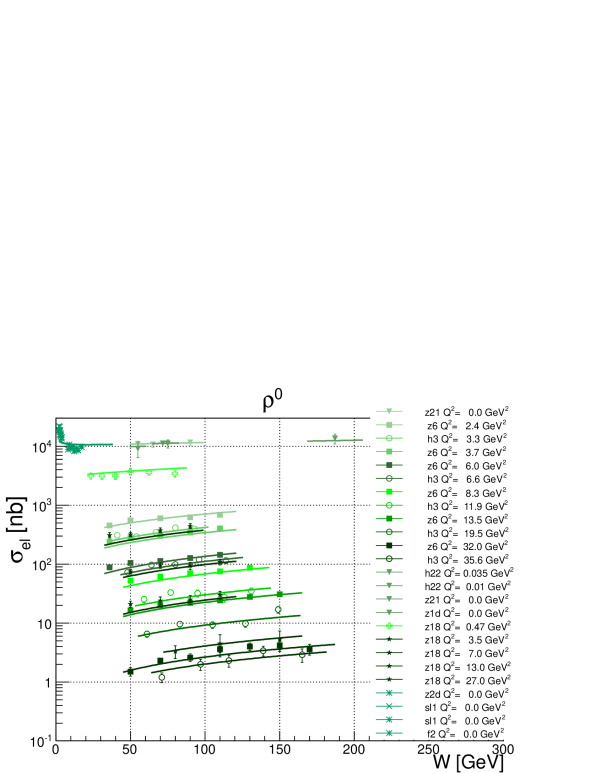
Figure 9: Fit of Equation (60) to data on elastic cross section $\sigma_{el}(W)$ for $\rho^{0}$, for different values of $Q^{2}$.

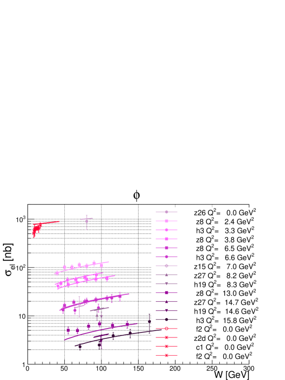
Figure 10: Fit of Equation (60) to the data on elastic cross section $\sigma_{el}(W)$ for $\phi$, for different values of $Q^{2}$.

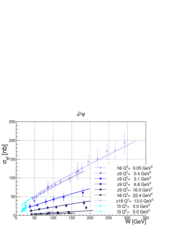
Figure 11: Fit of Equation (60) to the data on elastic cross section $\sigma_{el}(W)$ for $J/\psi$, for different values of $Q^{2}$.

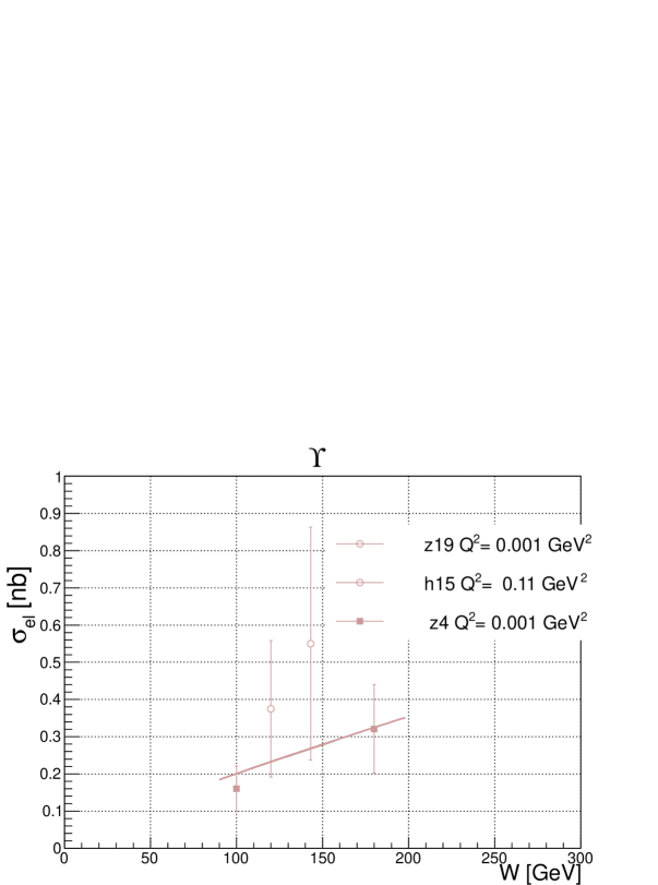
Figure 12: Fit of Equation (60) to the data on elastic cross section $\sigma_{el}(W)$ for $\varUpsilon$, for different values of $Q^{2}$.

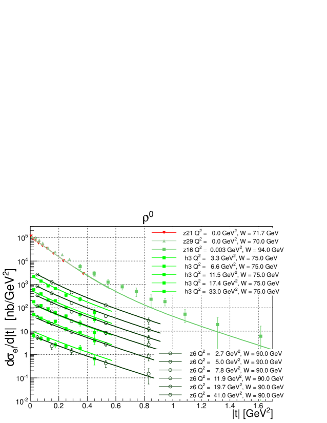
Figure 13: Fit of Equation (59) to the data on the differential elastic cross section $d\sigma_{el}/dt$ for $\rho^{0}$, for different values of $Q^{2}$ and $W$.

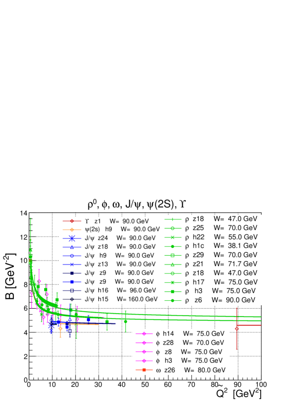
Figure 14: Experimental data on the slope $B$ as function of $\widetilde{Q^{2}}$ for $\rho^{0},\phi,J/\psi$, $\varUpsilon$ and $\Psi$(2S), and our theoretical predictions from Equation (63).

Table 2: Parameters of the two-component pomeron model (Equations (59) and (60)) fitted to the combined VMP and DVCS data, with fixed parameters of the pomeron trajectories $\alpha_{s}(t)=1.08+0.25t$ and $\alpha_{h}(t)=1.20+0.01t$.

	$A_{0s,h}$ $\left[\frac{\sqrt{\text{{nb}}}}{\text{{GeV}}}\right]$	$\widetilde{Q^{2}_{s,h}}$ $\left[\text{{GeV}}^{\textbf{2}}\right]$	$n_{s,h}$	$\alpha_{0\,s,h}$	$\alpha^{\prime}_{s,h}$ $\left[\frac{\textbf{1}}{\text{{GeV}}^{\textbf{2}}}\right]$	$b_{s,h}$ $\left[\frac{\textbf{1}}{\text{{GeV}}^{\textbf{2}}}\right]$
soft	807 $\pm$ 1107	0.46 $\pm$ 0.70	1.79 $\pm$ 0.79	1.08	0.25	3.41 $\pm$ 2.48
hard	47.9 $\pm$ 46.9	1.30 $\pm$ 1.12	1.33 $\pm$ 0.26	1.20	0.01	2.15 $\pm$ 1.14

More results and discussion on the fitting details can be found in Refs. Salii1 ; Salii2 .

VI Balancing between “Soft” and “Hard” Dynamics

In this section we illustrate the important and delicate interplay between the “soft” and “hard” components of our unique pomeron. Since the amplitude consists of two parts, according to the definition  (50), it can be written as

$$A(Q^{2},s,t)=A_{s}(Q^{2},s,t)+A_{h}(Q^{2},s,t).$$ (64)

As a consequence, the differential and elastic cross sections contain also an interference term between “soft” and “hard” parts, so that they read

$$\frac{d\sigma_{el}}{dt}=\frac{d\sigma_{s,el}}{dt}+\frac{d\sigma_{h,el}}{dt}+\frac{d\sigma_{interf,el}}{dt}$$ (65)

and

$$\sigma_{el}=\sigma_{s,el}+\sigma_{h,el}+\sigma_{interf,el},$$ (66)

according to Equations (59) and (60), respectively.

Given Equations (65) and (66), we can define the following ratios for each component:

$$R_{i}(\widetilde{Q^{2}},W,t)=\frac{\frac{d\sigma_{i,el}}{dt}}{\frac{d\sigma_{el}}{dt}}$$ (67)

and

$$R_{i}(\widetilde{Q^{2}},W)=\frac{\sigma_{i,el}}{\sigma_{el}},$$ (68)

where $i$ stands for $\{s,h,interf\}$.

Figure 15 shows the interplay between the components for both $\sigma_{i,el}$ and $R_{i}(\widetilde{Q^{2}},t)$, as functions of $\widetilde{Q^{2}}$, for $W$ = 70 GeV. In Figure 16 both plots show that not only $\widetilde{Q^{2}}$ is the parameter defining softness or hardness of the process, but such is also the combination of $\widetilde{Q^{2}}$ and $t$, similar to the variable $z=t-Q^{2}$ introduced in Ref. Capua . On the whole, it can be seen from the plots that the soft component dominates in the region of low $\widetilde{Q^{2}}$ and low $|t|$, while the hard component dominates high $\widetilde{Q^{2}}$ and high $|t|$.

In other words, the variables $t$ and $Q^{2}$ have much in common: both refer to squared momentum transfer and have the meaning of “hardness”. The present model provides a valuable laboratory to study this important issue.

Hadron-induced reactions, discussed in Section II differ from those induced by photons at least in two aspects. First, hadrons are on the mass shell and hence the relevant processes are typically “soft”. Secondly, the mass of incoming hadrons is positive, while the virtual photon has negative squared “mass”. Our attempt to include hadron-hadron scattering into the analysis with our model has the following motivations: (a) by vector meson dominance (VMD) the photon behaves partly as a meson, therefore meson–baryon (and more generally, hadron-hadron) scattering has much in common with photon-induced reactions. Deviations from VMD may be accounted for the proper $Q^{2}$ dependence of the amplitude (as we do hope is in our case!); (b) connection between space- and time-like reactions; (c) according to some claims the highest-energy (LHC) proton–proton scattering data indicate the need for a “hard” component in the pomeron (to anticipate, our fits do not found support the need of any noticeable “hard” component in $pp$ scattering).

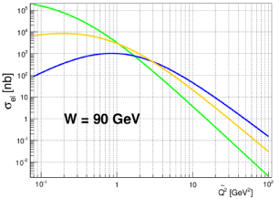
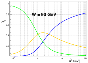
Figure 15: Interplay between soft (green line), hard (blue line) and interference (yellow line) components of the cross section $\sigma_{i,el}$ (left plot) and $R_{i}(\widetilde{Q^{2}},t)$ (right plot) as functions of $\widetilde{Q^{2}}$, for $W=70$ GeV.

We do not intend to perform here a high-quality fit to the $pp$ data; that would be impossible without the inclusion of subleading contributions and/or the odderon.

The $pp$ scattering amplitude is written in the form similar to the amplitude (58) for VMP or DVCS, the only difference being that the normalization factor is constant since the $pp$ scattering amplitude does not depend on $Q^{2}$:

$$A^{pp}(s,t)=A^{pp}_{s}\,e^{-i\frac{\pi}{2}\alpha_{s}(t)}\left(\frac{s}{s_{0}}\right)^{\alpha_{s}(t)}e^{b_{s}t}+A^{pp}_{h}\,e^{-i\frac{\pi}{2}\alpha_{h}(t)}\left(\frac{s}{s_{0}}\right)^{\alpha_{h}(t)}e^{b_{h}t}.$$ (69)

We fix the parameters of pomeron trajectory at

$$\alpha_{s}(t)=1.084+0.35t,\qquad\alpha_{h}(t)=1.30+0.10t.$$

With these trajectories the total cross section

$$\sigma_{tot}=\frac{4\pi}{s}Im\;A(s,{t=0})$$ (70)

was found compatible with the LHC data. From the comparison of Equation (70) to the LHC data we get

$$A^{pp}_{s}=-1.73\text{\,mb}\cdot\text{GeV}^{2},\,\,\quad\quad A^{pp}_{h}=-0.0012\text{\,mb}\cdot\text{GeV}^{2}.$$

We conclude that, while the data on total cross section are compatible with a small “hard” admixture in the amplitude, the slope parameter with a hard component included seems to manifest a wrong tendency, by slowing down with increasing energy, while the TOTEM measurements show the opposite.

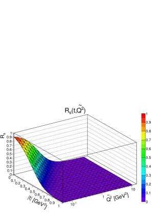
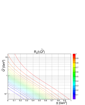
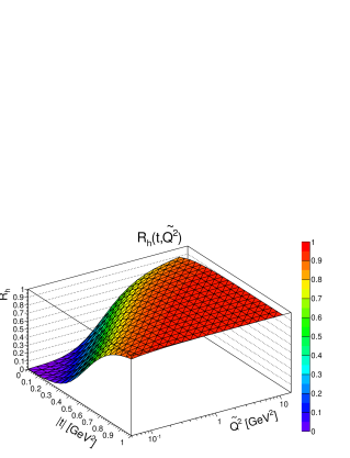
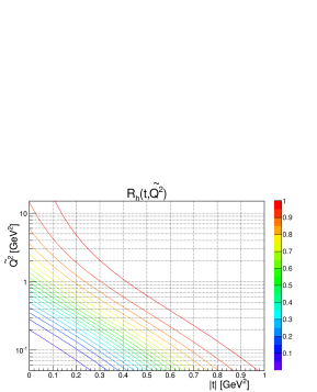
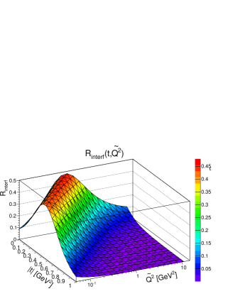
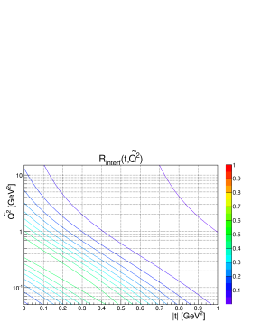
Figure 16: Left column: soft (upper surface), hard (middle surface) and interference (bottom surface) components of the ratio $R_{i}(\widetilde{Q^{2}},W,t)$ are shown as functions of $\widetilde{Q^{2}}$ and $t$, for $W=70$ GeV. Right column: some representative curves of the surfaces projected on the ($t,\widetilde{Q^{2}}$ ) plane.

The resulting fits are reasonable, despite the following open problems:

• sub-leading Regge contributions must be included in any extension of the model to lower energies (below $30$ GeV);

• the $\widetilde{Q^{2}}$ dependence of the scattering amplitude, introduced empirically has to be compared with the results of unitarization and/or QCD evolution.

• as seen from Section VI, the “soft” component of the pomeron dominates in the region of small $t$ and small $\widetilde{Q^{2}}$. Hence, any parameter responsible for the “softness” and/or “hardness” of processes, should be a combination of $t$ and $Q^{2}$. A simple solution was suggested in Ref. Capua with the introduction of the variable $z=t-Q^{2}$. The interplay of these two variables remains an important open problem that requires further investigation.

The extension of our formalism to hadronic reactions ($pp$ scattering) shows that the available data can be will described by a single—soft—component.

VII Spin of the Proton in Terms of Its Constituents

The origin of spin in the nucleon is a rich subject deserving a dedicated presentation. Here I only briefly sketch some recent developments in the field. A complete and comprehensive treatment of the subject can be found e.g., in Refs. Leader0 ; Rev2 .

In the simplest case, if only valence quarks contributed, the nucleon spin would be simple a sum

$$J=\frac{\Delta\Sigma}{2}+L_{q}=\frac{1}{2},$$ (71)

where $\Delta\Sigma$ is the quark spin contribution and $L_{q}$ is the orbital angular momentum (OAM) contribution. Partition between the quark spin and the OAM for a long time were subject of debates generally called “spin crisis”. Estimates of shares varied in a wide range. Among the reasons of disagreement and contradictions was the role of gluons, and sea as compared to that of the valence quarks. The phenomenon known as “spin crisis” arose from an EMC experiment at CERN EMC quoting $\Sigma\approx 0$ (with large uncertainty), thus allegedly contradicting the naive quark model. Recent COMPAS, HERMES and Jlab measurements are consistent with a value of $\Sigma\approx 0.3.$ Actually, $J$ must obey conservation of the total angular momentum known as Jaffe-Manohar sum rule Jaffe_Manohar ,

$$J=\Delta\Sigma(Q^{2})+L_{q}(Q^{2})+\Delta(Q^{2})+L_{q}(Q^{2})=\frac{1}{2}.$$ (72)

An important task in the context of the above some rule is the separation of sea and valence quarks, indistinguishable in DIS observables. In addition, as  noted in Ref. BMa , strange and anti-strange sea quarks can contribute differently in to the nucleon spin.

Paper Rev2 discusses also how DIS data on proton, neutron and deuteron targets can be used to separate the contributions from different quark polarizations assuming validity of $SU(3)_{f}$.

That paper contains many more ideas, among which is the use of parton–hadron duality of Bloom and Gilman B-G —another effective tool to be used in studies of spin effects and a possible key to understand better problems related to quark confinement.

Before the advent of QCD, a nucleon (N) was visualized as a bound state of 3 massive quarks (Q) ( $M_{Q}\approx M_{N}/3$) lying in some kind of potential. In the simplest non-relativistic case, for an s-state the constituent quarks have no orbital angular momentum (OAM) and one has, for the nucleon at rest, say polarized in the positive Z-direction

$$1/2=S_{z}^{N}=\sum_{Q}S_{z}^{Q}.$$ (73)

With relativistic corrections, the bottom components of the quark Dirac spinors contain OAM and Equation (73) is modified to

$$\sum_{Q}S_{z}^{Q}\approx 0.3$$ (74)

In the naive parton model, for a fast moving proton with helicity $+1/2$,

$$a_{0}=\Delta\Sigma\equiv(\Delta u+\Delta\overline{u})+(\Delta d+\Delta\overline{d})+(\Delta s+\Delta\overline{s})$$ (75)

where the $\Delta q$, $\Delta\bar{q}$ are the first moments of the polarized quark–parton helicity densities. Hence, bearing in mind that $\Delta q=q_{+}-q_{-}$, where $\pm$ corresponds to the number densities with spin along or opposite to the proton’s momentum, one obtains in the naive parton model

$$a_{0}=\Delta\Sigma=2\left[\sum_{q}\langle S_{z}^{q}\rangle+\sum_{\bar{q}}\langle S_{z}^{\bar{q}}\rangle\right]$$ (76)

and if there is no other source of angular momentum one expects

$$\left[\sum_{q}\langle S_{z}^{q}\rangle+\sum_{\bar{q}}\langle S_{z}^{\bar{q}}\rangle\right]=S_{z}^{\textrm{proton}}=1/2$$ (77)

implying, naively,

$$a_{0}=1.$$

After the famous EMC experiments revealed that only a small fraction of the nucleon spin is due to quark spins, there has been great interest in ‘solving the spin puzzle’, i.e., in decomposing the nucleon spin into contributions from quark/gluon spin and orbital degrees of freedom.

The EMC experiment gave $a_{0}\approx 0$ and later experiments confirmed that $a_{0}\ll 1$, giving rise to the spin crisis in the (naive) parton model. However, Equation (VII) cannot possibly be true because the right hand side is a fixed number, whereas the left hand side is, beyond the naive level, equal to $a_{0}(Q^{2})$, i.e., a function of $Q^{2}$! Thus failure of Equation (VII) to hold cannot be used to infer that there is crisis. It is obvious that a correct relation between the spin of a nucleon and the angular momentum of its constituents should include their orbital angular momentum and should also include a contribution from the gluons.

Ji’s and J-M’s Decompositions

Finally, we briefly mention two sum rules visualising in different albeit complementary ways the spin decomposition in the nucleon.

The Ji decomposition Ji:1996ek

$$\frac{1}{2}=\frac{1}{2}\sum_{q}\Delta q+\sum_{q}{L}_{q}^{z}+J_{g}^{z}$$ (78)

appears to be very useful, as not only the quark spin contributions $\Delta q$ but also the quark total angular momenta $J_{q}\equiv\frac{1}{2}\Delta q+{L}_{q}^{z}$ (and by subtracting the spin piece also the the quark orbital angular momenta $L_{q}^{z}$) entering this decomposition can be accessed experimentally, through generalized parton distributions (GPDs). The terms in (78) are defined as expectation values of the corresponding terms in the angular momentum tensor

$$M^{0xy}=\sum_{q}\frac{1}{2}q^{\dagger}\Sigma^{z}q+\sum_{q}q^{\dagger}\left({\vec{r}}\times i{\vec{D}}\right)^{z}q+\left[{\vec{r}}\times\left({\vec{E}}\times{\vec{B}}\right)\right]^{z}$$ (79)

in a nucleon state with zero momentum. Here $i{\vec{D}}=i{\vec{\partial}}-g{\vec{A}}$ is the gauge-covariant derivative.

Jaffe and Manohar proposed Jaffe_Manohar an alternative decomposition of the nucleon spin, which does have a partonic interpretation

$$\frac{1}{2}=\frac{1}{2}\sum_{q}\Delta q+\sum_{q}{\cal L}_{q}^{z}+\frac{1}{2}\Delta G+{\cal L}_{g}^{z},$$ (80)

whose terms are defined as matrix elements of the corresponding terms in the $+12$ component of the angular momentum tensor

$$M^{+12}=\frac{1}{2}\sum_{q}q^{\dagger}_{+}\gamma_{5}q_{+}+\sum_{q}q^{\dagger}_{+}\left({\vec{r}}\times i{\vec{\partial}}\right)^{z}q_{+}+\varepsilon^{+-ij}\mbox{Tr}F^{+i}A^{j}+2\mbox{Tr}F^{+j}\left({\vec{r}}\times i{\vec{\partial}}\right)^{z}A^{j}.$$ (81)

In Figure 17 the share of various components to the nucleon spin, according to the two (Ji and Jaffe-Manohar) distribtutions is shown.

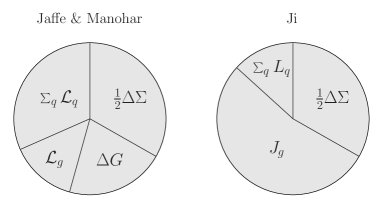
Figure 17: Origin of the proton spin according to sum rules of Jaffe, and Monahor and Ji.

What appeared to be spin crisis in the parton model, over three decades years ago, was a consequence of a misinterpretation of the results of the famous European Muon Collaboration experiment on polarized deep inelastic scattering.

VIII Conclusions

Interest in spin physics and polarization has moved from hadron-hadron to lepton-hadron processes. This is mainly due to the fact that in proton–proton and proton–antiproton scattering spectacular spin effects were/are not expected at highest energies (ISR, Fermilab, BNL or LHC), except maybe for the dip-bump structure at the diffraction cone. Various aspects of polarization in inelastic hadronic reactions reactions were treated in simple intuitive models in Refs. Strum .

Instead, deeply virtual Compton scattering (DVCS), with spin degrees of freedom is now at the focus of interest as a source of information on generalized parton distributions (GPDs).

In both cases (hadron-hadron and lepton-hadron) diffraction and the pomeron play a crucial role. Therefore much space was dedicated to the theoretical problems of diffractive scattering, properties of the vacuum Regge trajectory (pomeron), and confinement of quarks and gluons.

In the near future, research programs at the Electron-Ion Colliders (EICs) will play an important role in understanding gluon GPDs. Apart from providing constraints on the total quark/gluon contributions to the proton spin, the GPD’s will provide important information on the nucleon tomography, for example, the 3D imaging of partons inside the proton. Together with the gravitational form factors extracted from the DVCS, this will deepen our understanding of the nucleon spin structure in return. The EIC may shed light on the quark/gluon orbital angular momentum (OAM) directly through various hard diffractive processes. Pioneer experimental effort to constrain the gravitation form factor from DVCS experiment at JLab has been carried out in Ref. Grav . The quark and gluon helicity contributions to the proton spin with the unique coverage in both $x$ and $Q^{2}$ at EIC will provide the most stringent constraints on $\Delta\Sigma$ and $\Delta G$ EIC1 ; EIC2 .

Last but not least, Regge trajectories Section II.2, relating uniquely the spin and mass of particles, are building blocks of the theory, containing the basic information on the dynamics. By crossing symmetry, unitarity and duality they relate various aspects of high-energy strong interaction dynamics.

This research received no external funding

- (1) Ashman, J. European Muon Collaboration. Phys. Lett. B 1988, 206, 364. [CrossRef]
- (2) Deur, A.; Brodsky, S.J.; De Teramond, G.F. The Spin Structure of the Nucleon. Rept. Prog. Phys. 2019, 82. [CrossRef]
- (3) Volker Burkert, L.; Elouadrhihiri, F.X. Girod. Nature 2018, 557, 396–399.
- (4) Gibson, A.; Stanisalus, S.; Koetke, D.D.; STAR Collaboration. Global Lambda hyperon polarization in nuclear collisions: Evidence for the most vortical fluid. Nature 2017, 548, 62–65. [CrossRef]
- (5) Becattini, F.; Chandra, V.; Del Zanna, L.; Grossi, E. Relativistic distribution function for particles with spin at local thermodynamical equilibrium. Ann. Phys. 2013, 338, 32–49. [CrossRef]
- (6) Karpenko, I.; Becattini, F. Study of polarization in relativistic nuclear collisions at –200 GeV. Eur. Phys. J. 2017, C77, 213. [CrossRef]
- (7) Xie, Y.; Wang, D.; Csernai, L.P. Global polarization in high energy collisions. Phys. Rev. 2017, C95, 031901. [CrossRef]
- (8) Cane, G.L.; Pumplin, J.; Repko, W. Transverse Quark Polarization a Test of Quantum Chromodynsmics. Phys. Rev. Lett. 1978, 41, 1689–1692.
- (9) Struminsky, B.V. Quark Dynamics of Polarization Phenomena in Inclusive Processes. Sov. J. Nucl. Phys. 1981, 34, 885.
- (10) Kuhn, S.E.; Chen, J.-P.; Leader, E. Spin Structure of the Nucleon—Status and Recent Results. Prog. Part Nucl. Phys. 2009, 63, 1–50. [CrossRef]
- (11) Aidala, C.A.; Bass, S.D.; Hasch, D.; Mallot, G.K. The Spin Structure of the Nucleon. Rev. Mod. Phys. 2013, 85, 655–691. [CrossRef]
- (12) Biró, T.; Schramm, Z.; Jenkovszky, L. Entropy Production During Hadronization of a Quark-Gluon Plasma. Eur. Phys. J. A 2018, 54, 17. [CrossRef]
- (13) Vall, A.N.; Jenkovszky, L.L.; Struminsky, B.V. High-Energy Hadron Interactions. Sov. J. Part. Nucl. 1988, 19, 1.
- (14) Bystricky, J.; Lehar, F.; Winternitz, P. Formalism Of Nucleon-Nucleon Elastic Scattering Experiments. J. Phys. 1978, 39, 1. [CrossRef]
- (15) Lechanoine-LeLuc, C.; Lehar, F. Nucleon-nucleon elastic scattering and total cross-sections. Rev. Mod. Phys. 1993, 65, 47. [CrossRef]
- (16) Troshin, S.M.; Tyurin, N.E. Spin Phenomena in Particle Interactions; World Scientific: Singapore, 1994; p. 211.
- (17) Edneral, V.F.; Troshin, S.M.; Tyurin, N.E. On Spin Effects in Elastic Scattering at Large Momentum Transfers. JETP Lett. 1979, 30, 330.
- (18) Cudell, J.-R.; Selyugin, O.V. The spin-flip amplitude in the impact-parameter representation. arXiv 2008, arXiv:0812.4371.
- (19) Selyugin, V. High Energy Hadron Spin Flip Amplitude. arXiv 2016, arXiv:1512.05130.
- (20) Capella, A.; Contogouris, A.P.; Van, J.T. Factorization and constraints in Regge pole theory. Phys. Rev. 1968, 175, 1892. [CrossRef]
- (21) Szanyi, I.; Jenkovszky, L.; Schicker, R.; Svintozelskyi, V. Pomeron/glueball and odderon/oddball trajectories. Nucl. Phys. A 2020, 998, 121728. [CrossRef]
- (22) Jenkovszky, L.; Schicker, R.; Szanyi, I. Elastic and diffractive scattering in the LHC era. Int. J. Mod. Phys. E 2018, 27, 1830005. [CrossRef]
- (23) Jenkovszky, L.L.; Paccanoni, F. Impact parameter Analysis of DAMA. Nouvo Cim. 1976, 33A, 329.
- (24) Troshin, S.M.; Tyurin, N.E. The Emergent Black Ring. Mod. Phys. Lett. A 2019, 33, 1950259. [CrossRef]
- (25) Phillips, R.J.N. A Dipole Pomeron Ansatz; PL-74-03 Preprint; Rutherford Lab.: Chilton, UK, 1974.
- (26) Jenkovszky, L.L. Phenomenology of Elactic Hadron Scattering. Fortschritte Der Phys. 1986, 34, 701.
- (27) Müller, D.; Robaschik, D.; Geyer, B.; Dittes, F.-M.; Hořejši, J. Wave Functions, Evolution Equations and Evolution Kernels from Light-Ray Operators of QCD. Fortschr. Phys. 1994, 42, 101. [CrossRef]
- (28) Radyushkin, A.V. Scaling Limit of Deeply Virtual Compton Scattering. Phys. Lett. 1996, B380, 41. [CrossRef]
- (29) Ji, X. Deeply Virtual Compton Scattering. Phys. Rev. 1997, D55, 7114. [CrossRef]
- (30) Collins, J.; Frankfurt, L.; Strikman, M. Factorization for Hard Exclusive Electroproduction of Mesons in QCD. Phys. Rev. 1997, D56, 2982.
- (31) Collins, J.; Freund, A. Proof of Factorization for Deeply Virtual Compton Scattering in QCD. Phys. Rev. 1999, D59, 074009. [CrossRef]
- (32) Diehl, M.; Feldmann, T.; Jakob, R.; Kroll, P. Linking parton distributions to form factors and Compton scattering. Eur. Phys. J. 1999, C8, 409. [CrossRef]
- (33) Diehl, M.; Feldmann, T.; Jakob, R.; Kroll, P. The Overlap Representation of Skewed Quark and Gluon Distributions. Nucl. Phys. 2001, B596, 33. [CrossRef]
- (34) Diehl, M. Generalized Parton Distributions. Phys. Rep. 2003, 388, 41. [CrossRef]
- (35) Belitsky, A.V.; Radyushkin, A.V. Unraveling Hadron Structure with Generalized Parton Distributions. Phys. Rep. 2005, 418, 1. [CrossRef]
- (36) Burkardt, M. Off-Forward Parton Distributions in 1+1 Dimensional QCD. Phys. Rev. 2000, D62, 071503.
- (37) Diehl, M. Generalized parton distributions in impact parameter space. Eur. Phys. J. 2002, C25, 223. [CrossRef]
- (38) Kogut, J.; Soper, D. Quantum Electrodynamics in the Infinite-Momentum Frame. Phys. Rev. 1970, D1, 2901.
- (39) Ji, X. Gauge-Invariant Decomposition of Nucleon Spin and Its Spin-Off. Phys. Rev. Lett. 1997, 78, 610. [CrossRef]
- (40) Aschenauer, E.-C.; Fazio, S.; Kumericki, K.; Mueller, D. Deeply Virtual Compton Scattering at a Proposed High-Luminosity Electron-Ion Collider. arXiv 2013, arXiv:1304.0077.
- (41) Accardi, A.; Albacete, J.L.; Anselmino, M.; Armesto, N.; Aschenauer, E.C.; Bacchetta, A.; Boer, D.; Brooks, W.; Burton,T.; Chang, N.-B.; et al. Electron Ion Collider: The Next QCD Frontier - Understanding the glue that binds us all. arXiv 2012, arXiv:1212.1701
- (42) Ji, X.-D. Off-Forward Parton Distributions. J. Phys. G 1998, 24, 1181. [CrossRef]
- (43) Belitsky, A.V.; Müller, D.; Kirchner, A. Theory of Deeply Virtual Compton Scattering on the Nucleon. Nucl. Phys. 2002, B629, 323. [CrossRef]
- (44) Capua, M.; Fiore, R.; Jenkovszky, L.; Paccanoni, F. A Deeply Virtual Compton Scattering Amplitude. Phys. Lett. 2007, B645, 161. [CrossRef]
- (45) Fazio, S.; Fiore, R.; Lavorini, A.; Jenkovszky, L.; Salii, A. Reggeometry of Deeply Virtual Compton Scattering (DVCS) and Exclusive Vector Veson Production (VMP) at HERA. Acta Phys. Polonica B 2013, 44, 1333. [CrossRef]
- (46) Fazio, S.; Fiore, R.; Jenkovszky,L.; Salii, A. Unifying “Soft” and “Hard” Diffractive Exclusive Vector Meson Production and Deeply Virtual Compton Scattering. Phys. Rev. D 2014, 90, 016007-1.
- (47) Donnachie, A.; Landshoff, P. Elastic Scattering and Diffraction Dissociation. Nucl. Phys. 1984, B231, 189.
- (48) Donnachie, A.; Landshoff, P.V. Small x: Two Pomerons! Phys. Lett. 1998, B437, 408. [CrossRef]
- (49) Jaffe, R.L.; Manohar, A. The g1 Problem: Deep Inelastic Electron Scattering and the Spin of the Proton. Nucl. Phys. 1990, 337, 509. [CrossRef]
- (50) Brodsky, S.J.; Ma, B.Q. The Quark/Antiquark Asymmetry of the Nucleon Sea. Phys. Lett. B 1996, 381, 317. [CrossRef]
- (51) Bloom, E.D.; Gilman, F.J. Scaling, Duality, and the Behavior of Resonances in Inelastic Electron-Proton Scattering. Phys. Rev. Lett. 1970, 25, 1140. [CrossRef]
- (52) Ji, X.; Yuan, F.; Zhao, Y. Proton spin after 30 years: What we know and what we don’t? arXiv 2009, arXiv:2009.01291.
- (53) Accardi, A.; Albacete, J.L.; Anselmino, M.; Armesto, N.; Aschenauer, E.C.; Bacchetta, A.; Deng, W.T. Electron Ion Collider: The Next QCD Frontier. Eur. Phys. J. A 2016, 52, 268.