Iterative Surface Mapping Using Local Geometry Approximation with Sparse Measurements During Robotic Tooling Tasks

Abstract

We present a cost-efficient and versatile method to map an unknown 3D freeform surface using only sparse measurements while the end-effector of a robotic manipulator moves along the surface. The geometry is locally approximated by a plane, which is defined by measured points on the surface. The method relies on linear Kalman filters, estimating the height of each point on a 2D grid. Therefore, the approximation covariance for each grid point is determined using a radial basis function to consider the measured point positions. We propose different update strategies for the grid points exploiting the locality of the planar approximation in combination with a projection method. The approach is experimentally validated by tracking the surface with a robotic manipulator. Three laser distance sensors mounted on the end-effector continuously measure points on the surface during the motion to determine the approximation plane. It is shown that the surface geometry can be mapped reasonably accurate with a mean absolute error below 1 mm. The mapping error mainly depends on the size of the approximation area and the curvature of the surface.

0.87(0.06,0.93) ©2021 IEEE. Personal use of this material is permitted. Permission from IEEE must be obtained for all other uses, in any current or future media, including reprinting/republishing this material for advertising or promotional purposes, creating new collective works, for resale or redistribution to servers or lists, or reuse of any copyrighted component of this work in other works.

I INTRODUCTION

The knowledge of the exact geometry of a part is crucial for most automated manufacturing techniques like milling, polishing or grinding. In usual production scenarios, the geometry is determined by CAD drawings. But in cases where this data is not available, it has to be reconstructed by using highly accurate coordinate measuring machines (CMM) [1] or vision-based techniques such as structured light sensing [2, 3, 4]. However, these techniques are expensive, require exhaustive calibration and can only map a limited volume. For the machining of large parts or mobile manufacturing scenarios, this may be inappropriate. Especially in small and medium-sized enterprises with high-mix low-volume production, the required large investments for measurement equipment might become an obstacle for the automation of manufacturing processes. Therefore, it is our aim in this contribution to develop a versatile and cost-efficient method to map an unknown geometry focusing on robotic tooling tasks. The resulting 3D model provides the basis to improve the path and motion planning of the process.

The work presented in [5] uses local parameterized patches from sparse depth measurements to reconstruct a surface on a dense 2D grid. Therefore, polynomial surface patches are determined such that the maximum approximation error is minimized. In [6], a 6-DOF robotic manipulator moves a part in front of a stationary 2D laser scanner. The scanned points are combined with the robot’s forward kinematics to reconstruct the geometry of the part. This limits the approach to applications, where the part is small enough to be moved by the robot. The geometry of the surface can also be determined during force-controlled interaction between tool and surface, assuming a known contact point, as demonstrated in [7]. However, this gives only the contour along the performed path but not in its vicinity. A similar approach is used in [8] with an impedance controller to iteratively update an estimate of the surface geometry. This requires an initial coarse sampling of the surface, which is represented as bi-linear interpolation of the sampling points. Other tactile approaches, such as those proposed in [9, 10], require geometric primitives to identify the shape parameters from sparse measurement points. In [11], planar patches, obtained from sparse point clouds, are used to reconstruct a large-scale surface. These planar patches serve as features in a real-time SLAM implementation. A similar approach is used in [12] for visual mapping. Kalman filter-based methods are widely used for SLAM but can also be exploited for map data fusion [13]. A probabilistic representation of an object model is proposed in [14], where better explored regions have a higher probability.

This paper presents a novel method to map the surface geometry using sparse sensor measurements to approximate the surface locally. The sensors are mounted on a robotic manipulator that moves along the surface. During this motion, the mapping is continuously updated by these approximations. In this way, a large area can be covered. Another advantage of the robotic setup is that hidden parts can be mapped, which would not be visible to stationary 3D scanners and the part is scanned from different directions without requiring a rotary table. By weighting the updates based on a radial basis function (RBF) as a heuristical estimate of the approximation covariance, the mapping is iteratively improved. Different region-based update schemes, implemented by binary masks, allow us to update the mapping only in regions where the approximation is valid. The approach is evaluated on an experimental setup. The measurement works with laser distance sensors but can also be used with other distance sensor types, e.g., tactile, inductive or capacitive, to measure even materials which might be hard to detect with optical sensors, such as transparent, reflective or dark surfaces. Therefore, the approach provides an alternative solution to commercial 3D scanning methods for applications where not their full $\mathrm{\SIUnitSymbolMicro m}$-accuracy is required.

The paper is structured as follows: First, the representation and the local approximation of the surface are described in Section II. The mapping method is then introduced in Section III by defining the Kalman filters for height estimation, the measurement covariance and some mask types for the local update. Section IV describes the experimental setup, which is used for the mapping of the example surface. The results are presented and discussed in Section V. Section VI concludes the paper and gives some ideas for future work.

II SURFACE APPROXIMATION

Figure 1: Local approximation of the freeform surface (grey) as a plane (orange) determined from three measured points (red) and coordinate frames $\{0\}$ (black) and $\{A\}$ (blue).

The proposed approach relies on the fact that the surface can be approximated locally by a geometric primitive such as a plane. In this section, we first define a mathematical representation of the surface, which is used for the later mapping. Afterwards, the local approximation of the geometry is described using sparse measurement points on the surface.

II-A Surface Representation

To represent the surface geometry, we define the surface as a height map on a 2D grid. Without loss of generality, the grid is given inside a rectangular area in the $xy$-plane of the inertial coordinate system $\{0\}$. Therefore, the $x$- and $y$-coordinates are discretized in the intervals $x\in[x_{\text{min}},\,x_{\text{max}}]$ and $y\in[y_{\text{min}},\,y_{\text{max}}]$. The geometry of the surface is determined by its height

$$\bar{z}_{ij} =f(x_{i},\,y_{j})$$ (1a)

on each grid point

$$x_{i} =h_{x}i+x_{\text{min}}\quad i=0,\,\ldots,\,N-1$$ (1b)

$$y_{j} =h_{y}j+y_{\text{min}}\quad j=0,\,\ldots,\,M-1,$$ (1c)

where the values $h_{x}=\frac{x_{\text{max}}-x_{\text{min}}}{N}$ and $h_{y}=\frac{y_{\text{max}}-y_{\text{min}}}{M}$ denote the step size of the grid in $x$- and $y$-direction. The mapping $f:\mathbb{R}^{2}\rightarrow\mathbb{R}$ is assumed to be unique over the grid. Using an affine transformation ${\boldsymbol{p}}^{\prime}=(R_{0}^{\text{A}})^{\textrm{\scriptsize{T}}}({\boldsymbol{p}}-{\boldsymbol{p}}_{0}^{\text{A}})$ allows us to transform the desired part of the surface such that it can be parameterized by the $xy$-plane of the local coordinate system $\{\text{A}\}$, where $R_{0}^{\text{A}}\in\mathrm{SO}(3)$ denotes the rotation matrix and ${\boldsymbol{p}}_{0}^{\text{A}}\in\mathbb{R}^{3}$ the origin of the local coordinate system with respect to the inertial coordinate system.

II-B Local Geometry Approximation

As described in [15], the surface geometry can be approximated using sparse measurements of points on the surface. In Fig. 1, the local approximation of the surface is shown. Three measurement points are used to define a plane, which approximates the surface geometry locally. This provides a first-order approximation of the local geometry, which can be expressed by the surface normal vector ${\boldsymbol{n}}=[n_{x}\>n_{y}\>n_{z}]^{\textrm{\scriptsize{T}}}$ and the distance $p$ of the plane from the origin. For $L\geq 3$ distinct measurement points ${\boldsymbol{p}}_{1},\,\ldots,\,{\boldsymbol{p}}_{L}\in\mathbb{R}^{3}$, the surface normal vector ${\boldsymbol{n}}$ can be determined as the eigenvector corresponding to the smallest eigenvalue of the covariance matrix

$$C=\frac{1}{L}\sum_{l=1}^{L}({\boldsymbol{p}}_{l}-{\boldsymbol{p}}_{c})({\boldsymbol{p}}_{l}-{\boldsymbol{p}}_{c})^{\textrm{\scriptsize{T}}}\;\;\text{with}\;{\boldsymbol{p}}_{c}=\frac{1}{L}\sum_{l=1}^{L}{\boldsymbol{p}}_{l},$$ (2)

where ${\boldsymbol{p}}_{c}$ is the centroid of all points. This method is also known as principal component analysis (PCA) for point clouds [16, 17]. The distance $p$ of the plane from the origin then follows as $p={\boldsymbol{n}}\cdot{\boldsymbol{p}}_{c}$, assuming that the plane goes through the center point ${\boldsymbol{p}}_{c}$. For $L=3$, all three measurement points and the center point lie on the plane. The length of the normal vector equals to $\|{\boldsymbol{n}}\|=1$ per definition. The $z$-coordinate of the points on the approximation plane ${\boldsymbol{p}}_{0}^{S}(x_{i},\,y_{j})=[x_{i}\>y_{j}\>z_{ij}]^{\textrm{\scriptsize{T}}}$ is obtained as

$$z_{ij}=\frac{1}{n_{z}}(p-n_{x}x_{i}-n_{y}y_{j})$$ (3)

for a given $x_{i}$ and $y_{j}$ value, assuming $n_{z}\neq 0$.

Notice that the approximation plane may intersect the surface depending on the alignment of the measurement points. According to the mean value theorem, this plane also approximates the tangential plane of the surface. In a sufficiently small area, the error between the surface geometry and the approximation function is bounded. This only holds as long as the curvature in this area is sufficiently small, which is valid when the curvature radius is much larger than the distance between the measurement points. In this paper, it is assumed that the surface is approximated on a subset of the grid points inside the approximation area $\mathcal{A}\subset\mathbb{R}^{2}$. Let $\mathcal{I}:=\{(i,\,j)|(x_{i},\,y_{j})\in\mathcal{A},\,\forall\,(i,\,j)\in\{1,\,\ldots,\,M\}\times\{1,\,\ldots,\,N\}\}$ be the set of indices for all grid points inside this area. The definition of such a local approximation area is discussed in Section III-C.

To project coordinates from the inertial coordinate system $\{0\}$ onto the plane, we define a local coordinate frame $\{\text{A}\}$ on the plane. The approximation center point is chosen as the origin of the frame ${\boldsymbol{p}}_{0}^{A}={\boldsymbol{p}}_{c}$. The rotation matrix is defined by using the surface normal direction ${\boldsymbol{e}}_{z}={\boldsymbol{n}}$ as $z$-direction and a vector on the surface

$${\boldsymbol{e}}_{x} =\frac{{\boldsymbol{p}}_{1}-{\boldsymbol{p}}_{c}-({\boldsymbol{p}}_{1}-{\boldsymbol{p}}_{c})\cdot{\boldsymbol{n}}\,{\boldsymbol{n}}}{\|{\boldsymbol{p}}_{1}-{\boldsymbol{p}}_{c}-({\boldsymbol{p}}_{1}-{\boldsymbol{p}}_{c})\cdot{\boldsymbol{n}}\,{\boldsymbol{n}}\|}$$ (4a)

$$R_{0}^{A} =\begin{bmatrix}{\boldsymbol{e}}_{x}&{\boldsymbol{n}}\times{\boldsymbol{e}}_{x}&{\boldsymbol{n}}\end{bmatrix},$$ (4b)

where ${\boldsymbol{e}}_{x}$ is the direction of the distance vector ${\boldsymbol{p}}_{1}-{\boldsymbol{p}}_{c}$ projected onto the approximation plane, satisfying ${\boldsymbol{e}}_{x}\perp{\boldsymbol{n}}$.

III SURFACE MAPPING

The local approximation is facilitated to update the mapping of the surface. Therefore, a Kalman Filter (KF) estimates the height (1) of each grid point. To consider the locality of the approximation, the update is weighted by the distance between the measurement and the grid points. The proposed approach provides an estimate for the approximation quality by considering the a-posteriori state covariance of each grid point. The computational burden is significantly reduced by performing the update only for grid points in the vicinity of the measurement points using a mask.

III-A Kalman Filter Based Height Estimate

Because the exact height of the surface in each grid point is unknown, it can only be estimated as a stochastic variable. Assume that the height is normal distributed $\hat{z}_{ij}\sim\mathcal{N}(\bar{z}_{ij},\,\sigma_{ij}^{2})$ with mean value $\bar{z}_{ij}$ and variance $\sigma_{ij}^{2}$ [18].

The iterative mapping of the surface, using local geometry approximation, is based on a discrete linear KF. Each local approximation updates the current region $\mathcal{A}$ in the global surface representation. In the following, each grid point is updated by an individual KF with a single state. The height at each grid point is estimated by

$$\begin{split}&\hat{z}_{ij}(k|k-1)=f_{ij}\,\hat{z}_{ij}(k-1|k-1)\\ &\hat{P}_{ij}(k|k-1)=f_{ij}^{2}\,\hat{P}_{ij}(k-1|k-1)+Q_{ij}(k)\\ &S_{ij}(k)=R_{ij}(k)+h_{ij}^{2}\,\hat{P}_{ij}(k|k-1)\\ &K_{ij}(k)=h_{ij}\,\hat{P}_{ij}(k|k-1)(S_{ij}(k))^{-1}\\ &\hat{z}_{ij}(k|k)=\hat{z}_{ij}(k|k-1)+K_{ij}(k)[z_{ij}-h_{ij}\hat{z}_{ij}(k|k-1)]\\ &\hat{P}_{ij}(k|k)=(1-K_{ij}(k)h_{ij})\hat{P}_{ij}(k|k-1)\end{split}$$ (5)

for the iteration step $k$ with the process covariance $Q_{ij}(k)$ and the approximation covariance $R_{ij}(k)$ [19]. The measurement $z_{ij}$ is the $z$-coordinate of the local geometry approximation (3) at the grid point with $h_{ij}=1$. In case of a time-invariant geometry $f_{ij}=1$ and $Q_{ij}(k)=0$ holds for all $i$, $j$ and $k$.

In Section II-B, it is assumed that the approximation is only fulfilled locally inside the area $\mathcal{A}$. Therefore, only the grid points inside this area with the indices $(i,\,j)\in\mathcal{I}$ are updated by (5). For all other grid points $\hat{z}_{ij}(k|k)=\hat{z}_{ij}(k-1|k-1)$ and $\hat{P}_{ij}(k|k)=\hat{P}_{ij}(k-1|k-1)$ hold.

III-B Approximation Covariance Function

The local approximation provides a measurement $z_{ij}$ for each grid point. However, the error may increase further away from the approximated region. Contrary, we may assume that the approximation is useful in the vicinity of the measurement points ${\boldsymbol{p}}_{1},\,\ldots,\,{\boldsymbol{p}}_{L}$, which describe points on the real surface. Therefore, we construct a linear combination of RBFs that weights the approximation update of the grid points, where each measurement point represents the center of a RBF. As a heuristic, we assume that the covariance of the local approximation at each grid point increases with its distance from the $L$ measurement points. This originates from the consideration that the probability of the approximated height is larger close to the measurement points. Here, we choose a sum of RBFs with a Gaussian kernel

$$\begin{split}R_{ij}&=\frac{R_{\text{max}}-R_{\text{min}}}{L}\bigg{(}1-\sum_{l=0}^{L}e^{-\alpha\|{\boldsymbol{d}}_{ijl}\|^{2}}\bigg{)}+R_{\text{min}}\\ {\boldsymbol{d}}_{ijl}&={\boldsymbol{p}}_{l}-({\boldsymbol{p}}_{l}-{\boldsymbol{p}}_{0}^{S}(x_{i},\,y_{j}))\cdot{\boldsymbol{n}}\;{\boldsymbol{n}}-{\boldsymbol{p}}_{0}^{S}(x_{i},\,y_{j})\end{split}$$ (6)

with the Euclidean norm $\|\cdot\|$ of the vector, where $R_{\text{max}}$ and $R_{\text{min}}$ define the minimum and maximum covariance value and $\alpha$ how fast the approximation covariance increases with the distance from the measurement point. The term $({\boldsymbol{p}}_{l}-{\boldsymbol{p}}_{0}^{S}(x_{i},\,y_{j}))\cdot{\boldsymbol{n}}$ is the distance between the point and the surface, so that $\|{\boldsymbol{d}}_{ijl}\|$ is the projected distance on the plane. For only three measurement points, this distance is equal to the Euclidean distance because the measurement points lie on the plane. Another choice may be to project the distance onto the $xy$-plane of $\{0\}$ so that $\|{\boldsymbol{d}}_{ijl}\|=(x_{i}-x_{l})^{2}+(y_{j}-y_{l})^{2}$. Also, other kernel functions depending on $\|{\boldsymbol{d}}_{ijl}\|$ can be used. Figure 2 shows the approximation covariance projected onto the approximation plane and $xy$-plane for the measurement points ${\boldsymbol{p}}_{1}=[5,\,5,\,5]^{\textrm{\scriptsize{T}}}$, ${\boldsymbol{p}}_{2}=[13,\,7,\,7]^{\textrm{\scriptsize{T}}}$ and ${\boldsymbol{p}}_{3}=[9,\,13,\,10]^{\textrm{\scriptsize{T}}}$.

(a) Projected on $xy$-plane.

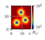
(b) Projected on approx. plane.

Figure 2: Approximation covariance for three measurement points with $\alpha=0.1$, $R_{\text{min}}=10$ and $R_{\text{min}}=100$ for the example measurement points.

Determining the approximation covariance for the whole grid is very time-consuming. Therefore, the calculation is only performed for the grid point at the indices $(i,\,j)\in\mathcal{I}$.

III-C Masked Update

To lower the computational effort and avoid undesired changes outside the approximated region, it is desired to update the mapping only inside the region $\mathcal{A}$. This area is defined by the position of the measurement points on the surface and may have various shapes. In the following, we define index sets $\mathcal{I}$ to construct different binary masks with the elements

$$M_{ij}=\bigg{\{}\begin{array}[]{ll}1&(i,\,j)\in\mathcal{I}\\ 0&\text{else}\end{array}$$ (7)

of an $M\times N$ matrix.

III-C1 Region of interest (ROI) mask

The ROI mask is a rectangular mask, whose size is defined by the minimum and maximum $x$- and $y$-coordinates. Therefore, the elements of the index set $\mathcal{I}$ in (7) fulfill

$$\mathcal{I}:=\{(i,\,j)|\,x_{i}\geq x_{\text{min}}\;\land\;x_{i}\geq x_{\text{max}}\;\land\;y_{j}\leq y_{\text{min}}\;\land\;y_{j}\leq y_{\text{max}}\}$$

with the minimal $x$-coordinate $x_{\text{min}}=\min\{p_{1,\,x},\,\ldots,\,p_{L,\,x}\}$ of the measurement points and maximal $x$- or $y$-coordinate $x_{\text{max}}=\max\{p_{1,\,x},\,\ldots,\,p_{L,\,x}\}$ respectively.

III-C2 Triangular mask

The triangular mask directly gives the convex area between three measurement points. It is defined by considering the triangle edges as

$$\begin{split}&a_{1}=(y_{j}-p_{1,\,y})(p_{2,\,x}-p_{1,\,x})-(p_{2,\,y}-p_{1,\,y})(x_{i}-p_{1,\,x})\\ &a_{2}=(y_{j}-p_{2,\,y})(p_{3,\,x}-p_{2,\,x})-(p_{3,\,y}-p_{2,\,y})(x_{i}-p_{2,\,x})\\ &a_{3}=(y_{j}-p_{3,\,y})(p_{1,\,x}-p_{3,\,x})-(p_{1,\,y}-p_{3,\,y})(x_{i}-p_{3,\,x})\\ &\mathcal{I}:=\{(i,\,j)|\,a_{1}\geq 0\;\land\;a_{2}\geq 0\;\land\;a_{3}\geq 0\},\end{split}$$

where $p_{l,\,x}$ and $p_{l,\,y}$ with $l\in\{1,\,2,\,3\}$ are the $x$- and $y$-coordinates of the measurement points.

III-C3 Largest circle mask

This circular mask includes all measurement points by choosing the mean point ${\boldsymbol{p}}_{c}$ from (2) as the center point of the circle and the radius as the largest distance between this point and all measurement points. Therefore the index set can be written as

$$\mathcal{I}:=\{(i,\,j)|\,(x_{i}-p_{c,\,x})^{2}+(y_{j}-p_{c,\,y})^{2}-r\geq 0\},$$ (8)

where $p_{c,\,x}$ and $p_{c,\,y}$ are the $x$- and $y$-coordinates of the point ${\boldsymbol{p}}_{c}$. The radius is chosen as $r=\max\{r_{l}|\,r_{l}=\sqrt{(p_{l,\,x}-p_{c,\,x})^{2}+(p_{l,\,y}-p_{c,\,y})^{2}},\,\forall l\}$ by projecting the measurement points onto the $xy$-plane of frame $\{0\}$ or $\{A\}$.

III-C4 Circle around points (CAP) mask

Another option is to create a circular mask around each measurement point ${\boldsymbol{p}}_{l}=[p_{l,\,x},\;p_{l,\,y},\;p_{l,\,z}]^{\textrm{\scriptsize{T}}}$ for $l\in\{1,\,\ldots,\,L\}$ with a fixed radius $r$. This is achieved by exploiting (8) to

$$\mathcal{I}:=\bigg{\{}(i,\,j)\bigg{|}\bigvee_{l=1}^{L}(x_{i}-p_{l,\,x})^{2}+(y_{j}-p_{l,\,y})^{2}-r\geq 0\bigg{\}}$$

concatenating single circular masks using the logical or operator. The mask allows additional tuning of the radius.

The described masks are shown in Fig. 3. They are determined in the local frame $\{\text{A}\}$ by transforming the measurement and approximation points using (4) to consider the local geometry, similar to (6). It is also possible to enlarge the boundaries of the mask, e.g., by using the dilation operator, which is known from image processing [20].

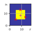
(a) Rectangular ROI mask.

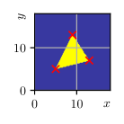
(b) Triangle mask.

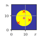
(c) Largest circle mask.

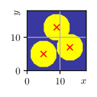
(d) Circle around points mask.

Figure 3: Different mask types projected onto the approximation plane for the example measurement points.

IV EXPERIMENTAL SETUP

The proposed method is tested by mapping an example surface of a computerized numerical control (CNC) manufactured aluminum part with the dimensions $500\times 200\times 50\,$\mathrm{m}\mathrm{m}$$ and a height difference of max. $30\text{\,}\mathrm{mm}$. The surface has a minimal curvature radius of $r_{\text{min}}=1/\kappa_{\text{max}}=$20\text{\,}\mathrm{mm}$$. The surface approximation is performed using three laser distance sensors of type Welotec OWLF 4030 FA S1 with a measurement range between $50$ and $300\text{\,}\mathrm{mm}$. The sensors have a resolution of $0.33\text{\,}\mathrm{mm}$ and a maximum linearization error of $1\text{\,}\mathrm{mm}$ over the full measurement range. They are mounted on a KUKA LBR iiwa 14 robotic manipulator. Together with the forward kinematics of the manipulator, the coordinates of the measured points on the surface are determined. The sensors are tilted by $30\text{\,}\mathrm{\SIUnitSymbolDegree}$ to achieve a smaller approximation area in the vicinity of the tool. The exact tilting angle is identified by a calibration routine using a linear regression of the distance measurements. The analog signals of the distance sensors are evaluated on a Beckhoff CX2000 programmable logic controller (PLC). Figure 4 shows the example surface with the laser distance sensors mounted on the robotic tool.

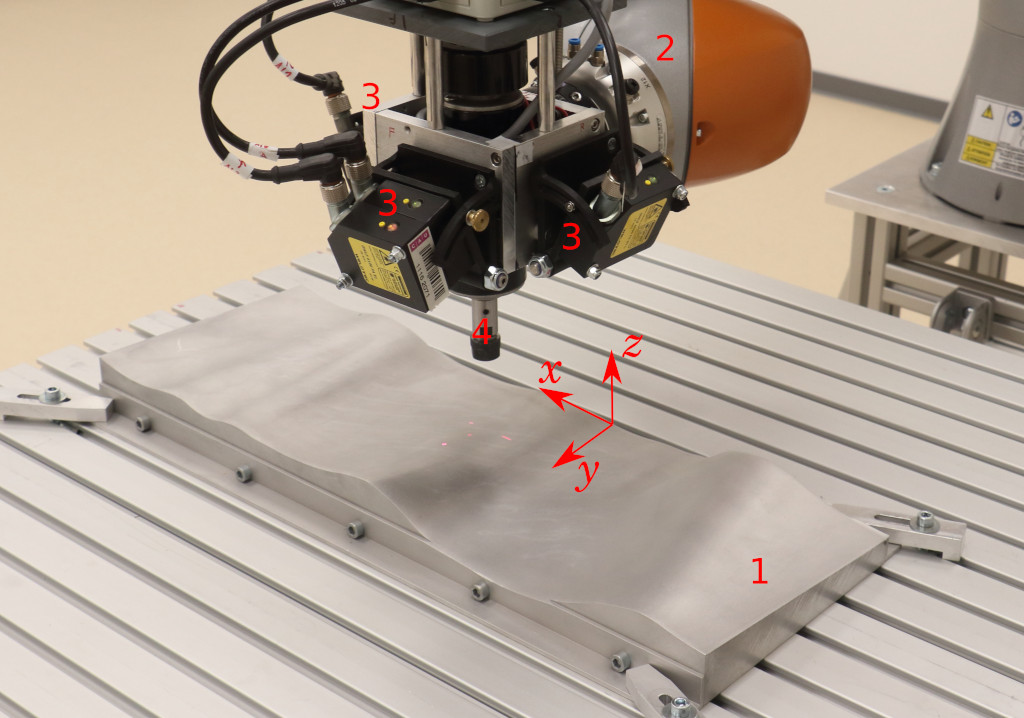
Figure 4: Experimental setup with freeform surface (1) and robotic manipulator (2). The end-effector is equipped with three laser distance sensors (3) and an electric spindle (4).

The surface distance and orientation tracking controller proposed in [15] is used to track the a-priori unknown geometry of the surface. The controller runs on the PLC using the current end-effector pose and the distance measurements to determine the desired pose. This pose is transferred to the KUKA Sunrise robot controller via EtherCAT, where it is continuously commanded to the robotic manipulator using the KUKA Sunrise.Servoing soft real-time interface.

The proposed mapping method is implemented in C and executed as MATLAB MEX file and runs on a separate PC. The algorithm is parallelized using OpenMP, which allows update times of $1.5\text{\,}\mathrm{ms}$ for the used $2\text{\,}\mathrm{mm}$ grid step. It can be either used offline with stored measurements or online where the measured points are received directly from the PLC.

(a) Mapped surface.

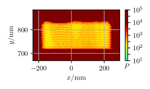
(b) Mapping covariance.

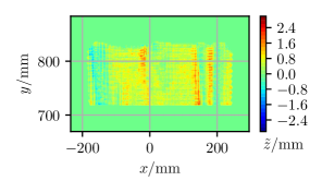
(c) Mapping error.

Figure 5: Mapping results of the constant height trajectory.

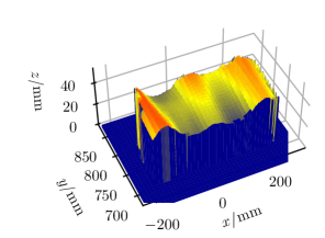
(a) Mapped surface.

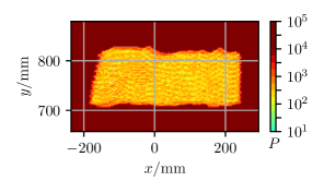
(b) Mapping covariance.

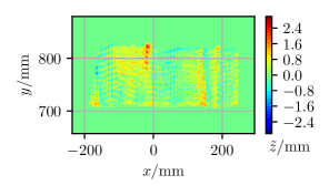
(c) Mapping error.

Figure 6: Mapping results of the surface tracking trajectory.

V RESULTS AND DISCUSSION

The proposed methods are evaluated on the experimental setup described above by mapping the surface of the aluminum part. Here, the robotic manipulator is used to move the distance sensors along the surface. A path is planned with $21$ parallel lines with a distance of $5\text{\,}\mathrm{mm}$ and alternating directions to cover a rectangular area of $400\times$100\text{\,}\mathrm{mm}$$ on the surface. It is executed with a velocity of $25\text{\,}\mathrm{mm}\text{\,}{\mathrm{s}}^{-1}$.

The experiments are performed with the masks defined in Section III-C. For the CAP mask, the radius is set to $5\text{\,}\mathrm{m}\mathrm{m}$. To satisfy a coverage of the surface, even when the approximation area is small, the mask is enlarged using the dilate operation with two grid steps. The parameter $\alpha=0.1$ of the approximation covariance is chosen and the minimum and maximum covariance are set to $R_{\text{min}}=10^{1}$ and $R_{\text{max}}=10^{4}$. This ensures that the approximation covariance functions close to each other overlap.

The mapping update is executed when the distance to the mean point of the last update exceeds $2\text{\,}\mathrm{mm}$. This avoids over-fitting of the approximation plane when the end-effector does not move and ensures that the area covered between two updates is sufficiently large. The measurements between the updates can be used to improve the local approximation.

To evaluate the quality of the mapping, the height $\bar{z}_{ij}$ of the example surface is sampled with one distance sensor at the end-effector, pointing anti-parallel to the $z$-axis of frame $\{0\}$. For the sample points, an equidistant grid of $5\text{\,}\mathrm{mm}$ in the $xy$-plane of the inertial coordinate system is used. The errors are computed by using the mean and maximum absolute value of error $\tilde{z}_{ij}=\hat{z}_{ij}-\bar{z}_{ij}$ between the sample points and the mapping at the $x$- and $y$-coordinates closest to these points. Therefore, only grid points with $\hat{P}_{ij}\leq 10^{4}$ are considered.

TABLE I: Approximation error for different mask types for the constant height and surface tracking trajectory in $\mathrm{mm}$.

Experiment	Mask	Mean Err.	Max. Err.	Std. Dev.
const. height	triangle	0.467	2.073	0.324
	largest circle	0.556	2.978	0.414
	CAP	0.534	1.991	0.295
	ROI	0.694	4.497	0.522
surf. tracking	triangle	0.443	2.554	0.345
	largest circle	0.468	3.650	0.436
	CAP	0.440	3.425	0.402
	ROI	0.572	4.364	0.521

V-A Constant Height Trajectory

In the first experiment, the end-effector tracks the planned path at a constant height over the surface to investigate the influence of approximation area size. Due to the tilt angle of the sensors, the size of the approximation area changes depending on the distance between the surface and the tool.

The mapped surface is shown in Fig. 5(a) based on the triangular mask with dilation. All grid points that are not mapped remain zero. The mapping reconstructs the geometry of the example surface shown in Fig. 4 well. In Tab. I, the mean and maximum absolute mapping errors as well as the error standard deviation, are given for the different mask types described in Section III-C. The CAP mask has the smallest maximum error, while the triangular mask shows the smallest mean error. This may come from the fact that the planar approximation with three measurement points provides a reasonable estimate for the heights in the vicinity of the measurement points as long as the local curvature is small. The triangular mask only contains points, which are between the measurement points and also covers the smallest area of all masks. Therefore, the local approximation does not influence points outside this area.

Figure 5(b) depicts the state covariance of each grid point. There, the contour of the mapped area is clearly visible. Since two laser distance sensor measurements are always performed at the same $y$-coordinate, their paths can be recognized. Because of the constant height of the end-effector and the directions of the distance sensors pointing to a common point, the distance between the measurements decreases for lower areas of the surface. This leads to smaller approximation areas and, therefore, locally smaller approximation covariances. Therefore, also the state covariance is reduced. The area covered by the triangular mask varies between $88$ and $420\text{\,}{\mathrm{mm}}^{2}$, with a mean value of $221\text{\,}{\mathrm{mm}}^{2}$.

Due to the local planar approximation of the surface, the mapping error, shown in Fig. 5(c), is mainly affected by the curvature of the surface. For areas where the curvature is convex, the surface height is underestimated, while in concave areas, it is overestimated. Because of the constant height trajectory, the distance between the measurement points increases for higher surface areas, leading to a larger approximation error in regions with similar curvature. Using a coaxial alignment of the sensors or keeping a constant distance between tool and surface can reduce this effect.

V-B Surface Tracking Trajectory

In the second experiment, the end-effector follows the surface geometry using the distance and orientation controller with a constant distance between end-effector and surface. This leads to the fact that the approximation area remains nearly constant. For example, the triangular mask covers an area between $52$ and $106\text{\,}{\mathrm{mm}}^{2}$, with a mean value of $82\text{\,}{\mathrm{mm}}^{2}$. This is $36\text{\,}\mathrm{\char 37\relax}$ smaller as for the constant height trajectory.

The main deviations between Fig. 5 and Fig. 6 originate from the different scanning paths because of the distance and orientation tracking controller. The mapped heights are shown in Fig. 6(a). While the geometry, in general, is also approximated accurately, it can be noticed that the surface is not as smooth as in the constant height trajectory experiment above. Also, the results in Tab. I show larger maximum errors, while the mean errors are smaller. The reason for this may be that the motion along the unknown surface is not smooth anymore, because the distance and orientation controller must continuously adapt the end-effector pose. Together with some minor but different delays in the measurements of the distance sensors and the end-effector pose, this leads to errors in the estimation of the approximation plane. As shown in Fig. 6(c), the error is independent of the current height of the surface, and the local curvature has a smaller influence due to the small approximation area. The state covariance depicted in Fig. 6(b) also shows that the estimate does not depend on the surface height. Without the dilation of the mask, the surface is not completely mapped, such that some grid points are never updated. This would lead to holes inside the mapping.

During the surface tracking trajectory along the unknown geometry also machining tasks like polishing, grinding or cleaning can be performed. After the surface is covered once, the mapping provides an estimate of the current surface geometry. This can be used to refine the path and trajectory planning for the next execution of the process. In this next execution, the mapping is updated again to improve the estimate of the geometry iteratively. This is especially useful for machining processes, which are repeated multiple times on the same part. The approach is not limited to laser distance sensors such that other types of distance sensors can be used. The mean error, given in Tab. I, is one order of magnitude larger than commercial structured light 3D scanners with an accuracy down to $30\text{\,}\mathrm{\SIUnitSymbolMicro m}$ [21] for a similar measurement volume but is in the range of the accuracy of the robotic manipulator [22]. Therefore, the accuracy of the proposed mapping method is sufficient for the planning of force or impedance-controlled robotic machining tasks or in applications where the manipulator equipped with a compliant end-effector. However, for position controlled tasks with a stiff tool the risk of undesired collisions may occur. The approach can be applied to all industrial robots providing real-time kinematic measurements.

VI CONCLUSION AND FUTURE WORK

The paper proposes a method to map a curved freeform surface using a local planar approximation for scenarios, where only sparse measurements are available, but sensors can be moved along the surface. Linear Kalman filters are used to estimate the height at each grid point. The local measurements are weighted using radial basis functions with a Gaussian kernel to estimate the approximation covariance of the grid points. To update only areas where the approximation is valid different mask types are proposed. The mapping method is evaluated by performing two experiments on an example surface. Here, the robotic manipulator moves the tool equipped with three distance sensors over the surface. Once at a constant height and once by tracking the surface geometry with a distance and orientation controller. Both experiments show that the surface is mapped accurately, while the mapping error depends primarily on the size of the approximation area and the curvature of the surface.

Because the updates of the grid points are independent, the mapping method is well suited for massive parallelization on GPUs. This allows integration into online path planning applications in future works. It is also intended to extend the approach to a SLAM method to improve both the mapping accuracy and the estimate for the tool pose. Another approach is to use higher-order approximations of the local surface geometry, e.g., paraboloid or NURBS, instead of the plane as a first-order approximation. This may require more sensors or can be achieved by exploiting the iterative nature of the method using the previous estimate of the surface geometry.

References

- [1] M. Ren, L. Kong, L. Sun, and C. Cheung, “A Curve Network Sampling Strategy for Measurement of Freeform Surfaces on Coordinate Measuring Machines,” IEEE Transactions on Instrumentation and Measurement, vol. 66, no. 11, pp. 3032–3043, Nov. 2017.
- [2] K. Hansen, J. Pedersen, T. Sølund, H. Aanæs, and D. Kraft, “A Structured Light Scanner for Hyper Flexible Industrial Automation,” in 2014 2nd International Conference on 3D Vision, vol. 1, Dec. 2014, pp. 401–408, iSSN: 1550-6185.
- [3] A. Hennad, P. Cockett, L. McLauchlan, and M. Mehrubeoglu, “Characterization of Irregularly-Shaped Objects Using 3D Structured Light Scanning,” in 2019 International Conference on Computational Science and Computational Intelligence (CSCI), Dec. 2019, pp. 600–605.
- [4] D. Song and Y. J. Kim, “Distortion-free Robotic Surface-drawing using Conformal Mapping,” in 2019 International Conference on Robotics and Automation (ICRA), May 2019, pp. 627–633, iSSN: 2577-087X.
- [5] C.-C. Chu and A. C. Bovik, “Visible surface reconstruction via local minimax approximation,” Pattern Recognition, vol. 21, no. 4, pp. 303–312, Jan. 1988.
- [6] Y. Zhao, J. Zhao, L. Zhang, and L. Qi, “Development of a Robotic 3D Scanning System for Reverse Engineering of Freeform Part,” in 2008 International Conference on Advanced Computer Theory and Engineering, Dec. 2008, pp. 246–250, iSSN: 2154-7505.
- [7] G. Ganesh, N. Jarrassé, S. Haddadin, A. Albu-Schaeffer, and E. Burdet, “A versatile biomimetic controller for contact tooling and haptic exploration,” in 2012 IEEE International Conference on Robotics and Automation, May 2012, pp. 3329–3334, iSSN: 1050-4729.
- [8] D. Song, T. Lee, and Y. J. Kim, “Artistic Pen Drawing on an Arbitrary Surface Using an Impedance-Controlled Robot,” in 2018 IEEE International Conference on Robotics and Automation (ICRA), May 2018, pp. 4085–4090, iSSN: 2577-087X.
- [9] F. Mazzini, D. Kettler, S. Dubowsky, and J. Guerrero, “Tactile robotic mapping of unknown surfaces: an application to oil well exploration,” in 2009 IEEE International Workshop on Robotic and Sensors Environments, Nov. 2009, pp. 80–85.
- [10] F. Mazzini, D. Kettler, J. Guerrero, and S. Dubowsky, “Tactile Robotic Mapping of Unknown Surfaces, With Application to Oil Wells,” IEEE Transactions on Instrumentation and Measurement, vol. 60, no. 2, pp. 420–429, Feb. 2011.
- [11] P. Ozog and R. M. Eustice, “Real-time SLAM with piecewise-planar surface models and sparse 3D point clouds,” in 2013 IEEE/RSJ International Conference on Intelligent Robots and Systems, Nov. 2013, pp. 1042–1049, iSSN: 2153-0866.
- [12] S. Hong and J. Kim, “Three-Dimensional Visual Mapping of Underwater Ship Hull Surface using View-based Piecewise-Planar Measurements,” IFAC-PapersOnLine, vol. 52, no. 21, pp. 384–389, Jan. 2019.
- [13] K. Slatton, M. Crawford, and B. Evans, “Fusing interferometric radar and laser altimeter data to estimate surface topography and vegetation heights,” IEEE Transactions on Geoscience and Remote Sensing, vol. 39, no. 11, pp. 2470–2482, Nov. 2001.
- [14] D. R. Faria, R. Martins, J. Lobo, and J. Dias, “Probabilistic representation of 3D object shape by in-hand exploration,” in 2010 IEEE/RSJ International Conference on Intelligent Robots and Systems, Oct. 2010, pp. 1560–1565, iSSN: 2153-0866.
- [15] M. Amersdorfer, J. Kappey, and T. Meurer, “Real-time freeform surface and path tracking for force controlled robotic tooling applications,” Robotics and Computer-Integrated Manufacturing, vol. 65, p. 101955, Oct. 2020.
- [16] N. J. Mitra and A. Nguyen, “Estimating surface normals in noisy point cloud data,” in Proceedings of the nineteenth annual symposium on Computational geometry, ser. SCG ’03. New York, NY, USA: Association for Computing Machinery, Jun. 2003, pp. 322–328.
- [17] J. Fransens and F. Van Reeth, “Hierarchical PCA Decomposition of Point Clouds,” in Third International Symposium on 3D Data Processing, Visualization, and Transmission (3DPVT’06), Jun. 2006, pp. 591–598.
- [18] M. S. Grewal and A. P. Andrews, Kalman filtering: theory and practice using MATLAB, fourth edition ed. Hoboken, New Jersey: John Wiley & Sons Inc, 2015.
- [19] R. E. Kalman, “A New Approach to Linear Filtering and Prediction Problems,” Journal of Basic Engineering, vol. 82, no. 1, pp. 35–45, Mar. 1960, publisher: American Society of Mechanical Engineers Digital Collection.
- [20] R. C. Gonzalez and R. E. Woods, Digital image processing. New York, NY: Pearson, 2018.
- [21] R. Mendricky and J. Sobotka, “Accuracy Comparison of the Optical 3D Scanner and CT Scanner,” Manufacturing Technology, vol. 20, no. 6, pp. 791–801, Dec. 2020.
- [22] P. Besset, A. Olabi, and O. Gibaru, “Advanced calibration applied to a collaborative robot,” in 2016 IEEE International Power Electronics and Motion Control Conference (PEMC), Sep. 2016, pp. 662–667.