Radiative Supernova Remnants and Supernova Feedback

Abstract

Supernova (SN) explosions are a major feedback mechanism regulating star formation in galaxies through their momentum input. We review the observations of SNRs in radiative stages in the Milky Way to validate the theoretical results on the momentum/energy injection from a single SN explosion. For seven SNRs where we can observe fast-expanding, atomic radiative shells, we show that the shell momentum inferred from Hi 21 cm line observations is in the range of (0.5–4.5)$\times 10^{5}$ $M_{\odot}$ km s^-1. In two SNRs (W44 and IC 443), shocked molecular gas with momentum comparable to that of the atomic SNR shells has been also observed. We compare the momentum and kinetic/thermal energy of these seven SNRs with the results from 1D and 3D numerical simulations. The observation-based momentum and kinetic energy agree well with the expected momentum/energy input from an SN explosion of $\sim 10^{51}$ erg. It is much more difficult to use data/model comparisons of thermal energy to constrain the initial explosion energy, however, due to rapid cooling and complex physics at the hot/cool interface in radiative SNRs. We discuss the observational and theoretical uncertainties of these global parameters and explosion energy estimates for SNRs in complex environments.

1 Introduction

Massive stars have profound impacts on the evolution of the surrounding interstellar medium (ISM), star formation rates, and baryonic cycles in galaxies. The momentum and energy injected by feedback from massive young stars – supernovae (SNe), radiation, and stellar winds – drive turbulence and heat the gas to regulate star formation rates (e.g., McKee & Ostriker, 2007; Krumholz et al., 2014). Stellar population synthesis models imply that the momentum input rates of these feedback processes averaged with stellar initial mass function are more or less similar (e.g., Leitherer et al., 1999; Agertz et al., 2013). However, according to these stellar population synthesis models, the duration of SNe feedback is much longer than those of the other feedback mechanisms (i.e., $\sim 40\,{\rm Myr}$ vs $<5\,{\rm Myr}$ after the birth of stellar population), which makes SNe the most important dynamical feedback mechanism. Furthermore, the energy injection of SNe is highly localized in time and space, creating strong forward and reverse shocks and heating the interior to very high temperature. The subsequent expansion into the ambient medium is nearly adiabatic as long as the shock speed and hence the postshock temperature is high ($T>10^{6}$ K). During the adiabatic stage of evolution, the total injected radial momentum is boosted by more than an order of magnitude (Kim & Ostriker, 2015). Understanding the momentum boosting process and the level of the terminal momentum as a consequence of SNR evolution has practical importance in galaxy formation simulations. In low-resolution simulations, a simple implementation of SN feedback in the form of a thermal energy dump results in immediate loss of energy (a well known overcooling problem; e.g., Katz 1992) due to the inability of resolving the shell formation (or cooling) radius (or mass) (Kim & Ostriker, 2015). Since after reaching a terminal level, the momentum is conserved and not radiated away, injecting the “proper” terminal momentum would be preferred to capture the dynamical impact of SN feedback (e.g., Kimm & Cen, 2014; Hopkins et al., 2014; Rosdahl et al., 2017; Hopkins et al., 2018; Smith et al., 2018, but see Kim & Ostriker 2018; Hu 2019 for a discussion of the other important element of SN feedback, hot gas creation, in galactic scale wind driving).

The momentum boost occurs during the energy conserving stage (also known as the Sedov-Taylor stage; see Sedov 1959; Taylor 1950; Draine 2011). As the SN blast wave sweeps up more and more volume and mass ($R\propto t^{2/5}$ and $M\propto t^{6/5}$) while the energy is conserved, the total radial momentum increases with time $p\propto(ME)^{1/2}\propto t^{3/5}$. When the temperature of shocked gas falls below $\sim 10^{6}$ K as expansion slows down, radiative cooling from metal lines (e.g., highly ionized C, O, and N; see Sutherland & Dopita 1993; Gnat & Ferland 2012) becomes strong and a cold, thin shell forms. Interestingly, since the end of the energy conserving stage (or shell formation) is determined by shock temperature (or expansion velocity), the radial momentum ($p\sim E/v$) at the time of shell formation is nearly independent to the background medium density although the shell formation time itself depends quite sensitively on the mean density of the ISM (e.g., Draine, 2011; Kim & Ostriker, 2015). The evolution of SNRs in a uniform medium is well understood theoretically from both analytic theories (e.g., Cox, 1972; McKee & Ostriker, 1977; Draine, 2011) and direct numerical simulations with radiative cooling (e.g., Chevalier, 1974; Cioffi et al., 1988; Thornton et al., 1998; Blondin et al., 1998).

In recent years, it has become possible to directly simulate SNR evolution in full three dimensions with high resolution. This allows realistic modeling of the background state of the ISM where the SN explodes, including the high degree of inhomogeneity that exists in the real ISM. Several recent numerical simulations have been conducted to include the effect of inhomogeneous background states on SNR evolution. In Kim & Ostriker (2015, KO15 hereafter), a SN explodes in a cloudy two-phase ISM (cold clouds embedded in volume-filling warm diffuse medium) developed from nonlinear saturation of thermal instability. Li et al. (2015) placed a SN in a classical three-phase ISM of McKee & Ostriker (1977), with clouds consisting of cold cores and warm envelopes embedded in a volume-filling hot diffuse medium. Zhang & Chevalier (2019) simulated SNR evolution in a medium realized by driven turbulence. To study SNR expansion within molecular clouds, either an imposed log-normal density distribution (Martizzi et al., 2015; Walch & Naab, 2015) or clouds with driven turbulence (Iffrig & Hennebelle, 2015) has been adopted as a background medium. According to these numerical studies, the momentum of the shell at the time of formation as well as the terminal momentum is insensitive to the background density and hence density inhomogeneity. The resulting final momentum injected to the ISM by a single SN explosion is $p_{\rm SN}=(1-5)\times 10^{5}$ $M_{\odot}$km s^-1 for the canonical explosion energy $E_{\rm SN}=10^{51}{\rm\,erg}$.

Although there is an emerging consensus in theoretical work on the SNR evolution and the final momentum injected to the ISM from a single SN event, observational constraints are still lacking and necessary to validate the theoretical understanding. In addition, there is a missing physical element, cosmic rays, in most studies of SNR evolution, which may or may not have a significant impact (of an order of a few) on the terminal momentum (see Diesing & Caprioli, 2018, but numerical results are sensitive to the model of cosmic ray injection, M. Li et al. in prep). Direct observational constraints on the SNR momentum and energy will play a crucial role to refine theories and identify missing physics in contemporary numerical simulations.

Observationally, it is very difficult to detect radiative shells associated with SNRs. There are about 300 known SNRs in the Milky Way, most of which are identified in radio continuum (Green, 2019). Considering that SNRs spend most of their lifetime in the radiative stage, we expect to see fast expanding shells of atomic hydrogen associated with many of these SNRs. However, because the SNRs are in the Galactic plane, the observation of radiative shells in Hi 21 cm line is severely hampered by the contamination due to the background/foreground Hi emission (e.g., Koo & Kang, 2004). There have been systematic searches for radiative Hi shells associated with the known Galactic SNRs in the northern and southern skies, but the expected fast-expanding Hi shells have been detected only towards a handful of SNRs (Koo & Heiles, 1991; Koo et al., 2004). Another approach to identify radiative Hi shells associated with SNRs is to search for localized high-velocity (HV) Hi features in unbiased Hi surveys of the Galactic plane. The basic idea is that there might be many old, radio-faint SNRs not identified in radio continuum but still possess a fast-expanding Hi shell. The continuing discovery of radio-faint SNRs supports this idea (Foster et al., 2013; Gerbrandt et al., 2014; Driessen et al., 2018; Hurley-Walker et al., 2019). There are a few old radiative SNR candidates identified in this approach (Koo & Kang, 2004; Kang & Koo, 2007; Kang et al., 2014).

In this paper, we inventory the global parameters of radiative SNRs with fast-expanding Hi shells and compare them with the results of 1D and 3D numerical simulations. The global parameters include the momentum and kinetic energy of shocked atomic/molecular gas and also the thermal energy of hot gas. These global parameters are mostly obtained from the literature but, for some SNRs, they are derived in this work. The empirical measurement is not straightforward because we cannot observe all the material engulfed by SN blast wave. This is particularly serious for the Hi shells because we usually observe only the fastest expanding portion of the shell toward or away form us unambiguously. (The Hi emission line in the Galactic plane is very broad due to the Galactic rotation.) Therefore, the estimates of momentum and kinetic energy of expanding Hi shells are obtained from an analysis where it is assumed that the Hi shell is thin and spherical and that the expansion velocity of the shell material is either constant or varying radially. The systematic uncertainties arising from this ‘thin-shell analysis’ might depend on the complexity of the environment, and it is difficult to estimate the uncertainties for individual SNRs. In principle, we can apply the same thin-shell analysis to mock observations from simulations of SNRs, and, by comparing the result with that from observations we can infer the properties of multiphase gas in the environments of individual SNRs and/or we can validate theoretical SNR models. An effort of this kind would, however, require extensive (and numerically costly) parameter space investigation with simulations, given the large possible range of multiphase environments of SNe. As a first step, in this work we take a simpler approach and compare the global parameters derived from the thin-shell analysis to the total momentum and total kinetic/thermal energy of radiative SNRs obtained from numerical simulations. We discuss the uncertainties in the comparison arising from applying the thin-shell analysis for a mock Hi observation of an SNR simulated in the two phase ISM (KO15) as a case study.

The organization of the paper is as follows. In § 2, we first survey the available observations of radiative SNRs and summarize the parameters of their expanding shells. We show that there are seven SNRs (including two old SNR candidates) with Hi shells expanding at $\geq 50$ km s^-1. Four of them are known to be interacting with molecular clouds, and we also summarize the momentum and kinetic energy of shocked molecular gas in these SNRs as well as the thermal energies of the seven SNRs obtained from X-ray observations. In § 3, we compare the observed properties of radiative SNRs with the results from numerical simulations and analyze them. In § 4, we discuss the results and caveats, including the uncertainty in the comparison arising from applying the thin-shell analysis. And in § 5, we conclude our paper.

2 Observed Properties of Radiative SNRs with Hi Shells

In this section, we present basic observed properties of seven radiative SNRs that possess HV Hi shells, mainly from the literature. We then derive momentum and kinetic energy associated with the Hi shells and the molecular gas interacting with the SNRs. We also derive thermal energy of the hot gas from X-ray observations. Although we are not reanalyzing all the observations in this paper (we do for some of them; see Appendix), we summarize the procedures taken to obtain basic quantities to clarify where the uncertainties arise from.

2.1 Hi Shells and Their Momentum and Kinetic Energy

There have been systematic searches for radiative Hi shells associated with the known Galactic SNRs in the northern and southern skies (Koo & Heiles, 1991; Koo et al., 2004). These surveys detected HV Hi gas in 25 SNRs, but because of low angular resolution (i.e., FWHM$=16^{\prime}$–36^′), their association needed confirmation except for the large SNRs, e.g., HB 21 of size $120^{\prime}\times 90^{\prime}$. Among the 25 SNRs, the SNRs confirmed by high-resolution observations are CTB 80 (Koo et al., 1990), W44 (Koo et al., 1995a), W51C (Koo & Moon, 1997), and IC 443 (Giovanelli & Haynes, 1979; Braun & Strom, 1986; Lee et al., 2008). Park et al. (2013) carried out a systematic search for fast-expanding Hi shells toward the SNRs in the Galactic longitude range $\ell\approx$ 32° to 77° using the data from the Inner-Galaxy Arecibo L-band Feed Array (I-GALFA) Hi survey. Their high-resolution study confirmed the Hi shell in G54.4$-$0.3 but did not detect additional SNRs with radiative shells. So there are six SNRs (including HB 21) with their expanding shells studied with high enough spatial resolution. The expansion velocities of expanding Hi shells range 59–135 km s^-1. Among these, the Hi shell in W51C is a partial arc along a large molecular cloud well inside the X-ray/radio SNR that could be the result of multiple SNe (Koo et al. 1995b; Koo & Moon 1997; cf. Tian & Leahy 2013), so the morphology of the SNR-Hi shell system does not fit into a radiative SNR and we exclude the SNR W51C in our analysis.

Another approach is to search for localized HV Hi features in unbiased Hi surveys of the Galactic plane that are not directed specifically at known SNR positions (Koo & Kang, 2004; Kang & Koo, 2007; Kang et al., 2014). Those HV features could be radiative shells associated with old, radio-faint SNRs not identified in radio continuum. Koo & Kang (2004) noted that there are many small, faint, HV “wing-like” features extending to velocities well beyond the maximum or minimum permitted by Galactic rotation in large-scale $(\ell,v)$ diagrams of Hi 21 cm line emission in the Galactic plane and proposed that some of these “forbidden-velocity wings (FVWs)” may represent the expanding shells of “missing” SNRs that are not included in existing SNR catalogs. Koo et al. (2006) have carried out high-resolution Hi line observations toward one of FVWs and showed that it is indeed a rapidly expanding (80 km s^-1) Hi shell and that its physical parameters are consistent with an old SNR (G190.2+1.1). Kang et al. (2012) studied another FVW around Hii  regions at $\ell\sim 173\arcdeg$ and concluded that it is probably an expanding shell associated with an old SNR (G172.8+1.5). These two fast-expanding Hi shell objects are old SNR candidates because their nature as an SNR has not been confirmed. In what follows, however, we will include these two candidates in the analysis.

In summary, there are seven SNRs (including two old SNR candidates) with radiative shells expanding at $\geq 50$ km s^-1 (Table Radiative Supernova Remnants and Supernova Feedback). These middle-aged ($t\sim 10^{4}$–$10^{5}$ yrs) remnants are preferred for measuring the momentum injection quantitatively, since they are old enough to have reached terminal momentum, but not so old that they have started to merge into the background ISM. There have been studies reporting the detection of almost stationary Hi shells or Hi bubbles associated with SNRs (e.g., Kothes et al. 2005; Cazzolato & Pineault 2005; see also references in Koo et al. 2004). But it is difficult to obtain reliable shell parameters for such low-velocity Hi shells, and we limit our study to the seven SNRs in Table Radiative Supernova Remnants and Supernova Feedback. The parameters in Table Radiative Supernova Remnants and Supernova Feedback are from the literature except for HB 21, which are derived in this work (see Appendix A).

In Table Radiative Supernova Remnants and Supernova Feedback, radius ($R_{\rm sh}$), expansion velocity ($v_{\rm sh}$), and Hi mass ($M_{\rm sh}$(Hi)) are obtained directly from radio continuum, Hi 21 cm line, and infrared observations. The method varies for SNRs, which are described briefly in the following. More details may be found in the cited references as well as in Appendix A.

• (1) W44, G54.4$-$0.3, HB21: Middle-aged SNRs with possibly a complete Hi shell. These SNRs appear circular or elliptical loops in radio continuum (e.g., see Figure 1), and the receding portion of an expanding Hi shell is clearly visible inside the remnant including the cap at the center (Koo & Heiles 1991; Park et al. 2013; see also Appendix A). In W44, both the receding and approaching portions are detected. For these SNRs, the radius of the Hi shell is assumed to be the same as the radio continuum loop, while the expansion velocity and the mass of the shell are derived from the average Hi spectrum of the SNR by assuming a spherical thin shell of radius $R_{\rm sh}$ where $R_{\rm sh}$ is the geometrical mean radius for W44 and HB21 which are elliptical.

• (2) IC 443: Middle-aged SNR with a partial Hi shell along the SNR boundary. The SNR appears as two circular loops of different radii in radio continuum, and the portions of an expanding Hi shell are visible along the boundary of the smaller and brighter circular loop in the east (Lee et al. 2008; see also Figure1). In the northern area, both approaching and receding portions of the shell are detected, while in the southern area, where the SNR is interacting with a MC, most of the mass resides in the approaching portion. $M_{\rm sh}$(Hi) is derived from the mass distribution of shocked Hi gas $M(v_{\ell})$ where $v_{\ell}$ is the line of sight (LOS) velocity, either by assuming a Gaussian profile (northern area) or by using the emission profile of shocked molecular gas as a template (southern area) (Lee et al., 2008). The expansion velocity $v_{\rm sh}$ of the shell is assumed to be equal to the shock velocity derived from modeling the optical filaments (Alarie & Drissen, 2019), while the radius of the Hi shell is assumed to be the same as that of the smaller radio continuum loop.

• (3) CTB 80 and G190.2+1.1: Old SNRs with possibly complete shells. The SNR appears either irregular (CTB 80) or is not visible (G190.2+1.1) in radio continuum, but the receding portion of an expanding Hi shell is clearly visible inside the remnant including the cap at the center. In CTB 80, a partially complete, circular infrared loop of shock-heated dust is present, and the radius of the Hi shell is assumed to be the same as this infrared shell (Koo et al., 1990). The expansion velocity of the shell is derived from the Hi line profile at the center (Koo et al., 1990; Park et al., 2013). In G190.2+1.1, which is an old SNR candidate of elliptical shape, the projected size of the shell varies with LOS velocity, which was used to derive the geometrical mean radius and expansion velocity of the shell (Koo et al., 2016). The mass of the shell in these SNRs is derived from the average Hi spectrum of the SNR by modeling $M(v_{\ell})$ with a Gaussian profile assuming spherical symmetry (Park et al., 2013; Koo et al., 2016).

• (4) G172.8+1.5: Old SNR with possibly a complete shell. This is an old SNR candidate that appears as a faint loop of horseshoe-shape in radio continuum (Kang et al., 2012). Diffuse and clumpy Hi emission features with a velocity structure indicating the receding portion of expanding Hi shell are present. The expansion velocity and the mass of the shell are derived from the average Hi spectrum of the SNR by assuming a thick spherical shell of geometrical mean radius $R_{\rm sh}$ with a velocity gradient inside (Kang et al., 2012). The radius of the Hi shell is assumed to be the same as the radio continuum loop.

The momentum ($p_{\rm sh}$) and the kinetic energy ($E_{\rm K,sh}$) of the shell are derived from $M_{\rm sh}$(Hi) and $v_{\rm sh}$; $p_{\rm sh}=M_{\rm sh}v_{\rm sh}$ and $E_{\rm K,sh}=M_{\rm sh}v_{\rm sh}^{2}/2$ where $M_{\rm sh}(=1.4M_{\rm sh}$(Hi)) is the mass of shell including the contribution from He assuming cosmic abundance. The parameter $t_{\rm sh}$ is the characteristic age of the shell defined as

$$t_{\rm sh}\equiv 0.3{R_{\rm sh}\over v_{\rm sh}}.$$ (1)

This characteristic age $t_{\rm sh}$ should be close to the age of the SNR if the SNR is in the pressure-driven snowplow (PDS) phase. But the expansion parameter $\eta$ ($R\propto t^{\eta}$) that appears as a prefactor in Equation (1) could vary from 0.4 to 0.25 depending on the evolutionary state of the SNR so that it could be slightly different from the true age. According to Table Radiative Supernova Remnants and Supernova Feedback, the radiative Hi shells of our sample of SNRs have $p_{\rm sh}=(0.5$–$4.5)\times 10^{5}$ $M_{\odot}$ km s^-1, $E_{\rm K,sh}=(0.4$–$3.5)\times 10^{50}$ erg, and $t_{\rm sh}=(0.3$–$3.4)\times 10^{5}$ yr.

There are some caveats in using the physical parameters in Table Radiative Supernova Remnants and Supernova Feedback. First, the observed Hi mass is only a small fraction of the total shell mass because only the portions of the shell with high enough LOS velocities are visible. So the parameters $M_{\rm sh},p_{\rm sh},E_{\rm K,sh}$ are obtained by applying the thin-shell analysis where it is assumed that the Hi shell is thin and spherical and that the expansion velocity of the shell material is either constant or varying radially depending on the observed properties of the Hi 21 cm emission. The systematic uncertainties arising from this thin-shell analysis might depend on the complexity of the environment, and it is difficult to quantify the errors for individual SNRs. (Note that the errors in Table Radiative Supernova Remnants and Supernova Feedback are formal errors associated with the measurement errors.) The parameters $M_{\rm sh},p_{\rm sh},E_{\rm K,sh}$ in Table Radiative Supernova Remnants and Supernova Feedback should be understood as those derived from the thin-shell analysis. We will discuss the systematic uncertainties in the thin-shell analysis in § 4.2. Second, the distance ($d$) to the SNRs is uncertain. The uncertainty in the distances in Table 1 is probably $\lower 2.15277pt\hbox{$\;\buildrel<\over{\sim}\;$}30$ % except for G 190.2$+$1.1. For G190.2$-$1.1, there is only circumstantial evidence and 8 kpc has been suggested to yield the SN explosion energy of $10^{51}$ erg (Koo et al., 2006). Note that $M_{\rm sh}\propto d^{2}$, so that the uncertainty of 30 % in $d$ yields $p_{\rm sh}$ and $E_{\rm K,sh}$ uncertain of 60%.

2.2 Shocked Molecular Gas and Its Momentum and Kinetic Energy

Among the seven SNRs in Table Radiative Supernova Remnants and Supernova Feedback, four SNRs are known to be interacting with MCs: W44, G54.4$-$0.3, HB 21, and IC 443 (see Note in Table Radiative Supernova Remnants and Supernova Feedback). W44 and IC 443 are the two prototypical SNRs interacting with large MCs (Figure 1). The presence of both shocked atomic (Hi) and shocked molecular (e.g., CO and HCO⁺) gases in these SNRs can be explained by SN explosion inside a clumpy or turbulent MC. In such case, the shocked molecular gas usually represents non-dissociative shock propagating into the dense clumps while the HV Hi gas is from a radiative atomic shock propagating into the rather diffuse interclump gas (Chevalier & Li, 1999; Reach et al., 2005; Koo et al., 2014; Zhang & Chevalier, 2019). This model can also explain the centrally-brightened X-ray emission (see § 2.3). In addition to the clumpiness, the molecular line emission confined to one side of the SNR suggests a surrounding medium with a large-scale density gradient where thermal conduction can substantially alter the interior structure of an SNR (Cox et al., 1999). In § 4, we will discuss the effect of such complex environment in analyzing the observed global parameters. In the other SNRs, the shocked molecular gas is either not prominent or has not been detected (see Note in Table Radiative Supernova Remnants and Supernova Feedback).

The momentum and kinetic energy of shocked molecular gas can be derived from the molecular line emission from shocked molecular gas. Table Radiative Supernova Remnants and Supernova Feedback summarizes the results available in the literature. In Table Radiative Supernova Remnants and Supernova Feedback, the mass of H₂ ‘shell’ ($M_{\rm sh}$(H₂)) represents the mass of shocked molecular H₂ gas obtained from the emission line flux of molecules such as HCO⁺ and CO, and there is a large ($\sim 50$ %) uncertainty in scaling the emission line flux to H₂ mass. The expansion velocity ($v_{\rm sh}$) is derived from a fit to the velocity structure (W44, IC 443) or from the mean velocity of shocked molecular clumps (HB 21). The momentum ($p_{\rm sh}$) and the kinetic energy ($E_{\rm K,sh}$) of the shocked molecular gas are derived from $M_{\rm sh}$(H₂) and $v_{\rm sh}$ as in Hi shell, i.e., $p_{\rm sh}=M_{\rm sh}v_{\rm sh}$ and $E_{\rm K,sh}=M_{\rm sh}v_{\rm sh}^{2}/2$ where $M_{\rm sh}=1.4M_{\rm sh}$(H₂). According to Table Radiative Supernova Remnants and Supernova Feedback, in W44 and IC 443, the momentum of shocked molecular gas is comparable to or even larger than that of the Hi shell (1.8 and $0.7\times 10^{5}$ $M_{\odot}$ km s^-1), while its kinetic energy is relatively small ($\lower 2.15277pt\hbox{$\;\buildrel<\over{\sim}\;$}0.2\times 10^{50}$ erg). For G54.4$-$0.3, large MCs are around the SNR and it has been proposed that this ‘molecular shell’ is expanding at 5 km s^-1, in which case its momentum would be $\sim 1\times 10^{6}$ $M_{\odot}$ km s^-1 (Junkes et al., 1992a). But there is no convincing evidence that the large MCs are shocked and/or expanding. Instead, there are small, thin H₂ 2.122 $\mu$m emission filaments implying a small amount of shocked molecular gas (see Note in Table Radiative Supernova Remnants and Supernova Feedback). For HB 21, the momentum and kinetic energy of shocked molecular gas are not significant. For the remaining three SNRs, the shocked molecular gas has not been detected, so that the momentum and kinetic energy of shocked molecular gas might not be significant.

2.3 Hot Gas and Its Thermal Energy

Six SNRs are detected in X-ray, and the physical parameters of the X-ray emitting hot gas including its thermal energy are listed in Table Radiative Supernova Remnants and Supernova Feedback. All results are obtained from the literature except G54.4$-$0.3 and CTB 80, for which we derive it in this paper (see Appendices B.1 and C). Table Radiative Supernova Remnants and Supernova Feedback shows that the mean density of the hot gas in six SNRs is in the range of 0.006–2 cm^-3, while the temperature of hot gas is $<1$ keV. The thermal energy of the hot gas is in the range of 0.6–$8\times 10^{50}$ erg.

The parameters in Table Radiative Supernova Remnants and Supernova Feedback are derived from spectral analysis except G172.8$+1.5$ where the X-ray emission is seen only in the broad band ROSAT all-sky X-ray map. The X-ray spectral analysis provides the electron temperature ($T$) and the normalization factor proportional to $EM/4\pi d^{2}$ where $EM=\int n_{e}n_{\rm H}dV$ ($n_{e}$, $n_{\rm H}$ = electron and hydrogen densities) is the volume emission measure and $d$ is the distance to the source. Therefore, the average electron density in terms of $EM$ is given by $\bar{n}_{e}=g_{e}^{1/2}(EM/V_{EM})^{1/2}\propto d^{-1/2}$ where $g_{e}=n_{e}/n_{\rm H}\approx 1.2$ and $V_{EM}$ is the volume of the X-ray emitting hot plasma. The uncertainty of 30 % in $d$ yields $E_{\rm th}$ uncertain by a factor of $\sim 2$. It is worthwhile to note that $V_{EM}$ is often considerably smaller than the SNR because the area used for the X-ray spectral analysis is limited. For G54.4$-$0.3 and CTB 80, for example, the area is limited to the X-ray bright part of the SNRs and we, for a simple approximation, assumed that the hot plasma is uniformly filling a cylindrical volume with a path length (along the line of sight) corresponding to the physical diameter of the spherical SNR (Appendices B.1 and C). For the other sources, see Note in Table Radiative Supernova Remnants and Supernova Feedback. A major uncertainty in the total thermal energy of an SNR arises from the geometry of hot gas. The SNRs in general have non-uniform X-ray brightness, which might be due to the combination of temperature/density/metallicity structure and varying absorbing columns. In W44, for example, it has been shown that the X-ray emission filling the interior is faint near the SNR shell because of low electron temperature and large absorbing columns (see Fig. 1; Okon et al. 2020). For this study, we derive the thermal energy of SNRs assuming that the entire interior volume of the SNRs is filled with hot gas in pressure equilibrium, i.e., $E_{\rm th}\approx 3{\bar{n}_{e}}k_{B}TV_{s}$ where $k_{B}$ is the Boltzmann constant and $V_{s}(\equiv 4\pi R_{s}^{3}/3)$ is the total volume of the SNR. (For IC 443, we assumed two hemispherical spheres following Troja et al. 2006. Some notes on individual SNRs are given in Table Radiative Supernova Remnants and Supernova Feedback.) We note that our assumption of a spherical volume of radius $R_{s}$ might be an over-simplification to yield an overestimate of the volume in general, although the pressure equilibrium might be a reasonable assumption. The systematic uncertainties in the thermal energy estimate due to the uncertainties in the geometry of an SNR, e.g., the extent along the LOS and the volume filling factor of hot gas, are difficult to estimate. The thermal energies in Table Radiative Supernova Remnants and Supernova Feedback should be understood as those obtained by assuming a spherical volume filled with hot gas in pressure equilibrium. If the volume filling factor of hot gas is $\sim 0.5$, then the thermal energy would be $\sim 1/2$ of that in the table (see § 4.1 and § 4.2).

It is worth making a comment on the X-ray morphology of SNRs. As we can see in Figure 1, the X-ray brightness in some SNRs is centrally peaked, not limb brightened as we expect in an ‘ideal’ SNR. Essentially all six SNRs visible in X-ray have such X-ray morphology including CTB 80 with peculiar radio morphology and the old SNR G172.8+1.5. They belong to the so-called “thermal composite” or “mixed-morphology” SNRs (hereafter MM SNRs) which are the SNRs that are shell or composite type in radio but with centrally-brightened thermal X-rays inside the SNR (Rho & Petre, 1998; Lazendic & Slane, 2006; Vink, 2012). Most of these MM SNRs are thought to be middle-aged SNRs interacting with dense ISM, e.g., molecular clouds (Zhang et al., 2015; Slane et al., 2015; Koo et al., 2016). W44 and IC 443 are prototypical MM SNRs. The origin of the centrally-brightened thermal X-ray is not clear (Slane et al., 2002; Lazendic & Slane, 2006; Vink, 2012; Slane et al., 2015). The proposed scenarios are (1) absorption of soft X-rays from near the edge of the remnant by the large absorbing column density (Harrus et al., 1997; Velázquez et al., 2004), (2) large-scale conduction between the hot interior and the cool SNR shell (Cox et al., 1999; Shelton et al., 1999; Velázquez et al., 2004; Tilley et al., 2006; Okon et al., 2020), and (3) evaporation of small, dense clumps engulfed by SN blast wave (White & Frenk, 1991; Slavin et al., 2017; Zhang et al., 2019). In some SNRs, it has been found that heavy elements are enriched, which can partly responsible for the centrally-brightened X-ray emission (see Lazendic & Slane 2006; Vink 2012 and references therein). In several MM SNRs, it has been also found that the hot plasma is overionized implying a rapid cooling, but its relation to the X-ray morphology is not clear (e.g., Slane et al. 2015 and references therein). Recently, there have been 2D and 3D numerical simulations in clumpy or turbulent media to understand the origin of MM SNRs (Slavin et al., 2017; Zhang & Chevalier, 2019; Zhang et al., 2019), but the role of thermal conduction in thermal energy evolution remains to be explored (see section 4.3).

3 Integrated Properties of Radiative SNRs

3.1 Observed Global Parameters

Table 4 summarizes the observed global parameters of radiative SNRs; $p_{\rm sh}$, $E_{\rm K,sh}$, and $E_{\rm th}$. For SNRs with shocked molecular gas, $p_{\rm sh}$ and $E_{\rm K,sh}$ of the atomic (Hi), molecular (H₂), and atomic+molecular components are given. The table shows that the total (Hi+H₂) momentum and kinetic energy of the radiative SNRs are in the range of $p_{\rm sh}=$(1.1–4.5)$\times 10^{5}$ $M_{\odot}$km s^-1 and $E_{\rm K,sh}=$(0.6–3.5)$\times 10^{50}$ erg, respectively, while $E_{\rm th}=(0.6-8)\times 10^{50}$ erg. In the table, $\bar{n}_{\rm bg}$ is the density of hydrogen nuclei if the mass of shocked atomic/molecular gas were uniformly filling the spherical volume of radius $R_{\rm sh}$.

If the ambient medium is isotropic, $\bar{n}_{\rm bg}$ in the ‘Hi+${\rm H}_{2}$’ column of Table 4 will be close to the mean density of the ambient medium, in which SN blast waves propagate, even if the medium is inhomogeneous. It is, however, not unusual that the ambient medium has a large-scale non-uniformity for SNRs, e.g., SNRs produced inside or outside large MCs near their surface (Tenorio-Tagle et al., 1985; Jeong et al., 2013; Cho et al., 2015; Iffrig & Hennebelle, 2015, and references therein). For example, IC 443 in Figure 1 is interacting with a dense MC in the southern area and the shocked atomic and molecular gases are mainly confined to that area. The density in the northern area where the X-ray emission is prominent could be significantly lower than the total mean density. W44, on the other hand, appears to be located inside an MC (Chevalier & Li, 1999; Zhang & Chevalier, 2019). But again, most of the cool, shocked molecular gas is confined to the eastern area (e.g., Sashida et al., 2013, see also Figure 1). The mean ambient density inferred from Hi and X-ray observations ($\lower 2.15277pt\hbox{$\;\buildrel<\over{\sim}\;$}10$ cm^-3, see Koo et al. 1995b; Chevalier & Li 1999; Zhang & Chevalier 2019 and references therein) is indeed much lower than the average density when the shocked atomic and molecular gases were uniformly filling the spherical volume of the SNR (i.e., 50–70 cm^-3, Table 4). One therefore needs to be cautious in using the characteristic densities in Table 4, particularly for SNRs interacting with MCs (see Note in Table Radiative Supernova Remnants and Supernova Feedback for a brief description of individual SNRs).

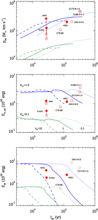
Figure 2: Observation-based momentum ($p_{\rm sh}$), kinetic energy ($E_{\rm K,sh}$), and thermal energy ($E_{\rm th}$) of the SNRs with fast-expanding Hi shells. The $x$-axis is the characteristics age of the Hi shell $t_{\rm sh}=0.3R_{\rm sh}/v_{\rm sh}$. The open circles represent the Hi component only, while the filled circles include the contribution from shocked molecular gas. For the SNRs marked only with open circles, the contribution from molecular component is not significant (see Table Radiative Supernova Remnants and Supernova Feedback). Note that $p_{\rm sh},E_{\rm K,sh}$ and $E_{\rm th}$ are obtained by assuming that the Hi shell is thin and spherical and that the hot gas is filling the interior of the SNR (see text for more details). The formal errors are small and not shown here (see Tables Radiative Supernova Remnants and Supernova Feedback–Radiative Supernova Remnants and Supernova Feedback). Also shown are theoretical evolutionary tracks obtained from 1-D hydrodynamic simulations of expansion into a uniform medium. The blue and green lines are for SN explosion energies $E_{\rm SN}=10^{51}$ and $10^{50}$ erg, respectively, while the dotted, solid, and dashed lines represent different ambient densities ($n_{0}=(n_{\rm bg}/1~{}{\rm cm}^{-3})=0.1,1$, and 10).

Bearing the above caveats in mind, we show in Figure 2 the observed momentum and energy of the SNR as a function of $t_{\rm sh}$. For comparison, we also plot theoretical evolutionary tracks obtained from 1-dimensional hydrodynamic simulations using Athena++ (Stone et al., 2020), in which we follow the evolution of SNRs in a uniform medium with spherical symmetry including radiative cooling and thermal conduction (see El-Badry et al., 2019, for details). For theoretical curves, we use the true age of the SNR $t_{\rm sh}=t$ not $t_{\rm sh}=0.3R_{\rm sh}/v_{\rm sh}$ as the $x$-axis, e.g., we plot $p_{\rm sh}(t_{\rm sh}=t)$ not $p_{\rm sh}(0.3R_{\rm sh}/v_{\rm sh})$. The difference in momentum by using $t$ not $t_{\rm sh}$ is $\lower 2.15277pt\hbox{$\;\buildrel<\over{\sim}\;$}10$% before the shell formation time and is negligible after that. For kinetic energy, the difference is almost negligible before the shell formation time and slowly increases to 5 % until the final stage. Considering the uncertainty in observed parameters and the idealization of the spherically symmetric simulations, we simply use $t$ for the theoretical curves.

In Figure 2, it is remarkable to see that the observed momenta of seven SNRs are all very close to the theoretical result for the canonical SN explosion energy $E_{51}\equiv(E_{\rm SN}/10^{51}~{}{\rm erg})=1.0$. W44, for example, has a momentum corresponding to an SNR in the momentum-conserving phase in dense environment of mean ambient density $n_{0}\equiv(n_{\rm bg}/1~{}{\rm cm}^{-3})\lower 2.15277pt\hbox{$\;\buildrel>\over{\sim}\;$}10$ where $n_{\rm bg}$ is the hydrogen number density of the uniform background medium. As we pointed out above, the ambient density may vary considerably for a given SNR as well as from SNR to SNR. But, since the SNR momentum is insensitive to ambient density but sensitive to SN explosion energy, i.e., $p_{\rm sh}\propto n_{0}^{-1/7}E_{51}^{13/14}$ (e.g., Cioffi et al., 1988; Thornton et al., 1998; Kim & Ostriker, 2015), the SN explosion energy smaller or greater than the canonical value by a factor of 2–3 can explain the observed range of the SNR momentum. The observed range of the SNR kinetic energy (0.6–3.5$\times 10^{50}$ erg) also matches the theoretical result for $E_{51}\sim 1$. IC 443 appears to be far from the theoretical curve with $E_{51}=1.0$ but, since its mean ambient density is $\sim 60$ cm^-3, $E_{51}\sim 0.5$ can explain the kinetic energy.

The thermal energy has a relatively large scatter; CTB 80 has thermal energy of 6$\times 10^{49}$ erg while the other SNRs have thermal energies much larger than this (2–8$\times 10^{50}$ erg). The large scatter might be partly because the thermal energy sensitively depends on both $n_{0}$ and $E_{\rm SN}$, i.e., $E_{\rm th}\propto E_{51}^{1.35}n_{0}^{-0.86}$ (§ 3.2). Therefore, again the SN explosion energy smaller or greater than the canonical value by a factor of 2–3 can explain the observed range of the SNR thermal energy, although the corresponding density does not yield the observed momentum and kinetic energy. One thing to notice is that the observed thermal energies are generally greater than the theoretical result for $E_{51}=1$ in contrast to the observed shell momenta and kinetic energies which are generally smaller than the theoretical result for $E_{51}=1$. HB 21, for example, has thermal energy that is not particularly large (i.e., $E_{\rm th}\sim 2\times 10^{50}$ erg) but, since the SNR thermal energy decreases slightly super-linearly with time after the shell formation, it is still significantly greater than the expected thermal energy for $E_{51}=1$ and $n_{0}=1$. The same is true for W44 and IC 443; their thermal (kinetic) energies are larger (smaller) than those expected for $E_{51}=1$ and $n_{0}=10$. The only SNR that has thermal energy smaller than the theoretical result for $E_{51}=1$ is CTB 80. We consider that this discrepancy is due to the complex environments of the SNRs, and we will discuss this in § 4.1 and § 4.2.

3.2 Comparison with Simulations

The real ISM is highly inhomogeneous and structured. Therefore, the comparison with the model SNR evolution within a uniform medium is possibly too simplistic. In this subsection, we present evolutionary tracks of the integrated SNR properties from a variety of numerical simulations to understand systematic uncertainties in theoretical models.

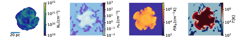
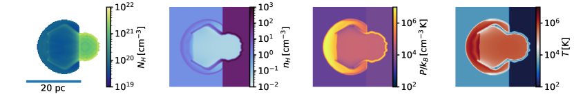
Figure 3: From left to right, we show SNR column density and slices of number density, thermal pressure, and temperature. The SNR component is selected by $T>2\times 10^{4}{\rm\,K}$ and $|v|>1{\rm\,km\,s^{-1}}$ (see KO15). 20 pc scale bars are shown on the bottom left corner of the column density panels. Top Row: An example snapshot at $t=0.03{\rm\,Myr}$ of a TI model with mean hydrogen number density $\bar{n}_{\rm bg}=1$ cm^-3. The two phase medium is produced by running a thermal instability simulation for 200 Myr to reach a nonlinear saturation state. The CNM and WNM have typical hydrogen number density of $\sim 9{\rm\,cm^{-3}}$ and $\sim 0.15{\rm\,cm^{-3}}$, respectively. Bottom Row: An example snapshot of a TS model with the explosion depth $h=2{\rm\,pc}$ at $t=0.03{\rm\,Myr}$. The density of two medium is 1 and $100{\rm\,cm^{-3}}$. For references, the shell formation times in uniform media with $n_{\rm bg}=0.1$, 1, 10, and 100 cm^-3 are $t_{\rm sf}=0.16$, 0.044, 0.012, and 0.0035 Myr. Therefore, blast waves already cool in the CNM of the TI model and the dense medium of the TS model.

To explore the role of ambient conditions, we use additional 3D hydrodynamic simulations including two kinds of initial background medium states: (1) inhomogeneous background medium as a result of thermal instability (TI model; see KO15) and (2) contacting two homogeneous slabs (TS model; see Cho et al. 2015). Figure 3 shows example snapshots from TI (top) and TS (bottom) models. For the TI model, we first run a simulation with initially thermally unstable equilibrium state and let it evolve toward a nonlinear saturated state of thermal instability (Field, 1965; Piontek & Ostriker, 2004; Kim et al., 2008; Choi & Stone, 2012; Inoue & Omukai, 2015). The resulting medium consists of two distinct thermal phases in the pressure equilibrium, namely cold neutral medium and warm neutral medium (CNM and WNM, respectively), with density and temperature contrasts about 100. The WNM is volume filling ($\sim 90$%), while the CNM comprises most of the mass ($\sim 80$%). As a result, the TI model provides a natural way to set up a clumpy ISM, with characteristics determined by cooling and heating processes of the ISM (e.g., Field, 1965; Field et al., 1969; Wolfire et al., 1995; Bialy & Sternberg, 2019). We use 10 realizations of the TI model with mean hydrogen density of $\bar{n}_{\rm bg}=1$ cm^-3 and $\bar{n}_{\rm bg}=10$ cm^-3, while we show an example for the $\bar{n}_{\rm bg}=1$ cm^-3 case in the top row of Figure 3. We refer the readers KO15 for complete descriptions of model setups and more comprehensive parameter study. The TS model is characterized by the densities of two media (which are fixed to $n_{\rm bg}=1{\rm\,cm^{-3}}$ and $100{\rm\,cm^{-3}}$ here) and the explosion depth from the contacting surface toward the denser medium $h$. We present seven different explosion depths varying from $h=-1$, 0, 1, 2, 2.5, 3, and 4 pc, while we show an example for the $h=2{\rm\,pc}$ case in the bottom row of Figure 3. We refer the readers Cho et al. (2015) for complete descriptions of model setups and more comprehensive parameter study.

Note that the background medium realizations presented here are by no means a complete census of SN explosion sites. We show two representative examples to demonstrate possible variations of SNR evolution due to background medium states, but there are many other possible realizations (e.g., Li et al., 2015; Martizzi et al., 2015; Walch & Naab, 2015; Iffrig & Hennebelle, 2015; Zhang & Chevalier, 2019).

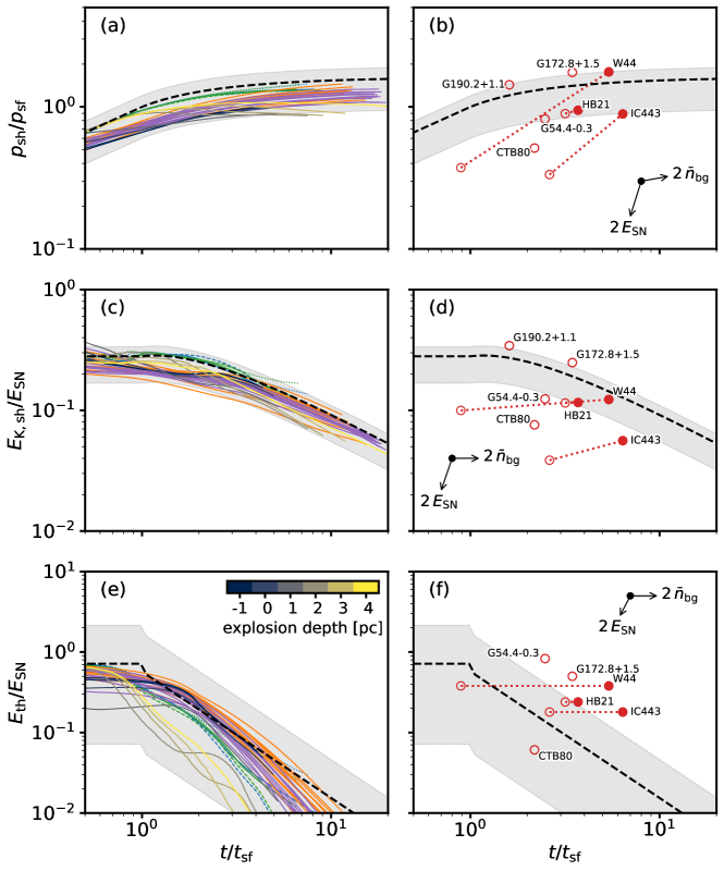
Figure 4: Left Column: Evolution of (a) total radial momentum, (c) kinetic energy, and (e) thermal energy of the simulated SNRs. The properties of SNRs are normalized by the quantities at the shell formation (i.e., $t_{\rm sf}$ and $p_{\rm sf}$; see § 3) and the explosion energy. The simulated evolution tracks of SNRs in a uniform medium (blue and green lines same as Figure 2) are almost congruent for the normalized properties. The analytic model (Eqs. 11 and 12) describing the 1D model is shown as black dashed line. The evolution tracks from the TI models are shown as two groups of solid lines ($\bar{n}_{\rm bg}=1$ cm^-3 for orange and $\bar{n}_{\rm bg}=10$ cm^-3 for purple), each of which corresponds 10 realizations of the background medium as a result of thermal instability. The evolution tracks from the TS models are color coded by the explosion depth from the interface toward the denser medium as indicated by the legend in (e). Both evolution tracks generally follow the analytic model, especially for momentum and kinetic energy. The gray shaded region covers the arbitrarily rescaled analytic models to gauge model uncertainties in describing simulations. The area spans 0.6-1.2$\times$ the model for momentum and kinetic energy and 0.1-3$\times$ the model for thermal energy. Right Column: Observed SNR properties normalized by the quantities at the shell formation using the ambient medium density ($\bar{n}_{\rm bg}$ in Table 4; either Hi only or Hi+H₂) and the canonical explosion energy ($E_{\rm SN}=10^{51}$ erg). The vectors in each panel show the directions for systematic uncertainties of $E_{\rm SN}$ and $\bar{n}_{\rm bg}$ adopted for each SNR. The same analytic model curve and area is duplicated for comparison.

Figure 4 presents evolutionary tracks of the integrated SNR properties from all numerical simulations (left column for (a) total radial momentum, (c) kinetic energy, and (e) thermal energy), including the 1D spherically symmetric simulations in a homogeneous medium presented in Figure 2. In Figure 4, the physical quantities are normalized by the parameters at the shell formation, i.e.,

$$t_{\rm sf} = 4.4\times 10^{4}{\,\rm yr}\,E_{51}^{0.22}n_{0}^{-0.55},$$ (2)

$$p_{\rm sf} = 2.17\times 10^{5}{\,M_{\odot}\,{\rm km~{}s}^{-1}}\,E_{51}^{0.93}n_{0}^{-0.13}$$ (3)

(Eqs. 7 and 17 in KO15) and the explosion energy used in the simulations. Note that $n_{0}=n_{\rm bg}/1~{}{\rm cm}^{-3}$ and that we again use the true age ($t$) of SNR for the $x$-axis. For $n_{0}$, we use the mean density of the whole SNR bubble defined by gas with $T>2\times 10^{4}$ K or $|v|>1$ km s^-1 (e.g., KO15). For the TI models, $n_{0}$ is nearly constant over time, while it varies with time for the TS models. For reference, $t_{\rm sf}=156$, 44, 12, and 3.5 kyr for $n_{0}=0.1$, 1, 10, and 100, respectively. Noticeably, simulations with different background realizations follow very similar evolutionary tracks for momentum and kinetic energy, while the thermal energy evolution can vary significantly.

The model prediction of total radial momentum and kinetic energy (after the shell formation) for a given explosion energy is quite robust irrespective of the complexity of the explosion environment. This is mainly due to (1) weak dependence and no dependence on the mean density respectively of momentum and kinetic energy at shell formation and (2) a minimal increase/decrease of momentum and kinetic energy after the shell formation. Despite a wide variety of background conditions considered here, total momentum/kinetic energy in simulations after shell formation differs by less than a factor of 2. As a consequence, total momentum and kinetic energy measured theoretically for radiative SNRs are not sensitive to the mean density but to the explosion energy.

This motivates us to map the global properties of observed SNRs into the normalized quantity plane in the right column of Figure 4. To calculate the normalization factors $t_{\rm sf}$ and $p_{\rm sf}$ from Equations (2) and (3) for observed SNRs, we adopt $\bar{n}_{\rm bg}$ in Table 4 and the canonical explosion energy $E_{\rm SN}=10^{51}$ erg. For SNRs with associated MCs, two observation points are shown not only for total radial momentum and kinetic energy excluding and including H₂ contributions but also for different $t_{\rm sf}$ and $p_{\rm sf}$ derived from $\bar{n}_{\rm bg}($Hi$)$ and $\bar{n}_{\rm bg}($Hi$+{\rm H}_{2})$ as open and filled circles, respectively, connected by a dotted line. As we adopt a fixed value for $E_{\rm SN}$ and the uncertainty in $\bar{n}_{\rm bg}$ is dominated by systematic errors, the uncertainties of observed SNRs in Figure 4 are not well defined and difficult to present. We instead show two vectors in panels (b), (d), and (e) to present how the observation points would move if $\bar{n}_{\rm bg}$ or $E_{\rm SN}$ is increased by factor of two. For momentum, the $\bar{n}_{\rm bg}$ vector is almost parallel to the theoretical curve (dashed line; see below) after shell formation time. For kinetic energy, the $\bar{n}_{\rm bg}$ vector is horizontal, while the theoretical evolution track falls sub-linearly with time. This allows us to derive the explosion energy of SNRs using momentum and kinetic energy reliably assuming the momentum and kinetic energy inferred from the described observations comprise the majority of these quantities.

To get the explosion energy, we use analytic expressions for radius and momentum evolution during the Sedov-Taylor and post shell formation stages (e.g., KO15):

$$R_{\rm sh} = \left\{\begin{array}[]{lc}r_{\rm sf}(t/t_{\rm sf})^{2/5}&\quad\textrm{if $t<t_{\rm sf}$}\\ r_{\rm sf}(t/t_{\rm sf})^{2/7}&\quad\textrm{otherwise,}\end{array}\right.$$ (6)

$$p_{\rm sh} = \left\{\begin{array}[]{lc}p_{\rm sf}(t/t_{\rm sf})^{3/5}&\quad\textrm{if $t<t_{\rm sf}$}\\ p_{\rm sf}(1+0.62(1-(t/t_{\rm sf})^{-6/7}))&\quad\textrm{otherwise,}\end{array}\right.$$ (9)

where

$$r_{\rm sf}=22.6E_{51}^{0.29}n_{0}^{-0.42}\quad{\rm pc}$$ (10)

is the radius at the time of shell formation. Then, the kinetic energy can be calculated $E_{\rm K,sh}=p_{\rm sh}^{2}/(2M_{\rm sh})$, where $M_{\rm sh}=(4\pi/3)R_{\rm sh}^{3}\rho_{\rm bg}$. As $t\gg t_{\rm sf}$, the terminal momentum approaches to $1.6p_{\rm sf}$ with dependence on explosion energy and ambient density following

$$p_{\rm sh}\approx 3.47\times 10^{5}{\,M_{\odot}\,{\rm km~{}s}^{-1}}\,E_{51}^{0.93}n_{0}^{-0.13}\qquad\textrm{if $t\gg t_{\rm sf}$},$$ (11)

and the kinetic energy drops nearly linearly with age as

$$E_{\rm K,sh}\approx 3.53\times 10^{50}{\,\rm erg}\,E_{51}^{1.18}n_{0}^{-0.47}\left(t\over 10^{5}~{}{\rm yr}\right)^{-0.86}\qquad\textrm{if $t\gg t_{\rm sf}$}.$$ (12)

Note that these expressions are derived by assuming that the shell is driven by the pressure of hot interior gas. In the TI models, it was shown that the hot gas pressure drops below the shell gas pressure later in the evolution, so that the final momentum of the shell is slightly less than that in Equation (7) (see Eq. 29 of KO15). We plot the theoretical curves in Figure 4, which are in excellent agreement with the 1D simulations (blue and green lines) and generally consistent with the 3D simulations within a factor of 0.6–1.2 as demonstrated by the gray shaded region in Figure 4. For the TI models, simulation gives overall smaller momentum at the same $t/t_{\rm sf}$ mainly because the ‘real’ shell formation time (defined by the time at which the hot gas mass begins to decrease) for the TI models is about two times longer than that of the uniform medium (see Eq. 30 in KO15) since shell formation is delayed in the volume filling WNM. With $t_{\rm sf}$ determined by the simulation for the TI models (shifting the curves to the left), the momentum evolution is more or less similar with the theoretical model. The kinetic energy is smaller in the TI models because the higher density, lower velocity gas (originally from the CNM), which contains the same momentum, has smaller kinetic energy. For the TS models, the SNR evolution is characterized not only by the properties at the shell formation time of the one medium but also at the time at which SNR breaks out to the low density medium. Figure 4, however, shows that the analytic expressions of $p_{\rm sh}$ and $E_{\rm K,sh}$ (Eqs. 11 and 12) are also generally consistent with the result of the TS models.

In Table 5, we present the SN explosion energies $E_{\rm SN}(p_{\rm sh})$ and $E_{\rm SN}(E_{\rm K,\,sh})$ derived by matching the observed momentum and kinetic energy to those of Equations (11) and (12) respectively for given mean ambient density and age presented in Table 4. Although the mean ambient density is very difficult to estimate from observations, any uncertainty in the ambient density only marginally affects the derived explosion energy of SNe as long as observed momentum and kinetic energy are the majority. As demonstrated by the gray shaded area in Figure 4, there are inherent uncertainties in estimating $E_{\rm SN}$ using a theoretical model related to the complexity of the explosion site. Figure 4(b) and (d) show that all SNRs except CTB 80 are broadly consistent with the canonical explosion energy of $E_{51}=1$ unless the observed measurements of momentum and kinetic energy are significantly underestimated. Both $E_{\rm SN}(p_{\rm sh})$ and $E_{\rm SN}(E_{\rm K,\,sh})$ are within $0.3-1.4\times 10^{51}\,{\rm erg}$.

In contrast to momentum and kinetic energy, thermal energy evolution of radiative SNRs is sensitive to both the mean density (or evolutionary stage) and explosion energy since the thermal energy is quickly radiated away after the shell formation. If the background medium is inhomogeneous, the shocked medium begins to cool earlier as the blast wave sweeps up denser medium. The evolution of thermal energy is thus sensitive to the fractions of swept-up gas at different densities (or background medium structure). If the density structure is more or less isotropic (as in the TI model; see top row of Figure 3), the CNM causes cooling while the WNM is still in the Sedov-Taylor stage, but the overall cooling is actually delayed compared to the uniform medium case with the same mean density since the WNM covers larger volume so that the shell formation time is effectively longer. If we substitute $t_{\rm sf}$ determined by the simulation (Eq. 30 in KO15), the overall thermal energy evolution in the TI models is shifted to the left in Figure 4(e). However, if the background medium is highly anisotropic (as in the TS model; see bottom row of Figure 3), the evolutionary tracks of thermal energy cannot be described by a simple thin shell evolution model with a single mean density. The TS model evolution shows a two-step evolution characterized by two distinct volume filling densities at different evolutionary stages. Thus, their evolutionary tracks can fill in a large area in Figure 4(e).

We repeat the similar exercise with the thermal energy to derive the explosion energy of the observed SNRs (see Figure 4(f)). We use the theoretical model for the thermal energy evolution after the shell formation presented in KO15 (see their Eq. 26):

$$E_{\rm th}=\left\{\begin{array}[]{lc}7.17\times 10^{50}\,{\rm erg}\,E_{51}&\quad\textrm{if $t<t_{\rm sf}$}\\ 5.74\times 10^{50}\,{\rm erg}\,E_{51}(R_{\rm sh}/r_{\rm sf})^{-2}(t/t_{\rm sf})^{-1}&\quad\textrm{otherwise}.\end{array}\right.$$ (13)

If we substitute $t_{\rm sf}$ and $R_{\rm sh}$ in Equations (2) and (6), thermal energy at $t>t_{\rm sf}$ can be written as

$$E_{\rm th}\approx 1.58\times 10^{50}\,{\rm erg}\,E_{51}^{1.35}n_{0}^{-0.86}\left(t\over 10^{5}~{}{\rm yr}\right)^{-1.57}\quad\textrm{if $t>t_{\rm sf}$}.$$ (14)

Note that the simulation evolutionary tracks from the TI and TS models in Figure 4(e) generally are declining more rapidly than the dashed line representing Equation (13). It is expected to be caused by the enhanced cooling at the hot-cold interface due to both physically increased interface surface area in the inhomogeneous medium and numerically broadened interface (see Gentry et al., 2019; El-Badry et al., 2019, for related discussions). The gray shaded region in Figure 4(e) now covers 0.1-3$\times$ the theoretical model to enclose the large range of evolutionary tracks from different background medium realizations. The theoretical model uncertainty for thermal energy is much larger than that of momentum and kinetic energy.

The SN explosion energy $E_{\rm SN}(E_{\rm th})$ derived by matching the observed thermal energy to $E_{\rm th}$ of Equations (14) is listed in Table 5. Overall, the observed thermal energy requires much larger explosion energy than that inferred from the momentum and kinetic energy; $E_{\rm SN}(E_{\rm th})$ is larger than $E_{\rm SN}(E_{\rm K,\,sh})$ by a factor of $\geq 3$ for all SNRs except CTB 80. This can be also seen in Figure 4(f), where four out of six SNRs are above the gray shaded area. We will discuss this discrepancy in § 4.1.

4 Discussion

4.1 Global Parameters and Environmental Effects

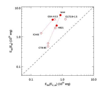
Figure 5: Comparison of supernova explosion energies calculated from kinetic energy of Hi(+H₂) shell ($E_{\rm SN}(E_{\rm K,\,sh})$) and thermal energy ($E_{\rm SN}(E_{\rm th})$). The symbols are same as Figure 4, i.e., Hi only (open circles) and Hi+H₂ (filled circles).

The comparison in Figures 2 and 4 showed that the observation-based global parameters of SNRs (i.e., $p_{\rm sh}$, $E_{\rm K,sh}$, and $E_{\rm th}$) are generally consistent with the 1D hydrodynamic simulations but at the same time that for most SNRs they cannot be explained by a single set of $E_{\rm SN}$ and $n_{\rm bg}$. One noticeable feature is that, for a given $n_{\rm bg}$, the SN explosion energy derived from thermal energy $E_{\rm SN}(E_{\rm th})$ is generally larger than those derived from momentum and kinetic energy of the shell, $E_{\rm SN}(p_{\rm sh})$ and $E_{\rm SN}(E_{\rm K,\,sh})$, while the latter two are almost comparable (Table 5; see also Figure 5). Five out of six SNRs with both $E_{\rm SN}(E_{\rm th})$ and $E_{\rm SN}(E_{\rm K,\,sh})$ estimated have $E_{\rm SN}(E_{\rm th})/E_{\rm SN}(E_{\rm K,\,sh})\geq 3$. In particular, for the two prototypical SNRs interacting with large MCs, i.e., W44 and IC 443, $E_{\rm SN}(E_{\rm th})/E_{\rm SN}(E_{\rm K,\,sh})$=6–8 when we adopt $\bar{n}_{\rm bg}$ corresponding to the density of the shocked Hi+H₂ gases averaged over the SNR volume.

There could be several possible explanations for the systematically larger $E_{\rm SN}(E_{\rm th})$ than $E_{\rm SN}(p_{\rm sh})$ and $E_{\rm SN}(E_{\rm K,\,sh})$. First, it could be due to a systematic error in deriving the global parameters from observation; the thermal energies could have been systematically overestimated or the shell momenta and kinetic energies could have been systematically underestimated. Thermal energies are derived by assuming that hot gas with a pressure determined from X-ray spectral analysis is filling the entire volume of an SNR. Considering that the X-ray parameters are often obtained from the analysis of X-ray bright regions in SNRs, this poses a large uncertainty in the derived thermal energy. If we had used the actual volume bright in X-rays, $E_{\rm SN}(E_{\rm th})$ could have been considerably smaller. For G54.4$-$0.3 that we analyzed in Appendix B.1, for example, the X-ray emission is filling an elliptical area of $38^{\prime}\times 22^{\prime}$, so that the thermal energy would be about 40% of $E_{\rm th}$ in Table 5 derived by assuming that the hot gas is filling the entire SNR. For IC 443, it has been proposed that the X-ray emitting plasma is confined to a thin shell (Troja et al., 2006), the volume of which is only a small fraction of the total volume of the SNR as should be the thermal energy. Small thermal energy would be more consistent with the observed momentum and kinetic energy of an SNR, but what fills the rest of the SNR volume needs to be explained. One possibility (M. Li et al, in preparation) is that the pressure of cosmic rays becomes important just inside the shell, helping to displace the hot gas inwards. The cosmic rays can be produced either in situ by the diffusive shock acceleration of thermal particles or by the compression/reacceleration of pre-existing cosmic rays. For the middle-aged SNRs interacting with dense MCs such as W44 and IC 443, it has been shown that the latter is sufficient to explain the radio and $\gamma$-ray emission of these SNRs (Uchiyama et al., 2010; Lee et al., 2015). In either case, radial expansion of gas in the SNR interior initially compresses and confines cosmic rays within the shell, they can subsequently move downstream into the SNR interior if the thermal pressure there drops below that of the shell.

Alternatively, the momentum and kinetic energy of the Hi shells could have been systematically underestimated. As was explained in § 2.1, the global parameters of the Hi shells are obtained from the thin-shell analysis of small, uncontaminated portion(s) of Hi 21 cm emission spectra. For some SNRs (W44, G54.4$-$0.3, HB21), we assumed that the shell is thin and expanding uniformly, so that the shell mass per unit LOS velocity is constant and the intrinsic Hi 21 cm profile is a rectangle. (The observed profile appears a flat-topped Gaussian because of the large turbulence velocity assumed, e.g., see Figure 9.) If there were more mass at low expansion velocities, the total mass and therefore the momentum and kinetic energy could have been underestimated. Since the expansion velocity of this low-velocity gas is small, however, its contribution to the derived kinetic energy (and momentum) might not be large (see § 4.2, however). The $E_{\rm SN}(E_{\rm th})$ substantially larger than the canonical SN explosion energy ($1\times 10^{51}$ erg) in these SNRs also suggests that the main reason for the inconsistency is probably not the underestimation of the shell kinetic energy, although careful analysis of SNR simulations in a realistic environment with mock observations is necessary to quantify the potential bias in the derivation of shell kinetic energy.

Another, probably more plausible, explanation for the systematic trend in Figure 5 might be that, in deriving SN explosion energy from the global parameters, it is difficult to take into account the complex environments of SNRs, and this is compounded by the parameter sensitivity of Equation 14 (and to a lesser extent Equation 12). As we already seen in many observed SNRs (e.g., Figure 1) and simulated SNRs (e.g., Figure 3), the real ISM provides a very complex environment to SNRs. In this case, the background medium density parameter $n_{\rm bg}$ in describing SNR evolution is not well defined. As demonstrated in 3D simulations considering inhomogeneous background medium (e.g., Figure 4; see also Kim & Ostriker 2015; Cho et al. 2015; Li et al. 2015; Martizzi et al. 2015; Walch & Naab 2015; Iffrig & Hennebelle 2015; Zhang & Chevalier 2019), fortunately, the evolutionary tracks of integrated quantities such as total momentum and kinetic energy in the radiative SNRs (i.e., after the shell formation) are not sensitive to the complexity of the background medium. In particular, the total momentum does not evolve in time after reaching a terminal value. The model uncertainty due to the ISM inhomogeneity is less than a factor of two. However, one single background medium density $n_{\rm bg}$ does not seem be applicable to both $E_{\rm SN}(E_{\rm th})$ and $E_{\rm SN}(E_{\rm K,\,sh})$. In our TS models, where the ambient medium has a large-scale non-uniformity, thermal energy is considerably smaller than that of the uniform medium case with the same mean density (Figure 4(e)). This also happens for some SNRs in TI models (see § 4.2). On the other hand, the observed thermal energies of the SNRs appear to be generally larger than those of the uniform medium cases with the same mean densities (Figure 4(f)). For the two prototypical SNRs interacting with MCs, W44 and IC 443, for example, Table 5 shows that $E_{\rm SN}(E_{\rm th})/E_{\rm SN}(E_{\rm K,\,sh})$=6–8 when we adopt the mean ambient density $n_{\rm bg}$(Hi+H₂)(=50–70 cm^-3). It is, however, clear that this density is much higher than the density of the material filling most of the volume of the ISM where the SN blast wave propagates. For example, the ambient density derived from an analysis of the X-ray surface brightness profile of W44 is $\sim 3$ cm^-3 (Harrus et al., 1997). An overestimated ambient density would predict a smaller $E_{\rm th}$ or a larger $E_{\rm SN}(E_{\rm th})$ to match the observed $E_{\rm th}$ (see Eq. 14). On the other hand, Eq. 14 is based on 1D simulations. In real SNRs in inhomogeneous/non-uniform medium, the cooling could be significantly enhanced due to the mixing and diffusion between the engulfed dense material and the hot plasma, in which case the thermal energy of real SNRs might be smaller than $E_{\rm th}$ predicted from 1D simulations. Therefore, it is not obvious if Equation 14 with $n_{\rm bg}$(Hi+H₂) would overpredict or underpredict $E_{\rm SN}(E_{\rm th})$ for SNRs in complex environments (see also § 4.2). High-resolution simulations of SNRs in realistic environments including the complex physics at the hot/cool interface are needed in oder to understand the environment dependency of the evolution of thermal energy.

It is worthwhile to point out that $E_{\rm SN}(p_{\rm sh})$ and $E_{\rm SN}(E_{\rm K,\,sh})$ in Table 5 were derived by assuming that the observed momentum and kinetic energy in Hi+H₂ dominate the total budget of momentum and kinetic energy of radiative SNRs, respectively. This might be a valid assumption for the majority of the SNRs studied in this paper. But it is still possible that some components of the momentum and kinetic energy are undetected (see also § 4.2). For example, the morphology of the SNR G54.4$-$0.3 suggests that the remnant is likely to be interacting with large MCs (Junkes et al., 1992a, b; Ranasinghe & Leahy, 2017), but only a small amount of shocked molecular gas has been detected. On the other hand, if an SN explodes in an environment with hot gas filling most of the volume (Li et al., 2015), the observed momentum of the atomic shell can significantly underestimate the total injected momentum because no radiative shell forms in the hot gas. For a more rigorous comparison of theory and observation, it needs to be investigated from numerical simulations how the momentum and kinetic and thermal energies are distributed in different phases of the ISM in different environments.

4.2 Uncertainties in the Thin Shell Analysis

The uncertainties in the derived global parameters of the SNRs are dominated by systematic uncertainties in analyzing the observed data. The measurement errors are small. Our basic assumption in the analysis was that the SNR is composed of a fast-expanding, spherical Hi shell and hot gas filling the interior. The shell is assumed to be geometrically ‘thin’ and the expansion velocity of the shell material is assumed to be either constant or varying radially depending on the observed properties of the Hi 21 cm emission (see § 2.1). The hot gas is assumed to have a constant pressure, although its density and temperature may not be uniform. We further assumed that all the SNR momentum resides in the shell (and possibly in shocked molecular gas in addition). The errors in the global parameters obtained from this thin-shell analysis might depend on the complexity of the environment, and it is difficult, if not impossible, to quantify the errors for individual SNRs. By comparing these observation-based global parameters with those obtained from the same analysis of mock observations from simulations of SNRs in realistic environments, we can in principle infer the environments of individual SNRs and/or we can validate theoretical SNR models. In this work, however, we compared the observation-based global parameters with the total momentum and total kinetic/thermal energy obtained from numerical simulations. We took this approach as the most practical for an initial study comparing theory and observations. Given the limitations of our approach, however, we consider it worthwhile in this section to estimate the uncertainties/errors in the comparison arising from applying the thin-shell analysis by using one of the TI model SNRs (KO15, see also § 3.2). The simulation was not intended to be compared in detail to any real SNR, but the result will be useful in understanding the systematic uncertainties in our analysis.

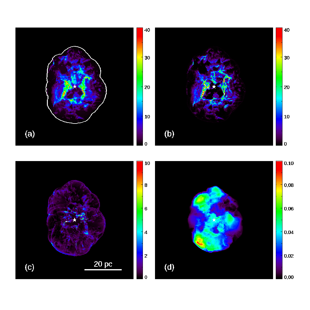
Figure 6: Projected hydrogen column densities of initial ambient medium and the SNR material: (a) initial ambient medium, (b) slow neutral component expanding at $v_{r}<50$ km s^-1, (c) fast neutral component expanding at $v_{r}\geq 50$ km s^-1, and (d) hot component with $T>5\times 10^{5}$ K. The SNR has been produced in a two phase ISM with $\bar{n}_{\rm bg}=10$ cm^-3, and it is $5\times 10^{4}$ yrs old (see § 4.2). In panel (a), we show the initial column density distribution (before the explosion) of material that is later shocked and joins the SNR. The white contour represents the projected outer boundary of the SNR. The scale in each frame is in units of $1\times 10^{20}$ cm^-2.

The simulated SNR is one out of the ten realizations with a mean density of the background medium $\bar{n}_{\rm bg}=10$ cm^-3 (purple lines in Figure 4; S2P-n10 model in Table 2 of KO15). The explosion energy was $E_{\rm SN}=10^{51}$ erg. We consider the background medium with high ambient density that is close to the environment of the middle aged SNRs such as W44 where we see a fast expanding Hi shell and also the shocked molecular gas (see below; see also Zhang & Chevalier 2019). The background medium consists of two distinct components; WNM and CNM with a mean density of 1.5 cm^-3 and 110 cm^-3, respectively (Figure 6). The WNM is filling most of the volume with the volume filling factor $f_{V,{\rm WNM}}=0.88$, while the CNM contributes most (83%) of the mass. For convenience, the velocity of the background medium was set to zero, so that the SNR material can be easily distinguishable by selecting either hot ($T\geq 2\times 10^{4}$ K) or dynamically-perturbed ($|v|\geq 1$ km s^-1) gas. We separate the SNR material into different components using temperature cuts; neutral ($T<2\times 10^{4}$ K), ionized ($2\times 10^{4}$  K $\leq T\leq$ $5\times 10^{5}$ K), and X-ray-emitting hot gas ($T>5\times 10^{5}$ K). The neutral includes potential molecular gas. The shell formation time of the WNM is $3.5\times 10^{4}$ yr (see Eq. 2), so we have chosen a snapshot at $5\times 10^{4}$ yr for our analysis. Figure 6 shows the spatial distribution of the neutral (in panels (b) and (c)) and hot (in panel (d)) components as well as that of the initial ambient medium (in panel (a)). The neutral is further divided into two components, (b) slow ($v_{r}<50$ km s^-1) and (c) fast ($v_{r}>50$ km s^-1), based on their expansion velocity (see below). The SNR has an ellipsoidal shape with radial distance from the explosion center to the boundary ranging from 15 pc to 21 pc. The volume-averaged mean radius is $R_{s,{\rm vol}}=16.5$ pc while the geometrical mean radius of the SNR projected on the sky ($x$-$y$ plane) is 17.8 pc.

The top frame in Figure 7 shows the mass distribution of the neutral component of the simulated SNR in radial velocity, i.e., $dM/dv_{r}$ where $v_{r}$ is radial velocity. It shows that $dM/dv_{r}$ decreases continuously with $v_{r}$, i.e., there is more mass at lower velocities, which is very different from what we expect for a thin shell expanding at a constant speed. This is because the background medium is composed of two distinct components, each of which has a range of densities. Most of the mass at high and low velocities are from the shocked WNM and the shocked CNM, respectively. The break in the slope of $dM/dv_{r}$ at $v_{r}\sim 50$ km s^-1 suggests that the predominance of the two components switches across this velocity. This is more clearly seen in the momentum distribution $dp/dv_{r}$ (Figure 7 middle frame), where we see that $dp/dv_{r}$ has a Gaussian-like distribution at $v_{r}\lower 2.15277pt\hbox{$\;\buildrel<\over{\sim}\;$}50$ km s^-1, while it decreases linearly with $v_{r}$ at higher velocities. For convenience, we divide the neutral SNR gas into two components: the ‘slow’ component expanding at $v_{r}<50$ km s^-1 and the ‘fast’ component expanding at $v_{r}\geq 50$ km s^-1. We note that the hydrogen mass of the fast component is 500 $M_{\odot}$, which is comparable to the swept up mass of the WNM ($\approx(4\pi/3)f_{V,{\rm WNM}}R_{s,{\rm vol}}^{3}\approx 590$ $M_{\odot}$). Figure 6 shows the spatial distribution of the slow and fast components. As expected, the fast component is dominated by the expanding shell in the WNM with some additional mass in the interior, while the slow component is mostly the shocked dense CNM in the interior. One thing to notice is that the slow component is surrounding the explosion center. This is because the intial gas distribution is somewhat artificial in a sense that the CNM and WNM are isotropically distributed with respect to the SN, and their mass and volume fractions are solely set by thermal instability without realistic considerations of turbulence and magnetic fields in the ISM. The momenta of the two components are comparable while the kinetic energy of the fast component is three times greater than that of the slow component. Table 6 summarizes the physical parameters of the individual components of the SNR as well as those of the entire SNR.

We adopted $z$ axis as the LOS, and Figure 7 shows the mass distribution in the LOS velocity $dM/dv_{\rm LOS}$. The $dM/dv_{\rm LOS}$ is also composed of two distinct distributions corresponding to the slow (solid line) and fast (grey filled area) components. The fast component appears as a broad wing that extends to high LOS velocities, and the mass at $|v_{\rm LOS}|>50$ km s^-1 is entirely due to the fast component. Before we perform an Hi 21 cm line analysis of the simulated SNR, it is worthwhile to consider what we would or would not see in Hi 21 cm emission. The Hi 21 cm emission that has been detected in the SNRs in Table Radiative Supernova Remnants and Supernova Feedback are all at the highest LOS velocities (e.g., see Figure 9), which corresponds to the broad wing due to the fast neutral component in Figure 7. With turbulence, the slow neutral component with large expansion velocities can also have LOS velocities higher than 50 km s^-1, but its contribution to the detected Hi emission at the highest LOS velocities will be negligible. The Hi 21 cm line analysis, therefore, provides the parameters of the fast component or the expanding shell in the WNM, but it does not provide any information about the slow neutral component or the slowly expanding dense material in the interior.

We have produced a synthetic Hi 21 cm line profile of the simulated SNR as in Kim et al. (2014). We set the spin temperature of the neutral hydrogen ($T<2\times 10^{4}$ K) equal to the gas kinetic temperature, assuming efficient excitations by collisions in the CNM and Ly$\alpha$ resonant scattering in the WNM (Seon & Kim, 2020). Note that the Hi 21 cm line emission from the shocked SNR Hi gas is usually optically thin, so that the line intensity is just proportional to the column density at high velocities and the details of the excitation and/or radiative transfer are not an issue in deriving the Hi mass. Since we make the ambient medium static in the simulation, we add a turbulent velocity field to $v_{\rm LOS}$ to mimic random motions in the diffuse Hi. We generate a Gaussian random velocity field with a power-law slope of $-2$ in the wavenumber space and the rms amplitude is set to 10 km s^-1. We also add a white noise with an rms amplitude of 0.03 K to the brightness temperature for an instrumental noise.

The synthetic Hi 21 cm line spectrum of the SNR is shown in the top frame of Figure 8 where the dotted line is a background spectrum obtained from an annular ring surrounding the SNR. The middle frame shows the background-subtracted Hi spectrum where we see the excess emission associated with the SNR at velocities higher than $\pm 30$ km s^-1. In real SNRs, only the emission at the highest velocities are seen because the emission from the foreground/background Hi gas is very broad due to the Galactic rotation. We assume that either only the spectrum at $|v_{\rm LOS}|\geq 70$ km s^-1 or at $|v_{\rm LOS}|\geq 90$ km s^-1 is visible, and perform a least squares fitting to obtain the expansion velocity and the hydrogen column density, which are used to derive the age, mass, momentum, and kinetic energy of the shell (see § 2.1). For the radius of the SNR, we use the geometrical mean radius (17.8 pc) as it appears on the sky. For the expanding shell, we adopt the simplest thin shell model where the shell material is expanding at a constant speed. But the shell is assumed to be turbulent with a large ($\Delta v_{\rm FWHM}=50$ km s^-1) dispersion in the LOS velocity, so that the model Hi 21 cm spectrum appears as a flat-topped Gaussian. This velocity width is from the observation of Hi clumps in the expanding SNR shells and it is what had been used for the fit in previous studies (e.g., Park et al., 2013). The details of the fitting procedure may be found in Park et al. (2013) (see also Appendix A). The bottom frame of Figure 8 is zoom-in of the middle frame and shows the best fit profiles, and Table 7 summarizes the derived shell parameters.

Table 7 shows that the global parameters derived from the Hi 21 cm line analysis agree well with those of the fast component of the simulated SNR. When using only the Hi profile at the highest LOS velocities ($|v_{\rm LOS}|\geq 90$ km s^-1), the mass is substantially ($\lower 2.15277pt\hbox{$\;\buildrel>\over{\sim}\;$}30$%) underestimated. On the other hand, the derived expansion velocity is larger than the mass-weighted radial velocity of the SNR shell, so that the momentum and kinetic energy agree with those of the simulated SNR within $\sim 10$%. The age also agrees with the age of the simulated SNR. When the Hi profile at $|v_{\rm LOS}|\geq 70$ km s^-1 is used, the mass becomes larger, and the momentum and kinetic energy are overestimated by $\sim 20$%. So, for the simulated SNR analyzed in this section, the errors in the momentum and kinetic energy of the fast neutral component of the SNR arising from the thin-shell analysis are small ($\lower 2.15277pt\hbox{$\;\buildrel<\over{\sim}\;$}20$%). There is slowly-expanding neutral material inside SNR, which is not included in the analysis. Its momentum is slightly larger than that of the expanding shell while its kinetic energy is much less (Table 6). This slow neutral component is not likely to be traced by the Hi 21 cm line emission in the observations of real SNRs because of the background/foreground contamination. Hence, the comparison cannot be made. If the slow neutral component is molecular, however, it can be detected in molecular emission lines and can be included in the comparison as in the SNRs W44 and IC 443.

We can also estimate the error in the thermal energy arising from the thin-shell analysis. In the simulated SNR, the volume filling factor of the hot gas is 53%. The rest is filled with the neutral (28%) and the ionzied (19%). Hence, if we derive thermal energy assuming that the hot gas is filling the entire SNR having a spherical volume of radius $R_{\rm sh}$ (=17.8 pc), which is larger than the volume-averaged radius (16.5 pc), the thermal energy would be overestimated by a factor of 2.4.

If we naively accept the result of the above analysis, the momentum of the radiative ‘shell’ in Table 4 could be underestimated by as much as a factor of ($p_{\rm sh}$(Hi)+$p_{\rm sh}$(H₂))/(2$p_{\rm sh}$(Hi)+$p_{\rm sh}($H₂)) because the slow component is not included. If the shocked molecular gas fully accounts for the slow component, however, the error is small ($\lower 2.15277pt\hbox{$\;\buildrel<\over{\sim}\;$}20$%). The error in the kinetic energy due to the missing slow component is small ($\lower 2.15277pt\hbox{$\;\buildrel<\over{\sim}\;$}30$%). Thermal energy could be overestimated by a factor of 2–3 due to the geometrical uncertainty. The error in the age of the shell appears to be small.

Finally, we estimate the error in the derived explosion energy from the “observed” global parameters of the simulated SNR. Table 8 shows $E_{\rm SN}$ obtained from the parameters of the $|v_{\rm LOS}|\geq 70$ km s^-1 case in Table 7. (The results are essentially the same for $|v_{\rm LOS}|\geq 90$ km s^-1.) With the background density $\bar{n}_{\rm bg}=0.90{\rm\,cm^{-3}}$, we obtain $E_{\rm SN}(p_{\rm sh})\approx E_{\rm SN}(E_{\rm K,\,sh})\approx 0.23\times 10^{51}$ erg, i.e., the derived explosion energy from the momentum and kinetic energy of the shell is consistently lower by about a factor of 4. We also show the results in a hypothetical case when the slow component ($|v_{r}|<50$ km s^-1; Table 6) is observed, e.g., in molecular lines, and its mass, momentum, and kinetic energy are included in the analysis. (Note that this corresponds to the Hi+H₂ case in Table 5.) In principle, $E_{\rm SN}$ should be close to 1 in the latter case, but because the analytic evolution tracks are generally above the evolution tracks of the TI models (see Figure 4), $E_{\rm SN}(p_{\rm sh})$ and $E_{\rm SN}(E_{\rm K,\,sh})$ are underestimated by a factor of 2. Therefore, actual bias introduced by the missing slow component is a factor of 2 underestimation in the derived explosion energy. For $E_{\rm SN}(E_{\rm th})$, we use $E_{\rm th}=4.2\times 10^{49}$ erg, which is 2.4 times the thermal energy of the hot gas (see the above paragraph). We obtain $E_{\rm SN}(E_{\rm th})=0.17\times 10^{51}$ erg for $n_{\rm bg}=0.90{\rm\,cm^{-3}}$ and $E_{\rm SN}(E_{\rm th})=0.63\times 10^{51}$ erg for $n_{\rm bg}=6.7{\rm\,cm^{-3}}$. Note that $E_{\rm SN}(E_{\rm th})$ is underestimated, although $E_{\rm th}$ has been overestimated. This is again because the analytic evolution track is above the evolution tracks of the TI models (Figure 4); thermal energy of the simulated SNR drops rapidly after the shell formation, so that $E_{\rm SN}(E_{\rm th})$ derived from the analytic evolution track is underestimated by a factor of 3. Therefore, actual bias introduced by the geometrical uncertainty is a factor of 2 ($=3\times 0.63$) overestimation in the derived explosion energy. If the slow component is not included ($n_{\rm bg}=0.90{\rm\,cm^{-3}}$), $E_{\rm SN}(E_{\rm th})$ is underestimated by a factor of 2 ($=1/(3\times 0.17)$) because of the low background density (see Eq. 14). Hence, aside from the uncertainties associated with the analytic evolution tracks, $E_{\rm SN}(E_{\rm th})$, as well as $E_{\rm SN}(p_{\rm sh})$ and $E_{\rm SN}(E_{\rm K,\,sh})$, in Table 5 would be underestimated by a factor of 2 due to the missing slow component. For $E_{\rm SN}$ obtained with the background density of Hi+H₂, if the shocked molecular gas corresponds to the slow component, $E_{\rm SN}(E_{\rm th})$ would be overestimated by a factor of 2 due to geometrical uncertainty, while the errors in $E_{\rm SN}(p_{\rm sh})$ and $E_{\rm SN}(E_{\rm K,\,sh})$ might be small.

How general is the above result? It has been shown that total momentum/kinetic energy of the SNRs in simulations after shell formation differs by less than a factor of 2 in a wide variety of background conditions (see § 3.2). The relative distribution in different phases of the ISM, however, could be very different depending on the environment as well as the age of the SNR. On the other hand, it does not seem unreasonable to expect that the SNRs of similar ages with fast expanding Hi shells detected have similar environments. For example, if the ambient medium is rarefied the Hi shell will not be formed until the SNR becomes very old (e.g., $\lower 2.15277pt\hbox{$\;\buildrel>\over{\sim}\;$}10^{5}$ yr when $\lower 2.15277pt\hbox{$\;\buildrel<\over{\sim}\;$}0.1$ cm^-3; Eq. 2). Or, if the ambient medium is dense, the Hi shell will be detected only for relatively young SNRs because the expansion velocity of the Hi shell will drop below the detection limit in the early stages of their evolution. Hence, the parameter space to be searched is likely to be restricted. We consider that the thermal energy content of hot gas might be important in exploring the parameter space. As we mentioned in § 3.2, the thermal energy evolution of radiative SNRs is sensitive to the structure of the background medium. Indeed the thermal energy of the hot gas in the simulated SNR ($1.7\times 10^{49}$ erg) is more than a factor of 4 smaller than the thermal energy predicted from Equation 14 which is $7.4\times 10^{49}$ erg. This suggests that the discrepancy in thermal energies found in § 3.2 could be environmental, although, as we have seen in the simulated SNR, the thermal energies obtained by assuming a spherical volume filled with hot gas could have been overestimated by a factor of 2–3. Owing to many simplifications made to obtain the initial ambient medium and some missing physics in the simulated SNR as well as the simplifications in creating the mock observation (see § 4.3), the current analysis should be considered as one case study to understand the potential errors in comparing the observation-based global parameters with simulations. It will be interesting to look into the momentum contribution from the slow neutral component and the thermal energy issue with realistic simulations and in a wider parameter space in future works.

4.3 Missing Physics in Numerical Models

There are a few physics elements missing in the three-dimensional simulations presented here, including thermal conduction and cosmic rays as well as magnetic fields. The role of the interstellar magnetic fields has been briefly investigated in KO15, demonstrating that magnetic fields that are stronger than $B\sim 7\ \mu{\rm G}$ can alter the shape of an SNR and reduce the late time momentum slightly as the shell expands back to the interior due to strong magnetic pressure built in the shell. Yet, the reduction is slight, well within the uncertainty we consider here.

Thermal conduction transfers energy from the interior to the shell, which is compensated by energy delivered by flow from the shell due to evaporation. This effect is actually included in the one-dimensional simulations presented in this paper, using the same framework developed for superbubble evolution driven by multiple SNe in El-Badry et al. (2019). For a single SN, the evolution is almost identical without thermal conduction.

In the clumpy ISM, the role of thermal conduction can be enhanced and more generally termed as the effect of “mass loading”. As a result of interaction between blastwaves and embedded cold clouds, cold clouds are evaporated by thermal conduction (e.g., Cowie & McKee, 1977) and shredded by hydrodynamic instabilities (e.g., Klein et al., 1994). Then, the interior hot remnant loads more mass and cools more rapidly, altering the overall evolution of the integrated properties of SNRs. The “mass loading” effect is in part modeled in KO15 (and the TI models presented in Figure 4) as it explicitly simulates blast wave expansion within a clumpy medium, while the resolution requirement to resolve cloud crushing is more stringent (e.g., Schneider & Robertson, 2017). Slavin et al. (2017) and Zhang et al. (2019) conducted a set of 2D and 3D simulations for SNR expansion in cloudy medium with thermal conduction and modeled X-ray emission to explain the centrally-peaked X-ray in MM SNRs. Since radiative cooling is ignored in their simulations (adiabatic simulations), unfortunately, a direct link between X-ray emission and remaining thermal energy is not possible. Although the evolution is limited to a time shorter than the shell formation time of the background medium, blastwaves propagate into clouds as well as gas in the interface and wakes would have cooled. Zhang & Chevalier (2019) modeled a radiative SNR in a turbulent medium (without conduction) and showed that total energy and momentum evolution is not very sensitive to the Mach number of the medium. The interior X-ray emission has brightened in the turbulent medium, but not as bright as its adiabatic counterpart.

Besides full 3D simulations with explicit treatment of the inhomogeneous ISM, the effect of “mass loading” has been investigated using similarity solutions (e.g., McKee & Ostriker, 1977; White & Frenk, 1991) and one-dimensional simulations (e.g., Cowie et al., 1981; Pittard, 2019). Very recently, Pittard (2019) suggests that the final momentum can be reduced significantly by the mass loading from cold gas. However, even for the case with $f_{\rm ML}=100$, in which mass loaded by clouds is 100 times larger than the swept-up mass at the shell formation, the reduction of the final momentum is only 56%, which again well within the range of model uncertainty considered here. Furthermore, the mass loading generally enhances cooling so that the thermal energy of SNRs might be reduced compared to that without the mass loading, which would increase the discrepancy between the explosion energies inferred from thermal and momentum/kinetic energy. 3D simulations of a radiative SNR in a inhomogeneous medium with thermal conduction at high resolution will illuminate the role of mass loading in dynamical evolution and observational signatures of MM SNRs.

The last piece of the puzzle in SNR evolution study is the role of cosmic rays. It is well accepted that blastwave shocks are the main source of energetic particles (e.g., Bell, 1978; Blandford & Ostriker, 1978). As cosmic ray energy is $\sim 10-20\%$ of kinetic energy of SN ejecta (e.g., Caprioli & Spitkovsky, 2014; Park et al., 2015) and hardly radiated away, cosmic ray pressure can be a source of further acceleration in the pressure-driven snowplow phase if cosmic rays are confined preferentially behind the shell. Recent semi-analytic analysis suggests that the final momentum deposition can be enhanced by more than a factor of 5 with $E_{\rm CR}\sim 0.1E_{\rm SN}$ (Diesing & Caprioli, 2018). However, the efficiency of cosmic ray momentum boost depends strongly on the evolving spatial distribution of cosmic rays relative to the gas concentrated in the shell, which depends on cosmic ray streaming and diffusion (M. Li et al. 2020 in prep.). Therefore, the impact of cosmic rays on SNR evolution is uncertain yet and an active area of research.

Overall, the theoretical uncertainty from numerical studies in describing the evolution of momentum and kinetic energy of radiative SNRs is less than a factor of two for commonly explored physics (e.g., magnetic fields, background medium inhomogeneity and turbulence, thermal conduction) unless cosmic rays significantly alter the momentum deposition in the high density medium. This allows us to derive the explosion energy relatively reliably from momentum and kinetic energy of radiative SNRs if the observed momentum and kinetic energy are the majority. As discussed in Section 4.2, uncertainties at the level of a factor $\sim 2$–4 can arise from applying the thin, spherical shell model together with analytic evolution tracks to Hi emission lines in order to estimate momentum and kinetic energy, or infer the explosion energy. On the other hand, the thermal energy evolution of the radiative SNR is sensitive to the density of the surrounding medium, giving rise to a large model uncertainty in thermal energy and the derived explosion energy.

5 Conclusion

Supernova explosions control the evolution of the ISM and galaxies by injecting prodigious energy and momentum. The energy produces the hot phase of the ISM, while the momentum drives turbulence and regulates the star formation. To understand the ISM structure and evolution of galaxies, therefore, it is important to ‘quantify’ the SN feedback, particularly the momentum transferred to the ISM and the amount of hot gas created during the lifetime of an SNR. There have been several 3D numerical simulations for such purpose (e.g., KO15; Li et al., 2015; Martizzi et al., 2015; Walch & Naab, 2015; Iffrig & Hennebelle, 2015; Zhang & Chevalier, 2019). According to these numerical studies, the radial momentum and kinetic energy of SNRs are insensitive to the density structure of the ISM, so that they are only slightly ($\lower 2.15277pt\hbox{$\;\buildrel<\over{\sim}\;$}50\%$) different from those in a uniform medium of the same mean density. The final momentum injected to the ISM by a single SN explosion is $p_{\rm sh}=(1-5)\times 10^{5}$ $M_{\odot}$km s^-1. Observationally, however, it is very difficult to detect radiative shells associated with SNRs because of the contamination due to the background/foreground Hi emission. So there are only a limited number of SNRs with radiative expanding shells detected and, even in those SNRs, we are not seeing all of the shell material but only the fastest expanding portion of the shell. In previous studies, the parameters of the expanding shells have been derived from the thin-shell analysis of Hi 21 cm emission line data. In this study, for seven radiative SNRs with fast expanding Hi shells, we have inventoried their shell parameters and also their thermal energies and the parameters of the shocked molecular gas associated with the SNRs, and compared them with the results of 1D and 3D numerical simulations in realistic environments. We also carried out a mock observation of a simulated SNR and discussed the uncertainties/difficulties in the comparison. In the following we summarize the main results of this work:

1. We provide a table (Table Radiative Supernova Remnants and Supernova Feedback) summarizing the global parameters of radiative Hi shells in the seven SNRs obtained from the thin-shell analysis of Hi 21 cm emission line data. All parameters are from the literature except those of HB 21 which are derived in this paper. The momentum, kinetic energy, and the age of the SNRs are in the range of $p_{\rm sh}=(0.5$–$4.5)\times 10^{5}$ $M_{\odot}$ km s^-1, $E_{\rm K,sh}=(0.4$–$3.5)\times 10^{50}$ erg, and $t_{\rm sh}=(0.3$–$3.4)\times 10^{5}$ yr, respectively.

2. Among the seven SNRs, four SNRs are known to be interacting with MCs (see Table Radiative Supernova Remnants and Supernova Feedback). In W44 and IC 443, the momentum of shocked molecular gas is comparable to or even larger than that of the Hi shell (1.8 and $0.7\times 10^{5}$ $M_{\odot}$ km s^-1), while its kinetic energy is relatively small ($\lower 2.15277pt\hbox{$\;\buildrel<\over{\sim}\;$}0.2\times 10^{50}$ erg). In the other SNRs, the shocked molecular gas is either not prominent or has not been detected, so that the momentum and kinetic energy of shocked molecular gas might not be significant.

3. Table 4 summarizes the global parameters of the seven SNRs. The total (atomic+molecular) momentum and kinetic energy of the SNRs are in the range of $p_{\rm sh}=$(1.1–4.5)$\times 10^{5}$ $M_{\odot}$ km s^-1 and $E_{\rm K,sh}=$(0.6–3.5)$\times 10^{50}$ erg, respectively. The table also lists the thermal energies of the SNRs (see also Table Radiative Supernova Remnants and Supernova Feedback). They are from the literature except those of G54.4$-$0.3 and CTB 80 which are derived in this work. The thermal energy, assuming that the interior of the SNR is filled with hot gas, is in the range of $E_{\rm th}=(0.6-8)\times 10^{50}$ erg.

4. The observation-based global parameters of SNRs are generally consistent with the 1D hydrodynamic simulations. In particular, the momenta of seven SNRs are all very close to the expected terminal values based on numerical models for the canonical SN explosion energy of $10^{51}~{}{\rm erg}$. By comparing with a variety of 3D hydrodynamic simulations with different background medium states, we show that the systematic uncertainty in determining the explosion energy is less than a factor of 2 for momentum and kinetic energy. Modulo systematic uncertainties in the global parameters, our inferred explosion energy (Table 5) is consistent with $10^{51}{\rm\,erg}$. Thermal energy, however, depends strongly on the density structure of the background medium, so that a single mean density of the background medium in general cannot be used to characterize both thermal and kinetic energies.

5. We explored the uncertainties arising from applying the thin-shell analysis by using a mock Hi observation of a simulated SNR in the two phase ISM. It shows that there could be dense, slowly-expanding neutral material unseen in Hi emission and hence not included in the thin-shell analysis unless it is molecular. In the simulated SNR, this slow neutral component has a substantial volume filling factor and its momentum is comparable to that of the fast expanding Hi shell. The result might depend on the environment as well as the SNR age, and it needs to be investigated from numerical simulations how the momentum and kinetic/thermal energy are distributed in different phases of the ISM in different environments.

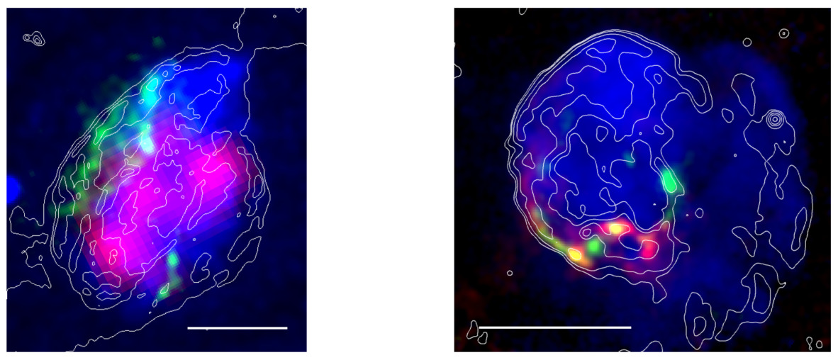
Figure 1: Two prototypical SNRs with both shocked atomic and shocked molecular gases: W44 (left) and IC 443 (right). North is up and east is to the left. Red=shocked atomic gas in Hi 21 cm emission (W44: Park et al. 2013 , IC443: Lee et al. 2008), Green=shocked molecular gas in HCO⁺ J=1–0 line (W44: Sashida et al. 2013, IC443: Lee et al. 2012), Blue=shocked hot gas in X-ray from Chandra (W44: Rho et al. 1994, IC443: Asaoka & Aschenbach 1994), Contour=21 cm continuum (W44: Giacani et al. 1997, IC 443: Lee et al. 2008). The scale bar in each frame represents 10 pc at the assumed distance of the SNR (see Table Radiative Supernova Remnants and Supernova Feedback).

Figure 7: Mass and momentum distribution of neural gas in the simulated SNR in velocity: mass distribution in radial velocity (top), momentum distribution in radial velocity (middle), and mass distribution in LOS velocity (bottom). The filled area in the bottom frame shows the distribution of the fast ($v_{r}\geq 50$ km s^-1) neutral component.

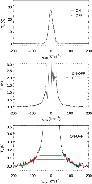
Figure 8: Top: Source and background Hi 21 cm profiles of the simulated SNR. The source profile is the average profile inside the circular area of radius 20 pc, while the background profile is the average profile inside the annulus of inner and outer radii of $22$ pc and $24$ pc, respectively. Middle: Background-subtracted Hi spectrum (solid line). Bottom: A close-up view of the background-subtracted Hi spectrum and a fit. The two red solid lines are the best fits to the profile at $|v_{\rm LOS}|>70$ km s^-1 and 90 km s^-1, respectively (see text).

Table 1: Parameters of Radiative HI Shells Associated with SNRs

G-name	Name	d	$v_{0}$	$R_{\rm sh}$		$v_{\rm sh}$	$t_{\rm sh}$		$M_{\rm sh}$(Hi)	$p_{\rm sh}$	$E_{\rm K,sh}$	Ref.
		(kpc)	(km s-1)	(pc)		(km s-1)	($10^{4}$ yr)		($10^{3}~{}M_{\odot}$)	($10^{5}$ M⊙ km s-1)	($10^{50}$ erg)
G34.7$-$0.4	W44	2.8	47	12.5	135(2)	2.7	0.39(0	0.74(0.03)	1.0(0.04)	1
G54.4$-$0.3		6.6	37	38.4	62(6)	18	2.3(0	2.0(0.6)	1.3(0.4)	1,2
G69.0+2.7	CTB80	2	13	19	72(3)	7.7	1.1(0	1.1(0.2)	0.76(0.16)	1
G89.0+4.7	HB 21	1.7	$-12$	26	61(4)	13	2.2(0	1.9(0.4)	1.2(0.3)	this work
G189.1+3.0	IC 443	1.5	$-5$	7.1	75(8)	2.8	0.49(0	0.52(0.08)	0.39(0.09)	3, 4
G172.8+1.5	$\cdots$	1.8	$-20$	61	55(5)	33	5.9(0	4.5(0.7)	2.5(0.6)	5
G190.2+1.1	$\cdots$	8	20	88	77(6)	34	4.2(0	4.5(1.0)	3.5(0.9)	6

Note. — $d,v_{0}=$ distance and systemic velocity of SNR; $R_{\rm sh},v_{\rm sh}=$ radius and expansion velocity of Hi shell; $t_{\rm sh}(\equiv 0.3R_{\rm sh}/v_{\rm sh})=$ characteristic age of Hi shell; $M_{\rm sh}$(Hi)= Hi mass of shell; $p_{\rm sh},E_{\rm K,sh}=$ momentum and kinetic energy of Hi shell including the contribution from He assuming cosmic abundance. The errors in parentheses are $1\sigma$ errors from least-squares fits except the error of the expansion velocity of IC 443 which gives a dispersion in the shock speed (see Fig. 11 of Alarie & Drissen 2019). The mass, momentum, and kinetic energy are derived from the thin-shell analysis, and their uncertainties are dominated by systematic uncertainties in analyzing the observed data (see § 4.2). Distances are the same as those used in the references except for G54.4$-$0.3 and HB 21. For G54.4$-$0.3, we adopt the ‘far’ distance 6.6 kpc corresponding to $v_{0}=37$ km s^-1 of Ranasinghe & Leahy (2017), which is consistent with the large H column density to the the source obtained from our X-ray analysis (see Appendix B.2). For HB 21, we adopt 1.7 kpc following Byun et al. (2006).

References. — (1) Park et al. (2013); (2) Ranasinghe & Leahy (2017); (3) Lee et al. (2008); (4) Alarie & Drissen (2019); (5) Kang et al. (2012); (6) Koo et al. (2006)

Table 2: Parameters of Shocked Molecular Gas in Radiative SNRs with HI Shells

Name	$M_{\rm sh}$(H2)	$v_{\rm sh}$	$p_{\rm sh}$		$E_{\rm K,sh}$		Tracer	Ref.
	($10^{3}~{}M_{\odot}$)	(km s-1)	($10^{5}$ M⊙ km s-1)		($10^{50}$ erg)
W44	10(5)	12.9(0.2)	1.8(0	0.23(0.12)	HCO+ $J$=1–0, CO $J$=3–2	1
G54.4$-$0.3	…	…	.	…	.	…
CTB80	…	…	.	…	.	…
HB 21	0.73	$\sim 10$	0.16	0.034	CO $J$=1–0, 2–1	2, 3
IC 443	2	25	0.7	0.17	HCO+ J=1–0	4
G172.8+1.5	…	…	.	…	.	…
G190.2+1.1	…	…	.	…	.	…

Note. — $M_{\rm sh}$(H₂)= H₂ mass of shocked molecular gas; $v_{\rm sh}=$ expansion velocity of molecular shell; $p_{\rm sh},E_{\rm K,sh}=$ momentum and kinetic energy of shocked molecular gas including the contribution from He assuming cosmic abundance. The errors in $M_{\rm sh}$(H₂) and $v_{\rm sh}$ of W44 are from Sashida et al. (2013). For HB 21 and IC 443, the errors are not given in References.

Note. — Comments on Individual Sources: W44: Sashida et al. (2013) divided the kinetic energy of shocked molecular gas into two terms corresponding to expansion and turbulent energies. The quoted $p_{\rm sh}$ and $E_{\rm K,sh}$ are those of the expansion motion. G54.4$-$0.3: There are MCs along the SNR shell (Junkes et al., 1992a, b; Ranasinghe & Leahy, 2017). Junkes et al. (1992a) derived the total mass of (1.3–2.6)$\times 10^{5}$ $M_{\odot}$ for these MCs and proposed that they form a large ($42^{\prime}$ or 86 pc at 7 kpc) molecular shell expanding at 5 km s^-1. There is, however, no convincing evidence for this. Instead, thin H₂ 2.122 $\mu$m emission filaments have been detected towards a small ($\sim 5^{\prime}$), radio-enhanced area in the western SNR shell (Lee et al. 2019; see also Fig 10). The total H₂ 2.122 $\mu$m luminosity ($6.4$ $L_{\odot}$) is 4% of that of W44, implying a small amount of shocked H₂ gas. CTB 80: There are extended filamentary MCs superposed on the SNR, but there is no evidence for the interaction between the SNR and the MCs (Koo et al., 1993). HB 21: Several small shocked MCs have been detected (Koo et al., 2001; Byun et al., 2006). The listed $M({\rm H}_{2})$, $p_{\rm sh}$, and $E_{\rm K,sh}$ are the sum of their masses, momenta, and kinetic energies, respectively. The systemic LOS velocities of these MCs are in the range of a few to 20 km s^-1, and the listed $\sim 10$ km s^-1 is a characteristic expansion velocity. IC 443: Both the shocked Hi and H₂ gases are mostly confined to an extended partial shell in the southern area (see Figure 1). G172.8+1.5: There are MCs in this area, but there is no evidence for the interaction between the SNR and the MCs (Kang et al. 2012; see also Dewangan et al. 2018). G190.2+1.1: MCs can be seen around the SNR in the CfA CO survey (Dame et al., 2001), but there is no evidence for the interaction.

References. — (1) Sashida et al. (2013); (2) Koo et al. (2001); (3) Byun et al. (2006); (4) Dickman et al. (1992)

Table 3: Parameters of X-ray Emitting Hot Gas in Radiative SNRs with HI Shells

Name	$\bar{n}_{e}$	$T$	$E_{\rm th}$	Ref.
	(cm-3)	(keV)	($10^{50}$ erg)
W44	0.36	0.88	3.7	1
G54.4$-$0.3	0.07	0.36	8.3	this work
CTB 80	0.08	0.18	0.6	this work
HB 21	0.03	0.66	2.4	2
IC 443	0.8–2.5	0.29–0.64	1.8	3
G172.8+1.5	$6\times 10^{-3}$	0.7	5	4
G190.2+1.1	$\cdots$	$\cdots$	$\cdots$	$\cdots$

Note. — $\bar{n}_{e},T=$ average electron density and temperature of X-ray emitting hot gas; $E_{\rm th}=$ thermal energy derived by assuming that hot gas in pressure equilibrium is filling the spherical volume of the SNRs.

Note. — Comments on Individual Sources: W44: Centrally-peaked diffuse X-ray emission is filling the interior of the SNR. The parameter $\bar{n}_{e}$ is obtained by assuming that the observed $EM$ ($1.8\times 10^{58}$ cm^-3, Harrus et al. 1997) is from an ellipsoidal volume of radii $27\times 16\times 25$ pc³. G54.4$-$0.3: Faint diffuse X-ray emission is filling the central area of the radio SNR. The parameters are derived in this work using the archival ASCA GIS data (see Appendix B.1). CTB 80: Faint X-ray emission of non-uniform brightness is filling the interior of the SNR shell. The parameters are derived in this work using the archival ROSAT PSPC data (see Appendix C). HB 21: Diffuse, centrally-brightened X-ray emission is filling the interior of the SNR. The parameter $\bar{n}_{e}$ is obtained by assuming that the observed $EM$ ($1.5\times 10^{56}$ cm^-3, Pannuti et al. 2010) is from a cylindrical volume with an angular radius $11\hbox{$.\mkern-4.0mu^{\prime}$}5$ and a path length $104^{\prime}$. IC 443: Bright X-ray emission is filling the northeastern area of the SNR with a faint emission extended to the southwest (Figure 1). The parameters $(\bar{n}_{e},T)$ are those of the ‘cold’ component of Troja et al. (2006), which has been proposed to be the shock-heated ambient medium. They assumed that this component is confined to two hemispherical thin (1 pc) shells; eastern shell of radius 7 pc (Shell A) and a western shell of radius 11 pc (Shell B) (see their Fig. 9). According to their result, the electron densities of Shell A and Shell B are $\sim 2$ cm^-3 and $\sim 1$ cm^-3, respectively, while their temperatures are both about 0.3 keV. We derived the thermal energy of the SNR by assuming that the inner volumes of Shell A and Shell B are filled with hot gas in pressure equilibrium at $\bar{n}_{e}T\sim 0.6$ cm^-3 keV and $\bar{n}_{e}T\sim 0.3$ cm^-3 keV, respectively. G172.8+1.5: Faint extended X-ray emission is visible superposed on the SNR in the ROSAT Survey Diffuse X-ray Background Map (Snowden et al., 1997). The listed parameter values are crude estimates derived from the broad-band counts assuming that the hot gas is uniformly filling the interior of the SNR (Kang et al., 2012). Here we assume $n_{e}=1.2n_{\rm H}$ and $E_{\rm th}\sim 3\bar{n}_{e}kTV$, and the numbers are sligthly different from those of Kang et al. (2012). G190.2+1.1: The SNR is not visible in the ROSAT all sky X-ray images (Koo et al., 2006).

References. — (1) Harrus et al. (1997); (2) Pannuti et al. (2010); (3) Troja et al. (2006); (4) Kang et al. (2012)

Table 4: Global Parameters of Radiative SNRs with HI Shells

Name	$\bar{n}_{\rm bg}$		$p_{\rm sh}$			$E_{\rm K,sh}$			$E_{\rm th}$
	(cm-3)		($10^{5}$ M⊙ km s-1)			($10^{50}$ erg)			($10^{50}$ erg)
	Hi	Hi+H2	Hi	H2	Hi+H2	Hi	H2	Hi+H2
W44	1.9	51	0.74	1.8	2.54	1.0	0.23	1.23	3.8
G54.4$-$0.3	0.4	0.4	2.0	$\cdots$	2.0	1.3	$\cdots$	1.3	8.3
CTB80	1.5	1.5	1.1	$\cdots$	1.1	0.76	$\cdots$	0.76	0.6
HB 21	1.2	1.6	1.9	0.1	2.0	1.2	0.01	1.21	2.4
IC 443	13	67	0.52	0.7	1.22	0.39	0.17	0.56	1.8
G172.8+1.5	0.25	0.25	4.5	$\cdots$	4.5	2.5	$\cdots$	2.5	5
G190.2+1.1	0.06	0.06	4.5	$\cdots$	4.5	3.5	$\cdots$	3.5	$\cdots$

Note. — $\bar{n}_{\rm bg}$ = $M_{\rm sh}$(Hi)$/m_{\rm H}V_{\rm sh}$ and $(M_{\rm sh}$(Hi)$+M({\rm H}_{2}))/m_{\rm H}V_{\rm sh}$ where $m_{\rm H}$ is the mass of H atom and $V_{\rm sh}=4\pi R_{\rm sh}^{3}/3$ (Note that these are not necessarily equal to the mean density of the ambient medium for SNRs in complex environment. See text.); $p_{\rm sh}$ = momentum of the atomic (Hi), molecular (H₂), and atomic+molecular (Hi+H₂) SNR shell; $E_{\rm K,sh}$ = kinetic energy of the atomic (Hi), molecular (H₂), and atomic+molecular (Hi+H₂) SNR shell; $E_{\rm th}$ = thermal energy of SNR from X-ray observation (see Tables Radiative Supernova Remnants and Supernova Feedback–Radiative Supernova Remnants and Supernova Feedback).

Table 5: Summary of Explosion Energy

Name	$\bar{n}_{\rm bg}$	$E_{\rm SN}(p_{\rm sh})$	$E_{\rm SN}(E_{\rm K,\,sh})$	$E_{\rm SN}(E_{\rm th})$
	(cm-3)	($10^{51}$ erg)
W44	1.9	0.32	0.35	0.63
	51 (Hi+H2)	1.37	0.87	5.26
G54.4-0.3	0.40	0.58	0.57	3.80
CTB80	1.5	0.35	0.35	0.47
HB21	1.2	0.61	0.61	2.01
	1.6 (Hi+H2)	0.66	0.67	2.42
IC443	13	0.21	0.21	1.30
	67 (Hi+H2)	0.62	0.49	3.69
G172.8+1.5	0.25	1.27	1.26	3.84
G190.2+1.1	0.06	1.22	1.25	$\cdots$

Note. — $\bar{n}_{\rm bg}$ = number density of hydrogen nuclei derived from observation either Hi only or Hi+ H₂ (see Table Radiative Supernova Remnants and Supernova Feedback); $E_{\rm SN}(p_{\rm sh})$, $E_{\rm SN}(E_{\rm K,\,sh})$, and $E_{\rm SN}(E_{\rm th})$ = SN explosion energy to match the observed $p_{\rm sh}$, $E_{\rm K,sh}$, and $E_{\rm th}$, respectively.

Table 6: Physical Parameters of the Simulated SNR

Parameter	Entire SNR	Neutral		Ionized	Hot
		$v_{r}<50$ km s-1	$v_{r}\geq 50$ km s-1
Age (yr)	$5\times 10^{4}$	$\cdots$	$\cdots$	$\cdots$	$\cdots$
$\bar{n}_{\rm bg}({\rm H})$ (cm-3)	8.5	$\cdots$	$\cdots$	$\cdots$	$\cdots$
$R_{s,{\rm vol}}$ (pc)	16.5	$\cdots$	$\cdots$	$\cdots$	$\cdots$
$M_{\rm H}(M_{\odot})$	$3.81\times 10^{3}$	$3.27\times 10^{3}$	496	29	19
Momentum $(10^{5}\ M_{\odot}\,{\rm km~{}s}^{-1})$	1.33	0.69	0.57	0.043	0.022
Kinetic energy ($10^{49}$ erg)	7.78	1.74	5.24	0.53	0.27
Thermal energy ($10^{49}$ erg)	2.03	$\cdots$	$\cdots$	0.29	1.74

Note. — $\bar{n}_{\rm bg}({\rm H})$ = average hydrogen density of the background medium swept-up by the SN blast wave. Note that it is a little smaller than $\bar{n}_{\rm bg}$ (=10 cm^-3) of the entire simulation box. $R_{s,{\rm vol}}$ = volume-averaged radius (i.e., volume = $(4\pi/3)R_{s,{\rm vol}}^{3}$). Momentum and kinetic energy include the contribution from He assuming the cosmic abundance of $n({\rm He})/n(\rm{H})=0.1$. Thermal energy is obtained from $E_{\rm th}=3\int n_{e}k_{B}T\,dV$ where $n_{e}=1.2n_{\rm H}$.

Table 7: Global Parameters of the Simulated SNR from Hi 21 cm Line Analysis

Parameter	Simulated SNR	Hi 21 cm line analysis
	$v_{r}\geq 50$ km s-1	$|v_{\rm LOS}|\geq 70$ km s-1	$\geq 90$ km s-1
Age (yr)	$5\times 10^{4}$	$5.5\times 10^{4}$	$4.7\times 10^{4}$
$R_{\rm sh}$ (pc)	16.5	17.8	17.8
H mass ($M_{\odot}$)	496	513(63)	330(78)
$\bar{n}_{\rm bg}$ (cm-3)	1.1	0.90(0.11)	0.57(0.21)
$\bar{v}_{\rm exp}$	82	94(6)	112(6)
Momentum $(10^{4}\ M_{\odot}~{}{\rm km}\,{\rm s}^{-1})$	5.73	6.8(0.9)	5.1(1.3)
Kinetic Energy $(10^{49}\ {\rm erg})$	5.24	6.3(1.1)	5.7(1.5)

Note. — The global parameters derived from an Hi analysis have been compared with those of the fast ($v_{r}\geq 50$ km s^-1) neutral component of the simulated SNR. The two columns in the Hi 21 cm line analysis show the parameters obtained from a fit to the profiles at $|v_{\rm LOS}|\geq 70$ km s^-1 and $|v_{\rm LOS}|\geq 90$ km s^-1 (see Figure 8), respectively. The velocity $\bar{v}_{\rm exp}$ of the simulated SNR is the mass-weighted average radial velocity. Momentum and kinetic energy include the contribution from He assuming the cosmic abundance of $n({\rm He})/n(\rm{H})=0.1$. The errors in parenthesis are formal errors from the fit.

Table 8: Explosion Energy of the Simulated SNR from Hi 21 cm Line Analysis

Hi 21 cm Line Analysis	$\bar{n}_{\rm bg}$	$E_{\rm SN}(p_{\rm sh})$	$E_{\rm SN}(E_{\rm K,sh})$	$E_{\rm SN}(E_{\rm th})$
	(cm-3)	($10^{51}$ erg)
$|v_{\rm LOS}|\geq 70$ km s-1	0.90	0.23	0.23	0.17
$|v_{\rm LOS}|\geq 70$ km s-1+ Slow component	6.7	0.54	0.47	0.63

Note. — The first row shows the results when we use the parameters of the Hi shell derived from the analysis of the Hi profile at $|v_{\rm LOS}|\geq 70$ km s^-1 in Table 7. The second row show the results when the slow component ($|v_{r}<50$ km s^-1) has been detected, e.g., in molecular lines, and their momentum and kinetic energy in Table 6 are included in addition to those of the Hi shell. (See text for more details.)

Appendix A Physical Parameters of the Expanding Hi Shell in HB 21

In this Appendix, we derive the parameters of the Hi shell associated with the SNR HB 21 (G89.0+4.7). HB 21 is an old SNR with an irregular radio shell of large angular size ($120^{\prime}\times 90^{\prime}$; see Figure 9). An expanding Hi shell associated with the SNR was detected by Koo & Heiles (1991) using the Hat Creek 85 foot telescope (FWHM=$36^{\prime}$). They detected high-velocity gas moving at $v_{\rm LSR}=40$ to 120 km s^-1 in the southern part of the SNR and derived the parameters of an expanding shell matching the observed Hi 21 cm line emission properties. We use the data from the HI4PI (HI4PI Collaboration et al., 2016) and the Leiden/Argentine/Bonn (LAB; Kalberla et al. 2005 Hi 21 cm line all-sky surveys. The HI4PI survey, which has been constructed from the Galactic All-Sky Survey (GASS) and the Effelsberg-Bonn HI Survey (EBHIS), provides a higher resolution ($16\hbox{$.\mkern-4.0mu^{\prime}$}2$) map with a comparable sensitivity ($1\sigma\sim 43$ mK). But as we will see below, the spectra appear to have baseline fluctuations at low-intensity level, so that we use the LAB survey data for quantitative analysis. The LAB survey combined three independent surveys of angular resolution of 30^′–36^′ to produce all-sky data at $0.\!\!^{\circ}5$ pixels with an rms noise of 0.07–0.09 K (Kalberla et al., 2005; Hartmann & Burton, 1997; Bajaja et al., 2005; Arnal et al., 2000). The distance to HB 21 has been estimated to be 1.7 kpc and its systemic velocity to be $-12$ km s^-1 (Byun et al., 2006).

Figure 9 shows channel maps from $v_{\rm LSR}=+40$ to +121 km s^-1 where we can clearly see Hi emission confined inside the SNR boundary. At the highest positive velocities (+121 to +75 km s^-1), a centrally-peaked compact emission feature is seen in the central area. At lower velocities, the emission becomes more extended and forms a ring-like shape. The ring morphology becomes prominent at $v_{\rm LSR}=52$ km s^-1. The ring-like emission feature persists at lower velocities ($v_{\rm LSR}\lower 2.15277pt\hbox{$\;\buildrel<\over{\sim}\;$}40$ km s^-1), but there are other emission features superposed on the southern part of the SNR. Note that the SNR HB 21 is at $l=89\arcdeg$ where the LSR velocity due to the Galactic rotation is mostly negative. Therefore, the Hi emission at large $v_{\rm LSR}(\gg 0)$ in Figure 9 indicates local energy injection, and the positional coincidence and the velocity structure strongly suggest that we are observing a receding portion of an fast expanding shell associated with the SNR.

In the right frame of Figure 9, we show the average Hi  profile toward the SNR together with a background spectrum. The excess emission above the background emission at $v_{\rm LSR}\geq 30$ km s^-1 is clearly seen. The amount of the excess emission, however, is different between the HI4PI and the LAB profiles. At $v_{\rm LSR}=50$–100 km s^-1, for example, the excess emission in the HI4PI profile is considerably weaker than that in the LAB profile. We note that the HI4PI spectra of the area outside the SNR show negative dips in this velocity range, so that the difference is most likely due to the background fluctuation in the HI4PI spectra. We therefore use the LAB spectra for quantitative analysis. As we mentioned above, at $v_{\rm LSR}<0$, the emission from Hi gas in the Galactic disk along the LOS is strong, and the approaching portion of the shell cannot be confirmed.

We derive the shell parameters from the background-subtracted LAB profile in Figure 9. We assume that the shell is expanding at a constant systemic speed $v_{\rm sh}$ but has a considerable velocity dispersion (FWHM=50 km s^-1). Previous high-resolution Hi observations showed that the expanding shells in SNRs are clumpy and the emission lines of resolved clumps are broad ($\sim 50$ km s^-1), presumably due to inhomogeneity of the ambient medium and/or turbulent motions produced by hydrodynamic instabilities (Park et al., 2013, and references therein). With the systemic velocity fixed at $v_{0}=-12$ km s^-1, then we can fit the observed Hi profile as the emission from an expanding shell. The details may be found in Park et al. (2013). The fit was done using the IDL routine MPFITFUN (Markwardt, 2009). The best fit profile is shown in Figure 9. Its parameters are $v_{\rm sh}=61.4\pm 3.5$ km s^-1 and $T_{b,{\rm max}}=0.37\pm 0.06$ K. The average column density of the expanding shell obtained from the fit is $\bar{N}_{\rm H}=1.822\times 10^{18}~{}T_{b,{\rm max}}\times 2v_{\rm exp}=4.14\pm 0.71\times 10^{19}$ cm^-2 assuming that the Hi emission is optically thin. Note that this includes both receding and (unobservable) approaching sides of the shell. The basic idea is that the momentum and kinetic energy imparted to the approaching side might be comparable to those of the receding side. (See § 4.2 for a discussion about the uncertainty in this thin-shell analysis.) If we multiply $\bar{N}_{\rm H}$ by the area ($\pi\times(1.\!\!^{\circ}1)^{2}$) used to extract the average spectrum, the Hi mass of the shell becomes $M_{\rm sh}=2.22\pm 0.39\times 10^{3}$ $M_{\odot}$. And the momentum and kinetic energy of the shell (including the contribution from He) become $p_{\rm sh}=M_{\rm sh}v_{\rm sh}=1.91\pm 0.35\times 10^{5}$ $M_{\odot}$ km s^-1 and $E_{\rm K,sh}=M_{\rm sh}v_{\rm sh}^{2}/2=1.17\pm 0.25\times 10^{50}$ erg. (For comparison, Koo & Heiles (1991) obtained $M_{\rm sh}=1.9\times 10^{3}$ $M_{\odot}$ and $E_{\rm K,sh}=2.9\times 10^{50}$ erg. They used $v_{0}=-1$ km s^-1 and the maximum velocity 124 km s^-1 as the expansion speed of the shell.) The resulting dynamical age of the shell is $t_{\rm sh}=0.3R_{s}/v_{s}\approx 1.3\times 10^{5}$ yr where we used a geometrical mean radius (26 pc) as the radius of the SNR ($R_{s}$).

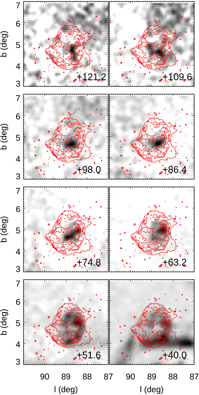
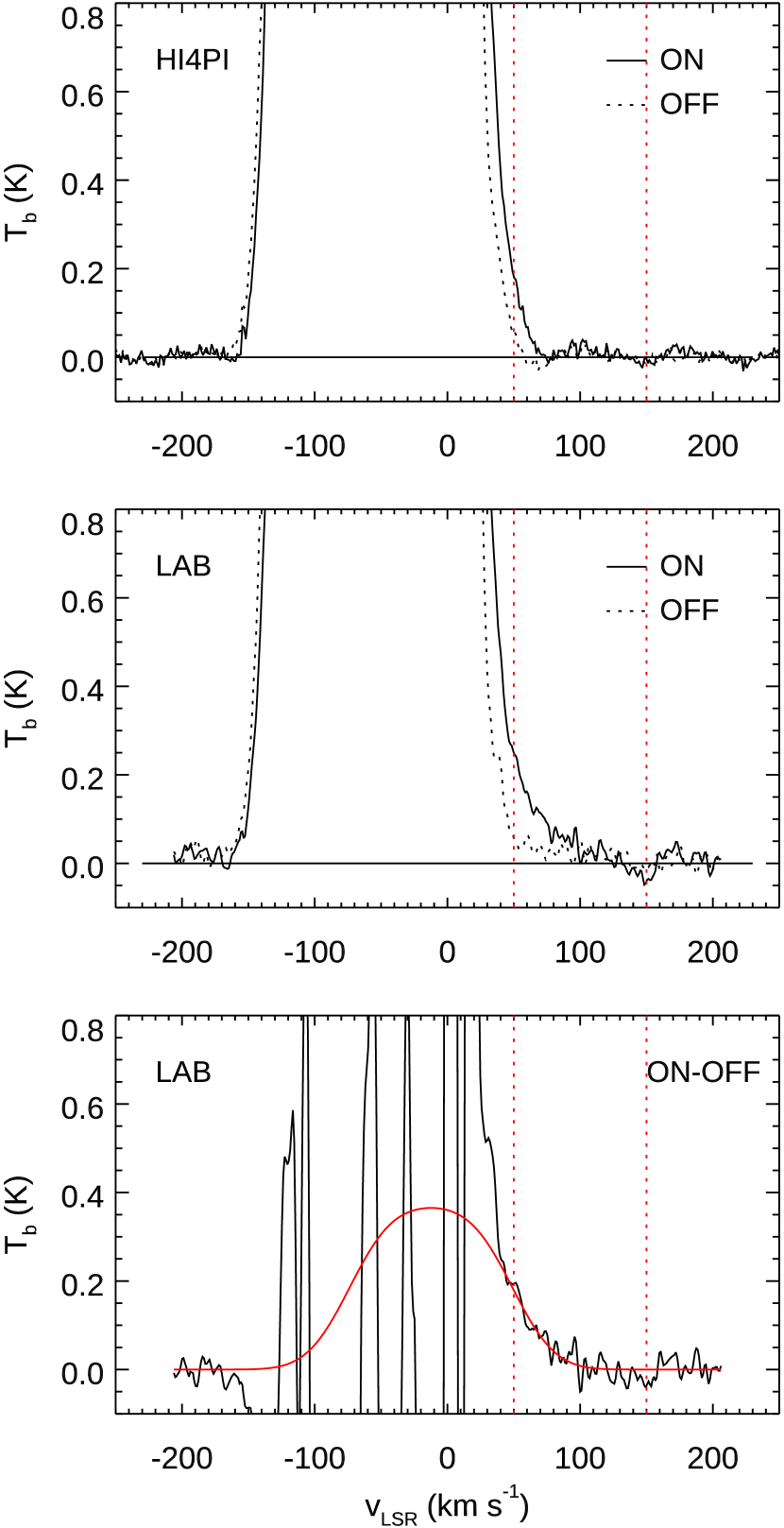
Figure 9: Left: Hi channel maps of the fast-expanding Hi shell in HB 21. Red contours show the SNR morphology in radio continuum obtained by the Dominion Radio Astrophysical Observatory (DRAO) (see Byun et al., 2006). Each map has been obtained by integrating over $11.6$ km s^-1 centered at the labeled $v_{\rm LSR}$ (km s^-1) and its gray scale is normalized by the maximum brightness. Top right: Source and background Hi 21 cm profiles of HB 21 from the HI4PI data. The source profile is the average profile inside the circular area of radius $1.\!\!^{\circ}1$ centered at $(l,b)=(88.\!\!^{\circ}92,4.\!\!^{\circ}75)$, while the background profile is the average profile inside the annulus of inner and outer radii of $1.\!\!^{\circ}4$ and $1.\!\!^{\circ}7$, respectively. Middle right: Same as the top right but from the LAB data. Bottom right: Background-subtracted Hi spectrum of HB 21 from the LAB data and a fit. Variations in Hi 21 cm brightnesses between the source and background directions cause the wild fluctuations in this background-subtracted profile at low velocities. The red solid line is a best fit to the profile between the velocity range marked by the red dotted lines (i.e., 50–150 km s^-1).

Appendix B Thermal Energy and Distance of G54.4$-0.3$

B.1 Thermal Energy

X-ray emission from SNR G54.4$-$0.3 has been detected with ROSAT, ASCA, and Chandra. G54.4$-$0.3 shows diffuse X-ray emission with a centrally-peaked morphology surrounded by a roughly circular radio shell with a radius of $R$ $\sim$ 20^′ (Figure 10a, Park et al. 2013). Taking advantage of the large field of view (50^′ in diameter) and the broad spectral coverage ($E$ $\sim$ 0.3 – 10 keV), we use the archival ASCA Gas Imaging Spectrometer (GIS) data to estimate the thermal energy of G54.4$-$0.3. Three ObsIDs in the ASCA pulic archive cover the entire G54.4$-$0.3 (Figure 10a). We extracted the source spectrum from a circular region with an angular radius $R$ = 12^′, centered on RA(J2000) = 19^h 33^m 10^s.92, Dec(J2000) = 19$\arcdeg$ 03^′ 15$.\mkern-4.0mu^{\prime\prime}$7 (the yellow circle in Figure 10a) in ObsID 52000000 (pointing at the central X-ray emission feature of G54.4$-$0.3, the middle cyan circle in Figure 10a). This region includes the bulk of the centrally-peaked X-ray emission in this SNR. The soft X-ray image from ROSAT data shows a pointlike emission feature near the center of the SNR (Figure 10a). This source is faint in the ASCA GIS data, whose fractional contribution in our source spectrum is negligible ($\sim$5% in the 0.5 – 9 keV band flux, assuming a source region with a radius of 2^′). Thus, we did not remove this source in our source spectral extraction. We extracted the background spectrum from a circular region just outside of the northern radio shell based on ObsID 52001000 (the white circle in Figure 10a). For our spectral extraction, we used the standard pipeline-processed event files in the ASCA public archive. We combined GIS2 and GIS3 data for both of the source and background spectra. The total effective exposures are $\sim$37 ks and $\sim$34 ks for the extracted source and background spectra, respectively. Based on these data, we collected $\sim$4300 background-subtracted source counts in the 0.6 – 8 keV band.

The extracted X-ray spectrum of G54.4$-$0.3 can be fitted with two-component spectral models for thermal or non-thermal origins. For the thermal component, we consider X-ray emission from the shocked optically-thin hot gas in either collisional ionization equilibrium (CIE, the APEC model in XSPEC [Arnaud 1996]), or non-equilibrium ionization (NEI, the “plane-shock” model, PSHOCK [Borkowski et al. 2001] in XSPEC). We fit the non-thermal component with a simple power law (PL) model. For our spectral model fits, we re-grouped the X-ray spectrum of G54.4$-$0.3 to achieve a minimum of 20 counts per photon energy channel. The observed X-ray spectrum of G54.4$-$0.3 can be fitted with either APEC + PSHOCK or APEC + PL models. In these spectral model fits, the soft thermal APEC component may be replaced with a PSHOCK component. In such a case, because the best-fit soft PSHOCK component model indicated large values of the ionization timescale of $\tau>10^{13}$ cm^-3 s ($\tau$ = $n_{e}t$, where $n_{e}$ is the postshock electron density and $t$ is the time since the gas has been shocked), which is equivalent with a CIE condition, we consider the APEC model for the soft component X-ray emission in the following discussion. Both of the best-fit APEC + PSHOCK and APEC + PL models are statistically acceptable with equally good fits ($\chi^{2}/\nu=206.1/194$ for APEC + PSHOCK, and $\chi^{2}/\nu=213.0/195$ for APEC + PL). We find that the best-fit elemental abundance is generally low ($\mathrel{\hbox{\hbox to0.0pt{\hbox{\lower 4.0pt\hbox{$\sim$}}\hss}\hbox{$<$}}}$1 solar with respect to the solar abundance by Anders & Grevesse (1989)). Thus, we fixed the abundance at the solar value in our spectral model fits, which is in line with the low-abundant interstellar origin for the observed X-ray emission in this old SNR. The best-fit parameters for our APEC + PSHOCK model fit are: the absorbing foreground H column $N({\rm H})_{\rm X-ray}=1.07^{+0.13}_{-0.16}\times 10^{22}$ cm^-2, the electron temperature $k_{B}T_{\rm APEC}=0.33^{+0.09}_{-0.06}$ keV, $k_{B}T_{\rm PSHOCK}=10.5^{+5.8}_{-3.0}$ keV, the ionization timescale $\tau=2.3^{+2.5}_{-2.1}\times 10^{9}$ cm^-3 s. Our best-fit APEC + PL model shows similar results for the soft APEC component ($k_{B}T_{\rm APEC}=0.38^{+0.12}_{-0.08}$ keV absorbed by $N({\rm H})_{\rm X-ray}=1.01\pm 0.15\times 10^{22}$ cm^-2). The best-fit PL component indicates the photon index $\Gamma=1.53^{+0.23}_{-0.26}$. In Figure 10b we show the ASCA GIS spectrum of G54.4$-$0.3 with the best-fit APEC+PSHOCK model overlaid.

The spectrally-soft component from the hot gas in CIE condition (fitted with $k_{B}T\sim 0.3$ keV) may be reasonable for X-ray emission from an old SNR. However, it is difficult to interpret the hard component emission with an extremely high electron temperature of $k_{B}T\sim 10$ keV with a very low $\tau$ as suggested by our APEC + PSHOCK model fit. The estimated electron temperature is similar to that of the Galactic ridge X-ray emission (GRXE), i.e., the diffuse X-ray emission from the thin disk surrounding the Galactic midplane (Warwick et al., 1985; Valinia & Marshall, 1998). So the GRXE may partially contribute to the hard component emission, although it is relatively weak at $\ell\sim 54^{\circ}$. This spectrally-hard component of the X-ray emission is equally fitted with a PL model with $\Gamma\sim 1.5$, which may also allow us alternative interpretations such as the shock-accelerated synchrotron emission from a separate young SNR projected along the LOS. In fact, G54.4$-$0.3 is projected against a complex of numerous radio shells, suggesting its location in a region with a strong star-forming activity. The origin and physical interpretations of the spectrally-hard component remain puzzling. Further studies based on deeper X-ray observations and hydrodynamic calculations may be required to reveal the true nature of the hard X-ray emission in the G54.4$-$0.3 region, which is beyond the scope of this work. For the purposes of this work, we conclude that the X-ray spectrum of G54.4$-$0.3 is most likely dominated by the soft thermal component.

Based on the best-fit volume emission measure of the soft APEC model component ($EM=\int n_{e}n_{\rm H}dV=$ (1.3–1.8)$\times 10^{58}$ cm^-5 where $n_{\rm H}$ is the H density), we estimate an average electron density $\bar{n}_{e}$. In this calculation we assumed $n_{e}\approx 1.2n_{\rm H}$ for a fully-ionized hot gas of cosmic abundance. We also assume a cylindrical volume for the derived volume emission measure with an angular radius $12^{\prime}$ and a path length (along the LOS) corresponding to the physical diameter of the spherical SNR ($2R=40^{\prime}$). We adopt 6.6 kpc as the distance to the SNR (see Appendix B.2). Our estimated average electron density is $\bar{n}_{e}\sim 0.07$ cm^-3. The mass of X-ray emitting gas inferred from the observed $EM$ is $M_{X}\approx 1.4m_{\rm H}\times EM/\bar{n}_{e}\sim 260$ $M_{\odot}$ where $m_{\rm H}$ is the mass of hydrogen nucleon. Assuming that the interior of the SNR is filled with hot gas in pressure equilibrium, we estimate the thermal energy of the SNR to be $E_{\rm th}\approx 3\bar{n}_{e}k_{B}TV_{s}\sim 8\times 10^{50}$ erg where $V_{s}$ is a spherical volume of radius $20^{\prime}$ (=38 pc at 6.6 kpc).

B.2 Distance

The distance to G54.4$-$0.3 is uncertain. There is a CO shell-like structure surrounding the SNR at $v_{\rm LSR}\sim 40$ km s^-1, and the distances between the near (3.3 kpc) and far (6.6 kpc) kinematic distances corresponding to this velocity have been proposed (Junkes et al., 1992a; Zychová & Ehlerová, 2016; Ranasinghe & Leahy, 2017). Another distance estimate can be obtained by comparing the X-ray absorbing column density $N({\rm H})_{\rm X-ray}(\sim 1\times 10^{22}$ cm^-2; Appendix B.1) to the Hi$+$H₂ column densities along the LOS to the SNR. In Figure 11, we show Hi 21 cm and ¹³CO $J$=1–0 emission line profiles toward G54.4$-$0.3 extracted from the VLA Galactic Plane Survey (Stil et al., 2006) and the Boston University-Five College Radio Astronomy Observatory Galactic Ring Survey (Jackson et al., 2006), respectively. The emission profiles are the average profiles of the X-ray emitting SNR area (i.e., the area bounded by the yellow circle in Fig. 10). In Figure 11, the emission at $v_{\rm LSR}>0$ km s^-1 is basically from the Hi gas inside the solar circle, so that if we add up all the emission at $v_{\rm LSR}>0$ km s^-1  it yields the total gas column density up to the opposite side of the solar circle at $\sim 10$ kpc in $\ell=54.\!\!^{\circ}4$. We derive $N({\rm HI})=0.92\times 10^{22}$ cm^-2 assuming Hi spin temperature of 150 K. For the H₂ column density, we derive $N({\rm H}_{2})\sim 4\times 10^{20}$ cm^-2 from the average integrated ¹³CO $J$=1–0 intensity of 1.3 K km s^-1 assuming that ¹³CO gas is in local thermodynamic equilibrium (LTE) with an excitation temperature of 10 K and $N({\rm H}_{2})/N({{}^{13}}{\rm CO})/=5\times 10^{5}$ (e.g., Dickman, 1978). This LTE ¹³CO column density may underestimate the true ¹³CO column density by a factor of 2–3 (Padoan et al., 2000; Szűcs et al., 2016), in which case the column density of H nuclei in molecular gas could be as much as $\sim 30$% of the atomic gas. Hence, the total H column density up to 10 kpc in $\ell=54.\!\!^{\circ}4$ is estimated to be about $1.2\times 10^{22}$ cm^-2, and, if we naively assume that about half of this column resides on the near side of the tangent point, the foreground X-ray absorbing column density $N({\rm H})_{\rm X-ray}\sim 1\times 10^{22}$ cm^-2 implies that the SNR G54.4$-$0.3 is probably beyond the tangential point. This is consistent with the conclusion of Ranasinghe & Leahy (2017) based on their Hi 21 cm absorption line study. So we adopt the far kinematic distance of the CO shell (6.6 kpc), as the distance of G54.4$-$0.3.

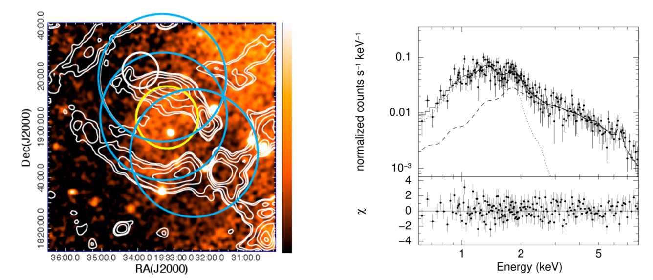
Figure 10: Left: A smoothed false-color ROSAT PSPC image of G54.4$-$0.3. The image has been taken from NASA’s SkyView on-line facility. The radio contours (taken from the Green Bank 4850 MHz survey) are overlaid. Cyan circles show the field of views of three archival ASCA GIS ObsIDs that detected G54.4$-$0.3. Our source and background regions for G54.4$-$0.3 are marked with a yellow and a white circle, respectively. Right: The ASCA GIS spectrum of G54.4$-$0.3. The best-fit APEC (dotted) + PSHOCK (dashed) model is overlaid. The bottom panel is residuals from the best-fit model.

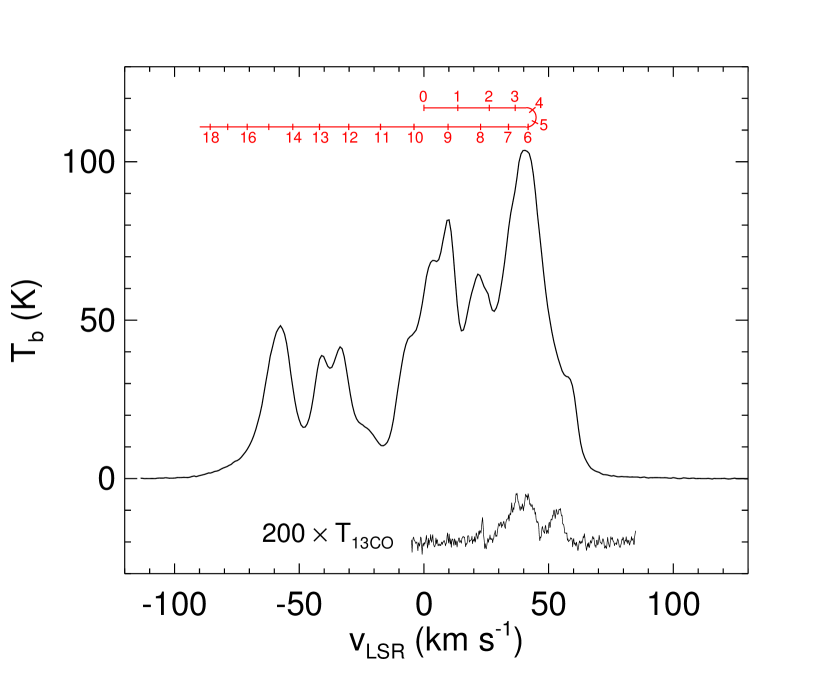
Figure 11: Average Hi 21 cm and ¹³CO $J$=1–0 emission line profiles toward G54.4$-$0.3. The ruler on top of the profile shows how the heliocentric distance varies as a function of LSR velocity. We have adopted the Galactic rotation curve of Reid et al. (2014) where the Galactocentric radius of the Sun $R_{0}=8.34$ kpc and the Galactic rotation speed at the solar circle $\Theta_{0}=220$ km s^-1.

Appendix C Thermal Energy of CTB 80

CTB 80 is a peculiar SNR with a pulsar wind nebula (PWN) embedded in an extended structure of complex morphology in radio (Figure 12). There is a 39.5 ms pulsar with the spin-down age of $1.1\times 10^{5}$ yr at the center of the PWN, suggesting that CTB 80 is an old SNR (Kulkarni et al., 1988; Fruchter et al., 1988). This pulsar, PSR 1951+32, is located at the eastern inner boundary of a nearly complete spherical shell of $\sim 1\arcdeg$ diameter with prominent infrared (IR) dust emission (Fesen et al., 1988). The detection of fast-expanding Hi shell with a dynamical age of $\sim 8\times 10^{4}$ yr (at 2 kpc) matching the shape of the IR shell supports that the IR shell is the SNR shell of CTB 80 (Koo et al., 1990). X-ray emission associated with PSR 1951+32 and its nebula has been studied in detail, but the study on the thermal X-ray emission from the SNR is scarce. Safi-Harb et al. (1995) studied the X-ray emission of CTB 80 with the Position Sensitive Proportional Counter (PSPC) aboard ROSAT, and proposed that the soft X-ray emission in the southeastern area of the field is associated with the SNR (see Fig. 12). The X-ray emission, however, extends much further away beyond the SNR shell, and it is difficult to reconcile the spatial distribution of the X-ray emission with the spherical SNR shell. Mavromatakis et al. (2001) detected optical filaments overlapping with the X-ray emission outside the SNR shell and suggested that they do not appear to be related to CTB 80, while Leahy & Ranasinghe (2012) studied Hi emission surrounding CTB 80 and proposed that CTB 80 is a larger ($R\sim 76^{\prime}$) SNR including the X-ray emission beyond the IR SNR shell.

Figure 12 shows the ROSAT X-ray and the Green Bank 4.85 GHz maps of the $3\arcdeg\times 2.\!\!^{\circ}6$ area surrounding CTB 80. The cyan circle represents the location of the IR SNR shell of radius $32^{\prime}$. The diffuse X-ray emission features mentioned above are labeled by “A” and “B”; source A for the X-ray emission inside the IR shell and source B for that outside the IR shell. We also see a bright extended X-ray filament (hereafter source “C”). Yoshita et al. (2000) showed that the X-ray emission of source C is thermal ($T\sim 0.4$ keV) with ASCA and ROSAT. They noted that there is a large radio filament overlapping with source C and concluded that these radio and X-ray filaments are portions of an old SNR (see Fig. 12:Right). We note that the radio filament extends further out to west and overlaps with source B. Hence, it seems reasonable to consider that sources B and C and the associated radio filament are the structures belong to another evolved SNR and that only source A is associated with CTB 80. In the following, we derive the thermal energy of source A.

Based on the archival ROSAT PSPC data (ObsID RP400048A00, $\sim$5 ks exposure time), we extract the X-ray spectrum of CTB 80 from a $\sim$48^′ $\times$ 36^′ region (the “Src” region, excluding the pulsar/PWN, in Figure 13:Left) corresponding to the central area of source A. The background spectrum was extracted from “source-free” regions off-axis to west (dashed circles in Figure 13:Left). The X-ray spectrum of CTB 80 shows significant fluxes at $E$ $<$ 0.5 keV, for which a low foreground column ($N_{\rm H}$ $\sim$ 10²⁰ cm^-2) is implied due to the short mean free path for X-ray photons at these energies. We note that the foreground column for PSR 1951+32, which is presumed to be associated with CTB 80, was estimated to be $N_{\rm H}=3\times 10^{21}$ cm^-2 (Safi-Harb et al., 1995). Indeed we find that the ROSAT PSPC spectrum of PSR 1951+32 shows negligible fluxes at $E$ $<$ 0.5 keV. Assuming the same $N_{\rm H}$ = 3 $\times$ 10²¹ cm^-2 for CTB 80, we conclude that the observed X-ray flux at $E$ $<$ 0.5 keV should be the foreground emission unrelated to CTB 80. We therefore have limited our spectral analysis of CTB 80 at $E>0.5$ keV, where we obtain $\sim$4800 background-subtracted counts. We rebinned the spectrum to contain at least 20 counts per energy channel, and fitted it with the X-ray emission spectral model of hot plasma in collisional ionization equilibrium (APEC model in XSPEC). In our spectral model fits, we fixed the absorbing column at $N_{\rm H}=3\times 10^{21}$ cm^-2, and the abundances at solar (Anders & Grevesse, 1989). The spectrum can be fitted with a two-component APEC model ($\chi^{2}/{\nu}$ = 117.9/106). The best-fit electron temperatures are $kT_{\rm hard}=1.9^{+0.5}_{-0.3}$ keV and $kT_{\rm soft}=0.18{\pm}0.01$ keV. Their emission measures are $EM_{\rm hard}=4.8\times 10^{56}$ cm^-3 and $EM_{\rm soft}=3.0\times 10^{57}$ cm^-3, respectively. As in Appendix B.1, we estimate the average electron density $\bar{n}_{e}$ of the soft component assuming $n_{e}\approx 1.2n_{\rm H}$. We also assume that the derived volume emission measure is for a cylindrical volume with an angular radius $21^{\prime}(=\sqrt{48^{\prime}\times 36^{\prime}}/2)$ and a path length (along the LOS) corresponding to the physical diameter of the spherical SNR ($2R=64^{\prime}$), Our estimated average electron density is $\bar{n}_{e}\sim 0.08$ cm^-3. The mass of X-ray emitting gas inferred from the observed $EM$ is $M_{X}\approx 1.4m_{\rm H}\times EM/\bar{n}_{e}\sim 40$ $M_{\odot}$. Assuming that the interior of the SNR is filled with hot gas in pressure equilibrium, we estimate the thermal energy of the SNR to be $E_{\rm th}\approx 3\bar{n}_{e}k_{B}TV_{s}\sim 6\times 10^{49}$ erg where $V_{s}$ is a spherical volume of radius $32^{\prime}$ (=19 pc at 2 kpc).

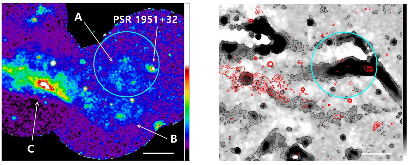
Figure 12: Left: A smoothed false-color ROSAT PSPC image of the $3\arcdeg\times 2.\!\!^{\circ}6$ area surrounding CTB 80. North is up and east is to the left. The image has been taken from NASA’s SkyView on-line facility. Cyan circle shows the boundary of the SNR defined by the IR shell (Fesen et al., 1988; Koo et al., 1990). The X-ray features discussed in the text are marked. Right: Radio 4.85 GHz image of the same area from the Green Bank 4850 MHz survey. The red contours shows the X-ray brightness distribution in the left image. In both images, the color (gray) scale is linear and the scale bar represents $0.\!\!^{\circ}5$.

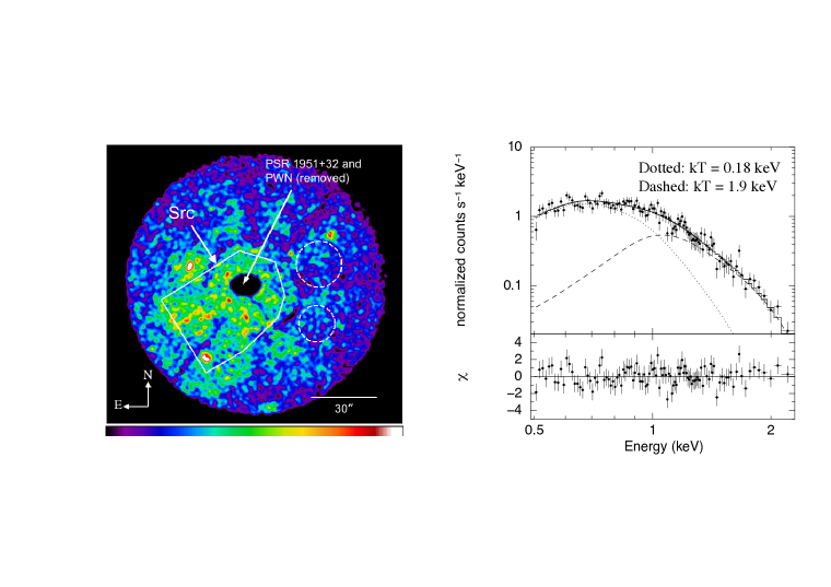
Figure 13: Left: A smoothed false-color ROSAT PSPC image of CTB 80. The areas used for the spectral analysis are marked. PSR 1951+32 and its associated PWN (Safi-Harb et al., 1995) has been removed. Right: The 0.5 – 2 keV band background-subtracted PSPC spectrum of CTB 80, as extracted from the Src region in the left image. The best-fit two-component APEC model is overlaid. The bottom panel is residuals from the best-fit model.

References

- Agertz et al. (2013) Agertz, O., Kravtsov, A. V., Leitner, S. N., & Gnedin, N. Y. 2013, ApJ, 770, 25
- Alarie & Drissen (2019) Alarie, A., & Drissen, L. 2019, MNRAS, 489, 3042
- Anders & Grevesse (1989) Anders, E., & Grevesse, N. 1989, Geochim. Cosmochim. Acta, 53, 197
- Arnal et al. (2000) Arnal, E. M., Bajaja, E., Larrarte, J. J., Morras, R., & Pöppel, W. G. L. 2000, A&AS, 142, 35
- Arnaud (1996) Arnaud, K. A. 1996, Astronomical Society of the Pacific Conference Series, Vol. 101, XSPEC: The First Ten Years, ed. G. H. Jacoby & J. Barnes, 17
- Asaoka & Aschenbach (1994) Asaoka, I., & Aschenbach, B. 1994, A&A, 284, 573
- Bajaja et al. (2005) Bajaja, E., Arnal, E. M., Larrarte, J. J., et al. 2005, A&A, 440, 767
- Bell (1978) Bell, A. R. 1978, MNRAS, 182, 147
- Bialy & Sternberg (2019) Bialy, S., & Sternberg, A. 2019, ApJ, 881, 160
- Blandford & Ostriker (1978) Blandford, R. D., & Ostriker, J. P. 1978, ApJ, 221, L29
- Blondin et al. (1998) Blondin, J. M., Wright, E. B., Borkowski, K. J., & Reynolds, S. P. 1998, ApJ, 500, 342
- Borkowski et al. (2001) Borkowski, K. J., Lyerly, W. J., & Reynolds, S. P. 2001, ApJ, 548, 820
- Braun & Strom (1986) Braun, R., & Strom, R. G. 1986, A&A, 164, 193
- Byun et al. (2006) Byun, D.-Y., Koo, B.-C., Tatematsu, K., & Sunada, K. 2006, ApJ, 637, 283
- Caprioli & Spitkovsky (2014) Caprioli, D., & Spitkovsky, A. 2014, ApJ, 783, 91
- Cazzolato & Pineault (2005) Cazzolato, F., & Pineault, S. 2005, AJ, 129, 2731
- Chevalier (1974) Chevalier, R. A. 1974, ApJ, 188, 501
- Chevalier & Li (1999) Chevalier, R. A., & Li, Z.-Y. 1999, ApJ, 520, L29
- Cho et al. (2015) Cho, W., Kim, J., & Koo, B.-C. 2015, Journal of Korean Astronomical Society, 48, 139
- Choi & Stone (2012) Choi, E., & Stone, J. M. 2012, ApJ, 747, 86
- Cioffi et al. (1988) Cioffi, D. F., McKee, C. F., & Bertschinger, E. 1988, ApJ, 334, 252
- Cowie & McKee (1977) Cowie, L. L., & McKee, C. F. 1977, ApJ, 211, 135
- Cowie et al. (1981) Cowie, L. L., McKee, C. F., & Ostriker, J. P. 1981, ApJ, 247, 908
- Cox (1972) Cox, D. P. 1972, ApJ, 178, 159
- Cox et al. (1999) Cox, D. P., Shelton, R. L., Maciejewski, W., et al. 1999, ApJ, 524, 179
- Dame et al. (2001) Dame, T. M., Hartmann, D., & Thaddeus, P. 2001, ApJ, 547, 792
- Dewangan et al. (2018) Dewangan, L. K., Baug, T., Ojha, D. K., Zinchenko, I., & Luna, A. 2018, ApJ, 864, 54
- Dickman (1978) Dickman, R. L. 1978, ApJS, 37, 407
- Dickman et al. (1992) Dickman, R. L., Snell, R. L., Ziurys, L. M., & Huang, Y.-L. 1992, ApJ, 400, 203
- Diesing & Caprioli (2018) Diesing, R., & Caprioli, D. 2018, Physical Review Letters, 121, 091101
- Draine (2011) Draine, B. T. 2011, Physics of the Interstellar and Intergalactic Medium (Princeton: Princeton University Press)
- Driessen et al. (2018) Driessen, L. N., Domček, V., Vink, J., et al. 2018, ApJ, 860, 133
- El-Badry et al. (2019) El-Badry, K., Ostriker, E. C., Kim, C.-G., Quataert, E., & Weisz, D. R. 2019, MNRAS, 490, 1961
- Fesen et al. (1988) Fesen, R. A., Shull, J. M., & Saken, J. M. 1988, Nature, 334, 229
- Field (1965) Field, G. B. 1965, ApJ, 142, 531
- Field et al. (1969) Field, G. B., Goldsmith, D. W., & Habing, H. J. 1969, ApJ, 155, L149
- Foster et al. (2013) Foster, J. B., Rathborne, J. M., Sanhueza, P., et al. 2013, PASA, 30, e038
- Fruchter et al. (1988) Fruchter, A. S., Taylor, J. H., Backer, D. C., Clifton, T. R., & Foster, R. S. 1988, Nature, 331, 53
- Gentry et al. (2019) Gentry, E. S., Krumholz, M. R., Madau, P., & Lupi, A. 2019, MNRAS, 483, 3647
- Gerbrandt et al. (2014) Gerbrandt, S., Foster, T. J., Kothes, R., Geisbüsch, J., & Tung, A. 2014, A&A, 566, A76
- Giacani et al. (1997) Giacani, E. B., Dubner, G. M., Kassim, N. E., et al. 1997, AJ, 113, 1379
- Giovanelli & Haynes (1979) Giovanelli, R., & Haynes, M. P. 1979, ApJ, 230, 404
- Gnat & Ferland (2012) Gnat, O., & Ferland, G. J. 2012, ApJS, 199, 20
- Green (2019) Green, D. A. 2019, Journal of Astrophysics and Astronomy, 40, 36
- Harrus et al. (1997) Harrus, I. M., Hughes, J. P., Singh, K. P., Koyama, K., & Asaoka, I. 1997, ApJ, 488, 781
- Hartmann & Burton (1997) Hartmann, D., & Burton, W. B. 1997, Atlas of Galactic Neutral Hydrogen (Cambridge: Cambridge University Press)
- HI4PI Collaboration et al. (2016) HI4PI Collaboration, Ben Bekhti, N., Flöer, L., et al. 2016, A&A, 594, A116
- Hopkins et al. (2014) Hopkins, P. F., Kereš, D., Oñorbe, J., et al. 2014, MNRAS, 445, 581
- Hopkins et al. (2018) Hopkins, P. F., Wetzel, A., Kereš, D., et al. 2018, MNRAS, 477, 1578
- Hu (2019) Hu, C.-Y. 2019, MNRAS, 483, 3363
- Hurley-Walker et al. (2019) Hurley-Walker, N., Gaensler, B. M., Leahy, D. A., et al. 2019, PASA, 36, e048
- Iffrig & Hennebelle (2015) Iffrig, O., & Hennebelle, P. 2015, A&A, 576, A95
- Inoue & Omukai (2015) Inoue, T., & Omukai, K. 2015, ApJ, 805, 73
- Jackson et al. (2006) Jackson, J. M., Rathborne, J. M., Shah, R. Y., et al. 2006, ApJS, 163, 145
- Jeong et al. (2013) Jeong, I.-G., Koo, B.-C., Cho, W.-K., et al. 2013, ApJ, 770, 105
- Junkes et al. (1992a) Junkes, N., Fuerst, E., & Reich, W. 1992a, A&AS, 96, 1
- Junkes et al. (1992b) —. 1992b, A&A, 261, 289
- Kalberla et al. (2005) Kalberla, P. M. W., Burton, W. B., Hartmann, D., et al. 2005, A&A, 440, 775
- Kang & Koo (2007) Kang, J.-h., & Koo, B.-C. 2007, ApJS, 173, 85
- Kang et al. (2012) Kang, J.-h., Koo, B.-C., & Salter, C. 2012, AJ, 143, 75
- Kang et al. (2014) Kang, P. K., Anna, P., Nunes, J. P., et al. 2014, Geophys. Res. Lett., 41, 6184
- Katz (1992) Katz, N. 1992, ApJ, 391, 502
- Kim et al. (2008) Kim, C.-G., Kim, W.-T., & Ostriker, E. C. 2008, ApJ, 681, 1148
- Kim & Ostriker (2015) Kim, C.-G., & Ostriker, E. C. 2015, ApJ, 802, 99
- Kim & Ostriker (2018) —. 2018, ApJ, 853, 173
- Kim et al. (2014) Kim, C.-G., Ostriker, E. C., & Kim, W.-T. 2014, ApJ, 786, 64
- Kimm & Cen (2014) Kimm, T., & Cen, R. 2014, ApJ, 788, 121
- Klein et al. (1994) Klein, R. I., McKee, C. F., & Colella, P. 1994, ApJ, 420, 213
- Koo & Heiles (1991) Koo, B.-C., & Heiles, C. 1991, ApJ, 382, 204
- Koo & Kang (2004) Koo, B.-C., & Kang, J.-h. 2004, MNRAS, 349, 983
- Koo et al. (2004) Koo, B.-C., Kang, J.-H., & McClure-Griffiths, N. M. 2004, Journal of Korean Astronomical Society, 37, 61
- Koo et al. (2006) Koo, B.-C., Kang, J.-h., & Salter, C. J. 2006, ApJ, 643, L49
- Koo et al. (1995a) Koo, B.-C., Kim, K.-T., & Seward, F. D. 1995a, ApJ, 447, 211
- Koo & Moon (1997) Koo, B.-C., & Moon, D.-S. 1997, ApJ, 475, 194
- Koo et al. (1990) Koo, B.-C., Reach, W. T., Heiles, C., Fesen, R. A., & Shull, J. M. 1990, ApJ, 364, 178
- Koo et al. (2001) Koo, B.-C., Rho, J., Reach, W. T., Jung, J., & Mangum, J. G. 2001, ApJ, 552, 175
- Koo et al. (1993) Koo, D. C., Gronwall, C., & Bruzual A., G. 1993, ApJ, 415, L21
- Koo et al. (1995b) Koo, D. C., Guzman, R., Faber, S. M., et al. 1995b, ApJ, 440, L49
- Koo et al. (2016) Koo, J.-R., Lee, J. W., Hong, K., Kim, S.-L., & Lee, C.-U. 2016, AJ, 151, 77
- Koo et al. (2014) Koo, J.-R., Lee, J. W., Lee, B.-C., et al. 2014, AJ, 147, 104
- Kothes et al. (2005) Kothes, R., Uyanıker, B., & Reid, R. I. 2005, A&A, 444, 871
- Krumholz et al. (2014) Krumholz, M. R., Bate, M. R., Arce, H. G., et al. 2014, in Protostars and Planets VI, ed. H. Beuther, R. S. Klessen, C. P. Dullemond, & T. Henning, 243
- Kulkarni et al. (1988) Kulkarni, S. R., Clifton, T. C., Backer, D. C., Foster, R. S., & Fruchter, A. S. 1988, Nature, 331, 50
- Lazendic & Slane (2006) Lazendic, J. S., & Slane, P. O. 2006, ApJ, 647, 350
- Leahy & Ranasinghe (2012) Leahy, D. A., & Ranasinghe, S. 2012, MNRAS, 423, 718
- Lee et al. (2012) Lee, K.-S., Ferguson, H. C., Wiklind, T., et al. 2012, ApJ, 752, 66
- Lee et al. (2015) Lee, S.-H., Patnaude, D. J., Raymond, J. C., et al. 2015, ApJ, 806, 71
- Lee et al. (2019) Lee, Y.-H., Koo, B.-C., Lee, J.-J., Burton, M. G., & Ryder, S. 2019, AJ, 157, 123
- Lee et al. (2008) Lee, Y. S., Beers, T. C., Sivarani, T., et al. 2008, AJ, 136, 2022
- Leitherer et al. (1999) Leitherer, C., Schaerer, D., Goldader, J. D., et al. 1999, ApJS, 123, 3
- Li et al. (2015) Li, M., Ostriker, J. P., Cen, R., Bryan, G. L., & Naab, T. 2015, ApJ, 814, 4
- Markwardt (2009) Markwardt, C. B. 2009, in Astronomical Society of the Pacific Conference Series, Vol. 411, Astronomical Data Analysis Software and Systems XVIII, ed. D. A. Bohlender, D. Durand, & P. Dowler, 251
- Martizzi et al. (2015) Martizzi, D., Faucher-Giguère, C.-A., & Quataert, E. 2015, MNRAS, 450, 504
- Mavromatakis et al. (2001) Mavromatakis, F., Ventura, J., Paleologou, E. V., & Papamastorakis, J. 2001, A&A, 371, 300
- McKee & Ostriker (2007) McKee, C. F., & Ostriker, E. C. 2007, ARA&A, 45, 565
- McKee & Ostriker (1977) McKee, C. F., & Ostriker, J. P. 1977, ApJ, 218, 148
- Okon et al. (2020) Okon, H., Tanaka, T., Uchida, H., et al. 2020, ApJ, 890, 62
- Padoan et al. (2000) Padoan, P., Juvela, M., Bally, J., & Nordlund, Å. 2000, ApJ, 529, 259
- Pannuti et al. (2010) Pannuti, T. G., Rho, J., Borkowski, K. J., & Cameron, P. B. 2010, AJ, 140, 1787
- Park et al. (2013) Park, G., Koo, B.-C., Gibson, S. J., et al. 2013, ApJ, 777, 14
- Park et al. (2015) Park, J., Caprioli, D., & Spitkovsky, A. 2015, Phys. Rev. Lett., 114, 085003
- Piontek & Ostriker (2004) Piontek, R. A., & Ostriker, E. C. 2004, ApJ, 601, 905
- Pittard (2019) Pittard, J. M. 2019, MNRAS, 488, 3376
- Ranasinghe & Leahy (2017) Ranasinghe, S., & Leahy, D. A. 2017, ApJ, 843, 119
- Reach et al. (2005) Reach, W. T., Megeath, S. T., Cohen, M., et al. 2005, PASP, 117, 978
- Reid et al. (2014) Reid, M. J., Menten, K. M., Brunthaler, A., et al. 2014, ApJ, 783, 130
- Rho & Petre (1998) Rho, J., & Petre, R. 1998, ApJ, 503, L167
- Rho et al. (1994) Rho, J., Petre, R., Schlegel, E. M., & Hester, J. J. 1994, ApJ, 430, 757
- Rosdahl et al. (2017) Rosdahl, J., Schaye, J., Dubois, Y., Kimm, T., & Teyssier, R. 2017, MNRAS, 466, 11
- Safi-Harb et al. (1995) Safi-Harb, S., Ogelman, H., & Finley, J. P. 1995, ApJ, 439, 722
- Sashida et al. (2013) Sashida, T., Oka, T., Tanaka, K., et al. 2013, ApJ, 774, 10
- Schneider & Robertson (2017) Schneider, E. E., & Robertson, B. E. 2017, ApJ, 834, 144
- Sedov (1959) Sedov, L. I. 1959, Similarity and Dimensional Methods in Mechanics (NewYork: Academic)
- Seon & Kim (2020) Seon, K.-I., & Kim, C.-G. 2020, arXiv e-prints, arXiv:2005.00238
- Shelton et al. (1999) Shelton, R. L., Cox, D. P., Maciejewski, W., et al. 1999, ApJ, 524, 192
- Slane et al. (2015) Slane, P., Bykov, A., Ellison, D. C., Dubner, G., & Castro, D. 2015, Space Sci. Rev., 188, 187
- Slane et al. (2002) Slane, P., Smith, R. K., Hughes, J. P., & Petre, R. 2002, ApJ, 564, 284
- Slavin et al. (2017) Slavin, J. D., Smith, R. K., Foster, A., et al. 2017, ApJ, 846, 77
- Smith et al. (2018) Smith, M. C., Sijacki, D., & Shen, S. 2018, MNRAS, 478, 302
- Snowden et al. (1997) Snowden, S. L., Egger, R., Freyberg, M. J., et al. 1997, ApJ, 485, 125
- Stil et al. (2006) Stil, J. M., Taylor, A. R., Dickey, J. M., et al. 2006, AJ, 132, 1158
- Stone et al. (2020) Stone, J. M., Tomida, K., White, C. J., & Felker, K. G. 2020, arXiv e-prints, arXiv:2005.06651
- Sutherland & Dopita (1993) Sutherland, R. S., & Dopita, M. A. 1993, ApJS, 88, 253
- Szűcs et al. (2016) Szűcs, L., Glover, S. C. O., & Klessen, R. S. 2016, MNRAS, 460, 82
- Taylor (1950) Taylor, G. 1950, Royal Society of London Proceedings Series A, 201, 159
- Tenorio-Tagle et al. (1985) Tenorio-Tagle, G., Bodenheimer, P., & Yorke, H. W. 1985, A&A, 145, 70
- Thornton et al. (1998) Thornton, K., Gaudlitz, M., Janka, H. T., & Steinmetz, M. 1998, ApJ, 500, 95
- Tian & Leahy (2013) Tian, W. W., & Leahy, D. A. 2013, ApJ, 769, L17
- Tilley et al. (2006) Tilley, D. A., Balsara, D. S., & Howk, J. C. 2006, MNRAS, 371, 1106
- Troja et al. (2006) Troja, E., Bocchino, F., & Reale, F. 2006, ApJ, 649, 258
- Uchiyama et al. (2010) Uchiyama, Y., Blandford, R. D., Funk, S., Tajima, H., & Tanaka, T. 2010, ApJ, 723, L122
- Valinia & Marshall (1998) Valinia, A., & Marshall, F. E. 1998, ApJ, 505, 134
- Velázquez et al. (2004) Velázquez, P. F., Martinell, J. J., Raga, A. r. C., & Giacani, E. B. 2004, ApJ, 601, 885
- Vink (2012) Vink, J. 2012, A&A Rev., 20, 49
- Walch & Naab (2015) Walch, S., & Naab, T. 2015, MNRAS, 451, 2757
- Warwick et al. (1985) Warwick, R. S., Turner, M. J. L., Watson, M. G., & Willingale, R. 1985, Nature, 317, 218
- White & Frenk (1991) White, S. D. M., & Frenk, C. S. 1991, ApJ, 379, 52
- Wolfire et al. (1995) Wolfire, M. G., McKee, C. F., Hollenbach, D., & Tielens, A. G. G. M. 1995, ApJ, 453, 673
- Yoshita et al. (2000) Yoshita, K., Miyata, E., & Tsunemi, H. 2000, PASJ, 52, 867
- Zhang & Chevalier (2019) Zhang, D., & Chevalier, R. A. 2019, MNRAS, 482, 1602
- Zhang et al. (2015) Zhang, G.-Y., Chen, Y., Su, Y., et al. 2015, ApJ, 799, 103
- Zhang et al. (2019) Zhang, G.-Y., Slavin, J. D., Foster, A., et al. 2019, ApJ, 875, 81
- Zychová & Ehlerová (2016) Zychová, L., & Ehlerová, S. 2016, A&A, 595, A49