Learning Causal Representations for Robust Domain Adaptation

Abstract

Domain adaptation solves the learning problem in a target domain by leveraging the knowledge in a relevant source domain. While remarkable advances have been made, almost all existing domain adaptation methods heavily require large amounts of unlabeled target domain data for learning domain invariant representations to achieve good generalizability on the target domain. In fact, in many real-world applications, target domain data may not always be available. In this paper, we study the cases where at the training phase the target domain data is unavailable and only well-labeled source domain data is available, called robust domain adaptation. To tackle this problem, under the assumption that causal relationships between features and the class variable are robust across domains, we propose a novel Causal AutoEncoder (CAE), which integrates deep autoencoder and causal structure learning into a unified model to learn causal representations only using data from a single source domain. Specifically, a deep autoencoder model is adopted to learn low-dimensional representations, and a causal structure learning model is designed to separate the low-dimensional representations into two groups: causal representations and task-irrelevant representations. Using three real-world datasets the extensive experiments have validated the effectiveness of CAE compared to eleven state-of-the-art methods.

1 Introduction

In traditional machine learning, a fundamental assumption is that training data (source domain) and testing data (target domain) are drawn from the same distribution. However, in many practical scenarios, such as image classification, news recommendation and sentiment analysis, this assumption is often violated  [1, 2, 3].

To tackle this problem, a variety of domain adaptation methods have been proposed [4, 5, 6, 7, 8]. Assuming a source domain and a relevant target domain which have the same feature space but different probability distributions, domain adaptation aims to learn a set of domain invariant features that can generalize well to the target domain. Existing domain adaptation methods can be roughly grouped into two categories based on the approach taken: correlation-based methods, such as CDAN [9] and ALDA [5], and causality-based methods, such as Infer [10] and Prop [11].

Correlation-based methods learn invariant representations based on the correlations between features and the class variable. In general, correlations may not capture the causal relationships between features and the class variable, but only their co-occurrences, and thus correlation-based invariant representations may not guarantee good generalizability on the target domain. For instance, in a picture of a dog, those representations of the background features such as grass and blue sky may have a strong correlation with the label (dog), but they may not be transferable across different target domains, e.g. pictures taken at different locations or weather conditions, as they are not the causal features of a dog image.

To mitigate this problem, learning invariant causal representations between source and target domains from data has attracted much attention recently [10, 11]. Causal relationships reflect the underlying data generating mechanism and thus are persistent across different settings or environments. For instance, considering the picture of a dog again, features such as eyes, ears and face shape are the fundamental elements for recognizing a dog and they would not change no matter where and when the picture was taken.

Although domain adaptation has been studied quite intensively in recent years, most existing domain adaptation methods rely on the unlabeled target domain data for learning domain invariant representations [1]. Indeed, the target domain data provide an additional source of information for learning invariant representations with better generalizability. However, in practice, often only a very limited amount of target domain data is available, either because the target domain is evolving (e.g. an online movie review system for which new movies are produced all the time), or it is impossible to collect all samples in the target domain (e.g. a computer vision system for which it is impossible to collect samples for all different contexts). Therefore classifiers trained on the representations learnt by the existing methods may generalize well to the very small portion of the known target domain data, but their performance may deteriorate soon after being deployed in real life.

To alleviate the problem mentioned above, zero-shot domain adaptation (ZSDA) has been studied [12, 13, 14], which deals with the situation where the task-relevant target domain data is unavailable but the task-irrelevant source and target domain data is available during the training phase. For instance, ZSDA methods learn a prediction model for the color digit images (task-relevant target domain), given the grayscale digit images (task-relevant source domain), the grayscale letter images (task-irrelevant source domain), and the color letter images (task-irrelevant target domain). Existing methods [13, 12, 14] depend on the task-irrelevant target domain data for learning domain invariant representations to bridge the gap between source and target domains. However, in real-world scenarios, on the one hand, collecting sufficient task-irrelevant target domain data is expensive and time-consuming. On the other hand, when the difference between the collected task-irrelevant target domain data and task-relevant target domain data is substantially large, matching the distributions between the task-irrelevant dual-domain pairs may not well alleviate the distribution discrepancy between task-relevant source domain data and task-relevant target domain data.

Then a question naturally arises: when the task-relevant target domain data is inadequate or unavailable and the task-irrelevant target domain data is unavailable, can we learn domain invariant feature representations with good generalizability only using data of the source domain?

In this paper, we formulate this question as the robust domain adaptation problem for cases where the target domain data (both task-relevant and task-irrelevant target domain data) is unavailable and only a well-labeled source domain is available in the training phase. The key challenge for robust domain adaptation is how to reduce the distribution discrepancy between the source and unknown target domains.

Recent studies reveal that causal features enable more reliable predictions in non-static environment where the distributions of training and testing data may be different but related [15, 16, 17]. Using causal features of the class variable to built a prediction model is a reasonable way to address the problem of robust domain adaptation, since even if the source and target domains are not obtained from the same data distribution, the causal relationships between features and the class variable are robust across domains. For instance, we want to build a predictive model for recognizing dogs using the images with dogs on grass. Based on the images with dogs on grass, a prediction model built using non-causal features such as grass may not achieve good performance on the image with a dog in snow. In contrast, if the causal features (such as eyes, ears and face shape) are selected as the predictive features, a predictive model built on the images with dogs on grass will be robust to correctly classify an image with a dog in snow. Recently, a number of Markov Blanket (MB) discovery algorithms have been proposed for causal feature selection [18, 16]. The MB of the class variable consists of the parents (direct causes), children (direct effects), and spouses (other parents of the class variable’s children). For more details of MB, we refer readers to Appendix of this paper and related literature, e.g. [16, 18, 19]. Due to the robustness of causal features [15, 17], we can learn MB of the class variable for robust domain adaptation. However, high-dimensional data often deteriorate the performance of MB learning, due to the fact that when dimension increases, MB learning becomes unreliable given a limited number of samples. Furthermore, noise contained in data will make existing MB learning algorithms achieve inaccurate results.

Motivated by the aforementioned issues, in this paper, under the assumption that causal relationships between features and the class variable are robust across domains, we propose a novel Causal AutoEncoder (CAE) for learning robust causal representations only using data from a single source domain. Specifically, CAE jointly optimizes deep autoencoder and causal structure learning models to learn causal representations from the source domain data. The deep autoencoder model is adopted to map the input data into a low-dimensional feature space to reduce the influence of noise contained in data, and the causal structure learning model is used to separate the low-dimensional representations learnt with the deep autoencoder into two groups: causal representations (MB feature representations) and task-irrelevant representations (non-MB feature representations). The main contributions of the paper are summarized as follows.

• We investigate the robust domain adaptation problem in which the task-relevant and task-irrelevant target domain data is unknown during the model training phase.

• For robust domain adaptation, we design a causal autoencoder, which integrates autoencoder and causal structure learning into a unified model to learn causal representations.

• We have conducted extensive experiments using three public domain adaptation datasets, and have compared CAE with eleven state-of-the-art algorithms, to demonstrate the effectiveness and superiority of CAE.

2 Related Work

Our work is in the area of domain adaptation and is also related to domain generalization and stable learning. This section reviews the related work in the three areas and briefly introduces causal feature selection.

Domain adaptation. Existing domain adaptation methods fall into two broad categories based on the approach taken: correlation-based and causality-based methods.

Correlation-based domain adaptation methods have received increasing attentions from researchers because of their impressive performance [20, 21]. Generally, these methods can be autoencoder-based or adversarial-learning based. One typical autoencoder-based method is DTFC, which disturbs different features with different corruption probabilities to extract complex feature representations [22]. Nevertheless, DTFC only depends on the single autoencoder model, which presents a problem when extracting multiple characteristics of data. To alleviate this problem, SERA [23] and SEAE [24] tack two types of autoencoders in series to capture different characteristics of data in both domains. One typical adversarial-learning method is CDAN [9], which trains deep networks in a conditional domain-adversarial paradigm. To improve the transferability of deep neural networks, TransNorm [25] is presented. ALDA [5] integrates domain-adversarial learning and self-training into a unified framework to learn discriminative feature representations for accomplishing cross-domain tasks.

ZSDA [13] and CoCoGAN [12] focus on tackling the zero-shot domain adaptation problem, where the target-domain data for the task of interest is unavailable but the task-irrelevant dual-domain pairs data is available. Both methods rely on the information from task-irrelevant dual-domain pairs to complete cross-domain tasks. Our method differs from ZSDA and CoCoGAN because we only use the data from a single source domain and need not leverage the information from task-irrelevant dual-domain pairs.

Recently, several causality-based methods have been designed for domain adaptation, such as Infer [10] and Prop [11]. Infer  [10] uses a graphical model as a compact way to encode the change property of the joint distribution and then treats domain adaptation as a problem of Bayesian inference on the graphical models. Prop  [11] captures the underlying data generating mechanism behind the data distributions to accomplish cross-domain tasks.

We argue that existing domain adaptation methods leverage the target domain information or the information from task-irrelevant dual-domain pairs, but our method only uses the information from a single source domain.

Domain generalization. Domain generalization focuses on leveraging the knowledge in multiple related domains to promote the learning task in unseen domains [26]. A variety of domain generalization approaches have been designed, such as MTAE [26], MMD-AAE [27] and MASF [28]. MTAE [26] uses multi-task autoencoder to learn invariant features that are robust cross domains. MMD-AAE [27] learns latent feature representation by jointly optimizing a multi-domain autoencoder regularized by a classifier, the maximum mean discrepancy distance and an discriminator in an adversarial training manner. MASF [28] preserves inter-class relationships by aligning a derived soft confusion matrix, and encourages domain-independence while separating sample features and class-specific cohesion by using a metric-learning component. Recently, some causality-based methods have been proposed for domain generalization  [29, 30]. We argue that existing domain generalization methods rely on multiple source domains to explore the invariance properties, whereas our method only uses the data of a single source domain.

Stable learning. Stable learning deals with the challenging situation where only a single training data is available and the testing data is unavailable during the training phase [31, 32]. Stable learning focuses on tackling the problem of selection bias and model misspecification bias. Recently, several approaches have been designed for tackling sample selection bias problem, such as CRLR [33] and DGBR [31]. CRLR and DGBR balance the distribution of treated and control group by global sample weighting to isolate the clear effect of each predictor from the confounding variables. Despite their better performance, learning the weight for each sample is difficult in big data scenarios with huge training samples. To alleviate this issue, CVS [17] separates the causal variables by leveraging a seed variable. To deal with the problem of sample selection bias and model misspecification bias simultaneously, Shen et al. [32] reduce collinearity among input variables by sample reweighting, and Kuang et al. [34] force all features to be as independent as possible by jointly optimizing a weighted regression model and a variable decorrelation regularizer. These methods either reweight each sample or select causal features for stable learning, whereas our method learns causal representations for domain adaptation by jointly optimizing deep autoencoder and causal structure learning models.

Causal feature selection. Feature selection plays an essential role in high-dimensional learning tasks and it has been widely used in various practical scenarios. Traditional correlation-based feature selection methods exploit statistical associations or dependences between features and the class variable to make predictions, such as FCBF [35] and mRMR [36]. Correlation-based feature selection methods may capture spurious correlation, leading to unstable prediction across different environments. Recently, causal feature selection has attracted much attention from researchers [16], as it not only can improve the explanatory capability of predictive models but also can improve the robustness of predictive models. Learning Markov blanket (MB) for causal feature selection has been extensively studied in recent years, since the MB of the class variable is the optimal feature subset for feature selection [37]. Existing MB discovery methods can be roughly grouped into constraint-based methods and score-based methods. The former learns the MB of the class variable using conditional independence tests, such as HITON-MB [38] and BAMB [18], while the latter employs Bayesian score functions to discover MB instead of using conditional independence tests, such as SLL [39] and S²TMB [19]. Constraint-based MB discovery algorithms cannot distinguish direct causes of a target variable from its direct effects. Score-based algorithms can distinguish parents from children of a given variable, but they may suffer high computational complexity. For more details of MB, please refer to the Appendix.

3 The Proposed Causal AutoEncoder

In this section, we first formulate the robust domain adaptation problem to be tackled in this paper, and then introduce the proposed CAE algorithm in detail.

3.1 Problem Formulation

Robust Domain Adaptation. Given a labeled source domain $\mathcal{D}_{s}=[\textbf{X}_{s},\textbf{y}_{s}]$, where $\textbf{X}_{s}\in\mathbb{R}^{n\times d}$ and $\textbf{y}_{s}=(y_{1},...,y_{n})^{T}\in\mathbb{R}^{n\times 1}$ represent the source domain data of the features and class label $Y$, respectively. $n$ denotes the number of samples and $d$ denotes the dimension of feature space, $y_{i}$ is the label of the $i^{th}$ sample. Robust domain adaptation aims to leverage the knowledge in only one single source domain to learn a robust predication model for predicting the label of target domain data $\mathcal{D}_{t}=\textbf{X}_{t}$.

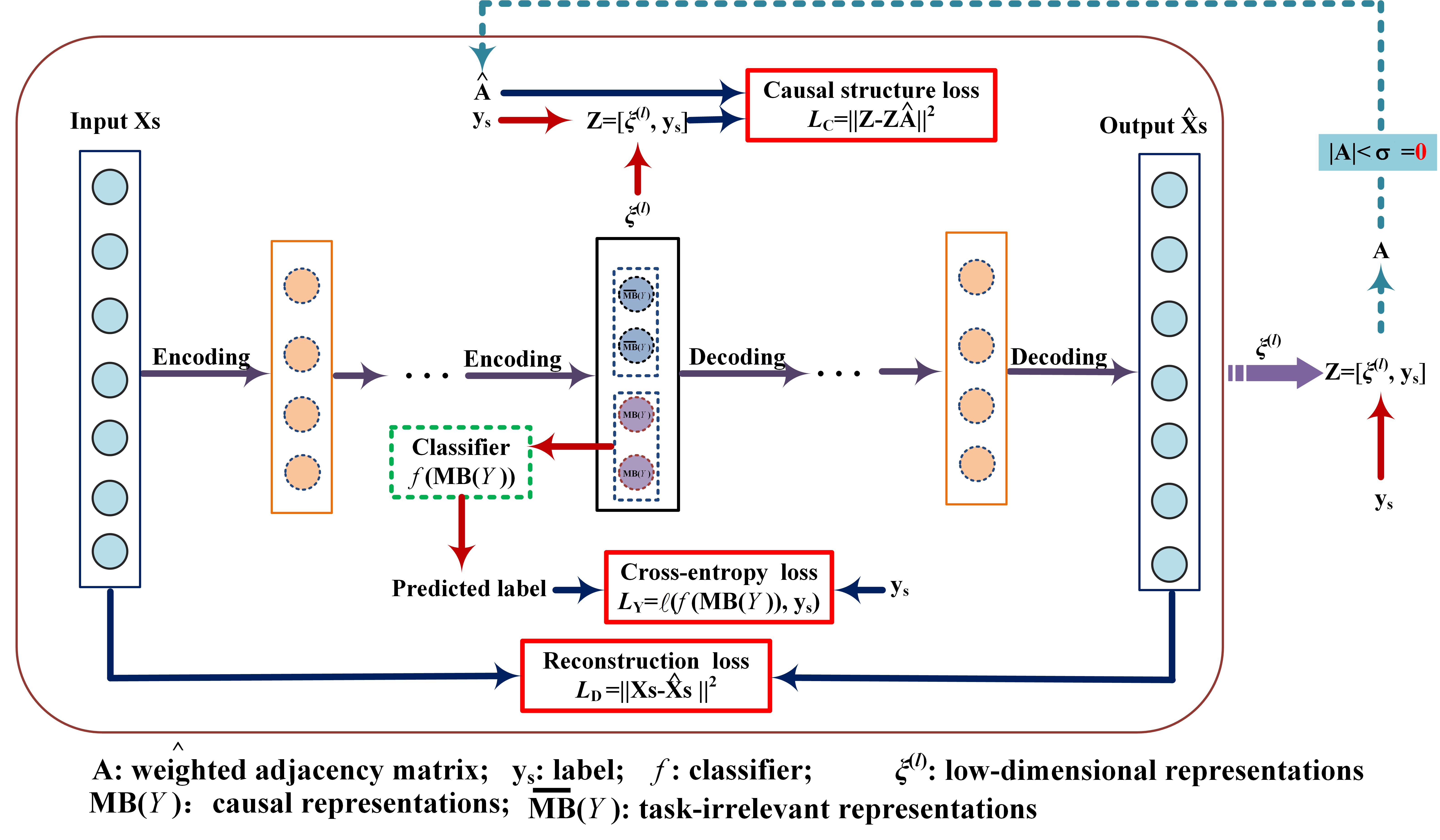
Figure 1: The framework of CAE.

3.2 Overview of CAE

We propose the Causal AutoEncoder (CAE) algorithm to learn causal representations for robust domain adaptation. The framework of CAE is illustrated in Fig.1. CAE has an input layer, an output layer and multiple hidden layers. Different from the traditional autoencoder, CAE incorporates the causal structure learning loss $\mathcal{L}_{C}$ and cross-entropy loss $\mathcal{L}_{Y}$ to learn robust causal low-dimensional representations with high generalizability for unknown target domain. The objective function to be minimized in CAE can be summarized as follows.

$$\mathcal{L}=\mathcal{L}_{D}+\lambda_{1}\mathcal{L}_{C}+\lambda_{2}\mathcal{L}_{Y}+\lambda_{3}\mathcal{L}_{R}.$$ (1)

where $\lambda_{1}$, $\lambda_{2}$ and $\lambda_{3}$ are the balancing parameters.

CAE learns low-dimensional representations by minimizing the construction error $\mathcal{L}_{D}$ between the input data $\textbf{X}_{s}$ and output data $\hat{\textbf{X}}_{s}$. To learn causal representations, CAE uses causal structure learning loss $\mathcal{L}_{C}$ to force the low-dimensional representations into two different groups, i.e. causal representations $\textbf{MB}(Y)$ and task-irrelevant representations $\overline{\textbf{MB}}$$(Y)$, as shown in Fig.1. The cross-entropy loss $\mathcal{L}_{Y}$ is used to optimize causal feature representations by incorporating the label information of source domain data. $\mathcal{L}_{R}$ is a regularization term on model parameters. In the following, we will give the details of CAE.

3.3 Reconstruction loss $\mathcal{L}_{D}$ and regularization loss $\mathcal{L}_{R}$

Recent studies reveal that even if the source and target domains are not obtained from the same data distribution, the causal relationships between features and the class variable are robust across relevant domains under different environments or settings [17, 31, 33]. Based on this, learning causal features of the class variable is a reasonable way to address the problem of robust domain adaptation. However, high-dimensional data often deteriorate the performance of causal feature learning. On the one hand, causal feature learning becomes unreliable on high-dimensional data given a limited number of samples. On the other hand, noise contained in data can lead to inaccurate results of existing causal feature learning algorithms. To alleviate these problems, CAE adopts a deep autoencoder model to map the input data into a low-dimensional feature space with high-level representations. CAE consists of two stages: encoding and decoding. Given input data $\textbf{X}_{s}$, CAE first encodes the input data to learn the low-dimensional feature representations through multiple nonlinear encoding processes, then decodes the low-dimensional representations to obtain the estimated output data $\hat{\textbf{X}}_{s}$. The process can be formalized as follows.

$${\rm Encoding:}\;\boldsymbol{\xi}^{(j)}=\sigma(\boldsymbol{\xi}^{(j-1)}\textbf{W}_{1}^{(j)}+\textbf{b}_{1}^{(j)}),j=1,2,\cdots,l.$$ (2)

$${\rm Decoding:}\;\boldsymbol{\psi}^{(j)}=\sigma(\boldsymbol{\psi}^{(j-1)}\textbf{W}_{2}^{(j)}+\textbf{b}_{2}^{(j)}),j=1,2,\cdots,l.$$

where $l$ is the number of hidden layers in the autoencoder and $\sigma$ is a nonlinear activation function (e.g., sigmoid function). Note that $\boldsymbol{\xi}^{(1)}$ = $\textbf{X}_{s}$ and $\boldsymbol{\psi}^{(1)}$ = $\boldsymbol{\xi}^{(l)}$, and $\boldsymbol{\xi}^{(l)}\in\mathbb{R}^{n\times k}$ ($k<d$ ) is the low-dimensional representations for $\textbf{X}_{s}$. $\textbf{W}_{1}^{(j)}$ and $\textbf{b}_{1}^{(j)}$ are the weight matrix and the bias vector on the $j^{th}$ encoding layer, respectively. For the $j^{th}$ decoding layer, $\textbf{W}_{2}^{(j)}$ and $\textbf{b}_{2}^{(j)}$ are its weight matrix and bias vector, respectively. The reconstruction error $\mathcal{L}_{D}$ (see Eq.(1)) between the input data $\textbf{X}_{s}$ and output data $\hat{\textbf{X}}_{s}$ = $\boldsymbol{\psi}^{(l)}$ in Eq.(1) is defined as follows.

$$\mathcal{L}_{D}=\frac{1}{2n}\|\textbf{X}_{s}-\hat{\textbf{X}}_{s}\|^{2}.$$ (3)

The last term in Eq.(1), i.e. $\mathcal{L}_{R}$, is a regularization term on model parameters, which is calculated as follows.

$$\mathcal{L}_{R}=\sum_{j=1}^{l}(||\textbf{W}_{1}^{(j)}||^{2}+||\textbf{b}_{1}^{(j)}||^{2}+||\textbf{W}_{2}^{(j)}||^{2}+||\textbf{b}_{2}^{(j)}||^{2}).$$ (4)

3.4 Causal structure learning loss $\mathcal{L}_{C}$

In order to reconstruct the input data $\textbf{X}_{s}$, the intrinsic information of input data needs to be captured by the low-dimensional feature representations $\boldsymbol{\xi}^{(l)}$. Therefore, $\boldsymbol{\xi}^{(l)}$ may contain some task-irrelevant information that cannot be used for cross-domain tasks, such as the background information in an image. Thus we hope to separate the low-dimensional representations into two groups: causal representations and task-irrelevant representations. Studies [16, 40] reveal that the Markov blanket (MB) of the class variable is the minimal feature subset with maximum predictivity for classification. Under the faithfulness assumption [41], all other features that are not in the MB set of the class variable are conditionally independent of the class variable conditioning on the MB set of the class variable. This means that the information of the non-MB feature representations are blocked given the MB feature representations. Motivated by this, in this paper, we treat the MB feature representations of the class variable as causal representations and other feature (non-MB features) representations as task-irrelevant representations, since the information of task-irrelevant representations are blocked by the MB feature representations. Thus, we need to identify MB feature representations of the class variable.

To achieve this goal, based on the learnt low-dimensional representations $\boldsymbol{\xi}^{(l)}$ and label information $\textbf{y}_{s}$ of source domain, we aim to learn a directed acyclic graph (DAG) $\mathbb{G}$ over Z, where $\textbf{Z}=[\boldsymbol{\xi}^{(l)},\textbf{y}_{s}]\in\mathbb{R}^{n\times(k+1)}$. In $\mathbb{G}$, $Z_{i}\in\textbf{Z}$ is a parent (i.e. a direct cause) of $Z_{j}$ and $Z_{j}$ is a child (i.e. a direct effect) of $Z_{i}$ if there is a directed edge from variable $Z_{i}$ to variable $Z_{j}$. Once $\mathbb{G}$ is obtained, we can identify the MB features of the class variable.

In the following, we give the details of learning a DAG $\mathbb{G}$ over Z. In this paper, we assume the same data generating procedure as in [42], i.e. the values of a variable is generated based on its direct causes, that is,

$$\footnotesize Z_{i}=g(Z_{pa(i)})+N_{i},i=1,2,\cdots,k+1.$$ (5)

where $Z_{pa(i)}$ represents the set of parent variables of variable $Z_{i}$, $g$ is a mapping function and $N_{i}$ is an additive noise.

Inspired by Zheng et al. [42], we encode the DAG $\mathbb{G}$ with the set of variables Z (i.e. the $k$-dimensional high-level feature representations and the class variable $\textbf{y}_{s}$) using an adjacency matrix A = $[\textbf{a}_{1}|\cdots|\textbf{a}_{k+1}]\in\mathbb{R}^{(k+1)\times(k+1)}$, where each column $\textbf{a}_{i}$ denotes the coefficients in the linear structural equation model of the form $Z_{i}$ = $\textbf{a}_{i}^{T}\textbf{Z}+N_{i}$ , or Z = ZA + N, where ZA is the estimated value for Z based on Z’s parents and we want the estimation as accurate as possible. To ensure the acyclicity of A, a constraint on A is adopted, as indicated in Theorem 1 below.

Theorem 1.

Let A $\in\mathbb{R}^{(k+1)\times(k+1)}$ be the (possibly negatively) weighted adjacency matrix of a directed graph, the graph is acyclic if and only if

$$\footnotesize tr\big{[}\big{(}\textbf{I}+\frac{\textbf{A}\odot\textbf{A}}{1+k}\big{)}^{(k+1)}\big{]}-(k+1)=0.$$

where $\odot$ is the Hadamard product, I is the the unit matrix.

Proof.

Let B = A $\odot$ A. Note that B is nonnegative. The binomial expansion reads

$$\footnotesize\big{(}\textbf{I}+\frac{\textbf{B}}{1+k}\big{)}^{(k+1)}=\textbf{I}+\sum_{j=1}^{k+1}\binom{k+1}{j}(\frac{1}{1+k})^{j}\textbf{B}^{j}.$$

It is known that there is a cycle of length $j$ if and only if $tr(\textbf{B}^{j})>0$ when B $\geq$ 0. Because if there is a cycle then there is a cycle of length at most $k+1$, we conclude that there is no cycle if and only if $tr\big{[}\big{(}\textbf{I}+\frac{\textbf{A}\odot\textbf{A}}{1+k}\big{)}^{(k+1)}\big{]}=tr(\textbf{I})=(k+1)=0$. ∎

To learn the $\mathbb{G}$ over $\textbf{Z}=[\boldsymbol{\xi}^{(l)},\textbf{y}_{s}]$, we integrate the above acyclicity constraint and the least-square loss between Z and ZA into one model as follows.

$$\ \quad\quad\quad\quad\quad\quad\min\limits_{\textbf{A}}\|\textbf{Z}-\textbf{Z}\textbf{A}\|^{2}$$ (6)

$${\rm subject}\quad{\rm to}\quad tr\big{[}\big{(}\textbf{I}+\frac{\textbf{A}\odot\textbf{A}}{1+k}\big{)}^{(k+1)}\big{]}-(k+1)=0.$$

We can first learn the low-dimensional feature representations $\boldsymbol{\xi}^{(l)}$. Based on the learnt $\boldsymbol{\xi}^{(l)}$, we obtain A by solving the optimization problem given in Eq.(6) following the process in reference [42]. That is, after obtaining a stationary point A of (6), given a fixed threshold $\sigma>$ 0, set any weights smaller than $\sigma$ in absolute value to zero. We obtain a new matric $\hat{\textbf{A}}$ by thresholding the edge weights of A as follows.

$$\hat{\textbf{A}}[i][j]=\left\{\begin{array}[]{lcl}{0},&if\quad|\textbf{A}[i][j]|<\sigma,\\ {\textbf{A}[i][j]},&otherwise.\end{array}\right.$$ (7)

There exists a directed edge from variable $Z_{i}$ to variable $Z_{j}$ if $|\textbf{A}[i][j]|\geq\sigma$.

Once $\hat{\textbf{A}}$ is learnt, we can identify the MB feature representations of class label through matrix $\hat{\textbf{A}}$, and we can separate the low-dimensional representations $\boldsymbol{\xi}^{(l)}$ into two groups: cause representations of the class variable $Y$, denoted as $\textbf{MB}(Y)$; and the other feature representations which are task-irrelevant (i.e. non-MB of $Y$), denoted as $\overline{\textbf{MB}}$$(Y)$, where $\boldsymbol{\xi}^{(l)}=\textbf{MB}(Y)\cup\overline{\textbf{MB}}(Y)$, and $\textbf{MB}(Y)\cap\overline{\textbf{MB}}(Y)=\emptyset$.

Since the causal relationships between the class variable and its MB features are robust across different settings or environments, we can use $\textbf{MB}(Y)$ as the causal features to build the prediction model to be used for the target domain. This requires that the low-dimensional feature representations learnt by CAE need to be consistent with the underlying causal mechanism or relations represented by $\hat{\textbf{A}}$. However, there is a difference between $\hat{\textbf{A}}$ and A, since the edge weights of A that are smaller than $\sigma$ in absolute value are set to zero. Hence, in learning low-dimensional feature representations, we use the learnt adjacency matrix $\hat{\textbf{A}}$ to constraint the low-dimensional representations as follows.

$$\quad\quad\mathcal{L}_{C}=\|\textbf{Z}-\textbf{Z}\hat{\textbf{A}}\|^{2}.$$ (8)

3.5 Cross-entropy loss $\mathcal{L}_{Y}$

To improve the quality of predictions using the causal feature representations, we incorporate the following cross-entropy loss into the objective function of CAE.

$$\mathcal{L}_{Y}=\ell(f(\textbf{MB}(Y)),\textbf{y}_{s}).$$ (9)

where $\ell$($\cdot$) is a cross-entropy loss, $f$ is a classifier which uses the causal feature representations. In this way, in the learning of the causal feature representations, CAE makes use of the label information of the samples in the source domain and aims to minimize prediction error of a classifier using the causal feature representations.

3.6 Optimization

Based on Eq.(3), Eq.(4), Eq.(8) and Eq.(9), the objective function of CAE in Eq.(1) can be written as:

$$\mathcal{L}= \frac{1}{2n}\|\textbf{X}_{s}-\hat{\textbf{X}}_{s}\|^{2}+\lambda_{1}\|\textbf{Z}-\textbf{Z}\hat{\textbf{A}}\|^{2}+\lambda_{2}\ell(f(\textbf{MB}(Y)),\textbf{y}_{s})$$ (10)

$$+\lambda_{3}\sum_{j=1}^{l}(||\textbf{W}_{1}^{(j)}||^{2}+||\textbf{b}_{1}^{(j)}||^{2}+||\textbf{W}_{2}^{(j)}||^{2}+||\textbf{b}_{2}^{(j)}||^{2}).$$

Now we show how to optimize the objective function. Note that the objective function involves several parameters, $\textbf{W}_{1}^{(j)},\textbf{b}_{1}^{(j)}$, $\textbf{W}_{2}^{(j)},\textbf{b}_{2}^{(j)}$ ($j=1,2,\cdots,l$) and $\hat{\textbf{A}}$. These parameters are dependent on each other, thus the problem cannot be solved directly. So we propose to update $\textbf{W}_{1}^{(j)},\textbf{b}_{1}^{(j)}$, $\textbf{W}_{2}^{(j)},\textbf{b}_{2}^{(j)}$ ($j=1,2,\cdots,l$) and $\hat{\textbf{A}}$ in an alternate manner. First, we initialize $\hat{\textbf{A}}$ as the unit matrix, and update $\textbf{W}_{1}^{(j)},\textbf{b}_{1}^{(j)}$, $\textbf{W}_{2}^{(j)},\textbf{b}_{2}^{(j)}$. Since we implement CAE using Tensorflow, once $\hat{\textbf{A}}$ is obtained, we use the Tensorflow framework to learn $\textbf{W}_{1}^{(j)},\textbf{b}_{1}^{(j)}$, $\textbf{W}_{2}^{(j)},\textbf{b}_{2}^{(j)}$ by minimizing the objective function in Eq.(10). Then, we fix $\textbf{W}_{1}^{(j)},\textbf{b}_{1}^{(j)}$, $\textbf{W}_{2}^{(j)},\textbf{b}_{2}^{(j)}$ and update $\hat{\textbf{A}}$.

We learn $\hat{\textbf{A}}$ by solving the problem in Eq.(6). Once A is learnt, we can obtain $\hat{\textbf{A}}$. We adopt the augmented Lagrangian method to solve the optimization problem given in Eq.(6). That is, from Eq.(6), we get the following augmented Lagrangian.

$$\mathcal{L}(\textbf{Z},\alpha,\rho)=\|\textbf{Z}-\textbf{Z}\textbf{A}\|^{2}+\alpha h(\textbf{A})+\frac{\rho}{2}|h(\textbf{A})|^{2}.$$ (11)

where $h(\textbf{A})=tr\big{[}\big{(}\textbf{I}+\frac{\textbf{A}\odot\textbf{A}}{1+k}\big{)}^{(k+1)}\big{]}-(k+1)$, $\alpha$ is the Lagrange multiplier, $\rho$ is is the penalty parameter. We update $\textbf{A},\alpha,\rho$ by using the following rules.

$$\textbf{A}^{(t+1)}=argmin\mathcal{L}(\textbf{Z},\alpha^{(t)},\rho^{(t)}),$$ (12)

$$\rho^{(t+1)}=\left\{\begin{array}[]{lcl}{10\rho^{(t)}},&if\quad|h(\textbf{A}^{(t+1)})|\geq\frac{1}{4}|h(\textbf{A}^{(t)})|,\\ {\rho^{(t)}},&otherwise.\end{array}\right.$$

$$\alpha^{(t+1)}=\alpha^{(t)}+\rho^{(t)}h(\textbf{A}^{(t+1)}).$$

where $t$ represents the $t^{th}$ iteration, $\rho^{(1)}$ = 1 and $\alpha^{(1)}=0$ are the initial values of $\rho$ and $\alpha$.

10:  Source domain data $\mathcal{D}_{s}=[\textbf{X}_{s},\textbf{y}_{s}]$ 2     Parameters $l$, $k$, $\lambda_{1}$, $\lambda_{2}$, $\lambda_{3}$ 30:  A, $\textbf{W}_{1}^{(j)},\textbf{b}_{1}^{(j)}$, $\textbf{W}_{2}^{(j)},\textbf{b}_{2}^{(j)}$, $j=1,2,\cdots,l$ 41:  Initialize parameters $\textbf{W}_{1}^{(j)},\textbf{b}_{1}^{(j)}$, $\textbf{W}_{2}^{(j)},\textbf{b}_{2}^{(j)}$ 52:  Initialize $\hat{\textbf{A}}$: ($k$+1)*I identity matrix 3:  Initialize the iteration variable $t\leftarrow 0$ 64:  Repeat 75:   $t\leftarrow t+1$; 86:   Fix $\hat{\textbf{A}}$, and update $\textbf{W}_{1}^{(j)},\textbf{b}_{1}^{(j)}$, $\textbf{W}_{2}^{(j)},\textbf{b}_{2}^{(j)}$ by Eq.(10); 97:   Fix $\textbf{W}_{1}^{(j)},\textbf{b}_{1}^{(j)}$, $\textbf{W}_{2}^{(j)},\textbf{b}_{2}^{(j)}$, and update A by Eq.(12); 108:   Obtain $\hat{\textbf{A}}$ by Eq.(7); 119:  Until $\mathcal{L}$ converges or max iteration is reached.

Algorithm 1 The Causal AutoEncoder (CAE).

The proposed CAE algorithm is summarized in Algorithm 1. The default value of the maximum iteration is set to 10, and the default value used for determining convergence is set to 1E-8 in Algorithm 1.

4 Experiments

In this section, we evaluate the effectiveness of CAE by comparing it with several feature selection and state-of-the-art domain adaptation and stable learning methods.

4.1 Experimental Settings

4.1.1 Datasets

The experiments are performed on three commonly used domain adaptation datasets, Office-Caltech10, Amazon Review and Reuters-21578.

Office-Caltech10 is a commonly used dataset for visual domain adaptation [43]. The dataset contains 2,533 images and 10 categories collected from four real-world object domains: Caltech-256 (C), Amazon (A), Webcam (W) and DSLR (D). We conduct experiments on this dataset with shallow features (SURF). The SURF features are encoded with 800-bin bag-of-words histograms. We evaluate all methods on the 12 cross-domain tasks: C$\rightarrow$A, C$\rightarrow$W, $\cdots$, D$\rightarrow$W.

Amazon Review is widely used as the benchmark dataset for cross-domain sentiment analysis. This dataset contains a collection of product reviews from Amazon.com about four types of products: Books (B), DVDS (D), Electronics (E) and Kitchen appliances (K). There are about 1,000 positive reviews and 1,000 negative reviews in each product domain. In our experiments, the preprocessed version of Amazon Review reported in [44] is adopted. We construct 12 cross-domain tasks: B$\rightarrow$D, B$\rightarrow$E, $\cdots$, K$\rightarrow$E.

Reuters-21578 contains a collection of Reuters news documents that are organized with a hierarchical structure. It has three top categories, Orgs (Or), People (Pe) and Places (Pl). For fair comparison, the preprocessed version of Reuters-21578 reported in [45] is used. We select the 500 most frequent terms as features. From the dataset we construct 3 cross-domain task: Or$\rightarrow$Pe, Or$\rightarrow$Pl, Pe$\rightarrow$Pl.

Table 1: Accuracy (%) of the 12 cross-domain tasks on the Office-Caltech10 dataset.

Methods		C$\rightarrow$A	C$\rightarrow$W	C$\rightarrow$D	A$\rightarrow$C	A$\rightarrow$W	A$\rightarrow$D	W$\rightarrow$C	W$\rightarrow$A	W$\rightarrow$D	D$\rightarrow$C	D$\rightarrow$A	D$\rightarrow$W	Avg	Avg rank
Feature selection	FCBF	32.36	26.10	29.30	29.03	26.10	22.29	20.48	20.15	47.77	19.59	16.49	33.90	26.96	10.75
	mRMR	39.14	29.15	32.48	26.09	26.78	28.66	19.32	20.35	57.32	22.26	15.03	38.64	29.60	10.75
	HINTON-MB	40.71	32.54	43.94	36.51	30.51	30.57	22.08	23.28	42.68	19.77	16.18	23.73	30.21	8.63
	BAMB	41.13	32.54	43.31	36.60	31.19	31.85	21.82	23.49	45.86	19.77	16.18	23.73	30.62	5.33
Domain adaptation	DTFC	51.36	36.94	43.94	40.16	34.92	38.85	29.11	31.52	77.07	26.71	25.99	64.40	41.80	4.88
	TransNorm	48.43	37.50	44.59	40.54	34.11	37.36	35.42	37.01	79.30	31.42	31.74	74.22	44.30	3.83
	ALDA	50.09	39.84	41.79	35.93	35.15	33.20	33.85	38.47	77.73	32.81	33.89	73.44	43.85	3.92
Stable learning	CVS	28.39	31.19	34.39	30.63	26.44	24.84	19.67	22.80	49.68	17.72	16.70	34.24	28.05	9.63
	CRLR	48.75	36.44	39.81	40.25	35.93	37.58	30.77	33.87	74.52	27.28	27.84	60.29	41.11	5.25
	DGBR	51.30	38.50	41.50	42.09	36.63	35.19	36.19	37.66	83.44	32.60	32.51	81.00	45.72	2.96
	DWR	39.98	28.81	29.94	35.08	32.88	26.11	26.27	27.04	62.74	31.30	31.83	72.88	37.07	7.42
CAE		52.36	39.66	45.54	43.46	38.30	35.66	37.40	39.56	83.44	33.39	34.86	78.64	46.86	1.46

Table 2: Accuracy (%) of the 12 cross-domain tasks on the Amazon dataset.

Methods		B$\rightarrow$D	B$\rightarrow$E	B$\rightarrow$K	D$\rightarrow$B	D$\rightarrow$E	D$\rightarrow$K	E$\rightarrow$B	E$\rightarrow$D	E$\rightarrow$K	K$\rightarrow$B	K$\rightarrow$D	K$\rightarrow$E	Avg	Avg rank
Feature selection	FCBF	73.48	66.82	67.53	70.10	72.92	76.29	66.40	68.83	77.68	67.50	69.93	77.02	71.20	9.25
	mRMR	72.83	68.77	71.43	73.15	74.77	77.19	66.55	68.38	68.85	68.85	70.48	78.22	71.62	8.04
	HINTON-MB	72.79	72.12	73.74	70.70	71.92	73.69	67.15	69.23	79.54	69.15	70.74	78.37	72.43	8.08
	BAMB	72.44	71.67	73.99	71.30	73.17	75.24	66.00	68.43	79.79	69.80	71.94	78.88	72.72	7.13
Domain adaptation	DTFC	76.04	76.92	77.99	77.50	75.62	76.54	72.85	72.18	79.58	72.75	71.24	81.23	75.87	3.67
	TransNorm	76.56	76.70	78.56	68.01	73.24	75.19	71.97	72.60	82.08	68.55	73.38	82.17	74.91	4.42
	ALDA	76.71	75.09	78.66	67.77	72.95	76.66	70.26	73.39	79.79	69.43	72.60	80.37	74.47	4.71
Stable learning	CVS	66.83	66.47	65.18	65.80	66.61	65.38	62.60	65.53	69.43	67.20	70.87	70.93	66.90	11.58
	CRLR	77.94	74.52	75.08	73.20	72.17	76.49	70.55	73.49	82.54	69.60	71.19	81.08	74.82	4.42
	DGBR	76.31	73.27	75.79	66.60	71.02	74.06	71.17	72.36	79.97	68.30	72.46	80.95	73.52	6.58
	DWR	72.64	71.97	74.09	70.05	71.77	74.43	66.70	68.38	78.10	68.15	70.54	78.39	72.10	8.96
CAE		79.15	77.35	78.83	73.62	76.82	79.87	73.67	74.18	83.96	71.20	75.44	83.38	77.29	1.17

Table 3: Accuracy (%) of the 3 cross-domain tasks on the Reuters-21578 dataset.

Methods		Or$\rightarrow$Pe	Or$\rightarrow$Pl	Pe$\rightarrow$Pl	Pe$\rightarrow$Or	Pl$\rightarrow$Or	Pl$\rightarrow$Pe	Avg	Avg rank
Feature selection	FCBF	67.21	61.36	56.63	68.88	63.68	60.07	62.97	6.83
	mRMR	73.10	61.65	54.78	71.62	62.70	60.63	64.08	5.58
	HINTON-MB	62.00	56.76	55.15	59.01	59.15	59.89	58.66	9.83
	BAMB	58.94	61.55	51.34	53.92	57.38	59.70	57.14	10.5
Domain adaptation	DTFC	72.10	62.60	60.53	73.16	61.81	60.72	65.15	4.00
	TransNorm	72.66	59.90	57.55	72.50	62.59	61.42	64.44	5.33
	ALDA	70.94	54.60	58.76	69.60	63.57	62.69	63.36	5.75
Stable learning	CVS	61.34	60.21	52.65	64.29	61.02	59.24	59.79	9.75
	CRLR	73.92	62.70	57.66	71.19	64.37	60.63	65.07	3.75
	DGBR	70.94	62.99	57.38	72.64	59.64	58.15	63.62	6.75
	DWR	74.42	58.19	52.65	67.34	63.48	58.68	62.46	7.92
CAE		75.66	64.33	59.05	77.60	65.26	60.33	67.03	2.00

4.1.2 Comparison Methods

We compare CAE with two correlation-based methods, FCBF [35] and mRMR [36], and two causal feature selection methods, HITON-MB [38] and BAMB [18]. We also compare CAE with three domain adaptation methods, DTFC [22], TransNorm [25] and ALDA [5], and four stable learning methods, CVS [17], CRLR [33], DGBR [31] and DWR [34]. Note that the target domain data is unavailable in our problem setting, but the existing domain adaptation methods rely on the available target domain data to learn domain invariant representations. So in order to compare them with CAE in terms of generalizability to unknown target domains, using each of the existing domain adaptation methods, we train a classifier on one pair of source and target domains, e.g. C$\rightarrow$A, then we apply the classifier to the task of adapting from the same source domain, but to a different target domain (which is unknown at training stage), to mimic the robust domain adaptation scenario as CAE has, e.g. C$\rightarrow$W or C$\rightarrow$D.

4.1.3 Implementation Details

We implement CAE using Tensorflow. In our experiments, the value of threshold $\sigma$ is set to 0.3, the number of stacked layer $l$ is set to 2, the number of features $k$ is set to 50 on all datasets. The initial values of $\alpha$ and $\rho$ are set to 0 and 1, respectively. On the Office-Caltech10 dataset, the values of $\lambda_{1}$, $\lambda_{2}$ and $\lambda_{3}$ are set to 0.01, 1 and 1E-4, respectively. On the Amazon Review dataset, the values of $\lambda_{1}$, $\lambda_{2}$ and $\lambda_{3}$ are set to 10, 1 and 1E-4, respectively. On the Reuters-21578 dataset, the values of $\lambda_{1}$, $\lambda_{2}$ and $\lambda_{3}$ are set to 1, 0.1 and 1E-3, respectively. For other comparison algorithms, we search for the optimal hyper-parameter values and report the best results in the experiments.

In the experiments, we utilize the classification accuracy on the target domain data as the quality metric. For CAE, TransNorm, ALDA and DGBR, each experiment is repeated 10 times, and we report the average performance.

4.2 Experimental Results and Analysis

4.2.1 Evaluation of classification performance

The experimental results of CAE and its rivals on the three datasets are reported in Tables 1 to 3. The best result in each task has been marked in bold. From the experimental results, we have the following observations.

(a) Comparison with feature selection methods.

• CAE performs better than FCBF and mRMR, which indicates the effectiveness of learning causal representations for robust domain adaptation. The reasons of this are twofold: on one hand, FCBF and mRMR only select features that are strongly relevant to class label, ignoring redundant features. However, in real cross-domain tasks, many document and image representations are sparse, redundant features can be used to enrich the knowledge of domains. On the other hand, both of them may capture spurious correlations between features and class variable that are not transferable across different target domains.

• CAE outperforms HINTON-MB and BAMB. HINTON-MB and BAMB select causal features on the raw input data, making them sensitive to the noise in the data, whereas CAE reduces the impact of noise by mapping the input data into a low-dimensional feature space. This indicates the advantages of mapping the input data into a low-dimensional space.

• HINTON-MB and BAMB are superior to FCBF and mRMR in most cases, which indicates that the learnt causal features are more robust across different domains. However, both HINTON-MB and BAMB are worse than FCBF and mRMR on the Reuters-21578 dataset. The reason of this is as follow: some true Markov blanket features may be discarded by HINTON-MB and BAMB, since Reuters-21578 is a dataset that is organized with a hierarchical structure, meaning that learning MB of the class variable is more difficult if there are no sufficient samples.

(b) Comparison with domain adaptation methods.

• CAE performs better than DTFC, TransNorm and ALDA. These domain adaptations methods use the classifier trained on a given task to complete the other cross-domain tasks with the same source domain but an unknown target domain. Although the classifier may achieve good generalization performance on the given task, the classifier achieves poor generalization performance on the other tasks, due to the fact that the data distribution of other tasks is different from that of the given task. This shows that a normal domain adaption method cannot be used in the scenarios where the task-relevant and task-irrelevant target domain data is unavailable during the model training phase, since the classifier learnt for one target domain cannot be generalized to another domain.

(c) Comparison with stable learning methods.

• CAE outperforms CVS. CVS also selects causal features from the raw input data, which is sensitive to the noise in the data. CVS uses a seed variable to separate causal and non-causal features and the seed variable has a great influence on the performance, whereas CAE learns low-dimensional representations to reduces the impact of noise and does not require a seed variable as priori.

• CAE is superior to DGBR and CRLR. This shows that causal representations learnt by CAE are more stable across domains. DGBR and CRLR regard each variable as treatment variable and balance all of them together by global sample weighting. For some treatment variables, global sample reweighting may not well balance the distributions of treated and control groups, making the estimated treatment effect imprecise and leading to poor performance.

• CAE achieves better performance than DWR. DWR reduces correlation among covariates through sample reweighting, and the weights of many samples are assigned to 0, which may cause over-reduced sample size and lead to poor performance, while CAE makes full use of the knowledge in all samples.

In summary, CAE is superior to all state-of-the-art baseline methods. Therefore, we can conclude that the cause representations learnt with CAE have good generalization performance on unknown target domain tata. This indicates the effectiveness of CAE.

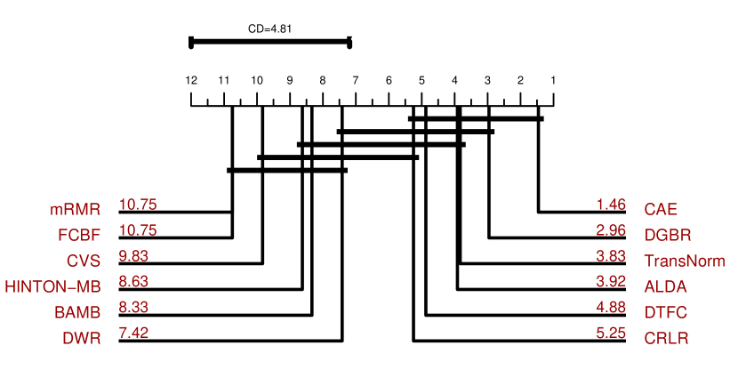
(a) Office-Caltech10

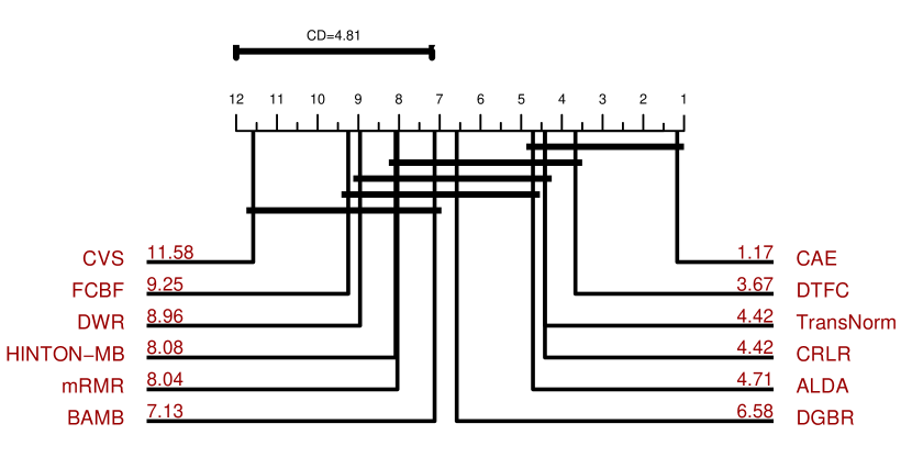
(b) Amazon Review

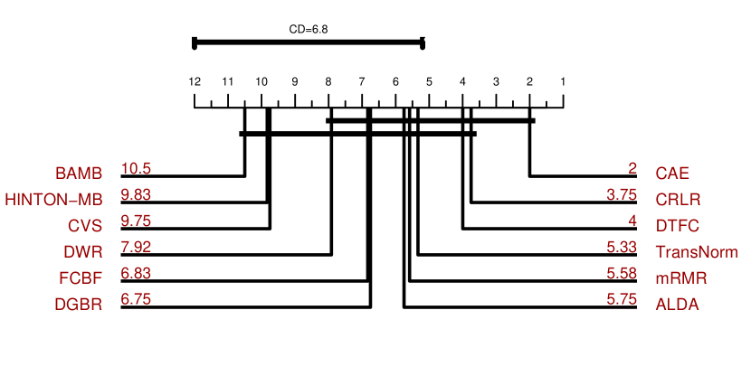
(c) Reuters-21578

Figure 2: Comparison of CAE against the other algorithms with the Nemenyi test. The lower rank value is better (lower ranks to the right).

4.2.2 Statistical Tests

To further compare the performance of CAE with that of its rivals, the Friedman test and Nemenyi test [46] are employed.

We first perform the Friedman test at the 5% significance level under the null-hypothesis which states that all algorithms are performing equivalently (i.e., the average ranks of all algorithms are equivalent). The average ranks of CAE and its rivals are summarized in the last column of Tables 1 to 3. It can be seen that the null hypothesis is rejected on all the three datasets. We also note that CAE performs better than its rivals (the lower rank value is better).

To further analyze the significant difference between CAE and its rivals, we perform the Nemenyi test. Based on the test, the performances of two algorithms are significantly different if the corresponding average ranks differ by at least one critical difference (CD). The CD for the Nemenyi test [46] is calculated as follows.

$${\rm CD}=q_{a,m}\sqrt{\frac{m(m+1)}{6|\mathcal{D}|}}$$

where $\alpha$ is the significance level and $m$ is the number of comparison models, and $|\mathcal{D}|$ denotes the number of cross-domain tasks. In our experiments, $m$ = 12, $q_{a=0.05,m=12}$ = 3.268 at significance level $\alpha$ = 0.05. On the Office-Caltech10 and Amazon Review datasets, $|\mathcal{D}|$ = 12, and thus CD = 4.81. On the Reuters-21578 dataset, $|\mathcal{D}|$ = 6, and thus CD = 6.80.

Fig.2 provides the CD diagrams, where the average rank of each algorithm is marked along the axis (lower ranks to the right). On the Office-Caltech10 dataset, CAE achieves comparable performance against DGBR, TransNorm, ALDA, DTFC and CRLR, and CAE significantly outperforms the other algorithms. On the Amazon Review dataset, CAE significantly outperforms CVS, FCBF, DWR, HINTON-MB, mRMR and BAMB, and CAE achieves comparable performance against the other algorithms. On the Reuters-21578 dataset, CAE significantly outperforms BAMB, HINTON-MB, CVS, DWR, FCBF and DGBR, and CAE achieves comparable performance against the other algorithms. CAE is the only algorithm that achieves the lowest ranking values in all three datasets.

4.3 Ablation and Sensitivity Analysis

To study the effect of different components of the objective function of CAE, we perform an ablation study on nine cross-domain tasks. To investigate the effect of the causal structure loss $\mathcal{L}_{C}$, we remove $\mathcal{L}_{C}$ from Eq.(1) and keep other components unchanged, and we denote this version of CAE as “CAE w/o $\mathcal{L}_{C}$”. To investigate the effect of the cross-entropy loss $\mathcal{L}_{Y}$, similarly we use the “CAE w/o $\mathcal{L}_{Y}$”, for which the $\mathcal{L}_{Y}$ component is removed from Eq.(1) while the other components remain unchanged. The experimental results are summarized in Table 4 to 6. We observe that “CAE w/o $\mathcal{L}_{C}$” is inferior to CAE, which indicates the effectiveness of the $\mathcal{L}_{C}$ component. On the tasks of A$\rightarrow$D and D$\rightarrow$C, “CAE w/o $\mathcal{L}_{C}$” achieves better results than CAE, but “CAE w/o $\mathcal{L}_{C}$” is inferior to CAE on the tasks of A$\rightarrow$C and D$\rightarrow$A, D$\rightarrow$W. The reason is that “CAE w/o $\mathcal{L}_{C}$” may capture spurious correlations between features and the class variable, as it does not use the $\mathcal{L}_{C}$ term to separate the learnt low-dimensional representations into two groups, the spurious correlations may facilitate the learning of the tasks of A$\rightarrow$D, W$\rightarrow$C and D$\rightarrow$C, but they may not be transferable across different target domains. Comparing the result of “CAE w/o $\mathcal{L}_{Y}$” and CAE, we note that the performance of “CAE w/o $\mathcal{L}_{Y}$” drops, which shows the necessity of incorporating the label information of source domain to improve the quality of causal representations for predictions. We can conclude that both causal structure loss $\mathcal{L}_{C}$ and cross-entropy loss $\mathcal{L}_{Y}$ play a major role in CAE.

Table 4: Ablation study on the Amazon Review dataset.

Methods	C$\rightarrow$A	C$\rightarrow$W	C$\rightarrow$D	A$\rightarrow$C	A$\rightarrow$W	A$\rightarrow$D	W$\rightarrow$C	W$\rightarrow$A	W$\rightarrow$D	D$\rightarrow$C	D$\rightarrow$A	D$\rightarrow$W	Avg
CAE w/o $\mathcal{L}_{C}$	50.96	38.64	43.82	41.76	36.20	38.73	37.31	38.18	80.89	33.74	33.79	76.54	45.88
CAE w/o $\mathcal{L}_{Y}$	45.72	37.96	44.59	35.26	32.20	32.48	30.45	35.38	73.24	32.94	34.24	71.52	42.17
CAE	52.36	39.66	45.54	43.46	38.30	35.66	37.40	39.56	83.44	33.39	34.86	78.64	46.86

Table 5: Ablation study on the Office-Caltech10 dataset.

Methods	B$\rightarrow$D	B$\rightarrow$E	B$\rightarrow$K	D$\rightarrow$B	D$\rightarrow$E	D$\rightarrow$K	E$\rightarrow$B	E$\rightarrow$D	E$\rightarrow$K	K$\rightarrow$B	K$\rightarrow$D	K$\rightarrow$E	Avg
CAE w/o $\mathcal{L}_{C}$	79.15	77.47	77.74	73.00	75.57	78.98	72.90	73.08	83.39	68.60	74.69	81.93	76.37
CAE w/o $\mathcal{L}_{Y}$	78.69	77.03	78.09	70.90	75.72	78.98	70.35	68.08	79.29	69.00	70.54	77.18	74.49
CAE	79.15	77.35	78.83	73.62	76.82	79.87	73.67	74.18	83.96	71.20	75.44	83.38	77.29

Table 6: Ablation study on the Reuters-21578 dataset.

Methods	Or$\rightarrow$Pe	Or$\rightarrow$Pl	Pe$\rightarrow$Pl	Pe$\rightarrow$Or	Pl$\rightarrow$Or	Pl$\rightarrow$Pe	Avg
CAE w/o $\mathcal{L}_{C}$	73.34	62.99	58.12	74.55	63.87	60.33	65.53
CAE w/o $\mathcal{L}_{Y}$	72.93	61.45	58.49	71.79	63.39	58.69	64.46
CAE	75.66	64.33	59.05	77.60	65.26	60.33	67.03

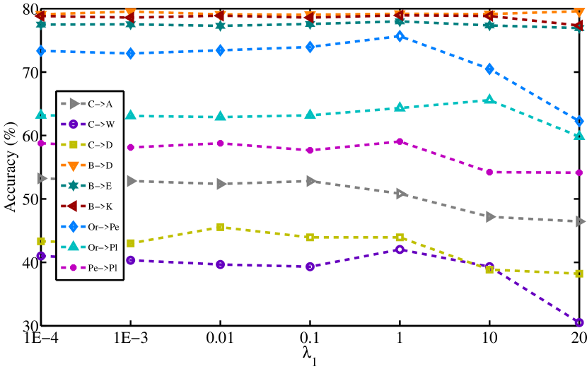
(a) Parameter $\lambda_{1}$

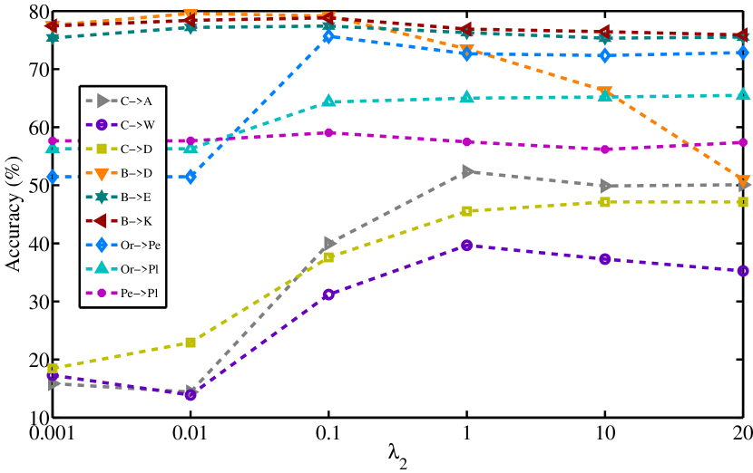
(b) Parameter $\lambda_{2}$

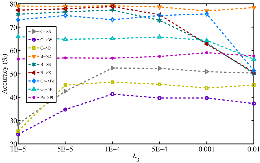
(c) Parameter $\lambda_{3}$

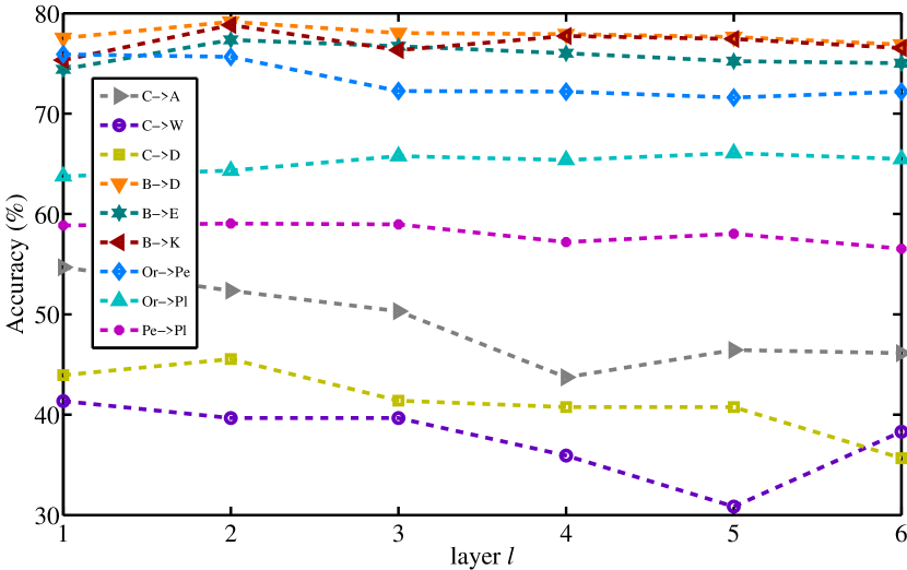
(d) Parameter $l$

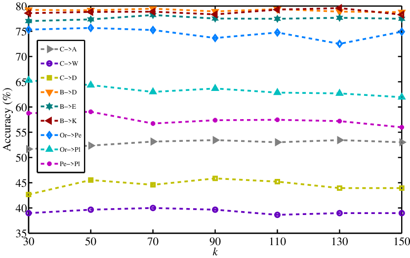
(e) Parameter $k$

Figure 3: Parameter sensitivity study for CAE on randomly selected cross-domain tasks.

We also investigate the sensitivity of CAE with respect to parameters. CAE has five parameters, the number of stacked layers $l$, the number of low-dimensional features $k$, hyper-parameters $\lambda_{1}$, $\lambda_{2}$ and $\lambda_{3}$. When tuning a specific parameter, the other parameters remain unchanged.

Parameters $\lambda_{1}$, $\lambda_{2}$ and $\lambda_{3}$. The classification accuracies with different values for $\lambda_{1}$, $\lambda_{2}$ and $\lambda_{3}$ are plotted in Fig.3(a)(b)(c). We note that CAE is sensitive to the three hyper-parameters. For $\lambda_{1}$, [1,10] and [0.01,1] are the optimal value ranges for Amazon Review and the other datasets, respectively. For $\lambda_{2}$, [0.1,1] is the optimal value range for all datasets. For $\lambda_{3}$, [5E-4,0.001] and [5E-5,1E-4] are the optimal value range for Reuters-21578 and the other datasets, respectively. The values of $\lambda_{1}$ and $\lambda_{2}$ should be neither too small nor too large. If the value of each of them is too large, the effect of other three components in Eq.(1) will be weakened. If the value of $\lambda_{1}$ is too small, the low-dimensional representations learnt with a deep autoencoder model cannot well split into two groups, i.e. causal representations and task-irrelevant representations. Since autoencoder is an unsupervised model, if the value of $\lambda_{2}$ is too small, the low-dimensional representations learnt with a deep autoencoder model may contain less causal representations and contain more task-irrelevant representations. This will lead to poor performance.

Parameters $l$ and $k$. We plot the classification accuracies with different values for $l$ and $k$ in Fig.3(d)(e). We observe that CAE is sensitive to the two hyper-parameters. For $l$, [1,3] is the optimal value range for all datasets. If the value of $l$ is too large, it will make the training process difficult and it is easy to cause over fitting, leading to performance degradation. The value of $k$ cannot be set too large. For $k$, [50,90] is the optimal value range for all datasets. If the value of $k$ continues to increase, the training time increases a lot but the performance drops.

5 Conclusion and Future Studies

In this paper, we study a new problem, robust domain adaptation, in which the unlabeled target domain data is unknown during the model training phase. To tackle this problem, we propose the Causal AutoEncoder (CAE) algorithm, which jointly optimizes a deep autoencoder model and a causal structure learning model to extract casual representations only using data from a single source domain. To the best of our knowledge, CAE is the first method to directly learn causal representations using a deep autoencoder model. Our method provides a new insight for learning causal representation using deep neural networks. Extensive experiments are conducted on three real-world datasets, and the experimental results demonstrate the effectiveness of our proposed method. Future work could study how to combine autoencoder and other deep neural networks to learn higher quality causal representations for robust domain adaptation.

Appendix

In this section, we will give a brief introduction to Markov Blanket (MB) [40]. Let U denote the set of random variables. $\mathbb{P}$ represents a joint probability distribution over U, and $\mathbb{G}$ is a directed acyclic graph (DAG) over U. In a DAG, if there exists a directed edge from variable X to variable Y, then X is a parent of Y and Y is a child of X. X is an ancestor of Y (i.e., non-descendant of Y) and Y is a descendant of X if there exists a directed path from X to Y. The triplet $<\emph{{U}},\mathbb{G},\mathbb{P}>$ constitutes a Bayesian Network (BN) if and only if $<\emph{{U}},\mathbb{G},\mathbb{P}>$ satisfies the Markov condition [41]: each variable is conditionally independent of variables in its non-descendants given its parents in $\mathbb{G}$. In the following, we will first give the definitions of conditional independence and faithfulness, then briefly introduce MB.

Definition 1 (Conditional Independence [40]).

Given a conditioning set Z, variable X is conditionally independent of variable Y if and only if $P(X|Y,\textbf{Z})=P(X|\textbf{Z})$.

Definition 2 (Faithfulness [41]).

Given a Bayesian Network $<\textbf{U},\mathbb{G},\mathbb{P}>$, $\mathbb{G}$ is faithful to $\mathbb{P}$ if and only if all the conditional independencies appear in $\mathbb{P}$ are entailed by $\mathbb{G}$. $\mathbb{P}$ is faithful if and only if there is a DAG $\mathbb{G}$ such that $\mathbb{G}$ is faithful to $\mathbb{P}$.

The notion of a Markov blanket (MB) was proposed by Pearl et al. [40] in the context of a Bayesian network (BN). If the faithfulness assumption (see Definition 2) holds in a BN, the MB of a target variable T consists of parents, children and spouses (other parents of the children) of T and is uniqueness, is denoted as MB_T (Definition 3). Fig. 4 gives an example of a MB in a BN. The MB of T includes A and B (parents), C and D (children), and E (spouse), that is, MB_T = {A, B, C, D, E}. The MB of a target variable is the minimal feature subset that renders all other features conditionally independent of the target (see Theorem 2). As shown in Fig.4, given conditioning set MB_T, variables F, I, Q, H and K all are conditionally independent of the target T. The MB of the class variable has been proved to be the optimal feature subset for feature selection under the faithfulness condition [37]. As a concept from Bayesian network (BN), the MB of class variable provides the local causal structure around the class variable and thus uncovers the causal relationships between features and the class variable [40]. Compared with non-causal feature selection considering exploit statistical associations or dependences between features and the class variable, causal feature selection uncovers the underlying mechanism of the occurrence of the class variable that is persistent across different settings or environments, and thus it has potential abilities to select more robust and interpretable features than non-causal feature selection methods in non-static environment. Recently, due to the interpretability and robustness, MB has received increasing attention and has been widely applied for causal feature selection [16].

Definition 3 (Markov Blanket [40]).

In a faithful BN, the MB of a target variable T is denoted as MB_T, which consists of parents, children and spouses (other parents of the children) of T and is uniqueness.

Theorem 2 [40].

Given the Markov blanket (MB_T) of a target variable T, all other variables in U $\setminus$MB_T$\setminus${T} are conditionally independent of T, that is, X $\!\perp\!\!\!\perp$ T $|$ MB_T, for $\forall$ X $\subseteq$ U $\setminus$MB_T$\setminus${T} .

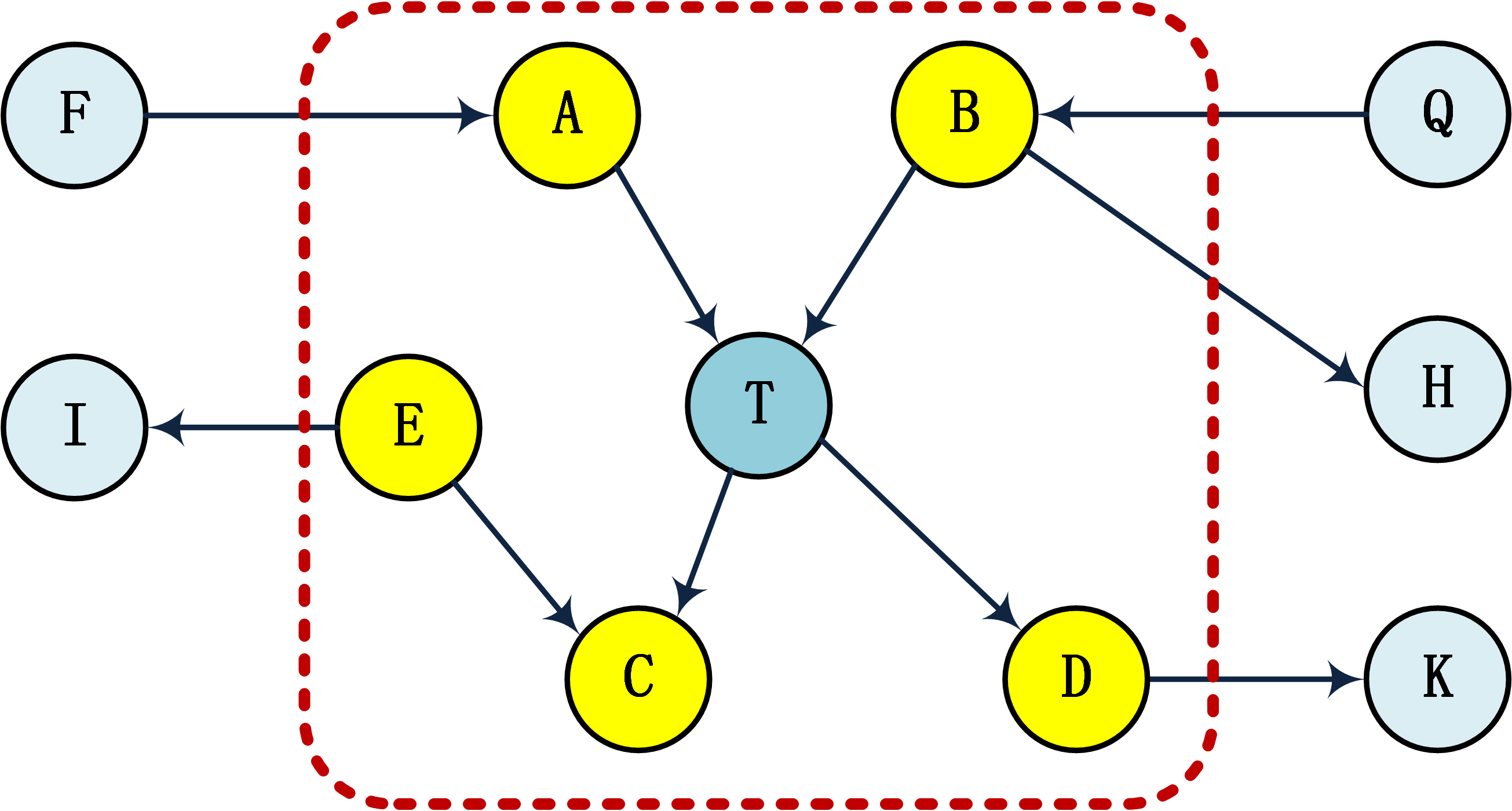
Figure 4: An example of an MB of variable T (yellow variables) in a Bayesian network.

REFERENCES

REFERENCES

- [1] F. Zhuang, Z. Qi, K. Duan, D. Xi, Y. Zhu, H. Zhu, H. Xiong, Q. He, A comprehensive survey on transfer learning, CoRR abs/1911.02685.
- [2] C. Ren, X. Xu, H. Yan, Generalized conditional domain adaptation: A causal perspective with low-rank translators, IEEE transactions on cybernetics 50 (2) (2020) 821–834.
- [3] Y. Chen, S. Song, S. Li, L. Yang, C. Wu, Domain space transfer extreme learning machine for domain adaptation, IEEE transactions on cybernetics 49 (5) (2019) 1909–1922.
- [4] P. Wei, Y. Ke, Knowledge transfer based on multiple manifolds assumption, in: Proceedings of the 28th ACM International Conference on Information and Knowledge Management, November 3-7, Beijing, China, 2019, pp. 279–287.
- [5] M. Chen, S. Zhao, H. Liu, D. Cai, Adversarial-learned loss for domain adaptation, in: Proceedings of the Thirty-Fourth AAAI Conference on Artificial Intelligence, February 7-12, New York, USA, 2020, pp. 3521–3528.
- [6] Z. Deng, Y. Luo, J. Zhu, Cluster alignment with a teacher for unsupervised domain adaptation, in: 2019 IEEE/CVF International Conference on Computer Vision, ICCV ,October 27 - November 2, Seoul, Korea (South),, 2019, pp. 9943–9952.
- [7] S. Li, C. H. Liu, B. Xie, L. Su, Z. Ding, G. Huang, Joint adversarial domain adaptation, in: Proceedings of the 27th ACM International Conference on Multimedia, October 21-25, Nice, France, 2019, pp. 729–737.
- [8] G. Kang, L. Jiang, Y. Yang, A. G. Hauptmann, Contrastive adaptation network for unsupervised domain adaptation, in: IEEE Conference on Computer Vision and Pattern Recognition, June 16-20, CA, USA, 2019, pp. 4893–4902.
- [9] M. Long, Z. Cao, J. Wang, M. I. Jordan, Conditional adversarial domain adaptation, in: Advances in Neural Information Processing Systems 31, December 3-8, Canada, 2018, pp. 1647–1657.
-
[10]
K. Zhang, M. Gong, P. Stojanov, B. Huang, C. Glymour,
Domain adaptation as a problem of
inference on graphical models, CoRR abs/2002.03278.
URL https://arxiv.org/abs/2002.03278 - [11] T. Teshima, I. Sato, M. Sugiyama, Few-shot domain adaptation by causal mechanism transfer, CoRR abs/2002.03497.
- [12] J. Wang, J. Jiang, Conditional coupled generative adversarial networks for zero-shot domain adaptation, in: IEEE/CVF International Conference on Computer Vision, ICCV, October 27 - November 2,Seoul, Korea (South),, IEEE, 2019, pp. 3374–3383.
- [13] K. Peng, Z. Wu, J. Ernst, Zero-shot deep domain adaptation, in: V. Ferrari, M. Hebert, C. Sminchisescu, Y. Weiss (Eds.), Computer Vision - ECCV 2018 - 15th European Conference, Munich, Germany, September 8-14, 2018, Proceedings, Part XI, Vol. 11215, pp. 793–810.
-
[14]
J. Wang, J. Jiang, Adversarial learning
for zero-shot domain adaptation, CoRR abs/2009.05214.
arXiv:2009.05214.
URL https://arxiv.org/abs/2009.05214 - [15] B. Schölkopf, Causality for machine learning, CoRR abs/1911.10500.
- [16] K. Yu, X. Guo, L. Liu, J. Li, H. Wang, Z. Ling, X. Wu, Causality-based feature selection: Methods and evaluations, ACM Computing Surveys (CSUR) 53 (5) (2020) 1–36.
- [17] K. Kuang, B. Li, P. Cui, Y. Liu, J. Tao, Y. Zhuang, F. Wu, Stable prediction via leveraging seed variable, CoRR abs/2006.05076.
- [18] Z. Ling, K. Yu, H. Wang, L. Liu, W. Ding, X. Wu, BAMB: A balanced markov blanket discovery approach to feature selection, ACM Trans. Intell. Syst. Technol. 10 (5) (2019) 52:1–52:25.
- [19] T. Gao, Q. Ji, Efficient score-based markov blanket discovery, Int. J. Approx. Reason. 80 (2017) 277–293.
- [20] S. Li, C. H. Liu, Q. Lin, B. Xie, Z. Ding, G. Huang, J. Tang, Domain conditioned adaptation network, in: The Thirty-Fourth AAAI Conference on Artificial Intelligence, February 7-12, New York, NY, USA, 2020, pp. 11386–11393.
- [21] S. Yang, H. Wang, Y. Zhang, P. Li, Y. Zhu, X. Hu, Semi-supervised representation learning via dual autoencoders for domain adaptation, Knowl. Based Syst. 190 (2020) 105161.
- [22] P. Wei, Y. Ke, C. K. Goh, Feature analysis of marginalized stacked denoising autoenconder for unsupervised domain adaptation, IEEE transactions on neural networks and learning systems 30 (5) (2019) 1321–1334.
- [23] S. Yang, Y. Zhang, H. Wang, P. Li, X. Hu, Representation learning via serial robust autoencoder for domain adaptation, Expert Systems with Applications. (2020) 113635.
- [24] S. Yang, Y. Zhang, Y. Zhu, P. Li, X. Hu, Representation learning via serial autoencoders for domain adaptation, Neurocomputing 351 (2019) 1–9.
- [25] X. Wang, Y. Jin, M. Long, J. Wang, M. I. Jordan, Transferable normalization: Towards improving transferability of deep neural networks, in: Advances in Neural Information Processing Systems 32: Annual Conference on Neural Information Processing Systems, Vancouver, BC, Canada, December 8-14, 2019, pp. 1951–1961.
- [26] M. Ghifary, W. B. Kleijn, M. Zhang, D. Balduzzi, Domain generalization for object recognition with multi-task autoencoders, in: 2015 IEEE International Conference on Computer Vision, ICCV 2015, Santiago, Chile, December 7-13, 2015, 2015, pp. 2551–2559.
- [27] H. Li, S. J. Pan, S. Wang, A. C. Kot, Domain generalization with adversarial feature learning, in: 2018 IEEE Conference on Computer Vision and Pattern Recognition, CVPR 2018, Salt Lake City, UT, USA, June 18-22, 2018, 2018, pp. 5400–5409.
- [28] Q. Dou, D. C. de Castro, K. Kamnitsas, B. Glocker, Domain generalization via model-agnostic learning of semantic features, in: Advances in Neural Information Processing Systems 32: Annual Conference on Neural Information Processing Systems 2019, NeurIPS 2019, December 8-14, Vancouver, BC, Canada, 2019, pp. 6447–6458.
- [29] S. Magliacane, T. van Ommen, T. Claassen, S. Bongers, P. Versteeg, J. M. Mooij, Domain adaptation by using causal inference to predict invariant conditional distributions, in: Advances in Neural Information Processing Systems 31, December 3-8, Canada, 2018, pp. 10869–10879.
- [30] M. Rojas-Carulla, B. Schölkopf, R. E. Turner, J. Peters, Invariant models for causal transfer learning, J. Mach. Learn. Res. 19 (2018) 36:1–36:34.
- [31] K. Kuang, P. Cui, S. Athey, R. Xiong, B. Li, Stable prediction across unknown environments, in: Proceedings of the 24th ACM SIGKDD International Conference on Knowledge Discovery & Data Mining, KDD 2018, August 19-23, London, UK, 2018, pp. 1617–1626.
- [32] Z. Shen, P. Cui, T. Zhang, K. Kuang, Stable learning via sample reweighting, in: The Thirty-Fourth AAAI Conference on Artificial Intelligence, AAAI 2020, February 7-12, New York, USA,, 2020, pp. 5692–5699.
- [33] Z. Shen, P. Cui, K. Kuang, B. Li, P. Chen, Causally regularized learning with agnostic data selection bias, in: 2018 ACM Multimedia Conference on Multimedia Conference, MM 2018, October 22-26, Seoul, Republic of Korea, 2018, pp. 411–419.
- [34] K. Kuang, R. Xiong, P. Cui, S. Athey, B. Li, Stable prediction with model misspecification and agnostic distribution shift, in: The Thirty-Fourth AAAI Conference on Artificial Intelligence, February 7-12, New York, NY, USA, 2020, pp. 4485–4492.
- [35] L. Yu, H. Liu, Efficient feature selection via analysis of relevance and redundancy, J. Mach. Learn. Res. 5 (2004) 1205–1224.
- [36] H. Peng, F. Long, C. H. Q. Ding, Feature selection based on mutual information: Criteria of max-dependency, max-relevance, and min-redundancy, IEEE Trans. Pattern Anal. Mach. Intell. 27 (8) (2005) 1226–1238.
- [37] I. Tsamardinos, C. F. Aliferis, Towards principled feature selection: Relevancy, filters and wrappers, in: C. M. Bishop, B. J. Frey (Eds.), Proceedings of the Ninth International Workshop on Artificial Intelligence and Statistics, AISTATS 2003, Key West, Florida, USA, January 3-6, 2003.
- [38] C. F. Aliferis, I. Tsamardinos, A. R. Statnikov, HITON: A novel markov blanket algorithm for optimal variable selection, in: AMIA 2003, American Medical Informatics Association Annual Symposium, Washington, DC, USA, November 8-12, 2003, 2003.
- [39] T. Niinimaki, P. Parviainen, Local structure discovery in bayesian networks, in: Proceedings of the Twenty-Eighth Conference on Uncertainty in Artificial Intelligence, Catalina Island, CA, USA, 14-18 August, 2012, pp. 634–643.
- [40] J. Pearl, Probabilistic reasoning in intelligent systems: networks of plausible inference, Morgan Kaufmann series in representation and reasoning, 1988.
- [41] P. Spirtes, C. Glymour, R. Scheines, Causation, Prediction, and Search, MIT Press, 2000.
- [42] X. Zheng, B. Aragam, P. Ravikumar, E. P. Xing, Dags with NO TEARS: continuous optimization for structure learning, in: Advances in Neural Information Processing Systems 31: Annual Conference on Neural Information Processing Systems, December 3-8, Montréal, Canada, 2018, pp. 9492–9503.
- [43] B. Sun, J. Feng, K. Saenko, Return of frustratingly easy domain adaptation, in: D. Schuurmans, M. P. Wellman (Eds.), Proceedings of the Thirtieth AAAI Conference on Artificial Intelligence, February 12-17, Phoenix, Arizona, USA, 2016, pp. 2058–2065.
- [44] J. Wang, Y. Chen, H. Yu, M. Huang, Q. Yang, Easy transfer learning by exploiting intra-domain structures, in: IEEE International Conference on Multimedia and Expo, July 8-12, Shanghai, China, 2019, pp. 1210–1215.
- [45] Y. Cao, M. Long, J. Wang, Unsupervised domain adaptation with distribution matching machines, in: Proceedings of the Thirty-Second AAAI Conference on Artificial Intelligence, February 2-7, New Orleans, USA, 2018, pp. 2795–2802.
- [46] J. Demsar, Statistical comparisons of classifiers over multiple data sets, J. Mach. Learn. Res. 7 (2006) 1–30.