On a family of gradient type projection methods for nonlinear ill-posed problems

Abstract

We propose and analyze a family of successive projection methods whose step direction is the same as Landweber method for solving nonlinear ill-posed problems that satisfy the Tangential Cone Condition (TCC). This family enconpasses Landweber method, the minimal error method, and the steepest descent method; thush providing an unified framework for the analysis of these methods. Moreover, we define in this family new methods which are convergent for the constant of the TCC in a range twice as large as the one required for the Landweber and other gradient type methods.

The TCC is widely used in the analysis of iterative methods for solving nonlinear ill-posed problems. The key idea in this work is to use the TCC in order to construct special convex sets possessing a separation property, and to succesively project onto these sets.

Numerical experiments are presented for a nonlinear 2D elliptic parameter identification problem, validating the efficiency of our method.

Keywords. Nonlinear equations; Ill-posed problems; Projection methods; Tangential cone condition.

AMS Classification: 65J20, 47J06.

1 Introduction

In this article we propose a family of succesive orthogonal projection methods for obtaining stable approximate solutions to nonlinear ill-posed operator equations.

The inverse problems we are interested in consist of determining an unknown quantity $x\in X$ from the data set $y\in Y$, where $X$, $Y$ are Hilbert spaces. The problem data $y$ are obtained by indirect measurements of the parameter $x$, this process being described by the model $F(x)=y$, where $F:D\subset X\to Y$ is a non-linear ill-posed operator with domain $D=D(F)$.

In practical situations, the exact data $y$ is not known. Instead, what is available is only approximate measured data $y^{\delta}\in Y$ satisfying

$$\|y^{\delta}-y\|\leq\delta\,,$$ (1)

where $\delta>0$ is the noise level. Thus, the abstract formulation of the inverse problems under consideration is to find $x\in D$ such that

$$F(x)\ =\ y^{\delta}\,.$$ (2)

Standard methods for obtaining stable solutions of the operator equation in (2) can be divided in two major groups, namely, Iterative type regularization methods [1, 6, 7, 11, 12] and Tikhonov type regularization methods [6, 18, 24, 25, 26, 22]. A classical and general condition commonly used in the convergence analysis of these methods is the Tangent Cone Condition (TCC) [7].

In this work we use the TCC to define convex sets containing the local solutions of (2) and devise a family of succesive projection methods. The use of projection methods for solving linear ill-posed problems dates back to the 70’s (with the seminal works of Frank Natterer and Gabor Herman) [19, 20, 8, 9]. The combination of Landweber iterations with projections onto a feasible set, for solving (2) with $y^{\delta}$ in a convex set was analyzed in [5] (see also [6] and the references therein).

The distinctive features of the family of methods prposed in this work are as follows:

• the basic method in this family outperformed, in our preliminary numerical experiments, the classical Landweber iteration [7] as well as the steepest descent iteration [21] (with respect to both the computational cost and the number of iterations);

• the family is generated by introducing relaxation in the stepsize of the basic method and such a family encompasses, as particular cases, the Landweber method, the steepest descent method, as well as the minimal error method [21]; thus, providing an unified framework for their convergence analysis;

• the basic method within the family converges for the constant in the TCC twice as large as required for the convergence of the Landweber and other gradient type methods.

In view of theses features, the basic method within the proposed family is called Projected Landweber (PLW) method. Although in the linear case the PLW method coincides with the minimal error method, in the nonlinear case these two methods are distinct.

Landweber iteration was originally proposed for solving linear equations by using the method of successive approximations applied to the normal equations [12]. Its extension to non-linear equations was obtained substituting the adjoint of the linear map by the Jacobian’s adjoint of the operator under consideration [7]. Such a method is named (nonlinear) Landweber, in the setting of ill-posed problems. Convergence of this method in the nonlinear case under the TCC was proven by Hanke et al. [7]. Convergence analysis for the steepest descent method and minimal error method (in the nonlinear case) can be found in [21].

Although Levenberg-Marquardt type methods are faster than gradient type methods, with respect to the number of iterations, gradient type methods have simpler and faster iteration formulas. Moreover, they fit nicely in Cimino and Kaczmarz type schemes. For these reasons, acceleration of gradient type methods is a relevant topic in the field of ill-posed problems.

The article is outlined as follows. In Section 2 we state the main assumptions and derive some auxiliary estimates required for the analysis of the proposed family of methods. In Section 3 we define the convex sets $H_{x}$ (6), prove a special separation property (Lemma 3.1) and introduce our family of methods (8). Moreover, the first convergence analysis results are obtained, namely: monotonicity (Proposition 3.2) and strong convergence (Theorems 3.3 and 3.4) for the exact data case. In Section 4 we consider the noisy data case ($\delta>0$). The convex sets $H_{x}^{\delta}$ are defined and another separation property is derived (Lemma 4.1). The discrepancy principle is used to define a stopping criteria (20), which is proved to be finite (Theorem 4.3). Monotonicity is proven (Proposition 4.2) as well as a stability result (Theorem 4.4) and a norm convergence result (Theorem 4.5). Section 5 is devoted to numerical experiments. In Section 6 we present final remarks and conclusions.

2 Main assumptions and preliminary results

In this section we state our main assumptions and discuss some of their consequences, which are relevant for the forthcoming analysis. To simplify the notation, from now on we write

$$F_{\delta}(x)\ :=\ F(x)-y^{\delta}\quad\quad{\rm and}\quad\quad F_{0}(x)\ :=\ F(x)-y\,.$$ (3)

Throughout this work we make the following assumptions, which are frequently used in the analysis of iterative regularization methods (see, e.g., [6, 11, 22]):

A1

$F$ is a continuous operator defined on $D(F)\subset X$, which has nonempty interior. Moreover, there exist constants $C$, $\rho>0$ and $x_{0}\in D(F)$ such that $F^{\prime}$, the Gateaux derivative of $F$, is defined on $B_{\rho}(x_{0})$ and satisfies

$$\|F^{\prime}(x)\|\ \leq\ C\,,\quad\ x\in B_{\rho}(x_{0})\subset D(F)$$ (4)

(the point $x_{0}$ is be used as initial guess for our family of methods).

A2

The local tangential cone condition (TCC) [6, 11]

$$\|F(\bar{x})-F(x)-F^{\prime}(x)(\bar{x}-x)\|_{Y}\ \leq\ \eta\|F(\bar{x})-F(x)\|_{Y}\,,\quad\forall\ x,\bar{x}\in B_{\rho}(x_{0})$$ (5)

holds for some $\eta<1$, $x_{0}\in X$, and $\rho>0$.

A3

There exists an element $x^{\star}\in B_{\rho/2}(x_{0})$ such that $F(x^{\star})=y$, where $y\in Rg(F)$ are the exact data satisfying (1).

A4

The operator $F$ is continuously Fréchet differentiable on $B_{\rho}(x_{0})$.

Observe that in the TCC we require $\eta<1$, instead of $\eta<1/2$ as in classical convergence analysis for the nonlinear Landweber under this condition [6]. The TCC (5) represents a uniform assumption (on a ball of radius $\rho$) on the non-linearity of the operator $F$, and has interesting consequences (see [6, pg.278–280] or [11, pg.6 and Sec.2.4 (pg.26–29)]). Here we discuss some of them.

Proposition 2.1.

If A1 and A2 hold, then for any $x$, $\bar{x}\in B_{\rho}(x_{0})$

1. $(1-\eta)\|F(x)-F(\bar{x})\|\leq\|F^{\prime}(x)(x-\bar{x})\|\leq(1+\eta)\|F(x)-F(\bar{x})\|$;

2. $\langle F^{\prime}({x})^{*}F_{0}({x}),{x}-\bar{x}\rangle\leq(1+\eta)(\|F_{0}(x)\|^{2}+\|F_{0}(x)\|\|F_{0}(\bar{x})\|)$;

3. $\langle F^{\prime}({x})^{*}F_{0}({x}),{x}-\bar{x}\rangle\geq(1-\eta)\|F_{0}({x})\|^{2}-(1+\eta)\|F_{0}({x})\|\|F_{0}(\bar{x})\|$.

If, additionally, $F_{0}(x)\neq 0$ then

$$(1-\eta)\|F_{0}(x)\|-(1+\eta)\|F_{0}(\bar{x})\|\\ \leq\ \|F^{\prime}(x)^{*}(x-\bar{x})\|\ \leq\ (1+\eta)(\|F_{0}(x)\|+\|F_{0}(\bar{x})\|).$$

Proof.

Item 1 follows immediately from the TCC and the triangle inequality, as proved in [6, Eq.(11.7)].

Direct algebraic manipulations yield

$$\langle F^{\prime}(x)^{*}F(x),x-\bar{x}\rangle\ =\ \langle F(x),F^{\prime}(x)(x-\bar{x})\rangle\\ \leq\ (1+\eta)\|F(x)\|\|F(x)-F(\bar{x})\|\,,$$

where the inequality follows from Cauchy-Schwarz inequality and item 1. Likewise,

$$\langle F^{\prime}({x})^{*} F_{0}({x}),\,{x}-\bar{x}\rangle\ =\ \langle F_{0}({x}),F^{\prime}({x})({x}-\bar{x})\rangle$$

$$=\ \langle F_{0}({x}),F_{0}({x})-F_{0}(\bar{x})\rangle+\langle F_{0}({x}),F_{0}(\bar{x})-F_{0}(x)-F^{\prime}(x)(\bar{x}-x)\rangle$$

$$\geq\ \|F_{0}({x})\|^{2}-\|F_{0}({x})\|\|F_{0}(\bar{x})\|-\eta\|F_{0}({x})\|\|F_{0}({x})-F_{0}(\bar{x})\|\,,$$

where the inequality follows from Cauchy-Schwarz inequality and the first inequality in this proof. Items 2 and 3 follow from the above inequalities and the inequality $\|F_{0}(x)-F_{0}(\bar{x})\|\leq\|F_{0}(x)\|+\|F_{0}(\bar{x})\|$. ∎

The next result relates to the solvability of operator equation $F(x)=y$ with exact data.

Proposition 2.2.

Let A1 – A3 be satisfied. For any $x\in B_{\rho}(x_{0})$, $F_{0}(x)=0$ if and only if $F^{\prime}(x)^{*}F_{0}(x)=0$. Moreover, for any $(x_{k})\in B_{\rho}(x_{0})$ converging to some $\bar{x}\in B_{\rho}(x_{0})$, the following statements are equivalent:

a)  $\lim\limits_{k\to\infty}\|F^{\prime}(x_{k})^{*}F_{0}(x_{k})\|\,=\,0$;   b)  $\lim\limits_{k\to\infty}\|F_{0}(x_{k})\|\,=\,0$;   c) $F(\bar{x})\,=\,y$.

Proof.

See [11, pg. 279] for a proof of the first statement. For proving the second statement:
the implication $(b)\Rightarrow(a)$ follows from A1 and the hypothesis $(x_{k})\in B_{\rho}(x_{0})$; on the other hand, $(a)\Rightarrow(b)$ follows from Proposition 2.1, item 3 with $x=x_{k}$ and $\bar{x}=x^{\star}$; moreover, $(b)\Rightarrow(c)$ and $(b)\Leftarrow(c)$ follow from the hypothesis  $\lim\limits_{k\to\infty}\|x_{k}-\bar{x}\|=0$ and A1. ∎

Notice that the equivalence between $(a)$ and $(b)$ in Proposition 2.2 does not depend on the convergence of sequence $(x_{k})$. The next result provides a convenient way of rewriting the TCC (5) for $\bar{x}=x^{\star}\in F^{-1}(y)$ using notation (3).

Proposition 2.3.

Let A2 be satisfied. If $x^{\star}\in B_{\rho}(x_{0})\cap F^{-1}(y)$ then

$$\|y-y^{\delta}-F_{\delta}(x)-F^{\prime}(x)(x^{\star}-x)\|\ \leq\ \eta\,\|y-y^{\delta}-F_{\delta}(x)\|,\quad\forall x\in B_{\rho}(x_{0}).$$

3 A family of relaxed projection Landweber methods

In this section we assume that exact data $y^{\delta}=y\in$ Rg$(F)$ are available, introduce a family of relaxed projection Landweber methods for the exact data case, and prove their convergence.

Define, for each $x\in D(F)$, the set

$$H_{x}\ :=\ \{z\in X\;|\;\langle z-x,F^{\prime}(x)^{*}F_{0}(x)\rangle\leq-(1-\eta)\|F_{0}(x)\|^{2}\}\,.$$ (6)

Note that $H_{x}$ is either $\emptyset$, a closed half-space, or $X$. As we prove next, $H_{x}$ has an interesting geometric feature: it contains all exact solutions of (2) in $B_{\rho}(x_{0})$ and, whenever $x$ is not a solution of (2), it does not contain $x$.

Lemma 3.1 (Separation).

Let A1 and A2 be satisfied. If $x\in B_{\rho}(x_{0})$ then

$$0\ \geq\ (1-\eta)\|F_{0}(x)\|^{2}+\langle F^{\prime}(x)^{*}F_{0}(x),x^{\star}-x\rangle\,,\quad\forall x^{\star}\in B_{\rho}(x_{0})\cap F^{-1}(y)\,.$$ (7)

Consequently,

1.  $B_{\rho}(x_{0})\cap F^{-1}(y)\subset H_{x}$; 2.  $x\in H_{x}\iff F(x)=y$.

Proof.

The first statement follows trivially from Proposition 2.1 item 3 with $\bar{x}=x^{\star}\in B_{\rho}(x_{0})\cap F^{-1}(y)$. Items 1 and 2 are immediate consequences of the first statement and Definition (6). ∎

We are now ready to introduce our family of relaxed projection Landweber methods. Choose $x_{0}\in X$ according to A2 and A3 and define, for $k\geq 0$, the sequence

$$x_{k+1}:=x_{k}-\theta_{k}\,\lambda_{k}\,F^{\prime}(x_{k})^{*}F_{0}(x_{k}),$$ (8a)

$$\text{where }\theta_{k}\in(0,2),\;\lambda_{k}:=\begin{cases}0,&\text{if }F^{\prime}(x_{k})^{*}F_{0}(x_{k})=0\\ \dfrac{(1-\eta)\|F_{0}(x_{k})\|^{2}}{\|F^{\prime}(x_{k})^{*}F_{0}(x_{k})\|^{2}},&\text{otherwise.}\end{cases}$$ (8b)

In view of definition (6), the orthogonal projection of $x_{k}$ onto $H_{x_{k}}$ is $\hat{x}=x_{k}-\lambda_{k}F^{\prime}(x_{k})^{*}F_{0}(x_{k})$ so that

$$x_{k+1}=x_{k}+\theta_{k}(\hat{x}-x_{k})=(1-\theta_{k})x_{k}+\theta_{k}\hat{x}\,.$$

We define the PLW method as (8) with $\theta_{k}=1$ for all $k$. This choice amounts to taking $x_{k+1}$ as the orthogonal projection of $x_{k}$ onto $H_{x_{k}}$. The family of relaxed projection Landweber methods is obtained by choosing $\theta_{k}\in(0,2)$, which is equivalent to taking $x_{k+1}$ as a relaxed orthogonal projection of $x_{k}$ onto $H_{x_{k}}$.

Iteration (8) is well defined for all $x_{k}\in D(F)$; due to Proposition 2.2, this iteration becomes stationary at $x_{\tilde{k}}\in B_{\rho}(x_{0})$, i.e. $x_{k}=x_{\tilde{k}}$ for $k\geq\tilde{k}$, if and only if $F(x_{\tilde{k}})=y$.

In the next proposition an inequality is established, that guarantees the monotonicity of the iteration error for the family of relaxed projection Landweber methods in the case of exact data, i.e., $\|x^{\star}-x_{k+1}\|\leq\|x^{\star}-x_{k}\|$, whenever $\theta_{k}\in(0,2)$.

Proposition 3.2.

Let A1 – A3 hold true. If $x_{k}\in B_{\rho}(x_{0})$, $F^{\prime}(x_{k})^{*}F(x_{k})\neq 0$, and $\theta_{k}$ and $x_{k+1}$ are as in (8), then

$$\|x^{\star}-x_{k}\|^{2}\ \geq\ \|x^{\star}-x_{k+1}\|^{2}+\theta_{k}\,(2-\theta_{k})\left((1-\eta)\dfrac{\|F_{0}(x_{k})\|^{2}}{\|F^{\prime}(x_{k})^{*}F_{0}(x_{k})\|}\right)^{2},$$

for all $x^{\star}\in B_{\rho}(x_{0})\cap F^{-1}(y)$.

Proof.

If $x_{k}\in B_{\rho}(x_{0})$ and $F^{\prime}(x_{k})^{*}F(x_{k})\neq 0$ then $x_{k+1}$ is a relaxed orthogonal projection of $x_{k}$ onto the $H_{x_{k}}$ with a relaxation factor $\theta_{k}$. The conclusion follows from this fact, Lemma 3.1, iteration formula (8) and the properties of relaxed metric projections onto arbitrary sets (see, e.g., [27, Lemma 3.13, pp. 21–22].) ∎

Direct inspection of the inequality in Proposition 3.2 shows that the choice $\theta_{k}\in(0,2)$, as prescribed in (8), guarantees decrease of the iteration error $\|x^{\star}-x_{k}\|$, while $\theta_{k}=1$ yields the greatest estimated decrease on the iteration error.

We are now ready to state and prove the main results of this section: Theorem 3.3 gives a sufficient condition for strong convergence of the family of relaxed projection Landweber methods (for exact data) to some point $\bar{x}\in B_{\rho}(x_{0})$. Theorem 3.4 gives a sufficient condition for strong convergence of this family of methods to a solution of $F(x)=y$, shows that steepest descent, minimal error, as well as Landweber method are particular instances of methods belonging to this family, and proves convergence of these three methods within this framework.

Recall that the steepest descent method (SD) is given by

$$x_{x+1}\ =\ x_{k}-\dfrac{\|F^{\prime}(x_{k})^{*}F_{0}(x_{k})\|^{2}}{\|F^{\prime}(x_{k})F^{\prime}(x_{k})^{*}F_{0}(x_{k})\|^{2}}\,F^{\prime}(x_{k})^{*}F_{0}(x_{k})\,,$$

while the minimal error method (ME) is given by

$$x_{x+1}\ =\ x_{k}-\dfrac{\|F_{0}(x_{k})\|^{2}}{\|F^{\prime}(x_{k})^{*}F_{0}(x_{k})\|^{2}}\,F^{\prime}(x_{k})^{*}F_{0}(x_{k})\,.$$

Theorem 3.3.

If A1 – A3 hold true, then the sequences $(x_{k})$, $(\theta_{k})$ as specified in (8) are well defined and

$$x_{k}\in B_{\rho/2}(x^{\star})\subset B_{\rho}(x_{0})\,,\ \forall\ k\in\mathbb{N}\,.$$ (9)

If, additionally, $\sup\,\theta_{k}<2$, then

$$(1-\eta)^{2}\sum_{k=0}^{\infty}\theta_{k}\dfrac{\|F_{0}(x_{k})\|^{4}}{\|F^{\prime}(x_{k})^{*}F_{0}(x_{k})\|^{2}}<\ \infty$$ (10)

and $(x_{k})$ converges strongly to some $\bar{x}\in B_{\rho}(x_{0})$.

Theorem 3.4.

Let A1 – A3 hold true, and the sequences $(x_{k})$, $(\theta_{k})$ be defined as in (8). The following statements hold:

a) If  $\inf$ $\theta_{k}>0$  and  $\sup$ $\theta_{k}<2$, then $(x_{k})$ converges to some $\bar{x}\in B_{\rho}(x_{0})$ solving $F(\bar{x})=y$.

b) If A2 holds with $\eta<1/2$ and

$$\theta_{k}:=(1-\eta)^{-1}\frac{\|F^{\prime}(x_{k})^{*}F_{0}(x_{k})\|^{2}}{\|F_{0}(x_{k})\|^{2}}\cdot\frac{\|F^{\prime}(x_{k})^{*}F_{0}(x_{k})\|^{2}}{\|F^{\prime}(x_{k})F^{\prime}(x_{k})^{*}F_{0}(x_{k})\|^{2}},$$

then $0<\theta_{k}\leq(1-\eta)^{-1}<2$, iteration (8) reduces to the steepest descent method and $(x_{k})$ converges to some $\bar{x}\in B_{\rho}(x_{0})$ solving $F(\bar{x})=y$.

c) If A1 and A2 hold with $C\leq 1$ and $\eta<1/2$, respectively, and

$$\theta_{k}:=(1-\eta)^{-1}\frac{\|F^{\prime}(x_{k})^{*}F_{0}(x_{k})\|^{2}}{\|F_{0}(x_{k})\|^{2}},$$

then $0<\theta_{k}\leq(1-\eta)^{-1}<2$, iteration (8) reduces to the nonlinear Landweber iteration and $(x_{k})$ converges to some $\bar{x}\in B_{\rho}(x_{0})$ solving $F(\bar{x})=y$.

d) If A1 and A2 hold with $C\leq 1$ and $\eta<1/2$, respectively, and $\theta_{k}:=(1-\eta)^{-1}$, then iteration (8) reduces to the nonlinear minimal error method and $(x_{k})$ converges to some $\bar{x}\in B_{\rho}(x_{0})$ solving $F(\bar{x})=y$.

Proof.

(Theorem 3.3) Assumption A3 guarantees the existence of $x^{\star}\in B_{\rho/2}(x_{0})$, a solution of $F(x)=y$. It follows from A3 that (9) holds for $k=0$. Suppose that the sequence $(x_{k})$, is well defined up to $k_{0}$ and that (9) holds for $k=k_{0}$. It follows from A1 that $x_{k_{0}}\in D(F)$, so that $x_{k_{0}+1}$ is well defined while it follows from (8) and Proposition 3.2 that (9) also holds for $k=k_{0}+1$.

To prove the second part of the theorem, suppose that $b:=\sup\theta_{k}<2$. At this point we have to consider two separate cases:
Case I:  $F(x_{\tilde{k}})=y$ for some $\tilde{k}\in\mathbb{N}$.
It follows from (9), Proposition 2.2 and (8), that $x_{j}=x_{\tilde{k}}$ for $j\geq\tilde{k}$, and we have trivially strong convergence of $(x_{k})$ to $\bar{x}=x_{\tilde{k}}$ (which, in this case, is a solution of $F(x)=y$).
Case II:  $F(x_{k})\neq y$, for all $k$.
It follows from (9) and Proposition 2.2 that $F^{\prime}(x_{k})^{*}F_{0}(x_{k})\neq 0$ for all $k$. According to (8b)

$$\lambda_{k}\,:=\,(1-\eta)\,\|F_{0}(x_{k})\|^{2}\,\|F^{\prime}(x_{k})^{*}F_{0}(x_{k})\|^{-2}.$$ (11)

Since $0<\theta_{k}\leq b<2$ for all $k$, $(2-\theta_{k})\theta_{k}\geq(2-b)\theta_{k}>0$, for all $k$. Therefore, it follows from Proposition 3.2 that

$$\|x^{\star}-x_{k}\|^{2}+(2-b)\,\theta_{k}\,(1-\eta)^{2}\sum_{j=0}^{k-1}\left(\dfrac{\|F_{0}(x_{j})\|^{2}}{\|F^{\prime}(x_{j})^{*}F_{0}(x_{j})\|}\right)^{2}\ \leq\ \|x^{\star}-x_{0}\|^{2},$$

for all $x^{\star}\in B_{\rho}(x_{0})\cap F^{-1}(y)$ and all $k\geq 1$. Consequently, using the definition of $\lambda_{k}$, we obtain

$$(1-\eta)^{2}\sum_{k=0}^{\infty}\theta_{k}\dfrac{\|F_{0}(x_{k})\|^{4}}{\|F^{\prime}(x_{k})^{*}F_{0}(x_{k})\|^{2}}\ =\ (1-\eta)\sum_{k=0}^{\infty}\theta_{k}\lambda_{k}\|F_{0}(x_{k})\|^{2}\ <\ \infty\,,$$ (12)

which, in particular, proves (10).

If $\sum\theta_{k}\lambda_{k}<\infty$ then $\sum\|x_{k}-x_{k+1}\|<\infty$ (due to (8a) and A1) and $(x_{k})$ is a Cauchy sequence.

Suppose that $\sum\theta_{k}\lambda_{k}=\infty$. It follows from (12) that $\lim\inf\|F_{0}(x_{k})\|=0$. Since we are in Case II, the sequence $(\|F_{0}(x_{k})\|)$ is strictly positive and there exists a subsequence $(x_{\ell_{i}})$ satisfying

$$0\leq k\leq\ell_{i}\ \Rightarrow\ \|F_{0}(x_{k})\|\ \geq\ \|F_{0}(x_{\ell_{i}})\|\,.$$ (13)

For all $k\in\mathbb{N}$ and $z\in B_{\rho}(x_{0})$,

$$\|x_{k}-z\|^{2} =\|x_{k+1}-z\|^{2}-\|x_{k}-x_{k+1}\|^{2}-2\langle x_{k}-x_{k+1},x_{k}-z\rangle$$

$$\leq\|x_{k+1}-z\|^{2}-2\langle x_{k}-x_{k+1},x_{k}-z\rangle$$

$$=\|x_{k+1}-z\|^{2}+2\theta_{k}\lambda_{k}\langle F^{\prime}(x_{k})^{*}F_{0}(x_{k}),x_{k}-z\rangle$$

$$\leq\|x_{k+1}-z\|^{2}+8\lambda_{k}(\|F_{0}(x_{k})\|^{2}+\|F_{0}(x_{k})\|\|F_{0}(z)\|)\,,$$ (14)

where the second equality follows from (8a) and the last inequality follows from Proposition 2.1, item 2, and the assumption $\eta<1$. Thus, taking $z=x_{\ell_{i}}$ in (14), we obtain

$$\|x_{k}-x_{\ell_{i}}\|^{2}\ \leq\ \|x_{k+1}-x_{\ell_{i}}\|^{2}+16\lambda_{k}\|F_{0}(x_{k})^{2}\|\,,\ {\rm for}\ 0\leq k<\ell_{i}\,.$$

Define $s_{m}=\sum_{k\geq m}\theta_{k}\lambda_{k}\|F_{0}(x_{k})\|^{2}$. It follows from (12) that $\lim\limits_{m\to\infty}s_{m}=0$. If $0\leq k<\ell_{i}$, by adding the above inequality for $j=k$, $k+1$, $\ldots$, $\ell_{i}-1$, we get

$$\|x_{k}-x_{\ell_{i}}\|^{2}\ \leq\ 16\sum_{j=k}^{\ell_{i}-1}\lambda_{j}\|F_{0}(x_{j})\|^{2}\ \leq\ 16s_{k}\,.$$

Now, take $k<j$. There exists $\ell_{i}>j$. Since $s_{k}>s_{j}$,

$$\|x_{k}-x_{j}\|\ \leq\ \|x_{k}-x_{\ell_{i}}\|+\|x_{j}-x_{\ell_{i}}\|\ \leq\ 4\sqrt{s_{k}}+4\sqrt{s_{j}}\ \leq\ 8\sqrt{s_{k}}\,.$$

Therefore, $(x_{k})$ is a Cauchy sequence and converges to some element $\bar{x}\in\overline{B_{\rho}(x_{0})}$. ∎

Proof.

(Theorem 3.4) It follows from the assumptions of statement (a), from Theorem 3.3, and from A1 that $(x_{k})$ converges to some $\bar{x}\in B_{\rho}(x_{0})$ and that

$$0=\lim_{k\to\infty}\dfrac{\|F_{0}(x_{k})\|^{4}}{\|F^{\prime}(x_{k})^{*}F_{0}(x_{k})\|^{2}}\geq\lim\sup_{k\to\infty}\dfrac{\|F_{0}(x_{k})\|^{2}}{C^{2}}.$$

Assertion (a) follows now from Proposition 2.2.

To prove item (b), first use Cauchy-Schwarz inequality to obtain

$$0<\dfrac{\|F^{\prime}(x_{k})^{*}F_{0}(x_{k})\|^{4}}{\|F_{0}(x_{k})\|^{2}{\|F^{\prime}(x_{k})F^{\prime}(x_{k})^{*}F_{0}(x_{k})\|^{2}}}\leq\dfrac{\|F^{\prime}(x_{k})^{*}F_{0}(x_{k})\|^{4}}{\langle F_{0}(x_{k}),F^{\prime}(x_{k})F^{\prime}(x_{k})^{*}F_{0}(x_{k})\rangle^{2}}=1$$

Therefore, $0<\theta_{k}\leq(1-\eta)^{-1}<2$ for all $k$ and it follows from Theorem 3.3, the definition of $\theta_{k}$ and from A1 that $(x_{k})$ converges to some $\bar{x}\in B_{\rho}(x_{0})$ and that

$$0=\lim_{k\to\infty}\dfrac{\|F_{0}(x_{k})\|^{2}\|F^{\prime}(x_{k})^{*}F_{0}(x_{k})\|^{2}}{\|F^{\prime}(x_{k})F^{\prime}(x_{k})^{*}F_{0}(x_{k})\|^{2}}\geq\lim\sup_{k\to\infty}\dfrac{\|F_{0}(x_{k})\|^{2}}{C^{2}}.$$

Assertion (b) follows now from Proposition 2.2.
It follows from the assumptions of statement (c) that $0<\theta_{k}<(1-\eta)^{-1}<2$. From this point on, the proof of statement (c) is analogous to the proof of statement (b).
It follows from the assumptions of statement (d) that $0<\theta_{k}<2$. As before, the proof of statement (d) is analogous to the proof of statement (b). ∎

Remark 3.5.

The argument used to establish strong convergence of sequence $(x_{k})$ in the proof of Theorem 3.3 is inspired in the technique used in [7, Theorem 2.3] to prove an analog result for the nonlinear Landweber iteration. Both proofs rely on a Cauchy sequence argument (it is necessary to prove that $(x_{k})$ is a Cauchy sequence). In [7], given $j\geq k$ arbitrarily large, an element $j\geq l\geq k$ is chosen with a minimal property (namely, $\|F_{0}(x_{l})\|\leq\|F_{0}(x_{i})\|$, for $k\leq i\leq j$). In the proof of Theorem 3.3, the auxiliary indexes $\ell_{i}$ defined in (13) play a similar role. These indexes are also chosen according to a minimizing property, namely, the subsequence $(\|F_{0}(x_{\ell_{j}})\|)$ is monotone non-increasing.

4 Convergence analysis: noisy data

In this section we analyse the family of relaxed projected Landweber methods in the noisy data case and investigate convergence properties. We assume that only noisy data $y^{\delta}\in Y$ satisfying (1) are available, where the noise level $\delta>0$ is known. Recall that to simplify the presentation we are using notation (3), i.e., $F_{\delta}(x)=F(x)-y^{\delta}$.

Since $F_{0}(\cdot)=F(\cdot)-y$ is not available, one can not compute the projection onto $H_{x}$ (defined in Section 3). Define, instead, for each $x\in B_{\rho}(x_{0})$, the set

$$H^{\delta}_{x}\ :=\ \Big{\{}z\in X\;\Big{|}\;\langle z-x,F^{\prime}(x)^{*}F_{\delta}(x)\rangle\ \leq\\ \leq\ -\|F_{\delta}(x)\|\Big{(}(1-\eta)\left\|F_{\delta}(x)\right\|-(1+\eta)\delta\Big{)}\Big{\}}\,.$$ (15)

Next we prove a “noisy” version of the separation Lemma 3.1: $H^{\delta}_{x}$ contains all exact solutions of $F(x)=y$ (within $B_{\rho}(x_{0})$) and, if the residual $\|F_{\delta}(x)\|$ is above the threshold $(1+\eta)(1-\eta)^{-1}\delta$, then $H^{\delta}_{x}$ does not contain $x$.

Lemma 4.1 (Separation).

Suppose that A1 and A2 hold. If $x\in B_{\rho}(x_{0})$, then

$$0\geq\|F_{\delta}(x)\|\big{[}(1-\eta)\,\|F_{\delta}(x)\|-(1+\eta)\,\delta\big{]}+\langle x^{\star}-x,F^{\prime}(x)^{*}F_{\delta}(x)\rangle\,,$$ (16)

for all $x^{\star}\in B_{\rho}(x_{0})\cap F^{-1}(y)$. Consequently, $B_{\rho}(x_{0})\cap F^{-1}(y)\subset H^{\delta}_{x}$.

Proof.

Indeed, for $x^{\star}\in B_{\rho}(x_{0})\cap F^{-1}(y)$ we have

$$\langle F^{\prime}(x)^{*} F_{\delta}(x),\,x^{\star}-x\rangle=\ \langle F_{\delta}(x),F^{\prime}(x)(x^{\star}-x)\rangle$$

$$=\ \langle F_{\delta}(x),F_{\delta}(x)+F^{\prime}(x)(x^{\star}-x)\rangle-\|F_{\delta}(x)\|^{2}$$

$$=\ \langle F_{\delta}(x),F_{0}(x)+F^{\prime}(x)(x^{\star}-x)\rangle+\langle F_{\delta}(x),y-y^{\delta}\rangle\|F_{\delta}(x)\|^{2}$$

$$\leq\ \|F_{\delta}(x)\|\ \eta\,\|F_{0}(x)\|+\|F_{\delta}(x)\|\,\delta-\|F_{\delta}(x)\|^{2}$$

where the first inequality follows from Cauchy-Schwarz inequality and (5). Since $\|F_{0}(x)\|\leq\|F_{\delta}(x)\|+\delta$,

$$\langle F^{\prime}(x)^{*}F_{\delta}(x),x^{\star}-x\rangle\leq\eta\|F_{\delta}(x)\|(\|F_{\delta}(x)\|+\delta)+\|F_{\delta}(x)\|\,\delta-\|F_{\delta}(x)\|^{2}$$

which is equivalent to (16). ∎

Since $\|F_{\delta}(x)\|>(1+\eta)(1-\eta)^{-1}\delta$ is sufficient for separation of $x$ from $F^{-1}(y)$ in $B_{\rho}(x_{0})$ via $H_{x}^{\delta}$, this condition also guarantees $F^{\prime}(x)^{*}F_{\delta}(x)\neq 0$.

The iteration formula for the family of relaxed projection Landweber methods in the noisy data case is given by

$$x_{k+1}^{\delta}\ :=\ x_{k}^{\delta}-\theta_{k}\dfrac{p_{\delta}(\|F_{\delta}(x_{k}^{\delta})\|)}{\|F^{\prime}(x_{k}^{\delta})^{*}F_{\delta}(x_{k}^{\delta})\|^{2}}F^{\prime}(x_{k}^{\delta})^{*}F_{\delta}(x_{k}^{\delta})\,,\ \theta_{k}\in(0,2)\,,$$ (17)

where

$$p_{\delta}(t)\ :=\ t\,((1-\eta)t-(1+\eta)\delta)$$ (18)

and the initial guess $x_{0}^{\delta}\in X$ is chosen according to A1. Again, the PLW method (for inexact data) is obtained by taking $\theta_{k}=1$, which amounts to define $x_{k+1}^{\delta}$ as the orthogonal projection of $x_{k}^{\delta}$ onto $H_{x_{k}^{\delta}}^{\delta}$. On the other hand, the relaxed variants, which use $\theta_{k}\in(0,2)$, correspond to setting $x_{k+1}^{\delta}$ as a relaxed projection of $x_{k}^{\delta}$ onto $H_{x_{k}^{\delta}}^{\delta}$.

Let

$$\tau\ >\ \dfrac{1+\eta}{1-\eta}\,.$$ (19)

The computation of the sequence $(x_{k}^{\delta})$ should be stopped at the index $k_{*}^{\delta}\in\mathbb{N}$ defined by the discrepancy principle

$$k_{*}^{\delta}\ :=\ \max\,\big{\{}k\in\mathbb{N}\,;\ \|F_{\delta}(x_{j}^{\delta})\|>\tau\delta\,,\ j=0,1,\dots,k-1\big{\}}\,.$$ (20)

Notice that if $\|F_{\delta}(x_{k}^{\delta})\|>\tau\delta$, then $\|F^{\prime}(x_{k}^{\delta})^{*}F_{\delta}(x_{k}^{\delta})\|\not=0$. This fact is a consequence of Proposition 2.1, item 3, since $F_{\delta}$ also satisfies A1 and A2. Consequently, iteration (17) is well defined for $k=0,\dots,k_{*}^{\delta}$.

The next two results have interesting consequences. From Proposition 4.2 we conclude that ($x_{k}^{\delta})$ does not leave the ball $B_{\rho}(x_{0})$ for $k=0,\dots,k_{*}^{\delta}$. On the other hand, it follows from Theorem 4.3 that the stopping index $k_{*}^{\delta}$ is finite, whenever $\delta>0$.

Proposition 4.2.

Let A1 – A3 hold true and $\theta_{k}$ be chosen as in (17). If $x_{k}^{\delta}\in B_{\rho}(x_{0})$ and $\|F_{\delta}(x_{k}^{\delta})\|>\tau\delta$, then

$$\|x^{\star}-x_{k}^{\delta}\|^{2}\ \geq\ \|x^{\star}-x_{k+1}^{\delta}\|^{2}+\theta_{k}(2-\theta_{k})\,\left(\dfrac{p_{\delta}(\|F_{\delta}(x_{k}^{\delta})\|)}{\|F^{\prime}(x_{k}^{\delta})^{*}F_{\delta}(x_{k}^{\delta})\|}\right)^{2},$$

for all $x^{\star}\in B_{\rho}(x_{0})\cap F^{-1}(y)$.

Proof.

If $x_{k}^{\delta}\in B_{\rho}(x_{0})$ and $\|F_{\delta}(x_{k}^{\delta})\|>\tau\delta$, then $x_{k+1}^{\delta}$ is a relaxed orthogonal projection of $x_{k}^{\delta}$ onto $H^{\delta}_{x_{k}^{\delta}}$ with a relaxation factor $\theta_{k}$. The conclusion follows from this fact, Lemma 4.1, the iteration formula (17), and elementary properties of over/under relaxed orthogonal projections. ∎

Theorem 4.3.

If A1 – A3 hold true, then the sequences $(x_{k}^{\delta})$, $(\theta_{k})$ as specified in (17) (together with the stopping criterion (20)) are well defined and

$$x_{k}\in B_{\rho/2}(x^{\star})\subset B_{\rho}(x_{0}),\;\;\;\forall k\leq k^{\delta}_{*}.$$

Moreover, if $\theta_{k}\in[a,b]\subset(0,2)$ for all $k\leq k^{\delta}_{*}$, then this stopping index $k_{*}^{\delta}$ defined in (20) is finite.

Proof.

The proof of the first statement is similar to the one in Theorem 3.3.

To prove the second statement, first observe that since $\theta_{k}\in[a,b]$, $\theta_{k}(2-\theta_{k})\geq a(2-b)>0$. Thus, it follows from Proposition 4.2 that for any $k<k^{\delta}_{*}$

$$\|x^{\star}-x_{0}^{\delta}\|^{2}\ \geq\ a(2-b)\sum_{j=0}^{k}\left(\dfrac{p_{\delta}(\|F_{\delta}(x_{k}^{\delta})\|)}{\|F^{\prime}(x_{k}^{\delta})^{*}F_{\delta}(x_{k}^{\delta})\|}\right)^{2}\\ \geq\ \dfrac{a(2-b)}{C^{2}}\sum_{j=0}^{k}\left(\dfrac{p_{\delta}(\|F_{\delta}(x_{k}^{\delta})\|)}{\|F_{\delta}(x_{k}^{\delta})\|}\right)^{2}.$$

Observe that, if $t>\tau\delta$, then

$$\dfrac{p_{\delta}(t)}{t}=(1-\eta)t-(1+\eta)\delta>\left[\tau-\dfrac{1+\eta}{1-\eta}\right](1-\eta)\delta=:h>0.$$

Therefore, for any $k<k^{\delta}_{*}$

$$\|x^{\star}-x_{0}^{\delta}\|^{2}\geq\dfrac{a(2-b)}{C^{2}}(k+1)h^{2},$$

so that $k^{\delta}_{*}$ is finite. ∎

It is worth noticing that the Landweber method for noisy data [6, Chap.11] (which requires $\eta<1/2$, $C\leq 1$ in A1 – A2) using the discrepancy principle (20) with

$$\tau>2\,\dfrac{1+\eta}{1-2\eta}>\dfrac{1+\eta}{1-\eta}\,,$$

corresponds to the PLW method, analyzed in Theorem 4.3, with

$$0\ <\ \dfrac{p_{\delta}(\tau\delta)}{\rho^{2}}\ \leq\ \theta_{k}\ =\ \dfrac{\|F^{\prime}(x_{k}^{\delta})^{*}F_{\delta}(x_{k}^{\delta})\|^{2}}{p_{\delta}(\|F_{\delta}(x_{k}^{\delta})\|)}\ \leq\ \dfrac{\tau}{(1-\eta)\tau-(1+\eta)}<2$$

(here the second inequality follows from A3 and the third inequality follows from Lemma 4.1). Consequently, in the noisy data case, the convergence analysis for the PLW method encompasses the Landweber iteration (under the TCC condition) as a particular case.

In the next theorem we discuss a stability result, which is an essential tool to prove the last result of this section, namely Theorem 4.5 (semi-convergence of the PLW method). Notice that this is the first time were the strong Assumption A4 is needed in the text.

Theorem 4.4.

Let A1 – A4 hold true. For each fixed $k\in\mathbb{N}$, the element $x_{k}^{\delta}$, computed after kth-iterations of any method within the family of methods in (17), depends continuously on the data $y^{\delta}$.

Proof.

From (19), A1, A4 and Theorem 4.3, it follows that the mapping $\varphi:D(\varphi)\to X$ with

$$D(\varphi):=\{(x,y^{\delta},\delta)|x\in D(F);\,\delta>0;\,\|y^{\delta}-y\|\leq\delta;\,F^{\prime}(x)^{*}(F(x)-y^{\delta})\neq 0\},$$

$$\varphi(x,y^{\delta},\delta):=x-\dfrac{p_{\delta}(\|F(x)-y^{\delta}\|)}{\|F^{\prime}(x)^{*}(F(x)-y^{\delta})\|^{2}}\,F^{\prime}(x)^{*}(F(x)-y^{\delta})$$

is continuous on its domain of definition. Therefore, whenever the iterate $x_{k}^{\delta}=\big{(}\varphi(\cdot,y^{\delta},\delta)\big{)}^{k}(x_{0})$ is well defined, it depends continuously on $(y^{\delta},\delta$). ∎

Theorem 4.4 together with Theorems 3.3 and 3.4 are the key ingredients in the proof of Theorem 4.5, which guarantees that the stopping rule (20) renders the PLW iteration a regularization method. The proof of Theorem 4.5 uses classical techniques from the analysis of Landweber-type iterative regularization techniques (see, e.g., [6, Theorem 11.5] or [11, Theorem 2.6]) and thus is omitted.

Theorem 4.5.

Let A1 – A4 hold true, $\delta_{j}\to 0$ as $j\to\infty$, and $y_{j}:=y^{\delta_{j}}\in Y$ be given with $\|y_{j}-y\|\leq\delta_{j}$. If the PLW iteration (17) is stopped with $k_{*}^{j}:=k_{*}^{\delta_{j}}$ according to the discrepancy (20), then $(x_{k_{*}^{j}}^{\delta})$ converges strongly to a solution $\bar{x}\in B_{\rho}(x_{0})$ of $F(x)=y$ as $j\to\infty$.

It is immediate to verify that the result in Theorem 4.5 extend to any method within the family of relaxed projection Landweber methods (17).

5 Numerical experiments

In what follows we present numerical experiments for the iterative methods derived in previous sections. The PLW method is implemented for solving an exponentially ill-posed inverse problem related to the Dirichlet to Neumann operator and its performance is compared against the benchmark methods LW and SD.

5.1 Description of the mathematical model

We briefly introduce a model which plays a key rule in inverse doping problems with current flow measurements, namely the 2D linearized stationary bipolar model close to equilibrium.

This mathematical model is derived from the drift diffusion equations by linearizing the Voltage-Current (VC) map at $U\equiv 0$ [14, 3], where the function $U=U(x)$ denotes the applied potential to the semiconductor device. Additionally, we assume that the electron mobility $\mu_{n}(x)=\mu_{n}>0$ as well as the hole mobility $\mu_{p}(x)=\mu_{p}>0$ are constant and that no recombination-generation rate is present [16, 15]. Under the above assumptions the Gateaux derivative of the VC-map $\Sigma_{C}$ at the point $U=0$ in the direction $h\in H^{3/2}(\partial\Omega_{D})$ is given by

$$\Sigma^{\prime}_{C}(0)h\ =\ \mu_{n}\,e^{V_{\rm bi}}\hat{u}_{\nu}-\mu_{p}\,e^{-V_{\rm bi}}\hat{v}_{\nu}\ \in\ H^{1/2}(\Gamma_{1})\,,$$ (21)

where the concentrations of electrons and holes $(\hat{u},\hat{v})$ solve

$${\rm div}\,(\mu_{n}e^{V^{0}}\nabla\hat{u}) \hskip-48.36958pt=\ 0 {\rm in}\ \Omega$$ (22a)

$${\rm div}\,(\mu_{p}e^{-V^{0}}\nabla\hat{v}) \hskip-48.36958pt=\ 0 {\rm in}\ \Omega$$ (22b)

$$\hat{u} \hskip-2.84544pt=\ -\hat{v}\ =\ -h {\rm on}\ \partial\Omega_{D}$$ (22c)

$$\nabla\hat{u}\cdot\nu =\ \nabla\hat{v}\cdot\nu\ =\ 0 {\rm on}\ \partial\Omega_{N}$$ (22d)

and the potential $V^{0}$ is the solution of the thermal equilibrium problem

$$\lambda^{2}\,\Delta V^{0} =\ e^{V^{0}}-e^{-V^{0}}-C(x) {\rm in}\ \Omega$$ (23a)

$$V^{0} \hskip-59.75095pt=\ V_{\rm bi}(x) {\rm on}\ \partial\Omega_{D}$$ (23b)

$$\nabla V^{0}\cdot\nu \hskip-83.93553pt=\ 0 {\rm on}\ \partial\Omega_{N}\,.$$ (23c)

Here $\Omega\subset\mathbb{R}^{2}$ is a domain representing the semiconductor device; the boundary of $\Omega$ is divided into two nonempty disjoint parts: $\partial\Omega=\overline{\partial\Omega_{N}}\cup\overline{\partial\Omega_{D}}$. The Dirichlet boundary part $\partial\Omega_{D}$ models the Ohmic contacts, where the potential $V$ as well as the concentrations $\hat{u}$ and $\hat{v}$ are prescribed; the Neumann boundary part $\partial\Omega_{N}$ corresponds to insulating surfaces, thus zero current flow and zero electric field in the normal direction are prescribed; the Dirichlet boundary part splits into $\partial\Omega_{D}=\Gamma_{0}\cup\Gamma_{1}$, where the disjoint curves $\Gamma_{i}$, $i=0$, $1$, correspond to distinct device contacts (differences in $U(x)$ between segments $\Gamma_{0}$ and $\Gamma_{1}$ correspond to the applied bias between these two contacts). Moreover, $V_{\rm bi}$ is a given logarithmic function [3].

The piecewise constant function $C(x)$ is the doping profile and models a preconcentration of ions in the crystal, so $C(x)=C_{+}(x)-C_{-}(x)$ holds, where $C_{+}$ and $C_{-}$ are (constant) concentrations of negative and positive ions respectively.

In those subregions of $\Omega$ in which the preconcentration of negative ions predominate (P-regions), we have $C(x)<0$. Analogously, we define the N-regions, where $C(x)>0$ holds. The boundaries between the P-regions and N-regions (where $C$ changes sign) are called pn-junctions; it’s determination is a strategic non-destructive test [15, 16].

5.2 The inverse doping problem

The inverse problem we are concerned with consists in determining the doping profile function $C$ in (23) from measurements of the linearized VC-map $\Sigma^{\prime}_{C}(0)$ in (21), under the assumption $\mu_{p}=0$ (the so-called linearized stationary unipolar model close to equilibrium). Notice that we can split the inverse problem in two parts:

1) Define the function $a(x):=e^{V^{0}(x)}$, $x\in\Omega$, and solve the parameter identification problem

$${\rm div}\,(\mu_{n}a(x)\nabla\hat{u})\ =\ 0\,\ {\rm in}\ \Omega\quad\quad\hat{u}\ =\ -U(x)\,\ {\rm on}\ \partial\Omega_{D}\quad\quad\nabla\hat{u}\cdot\nu\ =\ 0\,\ {\rm on}\ \partial\Omega_{N}.$$ (24)

for $a(x)$, from measurements of  $\big{[}\Sigma^{\prime}_{C}(0)\big{]}(U)\,=\,\big{(}\mu_{n}a(x)\hat{u}_{\nu}\big{)}|_{\Gamma_{1}}$.

2) Evaluate the doping profile  $C(x)=a(x)-a^{-1}(x)-\lambda^{2}\Delta(\ln a(x))$, $x\in\Omega$.

Since the evaluation of $C$ from $a(x)$ can be explicitly performed in a stable way, we shall focus on the problem of identifying the function parameter $a(x)$ in (24). Summarizing, the inverse doping profile problem in the linearized stationary unipolar model (close to equilibrium) reduces to the identification of the parameter function $a(x)$ in (24) from measurements of the Dirichlet-to-Neumann map  $\Lambda_{a}:H^{1/2}(\partial\Omega_{D})\ni U\mapsto\big{(}\mu_{n}a(x)\hat{u}_{\nu}\big{)}|_{\Gamma_{1}}\in H^{-1/2}(\Gamma_{1})$.

In the formulation of the inverse problem we shall take into account some constraints imposed by the practical experiments, namely: (i) The voltage profile $U\in H^{1/2}(\partial\Omega_{D})$ must satisfy $U|_{\Gamma_{1}}=0$ (in practice, $U$ is chosen to be piecewise constant on $\Gamma_{1}$ and to vanish on $\Gamma_{0}$); (ii) The identification of $a(x)$ has to be performed from a finite number of measurements, i.e. from the data $\big{\{}(U_{i},\Lambda_{a}(U_{i}))\big{\}}_{i=1}^{N}\in\big{[}H^{1/2}(\Gamma_{0})\times H^{-1/2}(\Gamma_{1})\big{]}^{N}$.

In what follows we take $N=1$, i.e. identification of $a(x)$ from a single experiment. Thus, we can write this particular inverse doping problem within the abstract framework of (2)

$$F(a)\ =\ \Lambda_{a}(U)\ =:\ y\,,$$ (25)

where $U$ is a fixed voltage profile satisfying the above assumptions,  $X:=L^{2}(\Omega)\supset D(F):=\{a\in L^{\infty}(\Omega)$; $0<a_{m}\leq a(x)\leq a_{M}$, a.e. in $\Omega\}$  and  $Y:=H^{1/2}(\Gamma_{1})$. The operator $F$ above is known to be continuous [3].

5.3 First experiment: The Calderon setup

In this subsection we consider the special setup $\Gamma_{1}=\partial\Omega_{D}=\partial\Omega$ (i.e., $\Gamma_{0}=\partial\Omega_{N}=\emptyset$). Up to now, it is not known whether the map $F$ satisfies the TCC. However,

1. the map $a\mapsto u$ (solution of (24)) satisfies the TCC with respect to the $H^{1}(\Omega)$ norm [11];

2. it was proven in [13] that the discretization of the operator $F$ in (25) using the finite element method (and basis functions constructed by a Delaunay triangulation) satisfies the TCC (5).

Therefore, the analytical convergence results of the previous sections do apply to finite-element discretizations of (25) in this special setup. Moreover, item 1 suggests that $H^{1}(\Omega)$ is a good choice of parameter space for TCC based reconstruction methods. Motivated by this fact, the setup of the numerical experiments presented in this subsection is chosen as follows:

$\bullet$ The domain $\Omega\subset\mathbb{R}^{2}$ is the unit square $(0,1)\times(0,1)$ and the above mentioned boundary parts are $\Gamma_{1}=\partial\Omega_{D}:=\partial\Omega$, $\Gamma_{0}=\partial\Omega_{N}:=\emptyset$.

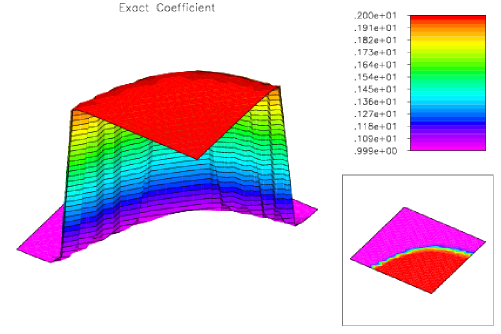
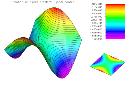
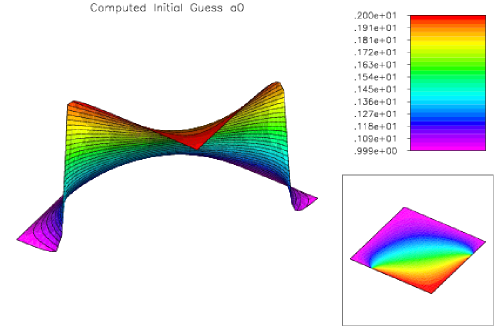
Figure 1: First experiment: setup of the problem. Top: The parameter $a^{\star}(x)$ to be identified; Center: Voltage source $U(x)$ (Dirichlet boundary condition at $\partial\Omega$ for the DtN map) and the corresponding solution $\hat{u}$ of (24); Bottom: Initial guess $a_{0}(x)$ for the iterative methods PLW, LW and SD.

$\bullet$ The parameter space is $H^{1}(\Omega)$ and the function $a^{\star}(x)(x)$ to be identified is shown in Figure 1.

$\bullet$ The fixed Dirichlet input for the DtN map (24) is the continuous function $U:\partial\Omega\to\mathbb{R}$ defined by

$$U(x,0)\ =\ U(x,1)\ :=\ \sin(\pi x)\,,\quad U(0,y)\ =\ U(1,y)\ :=\ -\sin(\pi y)$$

(in Figure 1, $U(x)$ and the corresponding solution $\hat{u}$ of (24) are plotted).

$\bullet$ The TCC constant $\eta$ in (5) is not known for this particular setup. In our computations we used the value $\eta=0.45$ which is in agreement with A2.
(Note that the convergence analysis of the PLW method requires $\eta<1$ while the nonlinear LW method requires the TCC with $\eta<0.5$ [11, Assumption (2.4)]. The above choice allows the comparison of both methods.)

$\bullet$ The “exact data” $y$ in (25) is obtained by solving the direct problem (24) using a finite element type method and adaptive mesh refinement (approx 131.000 elements). In order to avoid inverse crimes, a coarser grid (with approx 33.000 elements) was used in the finite element method implementation of the iterative methods.

$\bullet$ In the numerical experiment with noisy data, artificially generated (random) noise of 2% was added to the exact data $y$ in order to generate the noisy data $y^{\delta}$. For the verification of the stopping rule (20) we assumed exact knowledge of the noise level and chose $\tau=3$ in (19), which is in agreement with the above choice for $\eta$.

Remark 5.1 (Choosing the initial guess).

The initial guess $a_{0}(x)$ used for all iterative methods is presented in Figure 1. According to A1 – A3, $a_{0}(x)$ has to be sufficiently close to $a^{\star}(x)$ (otherwise the PLW method may not converge). With this in mind, we choose $a_{0}(x)$ as the solution of the Dirichlet boundary value problem

$$\Delta a_{0}\ =\ 0\,,\ \mbox{in }\Omega\,,\quad\quad a_{0}(x)\ =\ U(x)\,,\ \mbox{at }\partial\Omega\,.$$

This choice is an educated guess that incorporate the available a priori knowledge about the exact solution $a^{\star}(x)$, namely: $a_{0}\in H^{1}(\Omega)$ and $a_{0}(x)=a^{\star}(x)$ at $\partial\Omega_{D}$. Moreover, $a_{0}=\operatorname{arg\,min}\{\|\nabla a\|_{L^{2}(\Omega)}^{2}$ $|$ $a\in H^{1}(\Omega)$, $a_{\partial\Omega}(x)=a^{\star}_{\partial\Omega}(x)\}$.

Remark 5.2 (Computing the iterative step).

The computation of the $k$th-step of the PLW method (see (8)) requires the evaluation of $F^{\prime}(a_{k})^{*}F_{0}(a_{k})$. According to [3], for all test functions $v\in H^{1}_{0}(\Omega)$ it holds

$$\langle F^{\prime}(a_{k})^{\times}F_{0}(a_{k}),v\rangle_{L^{2}(\Omega)}\ =\ \langle F_{0}(a_{k}),F^{\prime}(a_{k})v\rangle_{L^{2}(\partial\Omega)}\ =\ \langle F_{0}(a_{k}),V\rangle_{L^{2}(\partial\Omega)}\,,$$

where $F^{\prime}(a_{k})^{\times}$ stands for the adjoint of $F^{\prime}(a_{k})$ in $L^{2}(\Omega)$, and $V\in H^{1}(\Omega)$ solves

$$-\nabla\cdot(a_{k}(x)\,\nabla V)\ =\ \nabla\cdot(v\,\nabla F(a_{k}))\,,\ \mbox{in }\Omega\,,\quad\quad V\ =\ 0\,,\ \mbox{at }\partial\Omega\,.$$

Furthermore, in [3] it is shown that for all $\psi\in L^{2}(\partial\Omega)$ and $v\in H^{1}_{0}(\Omega)$

$$\langle F^{\prime}(a_{k})^{\times}\psi,v\rangle_{L^{2}(\Omega)}\ =\ \langle\psi,V\rangle_{L^{2}(\partial\Omega)}\ =\ \langle\nabla\Psi\cdot\nabla u_{k},v\rangle_{L^{2}(\Omega)}\,,$$ (26)

where $\Psi$, $u_{k}$ $\in H^{1}(\Omega)$ solve

$$-\nabla\cdot(a_{k}(x)\,\nabla\Psi)\ =\ 0\,,\ \mbox{in }\Omega\,, \quad\quad\Psi\ =\ \psi\,,\ \mbox{at }\partial\Omega$$ (27a)

$$-\nabla\cdot(a_{k}(x)\,\nabla u_{k})\ =\ 0\,,\ \mbox{in }\Omega\,, \quad\quad u_{k}\ =\ U(x)\,,\ \mbox{at }\partial\Omega\,.$$ (27b)

respectively. An direct consequence of (26), (27) is the variational identity

$$\langle F^{\prime}(a_{k})^{\times}F_{0}(a_{k}),v\rangle_{L^{2}(\Omega)}\ =\ \langle\nabla\Psi\cdot\nabla u_{k},v\rangle_{L^{2}(\partial\Omega)}\,,\ \forall v\in H^{1}_{0}(\Omega)\,,$$

where $\Psi$ solves (27a) with $\psi=F_{0}(a_{k})$.

Notice that $\nabla\Psi\cdot\nabla u_{k}$ is the adjoint, in $L^{2}(\Omega)$, of $F^{\prime}(a_{k})$ applied to $F_{0}(a_{k})$. We need to apply to $F_{0}(a_{k})$, instead, the adjoint of $F^{\prime}(a_{k})$ in $H^{1}(\Omega)$. That is, we need to compute

$$F^{\prime}(a_{k})^{*}F_{0}(a_{k})=W_{k}\in H^{1}_{0}(\Omega)\,,$$

where $W_{k}$ is the Riesz vector satisfying  $\langle W_{k},v\rangle_{H^{1}(\Omega)}=\langle\nabla\Psi\cdot\nabla u_{k},v\rangle_{L^{2}(\Omega)}$, for all $v\in H^{1}(\Omega)$. A direct calculation yields

$$(I-\Delta)\,W_{k}\ =\ \nabla\Psi\cdot\nabla u_{k}\,,\ \mbox{in }\Omega\,,\quad\quad W_{k}\ =\ 0\,,\ \mbox{at }\partial\Omega\,.$$

Within this setting, the PLW iteration (8) becomes

$$a_{k+1}\ :=\ a_{k}\,-\,(1-\eta)\dfrac{\|F_{0}(a_{k})\|_{L^{2}(\Omega)}^{2}}{\|W_{k}\|_{H^{1}(\Omega)}^{2}}\ W_{k}\,.$$

The iterative steps of the benchmark iterations LW and SD (implemented here for the sake of comparison) are computed also using the adjoint of $F^{\prime}(\cdot)$ in $H^{1}$. Notice that a similar argumentation can be derived in the noisy data case (see (17)).

For solving the elliptic PDE’s above described, needed for the implementation of the iterative methods, we used the package PLTMG [2] compiled with GFORTRAN-4.8 in a INTEL(R) Xeon(R) CPU E5-1650 v3.

First example: Problem with exact data.
Evolution of both iteration error and residual is shown in Figure 2. The PLW method (GREEN) is compared with the LW method (BLUE) and with the SD method (RED). For comparison purposes, if one decides to stop iterating when $\|F_{0}(a_{k})\|<0.025$ is satisfied, the PLW method needs only 43 iterations, while the SD method requires 167 iterative steps and the LW method required more than 500 steps.

Second example: Problem with noisy data.
Evolution of both iteration error and residual is shown in Figure 3. The PLW method (GREEN) is compared with the LW method (BLUE) and with the SD method (RED). The stop criteria (20) is reached after 14 steps of the PLW iteration, 32 steps for the SD iteration, and 56 steps for the LW iteration.

5.4 Second experiment: The semiconductor setup

In this paragraph we consider the more realistic setup (in agreement with the semiconductor models in Subsection 5.1) with $\partial\Omega_{D}\not\subseteq\partial\Omega$, and $\Gamma_{0}\neq\emptyset$, $\partial\Omega_{N}\neq\emptyset$.

In this experiment we have: (i) The voltage profile $U\in H^{1/2}(\partial\Omega_{D})$ satisfies $U|_{\Gamma_{1}}=0$; (ii) As in the previous experiment, the identification of $a(x)$ is performed from a single measurement. To the best of our knowledge, within this setting, Assumptions A1 – A3 where not yet established for the operator $F$ in (25) and its discretizations. Therefore, although the operator $F$ is continuous [3], it is still unclear whether the analytical convergence results of the previous sections hold here.

The setup of the numerical experiments presented in this section is the following:

$\bullet$ The elements listed below are the same as in the previous experiment:

— The domain $\Omega\subset\mathbb{R}^{2}$;

— The parameter space $H^{1}(\Omega)$ and the function $a^{\star}(x)$ to be identified;

— The computation of the “exact data” $y$ in (25);

— The choice for the TCC constant $\eta$ in (5) and for $\tau$ in (19);

— The level $\delta$ of artificially introduced noise;

— The procedure to generate the noisy data $y^{\delta}$;

$\bullet$ The boundary parts mentioned in Subsection 5.1 are defined by $\partial\Omega_{D}:=\Gamma_{0}\cup\Gamma_{1}$, $\Gamma_{1}:=\{(x,1)\,;\ x\in(0,1)\}$, $\Gamma_{0}:=\{(x,0)\,;\ x\in(0,1)\}$, $\partial\Omega_{N}:=\{(0,y)\,;\ y\in(0,1)\}\cup\{(1,y)\,;\ y\in(0,1)\}$.
(in Figure 4 (a) and (b), the boundary part $\Gamma_{1}$ corresponds to the lower left edge, while $\Gamma_{0}$ is the top right edge; the origin is on the upper right corner).

$\bullet$ The fixed Dirichlet input for the DtN map (24) is the piecewise constant function $U:\partial\Omega_{D}\to\mathbb{R}$ is defined by  $U(x,0):=1$, and $U(x,1)=0$. In Figure 4 (a), $U(x)$ and the corresponding solution $\hat{u}$ of (24) are plotted.

$\bullet$ The initial condition $a_{0}(x)$ used for all iterative methods is shown in Figure 4 (b) and is given by the solution of the mixed boundary value problem

$$\Delta a_{0}(x)\ =\ 0\,,\ \mbox{in }\Omega\,,\quad\quad a_{0}(x)\ =\ U(x)\,,\ \mbox{at }\partial\Omega_{D}\,,\quad\quad\nabla a_{0}\cdot\nu\ =\ 0\,,\ \mbox{at }\partial\Omega_{N}\,,$$

analogously as in Remark 5.1.

$\bullet$ The computation of the iterative-step of the PLW method is performed analogously as in Remark 5.2, namely

$$a_{k+1}\ :=\ a_{k}\,-\,(1-\eta)\dfrac{\|F_{0}(a_{k})\|_{L^{2}(\Omega)}^{2}}{\|W_{k}\|_{H^{1}(\Omega)}^{2}}\ W_{k}\,.$$

where the Riesz vector $W_{k}\in H^{1}(\Omega)$ solves

$$(I-\Delta)\,W_{k}=\nabla\Psi\cdot\nabla u_{k},\ \mbox{in }\Omega,\quad W_{k}=0,\ \mbox{at }\partial\Omega_{D},\quad\nabla W_{k}\cdot\nu=0,\ \mbox{at }\partial\Omega_{N},$$

and $\Psi$, $u_{k}$ solve

$$-\nabla\cdot(a_{k}(x)\,\nabla\Psi)=0,\ \mbox{in }\Omega, \quad\Psi=F_{0}(a_{k}),\ \mbox{at }\partial\Omega_{\Gamma_{1}},\quad \nabla\Psi\cdot\nu=0,\ \mbox{at }\partial\Omega_{N},$$

$$\quad\Psi=0,\hskip 25.6073pt\ \mbox{at }\partial\Omega_{\Gamma_{0}},\quad$$

$$-\nabla\cdot(a_{k}(x)\,\nabla u_{k})=0,\ \mbox{in }\Omega, \quad u_{k}=U(x),\,\ \ \mbox{at }\partial\Omega_{D},\quad \nabla u_{k}\cdot\nu=0,\ \mbox{at }\partial\Omega_{N}.$$

Example: Problem with exact data.
Evolution of both iteration error and residual is shown in Figure 5. The PLW method (GREEN) is compared with the LW method (BLUE) and with the SD method (RED).

Second example: Problem with noisy data.
Evolution of both iteration error and residual is shown in Figure 6. The PLW method (GREEN) is compared with the LW method (BLUE) and with the SD method (RED). The stop criteria (20) is reached after 9 steps of the PLW iteration, 22 steps for the SD iteration, and 153 steps for the LW iteration.

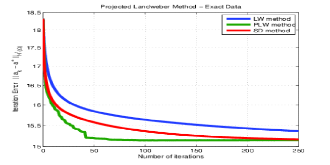
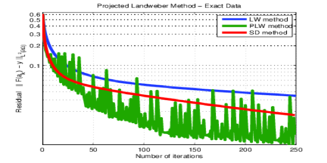
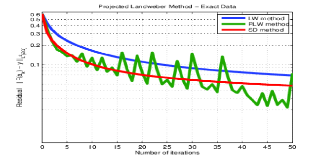
Figure 2: First experiment: example with exact data. The PLW method (GREEN) is compared with the LW method (BLUE) and with the SD method (RED); Top: Iteration error $\|a_{k}-a^{\star}\|_{H^{1}(\Omega)}$; Middle: Residual $\|F(a_{k})-y\|_{L^{2}(\partial\Omega)}$; Bottom: Residual, detail of the first 50 iterations.

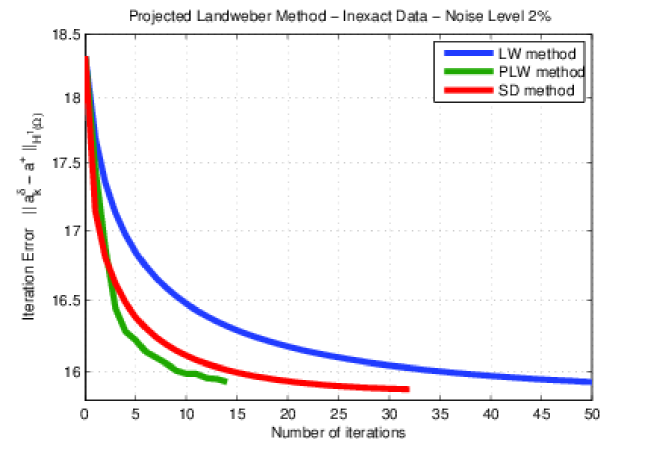
Figure 3: First experiment: example with noisy data. The PLW method (GREEN) is compared with the LW method (BLUE) and with the SD method (RED); Top: Iteration error $\|a_{k}^{\delta}-a^{\star}\|_{H^{1}(\Omega)}$; Bottom: Residual $\|F(a_{k}^{\delta})-y^{\delta}\|_{L^{2}(\partial\Omega)}$.

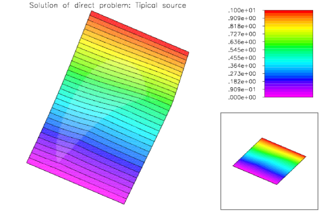
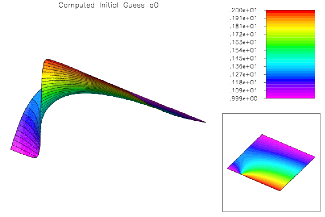
Figure 4: Second experiment: setup of the problem. Top: Voltage source $U(x)$ (Dirichlet boundary condition at $\partial\Omega_{D}$ for the DtN map) and the corresponding solution $\hat{u}$ of (24); Bottom: Initial guess $a_{0}\in H^{1}(\Omega)$ satisfying $a_{0}(x)=U(x)$ at $\partial\Omega_{D}$ and $\nabla a_{0}(x)\cdot\nu(x)=0$ at $\partial\Omega_{N}$.

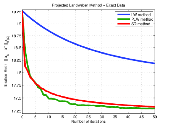
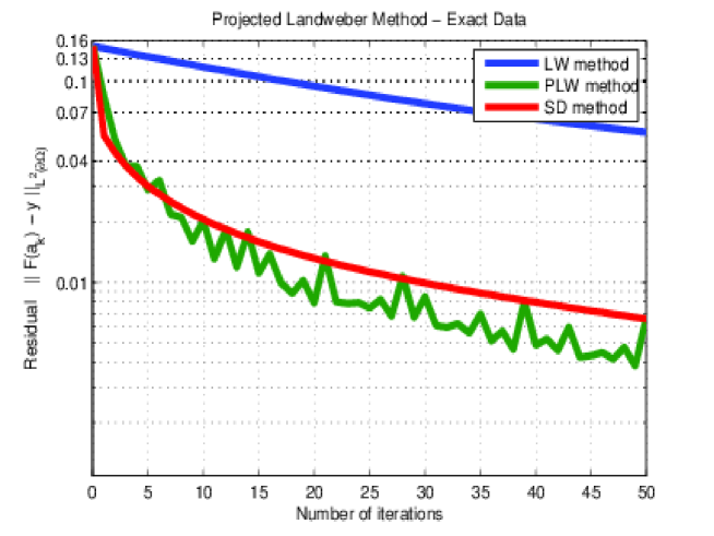
Figure 5: Second experiment: example with exact data. The PLW method (GREEN) is compared with the LW method (BLUE) and with the SD method (RED); Top: Iteration error $\|a_{k}-a^{\star}\|_{H^{1}(\Omega)}$; Bottom: Residual $\|F(a_{k})-y\|_{L^{2}(\Gamma_{1})}$.

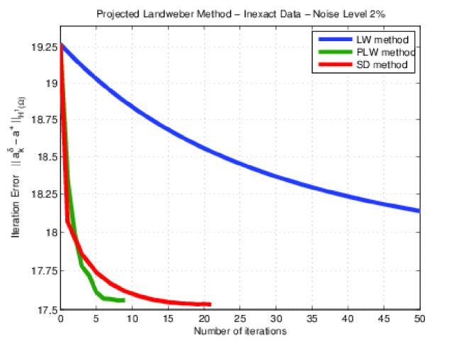
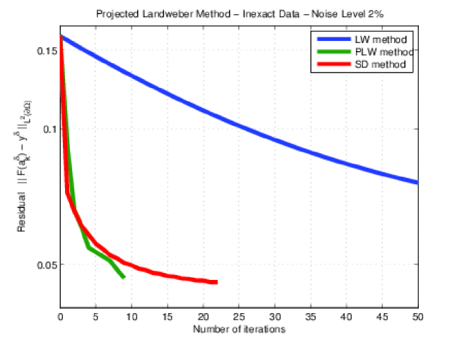
Figure 6: Second experiment: example with noisy data. The PLW method (GREEN) is compared with the LW method (BLUE) and with the SD method (RED); Top: Iteration error $\|a_{k}^{\delta}-a^{\star}\|_{H^{1}(\Omega)}$; Bottom: Residual $\|F(a_{k}^{\delta})-y^{\delta}\|_{L^{2}(\partial\Omega)}$.

6 Conclusions

In this work we use the TCC to devise a family of relaxed projection Landweber methods for solving operator equation (2). The distinctive features of this family of methods are:

• the basic method in this family (the PLW method) outperformed, in our preliminary numerical experiments, the classical Landweber method as well as the steepest descent method (with respect to both the computational cost and the number of iterations);

• the PLW method is convergent for the constant of the TCC in a range twice as large as the one required for the convergence of Landweber and other gradient type methods;

• for noisy data, the iteration of the PLW method progresses towards the solution set for residuals twice as small as the ones prescribed by the discrepancy principle for Landweber [6, Eq. (11.10)] and steepest descent [23, Eq. (2.4)] methods. This follows from the fact that the constant prescribed by the discrepance principle for our method and for Landweber/steepest-descent are, respectively

  $$\tau\ =\ \frac{1+\eta}{1-\eta}\quad\text{ and }\quad\tau\ =\ 2\frac{1+\eta}{1-2\eta};$$

• the proposed family of projection-type methods encompasses, as particular cases, the Landweber method, the steepest descent method as well as the minimal error method; thus, providing an unified framework for their convergence analysis.

In our numerical experiments, the residue in the PLW method has very strong oscillations for noisy data (Fig…) and for exact data (Fig.) Since this method iterations’ aims to reduce the iteration error, a non-monotone behavior of the residual is to be expected. In ill-posed problem error and residual are poor correlated, which may explain the large variations on the second one observed in our experiments with the PLW. Up to now it is not clear to us why this non-monotonicity happened to be oscillatory in our experiments.

Although projection type methods for solving systems of linear equations dates back to [4, 10], the use of these methods for ill-posed equations is more recent, see, e.g, [20].

A family of relaxed projection gradient-type methods for solving linear ill-posed operator equations was proposed in [17]. In this work we extended to the non-linear case, under the TCC, the analysis of [17].

References

- [1] A. Bakushinsky and M. Kokurin. Iterative Methods for Approximate Solution of Inverse Problems, volume 577 of Mathematics and Its Applications. Springer, Dordrecht, 2004.
- [2] R. E. Bank. PLTMG: a software package for solving elliptic partial differential equations, volume 15 of Frontiers in Applied Mathematics. Society for Industrial and Applied Mathematics (SIAM), Philadelphia, PA, 1994. Users’ guide 7.0.
- [3] M. Burger, H. W. Engl, A. Leitão, and P. Markowich. On inverse problems for semiconductor equations. Milan J. Math., 72:273–313, 2004.
- [4] G. Cimmino. Calcolo approssimato per le soluzioni dei sistemi di equazioni lineari. La Ricerca Scientifica, XVI(9):326–333, 1938.
- [5] B. Eicke. Iteration methods for convexly constrained ill-posed problems in Hilbert space. Numer. Punct. Anal. Optim., 13:413–429, 1992.
- [6] H. Engl, M. Hanke, and A. Neubauer. Regularization of Inverse Problems. Kluwer Academic Publishers, Dordrecht, 1996.
- [7] M. Hanke, A. Neubauer, and O. Scherzer. A convergence analysis of Landweber iteration for nonlinear ill-posed problems. Numer. Math., 72:21–37, 1995.
- [8] G. T. Herman. A relaxation method for reconstructing objects from noisy X-rays. Math. Programming, 8:1–19, 1975.
- [9] G. T. Herman. Image reconstruction from projections. Academic Press, Inc. [Harcourt Brace Jovanovich, Publishers], New York-London, 1980. The fundamentals of computerized tomography, Computer Science and Applied Mathematics.
- [10] S. Kaczmarz. Angenäherte auflösung von systemen linearer gleichungen. Bulletin International de l’Académie Polonaise des Sciences et des Lettres, 35:355–357, 1937.
- [11] B. Kaltenbacher, A. Neubauer, and O. Scherzer. Iterative regularization methods for nonlinear ill-posed problems, volume 6 of Radon Series on Computational and Applied Mathematics. Walter de Gruyter GmbH & Co. KG, Berlin, 2008.
- [12] L. Landweber. An iteration formula for Fredholm integral equations of the first kind. Amer. J. Math., 73:615–624, 1951.
- [13] A. Lechleiter and A. Rieder. Newton regularizations for impedance tomography: convergence by local injectivity. Inverse Problems, 24(6):065009, 18, 2008.
- [14] A. Leitão. Semiconductors and Dirichlet-to-Neumann maps. Comput. Appl. Math., 25(2-3):187–203, 2006.
- [15] A. Leitao, P. Markowich, and J. Zubelli. Inverse Problems for Semiconductors: Models and Methods, chapter in Transport Phenomena and Kinetic Theory: Applications to Gases, Semiconductors, Photons, and Biological Systems, Ed. C.Cercignani and E.Gabetta. Birkhäuser, Boston, 2006.
- [16] A. Leitao, P. Markowich, and J. Zubelli. On inverse dopping profile problems for the stationary voltage-current map. Inv.Probl., 22:1071–1088, 2006.
- [17] S. McCormick and G. Rodrigue. A uniform approach to gradient methods for linear operator equations. J. of Math. Anal. and Applications, 49(2):275–285, 1975.
- [18] V. Morozov. Regularization Methods for Ill–Posed Problems. CRC Press, Boca Raton, 1993.
- [19] F. Natterer. Regularisierung schlecht gestellter Probleme durch Projektionsverfahren. Numer. Math., 28(3):329–341, 1977.
- [20] F. Natterer. The mathematics of computerized tomography. B. G. Teubner, Stuttgart; John Wiley & Sons, Ltd., Chichester, 1986.
- [21] A. Neubauer and O. Scherzer. A convergence rate result for a steepest descent method and a minimal error method for the solution of nonlinear ill-posed problems. J. for Analysis ans its Applications, 14:369–377, 1995.
- [22] O. Scherzer. Convergence rates of iterated Tikhonov regularized solutions of nonlinear ill-posed problems. Numer. Math., 66(2):259–279, 1993.
- [23] O. Scherzer. A convergence analysis of a method of steepest descent and a two-step algorithm for nonlinear ill-posed problems. Numer. Funct. Anal. Optim., 17(1-2):197–214, 1996.
- [24] T. Seidman and C. Vogel. Well posedness and convergence of some regularisation methods for non–linear ill posed problems. Inverse Probl., 5:227–238, 1989.
- [25] A. Tikhonov. Regularization of incorrectly posed problems. Soviet Math. Dokl., 4:1624–1627, 1963.
- [26] A. Tikhonov and V. Arsenin. Solutions of Ill-Posed Problems. John Wiley & Sons, Washington, D.C., 1977. Translation editor: Fritz John.
- [27] V. V. Vasin and I. I. Eremin. Operators and iterative processes of Fejér type. Inverse and Ill-posed Problems Series. Walter de Gruyter GmbH & Co. KG, Berlin, 2009. Theory and applications.