A search for X-ray absorbed sources in the 3XMM catalogue, using photometric redshifts and Bayesian spectral fits

Since its launch in 1999, the XMM-Newton mission has compiled the largest catalogue of serendipitous X-ray sources, with the 3XMM being the third version of this catalogue. This is because of the combination of a large effective area (5000 $\rm cm^{2}$ at 1 keV) and a wide field of view (30 arcmin). The 3XMM-DR6 catalogue contains about 470 000 unique X-ray sources over an area of 982 $\rm deg^{2}$. A significant fraction of these (100 178 sources) have reliable optical, near/mid-IR counterparts in the SDSS, PANSTARRS, VIDEO, UKIDSS and WISE surveys. In a previous paper we have presented photometric redshifts for these sources using the TPZ machine learning algorithm. About one fourth of these (22 677) have adequate photon statistics so that a reliable X-ray spectrum can be extracted. Obviously, owing to both the X-ray counts selection and the optical counterpart constraint, the sample above is biased towards the bright sources. Here, we present XMMFITCAT-Z: a spectral fit catalogue for these sources using the Bayesian X-ray Analysis (BXA) technique. As a science demonstration of the potential of the present catalogue, we comment on the optical and mid-IR colours of the 765 X-ray absorbed sources with $N_{\mathrm{H}}>10^{22}\,\mathrm{cm}^{-2}$. We show that a considerable fraction of X-ray selected AGN would not be classified as AGN following the mid-IR W1–W2 vs. W2 selection criterion. These are AGN with lower luminosities, where the contribution of the host galaxy to the MIR emission is non-negligible. Only one third of obscured AGN in X-rays present red colours or r–W2 ¿ 6. Then it appears that the r–W2 criterion, often used in the literature for the selection of obscured AGN, produces very different X-ray absorbed AGN samples compared to the standard X-ray selection criteria.

1 Introduction

The XMM-Newton mission (Jansen et al., 2001) launched in 1999 is the European Space Agency’s (ESA) second cornerstone mission. It carries onboard three telescopes with the largest effective area in a X-ray telescope so far (combined 5000 cm² at 1 keV). These telescopes focus the light on the European Photon Imaging Camera (EPIC) CCD cameras. Owing to its large field-of-view ($\sim 30$ arcmin diameter), it can detect a large number of serendipitous sources in each observation. The Survey Science Centre (SSC), a consortium of ten European Institutes, was formed and is responsible for producing the catalogues of the serendipitous sources detected. The third version of this catalogue (3XMM) has been published and is described in detail in Rosen et al. (2016). The 3XMM covers about 1000 square degrees and contains about half a million unique sources. This is the largest catalogue of X-ray sources ever produced. Their median flux of the sources is $\sim 2.4\times 10^{-14}\,\mathrm{erg\,cm^{-2}\,s^{-1}}$ in the total 0.2–12 keV band.

The large sky area of the 3XMM offers the opportunity of identify rare objects that are harder to find in deeper surveys with much smaller sky areas, like high luminosity active galactic nuclei (AGN). Moreover, the sensitivity and energy range of the 3XMM allows the detection of X-ray absorbed AGN, which are elusive in shallower and/or softer surveys. In addition, the SSC provides spectral products for a large number of 3XMM sources, allowing a systematic study of the spectral properties of the 3XMM.

The goal of this work was the construction of a clean, reliable sample of X-ray absorbed AGN, after a robust, systematic analysis of their X-ray spectra included in the 3XMM. Given the size of the available data (more than 170 000 spectra in the sixth version of the catalogue, 3XMM-DR6), the use of automated spectral modelling techniques is mandatory. The XMM-Newton spectral-FIT CATalogue (XMMFITCAT; Corral et al., 2015) was a previous effort in this direction. This catalogue offers spectral fits for a large fraction of 3XMM sources having spectral data and it has been used to identify X-ray absorbed sources (Corral et al., 2014). However, due to the lack of redshift information for the majority of 3XMM sources, it was not possible to provide physical, reliable estimations for the X-ray absorption (i.e. Hydrogen column density) or other spectral parameters and derived quantities (e.g. temperature of plasmas or luminosities).

Obtaining spectroscopic redshifts for the bulk of the 3XMM catalogue would be extremely costly in observational terms. Therefore, using photometric redshifts is the only feasible technique to obtain distance information for such a large number of sources. The XMM-Newton Photo-Z CATalogue (XMMPZCAT) offers photometric redshifts for a large fraction of 3XMM sources: In the framework of the ESA Prodex project we derived photometric redshifts for 100 178 X-ray sources, about 50% of the total number of 3XMM sources (205 380) in the XMM-Newton fields selected to build XMMPZCAT (4208 out of 9159). The photometric redshifts were derived using a machine learning algorithm, Trees for Photo-Z (TPZ; Carrasco Kind & Brunner, 2013). The optical photometry used for the derivation of photometric redshifts included the SDSS survey and the PANSTARS survey, with ancillary data in near- (2MASS, UKIDSS, VISTA) and mid-IR (All-WISE survey) bands. See Ruiz et al. (2018) for a complete description of this catalogue.

In this work we combine the results of XMMPZCAT with the automated spectral fitting approach of XMMFITCAT in order to estimate X-ray models and the corresponding spectral properties for 30 816 3XMM detections. These results are collected in the XMM-Newton spectral-fit z catalogue (XMMFITCAT-Z).

As a demonstration of the scientific potential of XMMFITCAT-Z, we searched for sources showing spectral features of X-ray absorbed AGN. We found 1421 spectra with signs of X-ray absorption ($\sim 5\%$ of the total catalogue), corresponding to 1037 unique sources. After further examination of their X-ray properties, we selected in our final sample 977 detections, corresponding to 765 unique sources, showing highly reliable absorption features and redshift estimations.

The structure of the paper is as follows: in Sect. 2 we describe the XMMFITCAT-Z, including the data and techniques to build the catalogue. Section 3 explains our methodology to identify X-ray absorption and the final atlas of X-ray absorbed AGN. In Sect. 4 we discuss our results, while Sect. 5 summarizes the main conclusions of this work.

2 XMMFITCAT-Z: A catalogue of automatic X-ray spectral fitting

In this work we present the XMM-Newton spectral-fit z catalogue (XMMFITCAT-Z): using the pipeline spectral products from the 3XMM catalogue (see Sect. 2.1.1) and the redshifts we derived in XMMPZCAT (see Sect. 2.1.2), we built a catalogue of X-ray spectral fits, similar to XMMFITCAT (Corral et al., 2015) but now including the distance information in an automated spectral fitting process. This allows the estimation of important physical parameters from the X-ray spectra like rest-frame column densities, temperature of emitting plasma, intrinsic fluxes and luminosities.

XMMFITCAT-Z contains spectral-fitting results for 30 816 source detections, corresponding to 22 677 unique sources. The version of the catalogue used to construct the current catalogue is 3XMM-DR6. Not all detections with extracted spectra are included in this database. To ensure the reliability of the spectral-fitting results, a constrain has been imposed to the number of counts collected in the X-ray spectra (Sect. 2.1.1) and as result, some detections are rejected in the automated spectral-fit pipeline. Moreover, only detections with redshifts in XMMPZCAT have been included (Sect. 2.1.2). We offer two main products to the final user: A single FITS table containing the most useful data from XMMFITCAT-Z, and a relational database with all information.

The main results of the XMMFITCAT-Z database are summarized in a table in FITS format. It contains one row for each detection included in the database, and 157 columns containing information about the source detection and the spectral-fitting results. The first 14 columns contain information about the source and observation, including redshift information, whereas the remaining 143 columns contain, for each model applied, model spectral-fit flags, parameter values and errors, fluxes, luminosities and five columns to describe the goodness of the fit. See Appendix A for a full description of all the columns included in the table.

We also offer the full XMMFITCAT-Z database as a file in SQLite format that can be downloaded by the final user. The SQLite version contains significantly more information than the FITS table and allows performing advanced queries using SQL language. It is composed of 11 tables that store all the information about the detections, the spectra used in the automatic fitting and the results: fit statistics, best-fit parameters, fluxes and luminosities. A complete description of all tables and parameters is available in the XMMFITCAT-Z web-site.

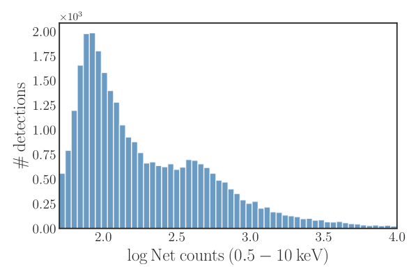
Figure 1: Distribution of net counts (background subtracted spectral counts) per observation used in the automated spectral fits. Observations with more than 10,000 counts are not included in this plot.

2.1 Data

2.1.1 XMM-Newton data

3XMM-DR6 is the third generation catalogue of serendipitous X-ray sources from the ESA’s XMM-Newton observatory, and has been created by the XMM-Newton SSC on behalf of ESA. The 3XMM-DR6 catalogue contains X-ray photometric information for 678 680 X-ray detections.

Each XMM-Newton observation considered for the construction of the 3XMM goes through the SSC source detection pipeline independently, obtaining a list of detections for each observation. Since some of these observations correspond to overlapping sky areas, a fraction of these detections can be associated to the same physical object (i.e. unique source). The 3XMM catalogue groups as a single entry these detections that are assumed to be the same physical source. When taking this into account, the 678 680 detections included in the 3XMM-DR6 are reduced to 468 440 unique sources.

As part of the catalogue production, spectra and time series are also extracted in the case of detections with more than 100 counts collected in the EPIC camera. This corresponds to 149 998 detections, and 102 157 unique sources. The spectral data from the 3XMM-DR6 catalogue were screened before applying our automated spectral-fitting pipeline so that spectral fits are only performed if the data fulfil the following criteria:

• Only spectra corresponding to a single instrument and observation with more than 50 net counts (i.e. background subtracted) in the 0.5–10 keV band are used in the spectral fits. This means that some detections with more than 100 EPIC counts in the total band, but less than 50 counts in each different EPIC instrument (EPIC-pn, EPIC-MOS1, or EPIC-MOS2), are excluded from the automated fits, and therefore, they are not included in the spectral-fit database.

• Complex models (see Sect. 2.3), are only applied if the number of EPIC counts is larger than 500 net counts in the total 0.5–10 keV band.

As a result of the application of these criteria, the spectral-fit database contains results corresponding to the simple models for 30 816 source detections, corresponding to 22 677 unique sources (see Table LABEL:tab:sourcenumbers). Spectral-fitting results for complex models are available for 4797 detections. The distribution of spectral counts per observation used during the automated fits is plotted in Fig. 1. Observations with more than 10 000 counts, 2% of the 30 816 detections, are excluded of this plot for clarity.

2.1.2 Photometric redshifts

The XMM-Newton Photo-Z Catalogue (XMMPZCAT, Ruiz et al., 2018) contains photometric redshifts for 100 178 X-ray sources in the 3XMM, that is about 50% of the X-ray sources within the selected XMM-Newton observations to build the catalogue. It contains sources outside the Galactic plane (—b—¿20 deg) with highly reliable optical counterparts in the SDSS-DR13 or Pan-STARRS-DR1 catalogues.

This catalogue was produced through a machine learning algorithm, MLZ-TPZ (Carrasco Kind & Brunner, 2013), by using optical (SDSS and Pan-STARRS) and (if available) near- (2MASS, UKIDSS, VISTA) and/or mid-IR (All-WISE) photometry , to derive photometric redshifts. The version of the catalogue used to construct the current XMMPZCAT is 3XMM-DR6. Optical and IR data were obtained from multiwavelength cross-matched catalogues using tools and results from the ARCHES project (Motch et al., 2017; Pineau et al., 2017).

XMMPZCAT also includes spectroscopic redshifts for 12 693 sources, obtained either from the SDSS or other spectroscopic surveys used for training the machine learning algorithm, like XXL (Menzel et al., 2016), XMS (Barcons et al., 2007) or XBS (Della Ceca et al., 2004). See Mountrichas et al. (2017a); Ruiz et al. (2018) for a detailed description of these surveys. If available, we used these spectroscopic redshifts for the X-ray spectral fits.

Table 1: Number of sources

Sample	Detections	Unique	WISE
		sources
XMMPZCAT	-	100178	61998
XMMFITCAT-Z (total)	30816	22677	17133
X-ray non-AGN	1881	1433	1181
X-ray AGN unabsorbed	17158	12686	10116
X-ray AGN absorbed	977	765	668

2.2 Bayesian X-ray Analysis

We used the fitting and modelling software Sherpa 4.9.1 (Freeman et al., 2001) to perform the automated spectral fits. We followed the Bayesian technique proposed in Buchner et al. (2014) using the Bayesian X-ray Analysis (BXA) software, which connects the nested sampling algorithm MultiNest (Feroz et al., 2009) with Sherpa.

By using BXA we can incorporate the whole probability distribution for each photometric redshift as a prior in the model fitting. Moreover, a nested sampling algorithm like MultiNest allows for a full exploration of the parameter space, avoiding finding only solutions for local minima, a common problem that arise when using standard minimization techniques like e.g. the Levenberg-Marquardt algorithm.

In the BXA framework, the use of Cash statistics (Cash, 1979) is mandatory. We used the wstat implementation in Sherpa, which allows using background datasets as background models. wstat is used for modelling Poisson data with Poisson background when no physically motivated background model is available. It assumes a background model with as many parameters as bins in the background spectrum. Under certain assumptions, there is an analytical solution for calculating the values of these parameters (see e.g. Appendix B of the Xspec User’s Guide). For using the wstat statistics, the grouped spectra from the 3XMM-DR6 catalogue were ungrouped, and then grouped to 1 count per bin.

All available instruments and exposures for a single observation of a source were fitted together, using spectral data within the 0.5–10 keV band. All model parameters for different instruments are tied together except for a relative normalization, which accounts for the differences in flux calibration between instruments.

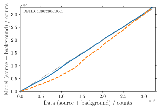
Figure 2: Q-Q plots for a 3XMM spectrum (EPIC-pn) fitted with a an absorbed power-law (blue, solid line) and an absorbed thermal model (orange, dashed line).

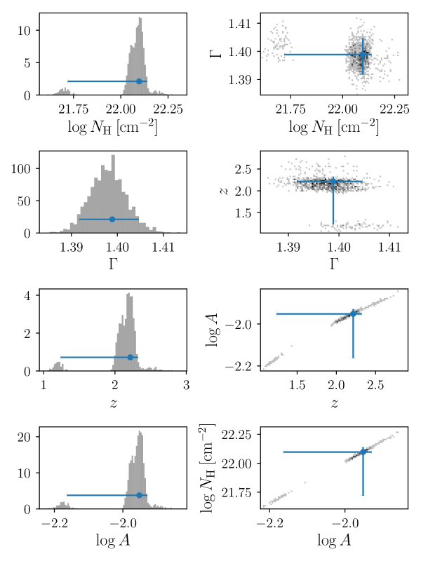
Figure 3: Posterior distributions for a 3XMM detection (DETID 106909002010001) fitted with an absorbed power-law. Left column: marginal distributions for Hydrogen column density, photon index, redshift and power-law normalization. Right column: two-parameters conditional distributions. Blue circles with error bars show the best-fit value of the parameters and the corresponding 90% credible intervals.

2.3 Models and priors

Most sources included in XMMPZCAT are extragalactic and hence the population is dominated by AGN. Given this fact, we have reduced the number of spectral models with respect to XMMFITCAT. They are phenomenological models selected to reproduced the spectral emission of AGN. We also included a simple thermal model to deal with the X-ray emission of stars (about ten percent of XMMPZCAT sources) and other hot plasmas (e.g. intra-cluster medium emission).

There are four different models, two simple and two more complex models, as follows:

• Simple models:

  • Absorbed power-law model (“wapo”, XSPEC: zwabs*pow): Variable parameters are the Hydrogen column density of the absorber, the power-law photon index, and the power-law normalization.

  • Absorbed thermal model (“wamekal”, XSPEC: zwabs*mekal): Variable parameters are the Hydrogen column density of the absorber, the plasma temperature of the thermal component, and the normalization of the thermal component.

• Complex models:

  • Absorbed thermal plus power-law model (“wamekalpo”, XSPEC: zwabs*(mekal + zwabs*pow)): Variable parameters are the Hydrogen column density of both absorbers, the plasma temperature, the photon index, and the normalization of the power-law and thermal components.

  • Absorbed double power-law model (“wapopo”, XSPEC: zwabs*(pow + zwabs*pow)): Variable parameters are the Hydrogen column density of both absorbers, the photon indices of both power-law components, and the corresponding normalizations.

All models include an additional absorption component, wabs, to take into account the Galactic absorption, with the Hydrogen column density fixed to the value in the direction of the source from the Leiden/Argentine/Bonn (LAB) Survey of Galactic HI (Kalberla et al., 2005).

In the BXA framework we employed for the spectral fitting, a probability prior should be assigned to each free parameter in the model. These are the priors we selected:

• Hydrogen column density: Jeffreys prior (i.e. a uniform prior in the logarithmic space) with limits $10^{20}-10^{25}\leavevmode\nobreak\ \mathrm{cm^{-2}}$.

• Power-law photon index: Gaussian prior with mean 1.9 and standard deviation 0.15. It corresponds to the photon index distribution for the AGN population as described in Nandra & Pounds (1994).

• Thermal plasma temperature: uniform prior with limits 0.08–20 keV.

• Redshift: for sources with known spectroscopic redshift, this is included as a fixed parameter in the models. When only a photometric redshift is available, the redshift is treated as a free parameter using the photo-z probability density distribution calculated in XMMPZCAT as the prior.

• Normalization: Jeffreys prior with limits $10^{-30}-1$.

• Relative normalization constants: Jeffreys prior with limits 0.01 – 100.

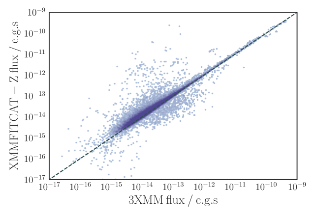
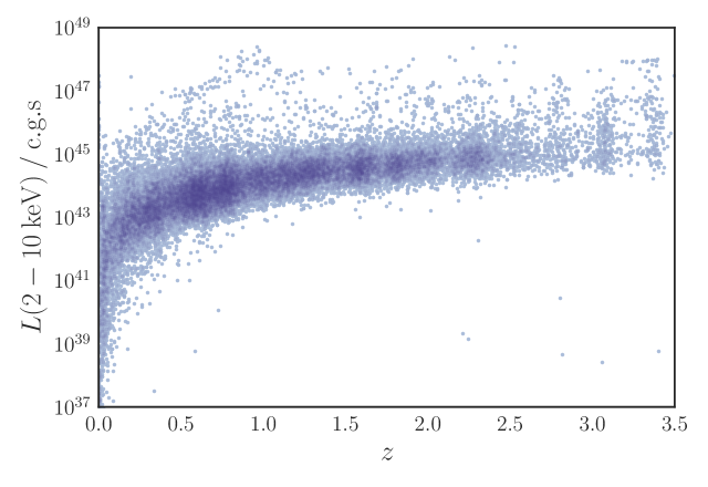
Figure 4: Left: Soft fluxes (in c.g.s. units) computed from the automated fits (P_MODEL) against fluxes in the 3XMM-DR6 catalogue. Right: Hard luminosity versus redshift (in c.g.s. units) computed from the automated fits (P_MODEL). Darker colors show a higher density of points.

2.4 Goodness of fit

Cash maximum likelihood statistics lacks a direct estimate of goodness of fit (GoF). We followed the method proposed in Buchner et al. (2014) and we used quantile-quantile (Q-Q) plots to obtain an estimate of the GoF of our spectral fits.

A Q-Q plot compares the cumulative counts of the data (source + background) with the predicted counts (source + background) of the model (see Fig. 2). These plots gives a quick visual idea of how well the model can reproduce the data. For a quantitative estimate of the GoF we calculated the Kolmogorov-Smirnov (KS) statistic between the two cumulative distributions, and the corresponding p-value. A low KS (or a high p-value) means that the data is well reproduced by the model.

We note however that in this case the p-values for the KS statistic cannot be calculated the usual way. The cumulative distribution of the model depends on the parameters that were estimated from the data distribution, therefore the condition of independence between the two compared distributions does not hold, and hence p-values estimated using the KS probability distribution are grossly incorrect. Nevertheless, through a permutation test we can get an estimate of the p-value. For each source, we did 1000 resamplings, randomly splitting the original data+model sample in two equal-size subsamples, and estimate the corresponding KS statistic. Our estimated p-values are the ratio of resamplings that have statistics larger than the statistic of the original samples.

Any model showing a KS p-value ¡ 0.01 is considered as an acceptable fit. If we found at least one acceptable fit for a given data set, the A_FIT parameter is set to True. The XBA’s MultiNest algorithm also estimates the evidence for each model ($\log\mathrm{Z}$). The model with the highest evidence (lowest $\log\mathrm{Z}$) is selected as the preferred model (P_MODEL parameter). A preferred model is always included, even in the case that it is not an acceptable fit, showing a KS p-value above 0.01. We also list the remaining models (A_MODELS parameter) with relative evidence lower than 30, with respect to the preferred model, i.e. “very strong evidence” accordingly to the scale of Jeffreys (1961) (see also Robert et al., 2009; Buchner et al., 2014). Assuming that all models are a priori equally probable, there is no statistical reason to rule out any of the models in the set formed by P_MODEL and A_MODELS. Without additional information favouring some model, if the fit is acceptable, the simplest model should be selected as the best-fit model.

We find that 28 887 detections, 94% of the XMMFITCAT-Z detections, have an acceptable fit. Specifically, 22 427 detections (73%) have a single absorbed power-law (“wapo”) as its preferred model, and 27 659 detections (90%) have this model either as preferred or in the accepted models.

2.5 Parameter and error estimation

The MultiNest algorithm implemented in BXA gives the marginalized posterior probability distribution for all free parameters in the fitted model. We used these distributions to estimate the best-fit parameters and the corresponding errors. The best-fit values correspond to the mode (the most probable value) of the posterior distribution, estimated using a half-sample algorithm (Robertson & Cryer, 1974). Errors were estimated using the posterior distributions to calculate a 90% credible interval around the mode.

Figure 3 shows an example of the marginal and conditional (for two parameters) posterior distributions for a source fitted using an absorbed power-law. This example shows how the structure of the original photo-z probability distribution is preserved.

2.6 X-ray fluxes and luminosities

The posterior probability distribution of the free parameters was propagated to estimate the flux and errors for each model. This method preserves the structure of the uncertainty (degeneracies, multimodal structure, etc.). Reported fluxes and luminosities in the catalogue correspond to the mode of the posterior distribution, with errors estimated as 90% credible intervals. These are EPIC fluxes, meaning that, in the case of multiple instrument spectra for a single observation, the reported flux is the average of the different fluxes for each instrument and exposure.

For sources with spectroscopic redshifts, luminosities were estimated using the intrinsic fluxes and the luminosity distance corresponding to that redshift. For sources with photometric redshifts, $z$ is a free parameter and hence is propagated with the posterior distribution to estimate the corresponding luminosity distance in each case. We assumed a $\Lambda$CDM cosmology with $H_{0}=67.7,\Omega_{m}=0.307$ (Planck Collaboration et al., 2016).

We estimated fluxes and luminosities in the soft (0.5–2 keV) and hard (2–10 keV) bands. For observed fluxes these bands correspond to the observer frame. For intrinsic fluxes and luminosities they correspond to the source’s rest frame.

EPIC soft fluxes obtained from the spectral fits (using results for P_MODEL, see Appendix A) are plotted against those from the 3XMM-DR6 catalogue (EP_2_FLUX + EP_3_FLUX) in the left panel of Fig. 4, and the hard X-ray luminosity against redshift in the right panel. Fluxes from the automated fits and from the 3XMM-DR6 are consistent within errors for $\sim 70$% of the detections. The conversion from count rates to fluxes in the 3XMM assumes a simple power-law model with photon index of 1.7. Hence, we can expect that XMMFITCAT-Z sources with different spectral shapes will show larger discrepancies in flux. That is indeed the case: significant differences between flux values are more frequent among sources displaying a soft spectrum, that is, sources that are best-fitted by a power-law with a steep photon index, or by a thermal model. More than 80% of the non-matching fluxes correspond to any of these cases.

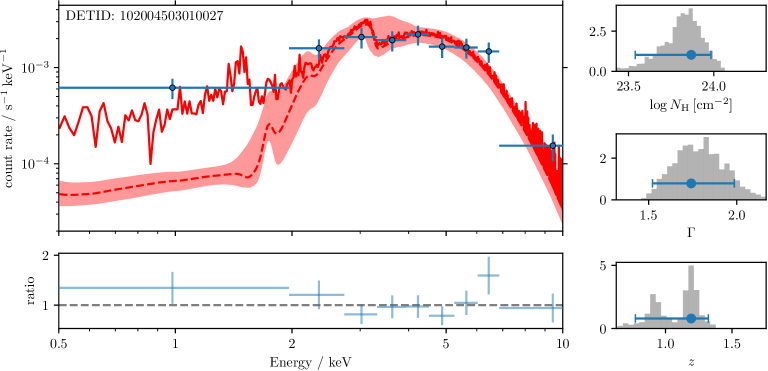
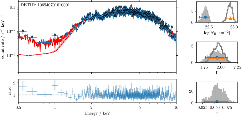
Figure 5: XMM-Newton spectra (EPIC-pn) of two X-ray absorbed AGN identified through our selection criteria. For improving visualization, spectral data (blue circles) have been grouped to obtain a signal-to-noise ratio per bin of at least five. Solid red lines: background plus model; dashed, red lines: model; red areas: $2\sigma$ model uncertainty. Panels in the lower part of the plots show the ratio between the observed and the model-predicted count rate. Histograms on the right column show the posterior probability distribution of the model parameters, the corresponding best-fit values (mode) and their 90% credible intervals. Solid, grey histograms and blue circles correspond to the outer absorber and power-law. Open histograms and orange triangles correspond to the inner model components. Top: detection best fitted with a single absorbed power-law (“wapo” model). Bottom: detection best fitted using a double power-law with two absorbers (“wapopo” model).

3 Search of X-ray absorbed sources

The basic mechanism that explains the panchromatic emission of an AGN is the accretion of gas into the central supermassive black hole of the host galaxy. The high temperatures in the inner-most regions of the accretion disk ionize the surrounding gas, creating a “hot corona” of energetic electrons. Optical and UV photons interact, through inverse Compton scattering, with the electrons in the corona, causing the characteristic X-ray emission of AGN (Haardt & Maraschi, 1991; Haardt et al., 1994).

This primary emission can be then reprocessed through other physical processes: absorption due to ionized/warm/cold material (Turner & Miller, 2009); reflection by the material in the accretion disk or by farther neutral gas (Fabian, 2006; Turner & Miller, 2009); scattering by an absorbing medium (Netzer et al., 1998); or fluorescent emission of ionized iron (Mushotzky et al., 1995; Fabian et al., 2000).

The combination of these processes can produce a quite complex X-ray spectrum in the observing spectral range of XMM-Newton ($\sim 0.2-12$ keV). However, this complexity is reasonably well captured by the phenomenological models we presented in Section 2.3: the X-ray primary emission can be modelled by a power-law with photon index $\sim 1.9$; Compton Thin neutral absorbers ($10^{22}<N_{\mathrm{H}}<10^{24}$ cm^-2) are modelled by the different absorption components included in our models; Partial absorption can be mimicked through double power-law models; Compton Thick absorption ($N_{\mathrm{H}}>10^{24}$ cm^-2), where all primary emission is suppressed below 10 keV, can be also roughly approximated by a double power-law (see below); and reflection effects are roughly modelled through power-laws or thermal emission components (“wapopo” or “wamekalpo” model). By using these simple models we found acceptable fits for 28 887 out of 30 816 (94%) X-ray spectra included in XMMFITCAT-Z.

Our first goal was to identify AGN in XMMFITCAT-Z showing spectral features of X-ray absorption. Although there exist low-luminosity AGN (see e.g. Ho, 1999; Panessa et al., 2007), any persistent astronomical source with an intrinsic (i.e. absorption corrected) 2–10 keV luminosity above $10^{42}\leavevmode\nobreak\ \mathrm{erg\,s^{-1}}$ can be associated to an AGN, no other known mechanism can produced such luminosity.

Compton Thin absorbed sources can be identify by a significant absorption component with $N_{\mathrm{H}}\gtrsim 10^{22}$ cm^-2. Compton Thick sources are harder to identify within the XMM-Newton spectral range since, as we stated above, all primary emission is suppressed below rest-frame 10 keV. Only the X-ray emission scattered by the absorbing medium is observable in this range. This emission show a flatter spectral shape with a prominent iron K_α emission line (equivalent width above 500 eV). We must note that the models used in XMMFITCAT-Z did not include iron emission lines, and hence Compton Thick sources only detectable by this spectral feature could be missed in our final sample of X-ray absorbed AGN.

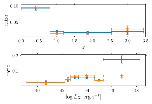
Figure 6: Ratio between X-ray absorbed and unabsorbed AGN identified in XMMFITCAT-Z for different redshift (top) and luminosity (bottom) ranges. Blue circles correspond to ratios estimated using all X-ray absorbed AGN; the ratios shown as orange stars are estimated using only absorbed AGN with a reliable best-fit model (see Sect. 4).

In summary, our selection criteria to identify X-ray absorbed AGN were:

• We first selected sources with a single absorbed power-law (“wapo”) as an accepted model (P_MODEL or in A_MODELS, and A_FIT true). Those sources showing $N_{\mathrm{H}}>10^{22}\leavevmode\nobreak\ \mathrm{cm^{-2}}$ or $\Gamma<1.4$, with 90% confidence, are classified as absorbed.

• Among those sources without “wapo” as an accepted model, we select those with a double power-law with two absorbers (“wapopo”) as an accepted model. Compton Thin sources can be identified as those showing $N_{\mathrm{H}}>10^{22}\leavevmode\nobreak\ \mathrm{cm^{-2}}$ in the inner absorber (logNH2). This model also allows for a crude approximation of the spectrum of Compton Thick objects: those showing a high obscuration in the inner absorber ($N_{\mathrm{H}}>10^{23}\leavevmode\nobreak\ \mathrm{cm^{-2}}$) and $\Gamma<1.4$ in the outer power-law (PhoIndex2).

• Finally, among those sources classified as absorbed, we selected only those showing an intrinsic 2–10 keV luminosity consistent with being greater than $10^{42}\leavevmode\nobreak\ \mathrm{erg\,s^{-1}}$ (i.e. upper error bars are above $10^{42}$).

Applying these selection criteria we found 1421 spectra with signs of X-ray absorption ($\sim 5\%$ of the total catalogue), corresponding to 1037 unique sources (out of 22 677 unique sources in the total catalogue); 1385 out of 1421 show $N_{\mathrm{H}}>10^{22}\leavevmode\nobreak\ \mathrm{cm^{-2}}$ and 38 show a flat spectrum with $\Gamma<1.4$. Two of them show both high $N_{\mathrm{H}}$ and a flat emission.

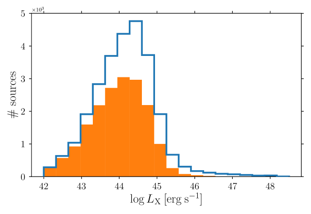
Figure 7: X-ray luminosity distribution for XMMFITCAT-Z sources classified as AGN. The solid blue line shows the whole sample without any additional filtering. The solid orange histogram includes only AGN with a reliable best-fit model (see Sect. 4).

Figure 5 show two examples of 3XMM detections included in XMMFITCAT-Z and classified as absorbed AGN following these criteria. The plots show their EPIC-pn spectra, including the best-fit model, and the corresponding best-fit parameters and their probability distributions.

To build our final selection of X-ray absorbed AGN we examined further the X-ray properties of XMMFITCAT-Z AGN (see Sect. 4). We found that our X-ray modelling for a significant fraction of sources overestimates their X-ray luminosity. This was caused by either a wrong estimation of their photometric redshifts or due to modelling artifacts introduced when using a double power-law model (“wapopo”). As we explain in Sect. 4 below, after applying an additional filtering for selecting objects with more reliable redshifts and X-ray modelling, our atlas of X-ray absorbed AGN contains 977 detections, corresponding to 765 unique sources. We provide this sample as a FITS table.

4 Discussion

In Fig. 6 we present the ratio of absorbed to unabsorbed AGN as a function of redshift (top panel) and X-ray luminosity (lower panel). Redshift and luminosity bins were estimated using the Bayesian Block Algorithm (Scargle et al., 2013). This algorithm uses a fitness function calculated on the actual data for estimating an optimal binning. It allows varying bin sizes for a better reproduction of the underlying distribution. Blue circles show the results applying the absorption criteria we presented in Sect. 5 based solely in the X-ray spectral fits.

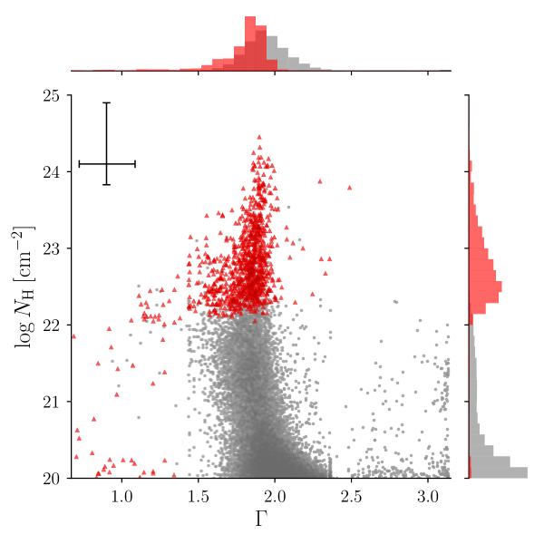
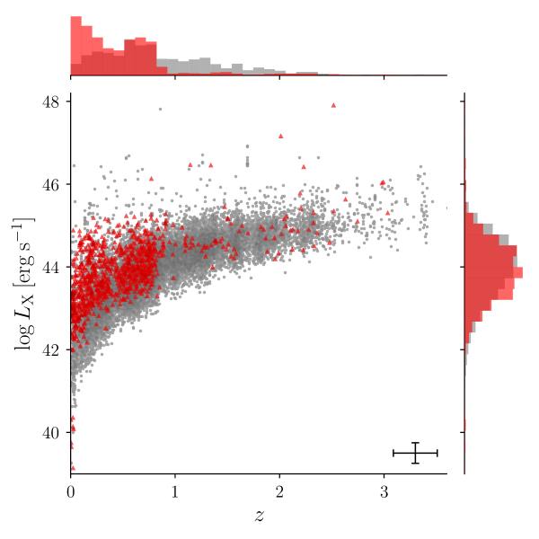
Figure 8: Photon index versus Hydrogen column density (left) and redshift versus 2–10 keV, absorption corrected luminosity (right) for detections classified as AGN with a reliable X-ray modelling (see Sect. 4). Red triangles are X-ray absorbed AGN; unabsorbed AGN are shown as grey circles. Errors are not included in the plots to improve visualization. Instead, we include error bars in the corners showing the median error of the corresponding parameters. The histograms in the upper and right side of the plots show the normalize distribution of the parameters for X-ray absorbed (red) and unabsorbed (grey).

It appears that there is an excess of absorbed sources at low redshift (see also Fig. 8). This is easily explained as the absorbed sources have a lower flux and thus they are detected at closer distances. The fraction of absorbed AGN remains roughly constant with luminosity, except for the highest luminosity bin, where the number of absorbed sources increases significantly. Although we emphasize that our sample is not statistically complete, but in contrast biased towards the brightest sources, regarding both the X-ray and the optical selection, we should not expect a strong correlation for the fraction of absorbed AGN with X-ray luminosity (see e.g. Sazonov et al., 2015).

The blue solid line in Fig. 7 shows the 2–10 keV luminosity distribution for all XMMFITCAT-Z sources classified as AGN, again based solely in their X-ray properties. There is a non-negligible high luminosity long tail for these sources, reaching X-ray luminosities above $10^{47}\leavevmode\nobreak\ \mathrm{erg\,s^{-1}}$. Such high luminosities are clearly nonphysical.

These results strongly suggest that our X-ray spectral modelling is overestimating the intrinsic 2–10 keV luminosity for some objects. We therefore tried to identify those sources with unreliable modelling.

There are two main effects that can overestimate the X-ray luminosity: On one hand, the photometric redshifts calculated for some sources could be wrong. For building XMMFITCAT-Z we did not apply any filtering regarding the quality of the photometric redshifts. In Ruiz et al. (2018) we presented several quality diagnostics for photo-z based on the shape of their probability density function. For example, by using the Peak Strength (PS) parameter included in XMMPZCAT we can select sources which photo-z probability distribution is narrowly concentrated around a single redshift, avoiding highly multimodal distributions. We considered objects with PS ¡ 0.7 as having an unreliable X-ray spectral modelling.

On the other hand, the complex models we used for sources with high counts (the absorbed double power-law model, “wapopo”, or the absorbed thermal plus power-law model, “wamekalpo”, see Sect. 2.3) can introduce artifacts in the X-ray modelling leading to nonphysical parameters: some of this sources are not well fitted by a single power low or thermal emission because they have a small but significant excess emission at the high energy end of the spectrum. This excess, that is associated with the AGN Compton reflection hump (Magdziarz & Zdziarski, 1995; Reynolds, 1999), can be easily modelled by introducing a highly absorbed power-law, with $N_{\mathrm{H}}\gtrsim 10^{23}\mathrm{cm^{-2}}$. When such artifact appears in the selected best-fit model, it can clearly overestimate the intrinsic 2–10 keV luminosity. Our selection criteria for X-ray absorbed sources will identify this kind of sources as highly absorbed, misinterpreting it as a heavily buried AGN component, but in fact they do not show any real spectral feature for X-ray absorption.

Hence, we classified as unreliable those X-ray sources well modelled using any of our complex models and classified as absorbed, but showing a 2–10 keV luminosity above $10^{45.3}\leavevmode\nobreak\ \mathrm{erg\,s^{-1}}$. This luminosity limit corresponds to the last luminosity bin in Fig. 6.

Finally, we also excluded sources with a loosely constrained $N_{\mathrm{H}}$ (i.e. the 90% credible interval for $\log N_{\mathrm{H}}$ is greater than 2 dex). Once we applied these quality criteria for selecting sources with a reliable X-ray modelling, we rejected 8871 detections: 444 absorbed AGN and 8427 unabsorbed AGN. Orange stars in Fig. 6 and the orange solid histogram in Fig. 7 include only AGN with reliable X-ray modelling. The figures clearly show that the effects due to overestimated luminosities disappear after applying this filtering.

In Fig. 8 we plot the Hydrogen column density against the Photon Index (left) and redshift against 2–10 keV luminosity (right) for detections classified as AGN in XMMFITCAT-Z (objects with unreliable X-ray modelling are not included), and the corresponding normalized distribution for each parameter. Grey circles correspond to unabsorbed objects (17 158 detections); X-ray absorbed objects are plotted as red triangles (977 detections).

The use of MIR colours is a common tool for AGN identification (Stern et al., 2005; Donley et al., 2007, 2012; Mateos et al., 2012; Assef et al., 2013), in particular by using data in the W1 ($3.4\>\mu m$) and W2 ($4.6\>\mu m$) bands from the WISE all-sky surveys (Wright et al., 2010; Mainzer et al., 2011; Cutri et al., 2013), since galaxies are expected to display bluer colors than AGN in the MIR. In Fig. 9 we present the W1–W2 distribution (lower panel) for XMMFITCAT-Z AGN with counterparts in the All-WISE catalogue (Cutri et al., 2013).

The W1–W2 colour has been proposed by Stern et al. (2005) as an efficient diagnostic for the selection of AGN. The idea is that the heated torus dust results in increased emission in the W2 band. MIR colors show no difference between absorbed and unabsorbed objects, as expected if the MIR emission is from the torus and hence inclination independent. We see that a considerable fraction of our sources is classified as AGN following the W1–W2 criterion. However, an almost equally large number of X-ray sources would not be classified as AGN following the W1–W2 criterion.

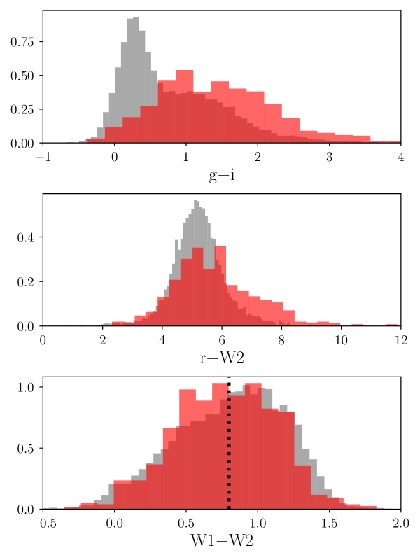
Figure 9: g–i (top), r–W2 (middle) and W1–W2 (bottom) normalized colour distributions. Solid, red histograms: unique sources classified as X-ray absorbed AGN in XMMFITCAT-Z; solid, grey histogram: X-ray unabsorbed AGN. Only AGN with reliable modelling are included (see discussion in Sect. 4). The vertical dotted line in the bottom panel shows the Stern et al. (2012) MIR criterion for AGN selection ($\mathrm{W1-W2}>0.8$).

These objects are associated with AGN where the galaxy starts to dominate over the AGN colours (see also Barmby et al., 2006). Assef et al. (2013) propose a more elaborate criterion where the W1–W2 cutoff is a function of the W2 magnitude. This selection curve (90% completeness) is shown in Fig. 10. It is evident that a significant number of X-ray selected AGN would evade identification if we used mid-IR colour criteria alone. In the same figure we plot the sources which were not classified as AGN in our spectral fits (i.e. objects having a good X-ray spectral fit with at least one of our models, but with 2–10 keV luminosity below $10^{42}\leavevmode\nobreak\ \mathrm{erg\,s^{-1}}$). The vast majority of these lie outside the AGN locus. This suggests that the X-ray spectral criteria alone are quite efficient in selecting AGN. As stated above, AGN selections based on WISE colours are efficient for identifying sources where the mid-IR torus emission dominates over the host galaxy contribution, that is, for luminous, unobscured AGN (see e.g. Eckart et al., 2010; Hickox et al., 2017; Pouliasis et al., 2020). Our results show how X-ray spectral criteria can select AGN with lower luminosities. Figure 10 also shows some contamination of sources within the AGN wedge but with no evidence in X-rays of hosting an AGN (light green crosses). Georgakakis et al. (2020) suggested that these sources can be star forming galaxies at redshift $\lesssim 0.5$ that scatter into the AGN MIR wedge due to the photometric uncertainties of the WISE magnitudes.

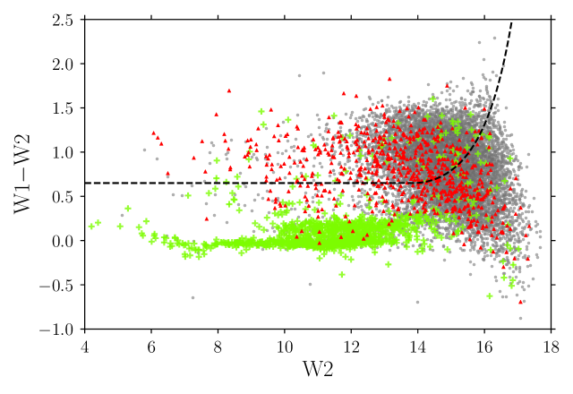
Figure 10: W2 versus W1–W2 for XMMFITCAT-Z unique sources with WISE counterparts. Red triangles show X-ray absorbed AGN; Grey circles show X-ray unabsorbed AGN. Light green crosses are objects not classified as AGN, but with an acceptable fit in XMMFITCAT-Z. Only sources with reliable modelling are included (see discussion in Sect. 4). The black, dashed line show the Assef et al. (2013) criterion for AGN selection.

Next, we discuss the obscuration properties of our sample. In the top panel of Fig. 9 we present the g–i colours of the absorbed vs. the unabsorbed sources. X-ray absorbed sources are optically redder compared to unabsorbed sources, as expected. However, there is a non-negligible number of X-ray unabsorbed sources with very red colours. Part of them could be missed absorbed objects, but they could be also truly peculiar sources. The catalogue is then quite useful to identify this kind of objects for further studies.

In the middle panel of Fig. 9 we present the r–W2 colour distribution. Yan et al. (2013) suggested that this colour (r–W2 ¿ 6) offers a powerful diagnostic for the selection of obscured AGN, in combination with pure MIR diagnostics to identify AGN (W1–W2 ¿ 0.8 and W2 ¡ 15.8) This is because in the presence of reddening, the r band is easily diminished while the W2 emission remains relatively unscathed. As expected the X-ray obscured sources have a redder tail compared to the unobscured sources. It is worth noting however, that a considerable fraction of X-ray unabsorbed sources have r–W2 ¿ 6. Hickox et al. (2017) show that the r–W2 criterion is only really effective above $z>1$. The fact that the bulk of our absorbed AGN is below redshift one (see Fig. 8, right panel) can explain our result.

Our analysis of XMMFITCAT-Z sources is consistent with many previous studies (Eckart et al., 2010; Stern et al., 2012; Assef et al., 2013; Yan et al., 2013; Mateos et al., 2012, 2013; Mountrichas et al., 2017b, 2020; Pouliasis et al., 2020) showing that MIR diagnostics are powerful for the identification of luminous AGN, but they fail for AGN with lower luminosity and/or mild absorption, where the stellar contribution to the optical/MIR emission is non-negligible. By focusing on the X-ray properties, we can identify these objects.

5 Summary

We present a catalogue of automated X-ray spectral fits, using the 3XMM-DR6 spectral products. Photometric redshifts have been previously estimated (Ruiz et al., 2018) using machine learning techniques (TPZ; Carrasco Kind & Brunner, 2013). 22677 X-ray sources are presented with a reasonable quality X-ray spectrum, meaning that each XMM-Newton detector have over 50 counts, and with available photometric or spectroscopic redshift. The X-ray spectral fits have been performed using Bayesian X-ray analysis (Buchner et al., 2014), including the PDF of photometric redshift as priors.

As a brief demonstration of the potential of this X-ray spectral catalogue, we present the properties of the 765 sources showing strong evidence of being X-ray absorbed AGN. We show that a considerable fraction of our sample would not be classified as AGN based on their mid-IR colours, W1–W2 vs. W2. About one third of the X-ray absorbed AGN presents red $\rm r-W2>6$ colours. It appears then that the r–W2 criterion, often used in the literature for the selection of obscured AGN, produces very different samples compared to the X-ray criteria based on the hydrogen column density.

Appendix A Description of the XMMFITCAT-Z

The XMMFITCAT-Z table contains one row for each detection, and 157 columns containing information about the source detection and the spectral-fitting results. Not available values are represented by an empty ”NULL” value. The first 14 columns contain information about the source and observation, including redshift information, whereas the remaining 143 columns contain, for each model applied, spectral-fit flags, parameter values and errors, fluxes, luminosities, and five columns to describe the goodness of the fit.

1. Source and observation

   • IAUNAME: The IAU name assigned to an unique source in the 3XMM-DR6 catalogue.

   • SC_RA, SC_DEC: Right ascension and declination in degrees (J2000) of the unique source, as in the 3XMM-DR6 catalogue. RA and DEC correspond to the SC_RA and SC_DEC columns in the 3XMM-DR6 catalogue. These are corrected source coordinates and, in the case of multiple detections of the same source, they correspond to the weighted mean of the coordinates for the individual detections.

   • SRCID: A unique number assigned to a group of catalogue entries which are assumed to be the same source in 3XMM-DR6.

   • DETID: A consecutive number which identifies each entry (detection) in the 3XMM-DR6 catalogue.

   • OBS_ID: The XMM-Newton observation identification, as in 3XMM-DR6.

   • SRC_NUM: The (decimal) source number in the individual source list for this observation (OBS_ID), as in 3XMM-DR6. In the pipeline products this number is used in hexadecimal form.

   • PHOT_Z, PHOT_ZERR: Photometric redshift of the source (from XMMPZCAT) and the corresponding $1\sigma$ error.

   • SPEC_Z: Spectroscopic redshift of the source, if available.

   • T_COUNTS/H_COUNTS/S_COUNTS: spectral background subtracted counts in the full/hard/soft bands computed by adding all available instruments and exposures for the corresponding observation.

   • NHGAL: Galactic column density in the direction of the source from the Leiden/Argentine/Bonn (LAB) Survey of Galactic HI.

2. Model related columns
   Columns referring to any particular model start with the model’s name (wapo, wamekal, wamekalpo, wapopo).

   1. Spectral-fit summary columns

      • A_FIT: The value is set to True, if an acceptable fit, i.e. KS p-value $>0.01$, has been found for at least one of the models applied, and to False otherwise.

      • P_MODEL: The data preferred model, that is the model with the highest evidence (lowest logZ). A spectral model is always listed regardless of the fit being an acceptable or an unacceptable fit.

      • A_MODELS: List of acceptable models. This column contains the remaining models with relative evidence (with respect to P_MODEL) lower than 30 (’very strong evidence’ accordingly to the scale of Jeffreys 1961). Assuming all models a priori equally probable, there is no statistical reason to rule out any of the models in the set formed by P_MODEL and A_MODELS. Hence, if the fit is acceptable, the simplest model should be selected as the best-fit model.

   2. Parameters and errors.
      Columns referring to parameters and errors start with the model name and the parameter name (logNH[1,2], PhoIndex[1,2], kT, and z). Values for the normalizations of the models and the relative normalization factors between instruments are not included in the table (but they are available in the SQL database).

      • ¡MODEL¿_¡PARAMETER¿: parameter value.

      • ¡MODEL¿_¡PARAMETER¿_min, ¡MODEL¿_¡PARAMETER¿_max: upper and lower limits of the 90% credible interval for the parameter.

   3. Fluxes and luminosities.

      • ¡MODEL¿_flux_¡BAND¿: the mean observed flux (in erg cm^-2 s^-1) of all instruments and exposures for the corresponding observation, in ¡BAND¿ (soft/hard). Observed fluxes were corrected of Galactic absorption.

      • ¡MODEL¿_fluxmin_¡BAND¿, ¡MODEL¿_fluxmax_¡BAND¿: lower and upper limits of the 90% credible interval.

      • ¡MODEL¿_intflux_¡BAND¿: the mean intrinsic flux (rest-frame, corrected of intrinsic absorption, in erg cm^-2 s^-1) of all instruments and exposures for the corresponding observation, in ¡BAND¿ (soft/hard).

      • ¡MODEL¿_intfluxmin_¡BAND¿, ¡MODEL¿_intfluxmax_¡BAND¿: lower and upper limits of the 90% credible interval.

      • ¡MODEL¿_lumin_¡BAND¿: the mean luminosity (rest-frame, corrected of intrinsic absorption, in erg s^-1) of all instruments and exposures for the corresponding observation, in ¡BAND¿ (soft/hard).

      • ¡MODEL¿_luminmin_¡BAND¿, ¡MODEL¿_luminmax_¡BAND¿: lower and upper limits of the 90% credible interval.

   4. Fitting statistics.

      • ¡MODEL¿_wstat: W-stat (Cash statistics) value.

      • ¡MODEL¿_dof: Degrees of freedom.

      • ¡MODEL¿_ks: Kolmogorov-Smirnov (KS) statistic.

      • ¡MODEL¿_ks_pvalue: KS p-value.

      • ¡MODEL¿_logZ: Natural logarithm of the evidence, estimated by the MultiNest algorithm.

References

- Assef et al. (2013) Assef, R. J., Stern, D., Kochanek, C. S., et al. 2013, ApJ, 772, 26
- Astropy Collaboration et al. (2018) Astropy Collaboration, Price-Whelan, A. M., Sipőcz, B. M., et al. 2018, AJ, 156, 123
- Barcons et al. (2007) Barcons, X., Carrera, F. J., Ceballos, M. T., et al. 2007, A&A, 476, 1191
- Barmby et al. (2006) Barmby, P., Alonso-Herrero, A., Donley, J. L., et al. 2006, ApJ, 642, 126
- Buchner et al. (2014) Buchner, J., Georgakakis, A., Nandra, K., et al. 2014, A&A, 564, A125
- Carrasco Kind & Brunner (2013) Carrasco Kind, M. & Brunner, R. J. 2013, MNRAS, 432, 1483
- Cash (1979) Cash, W. 1979, ApJ, 228, 939
- Corral et al. (2014) Corral, A., Georgantopoulos, I., Watson, M. G., et al. 2014, A&A, 569, A71
- Corral et al. (2015) Corral, A., Georgantopoulos, I., Watson, M. G., et al. 2015, A&A, 576, A61
- Cutri et al. (2013) Cutri, R. M., Wright, E. L., Conrow, T., et al. 2013, VizieR Online Data Catalog, 2328
- Della Ceca et al. (2004) Della Ceca, R., Maccacaro, T., Caccianiga, A., et al. 2004, A&A, 428, 383
- Donley et al. (2012) Donley, J. L., Koekemoer, A. M., Brusa, M., et al. 2012, ApJ, 748, 142
- Donley et al. (2007) Donley, J. L., Rieke, G. H., Pérez-González, P. G., Rigby, J. R., & Alonso-Herrero, A. 2007, ApJ, 660, 167
- Eckart et al. (2010) Eckart, M. E., McGreer, I. D., Stern, D., Harrison, F. A., & Helfand, D. J. 2010, ApJ, 708, 584
- Fabian (2006) Fabian, A. C. 2006, in ESA SP-604: The X-ray Universe 2005, ed. A. Wilson, 463
- Fabian et al. (2000) Fabian, A. C., Iwasawa, K., Reynolds, C. S., & Young, A. J. 2000, PASP, 112, 1145
- Feroz et al. (2009) Feroz, F., Hobson, M. P., & Bridges, M. 2009, MNRAS, 398, 1601
- Freeman et al. (2001) Freeman, P., Doe, S., & Siemiginowska, A. 2001, in Proc. SPIE, ed. J. L. Starck & F. D. Murtagh, Vol. 4477, 76–87
- Georgakakis et al. (2020) Georgakakis, A., Ruiz, A., & LaMassa, S. M. 2020, MNRAS, 499, 710
- Haardt & Maraschi (1991) Haardt, F. & Maraschi, L. 1991, ApJ, 380, L51
- Haardt et al. (1994) Haardt, F., Maraschi, L., & Ghisellini, G. 1994, ApJ, 432, L95
- Hickox et al. (2017) Hickox, R. C., Myers, A. D., Greene, J. E., et al. 2017, ApJ, 849, 53
- Ho (1999) Ho, L. C. 1999, ApJ, 516, 672
- Jansen et al. (2001) Jansen, F., Lumb, D., Altieri, B., et al. 2001, A&A, 365, L1
- Jeffreys (1961) Jeffreys, H. 1961, The Theory of Probability, Texts in the Physical Sciences (Oxford Univ. Press)
- Kalberla et al. (2005) Kalberla, P. M. W., Burton, W. B., Hartmann, D., et al. 2005, A&A, 440, 775
- Magdziarz & Zdziarski (1995) Magdziarz, P. & Zdziarski, A. A. 1995, MNRAS, 273, 837
- Mainzer et al. (2011) Mainzer, A., Bauer, J., Grav, T., et al. 2011, ApJ, 731, 53
- Mateos et al. (2013) Mateos, S., Alonso-Herrero, A., Carrera, F. J., et al. 2013, MNRAS, 434, 941
- Mateos et al. (2012) Mateos, S., Alonso-Herrero, A., Carrera, F. J., et al. 2012, MNRAS, 426, 3271
- Menzel et al. (2016) Menzel, M.-L., Merloni, A., Georgakakis, A., et al. 2016, MNRAS, 457, 110
- Motch et al. (2017) Motch, C., Carrera, F., Genova, F., et al. 2017, in Astronomical Society of the Pacific Conference Series, Vol. 512, Astronomical Data Analysis Software and Systems XXV, ed. N. P. F. Lorente, K. Shortridge, & R. Wayth, 165
- Mountrichas et al. (2017a) Mountrichas, G., Corral, A., Masoura, V. A., et al. 2017a, A&A, 608, A39
- Mountrichas et al. (2020) Mountrichas, G., Georgantopoulos, I., Ruiz, A., & Kampylis, G. 2020, MNRAS, 491, 1727
- Mountrichas et al. (2017b) Mountrichas, G., Georgantopoulos, I., Secrest, N. J., et al. 2017b, MNRAS, 468, 3042
- Mushotzky et al. (1995) Mushotzky, R. F., Fabian, A. C., Iwasawa, K., et al. 1995, MNRAS, 272, L9
- Nandra & Pounds (1994) Nandra, K. & Pounds, K. A. 1994, MNRAS, 268, 405
- Netzer et al. (1998) Netzer, H., Turner, T. J., & George, I. M. 1998, ApJ, 504, 680
- Panessa et al. (2007) Panessa, F., Barcons, X., Bassani, L., et al. 2007, in American Institute of Physics Conference Series, Vol. 924, The Multicolored Landscape of Compact Objects and Their Explosive Origins, ed. T. di Salvo, G. L. Israel, L. Piersant, L. Burderi, G. Matt, A. Tornambe, & M. T. Menna, 830–835
- Pineau et al. (2017) Pineau, F.-X., Derriere, S., Motch, C., et al. 2017, A&A, 597, A89
- Planck Collaboration et al. (2016) Planck Collaboration, Ade, P. A. R., Aghanim, N., et al. 2016, A&A, 594, A13
- Pouliasis et al. (2020) Pouliasis, E., Mountrichas, G., Georgantopoulos, I., et al. 2020, MNRAS, 495, 1853
- Reynolds (1999) Reynolds, C. S. 1999, in Astronomical Society of the Pacific Conference Series, Vol. 161, High Energy Processes in Accreting Black Holes, ed. J. Poutanen & R. Svensson, 178
- Robert et al. (2009) Robert, C. P., Chopin, N., & Rousseau, J. 2009, Statist. Sci., 24, 141
- Robertson & Cryer (1974) Robertson, T. & Cryer, J. 1974, Journal of the American Statistical Association, 69, 1012
- Rosen et al. (2016) Rosen, S. R., Webb, N. A., Watson, M. G., et al. 2016, A&A, 590, A1
- Ruiz et al. (2018) Ruiz, A., Corral, A., Mountrichas, G., & Georgantopoulos, I. 2018, A&A, 618, A52
- Sazonov et al. (2015) Sazonov, S., Churazov, E., & Krivonos, R. 2015, MNRAS, 454, 1202
- Scargle et al. (2013) Scargle, J. D., Norris, J. P., Jackson, B., & Chiang, J. 2013, ApJ, 764, 167
- Stern et al. (2012) Stern, D., Assef, R. J., Benford, D. J., et al. 2012, ApJ, 753, 30
- Stern et al. (2005) Stern, D., Eisenhardt, P., Gorjian, V., et al. 2005, ApJ, 631, 163
- Turner & Miller (2009) Turner, T. J. & Miller, L. 2009, A&A Rev., 17, 47
- Wright et al. (2010) Wright, E. L., Eisenhardt, P. R. M., Mainzer, A. K., et al. 2010, AJ, 140, 1868
- Yan et al. (2013) Yan, L., Donoso, E., Tsai, C.-W., et al. 2013, AJ, 145, 55