Analysis of COVID-19 evolution in Senegal: impact of health care capacity
Abstract
We consider a compartmental model from which we incorporate a time-dependent health care capacity having a logistic growth. This allows us to take into account the Senegalese authorities response in anticipating the growing number of infected cases. We highlight the importance of anticipation and timing to avoid overwhelming that could impact considerably the treatment of patients and the well-being of health care workers. A condition, depending on the health care capacity and the flux of new hospitalized individuals, to avoid possible overwhelming is provided. We also use machine learning approach to project forward the cumulative number of cases from March 02, 2020, until 1st December, 2020.
keywords:
COVID-19, health care capacity, parameter estimates, logistic growth, forecasting, machine learning.1 Introduction
COVID-19, declared a pandemic by the World Health Organization (WHO) [25] on 11 March 2020, is still spreading around the world up to date 26 September 2020. The number of people infected is beyond 32 million on 26 September 2020 with 989,380 deaths [24]. In Senegal, the number of cumulative cases is currently 14839 with 2624 individuals undergoing treatment on 25 September 2020[13]. The first cases, from Wuhan, were notified to WHO on 31 December 2019 [25, 26] while, Senegal notified its first case on 02 March 2020 [13]. Because of its limited resources, as in many sub-Saharan African countries, it is therefore valuable to understand the growth and the timing in responding to the logistic needs of their health system. We note that several developed countries that nevertheless have high-capacity health structures have been overwhelmed and this considerably impacted negatively in the combat against the pandemic. In [14] it is discovered that the growing number of COVID-19 cases in the United States could gravely challenge the critical care capacity, thereby exacerbating case fatality rates. As pointed out in [23], under-resourced health systems may pose a threat to patient care as well as the safety and well-being of health care workers.
From the appearance of the first cases of COVID-19, the Senegalese authorities decided to anticipate by increasing gradually the capacity of its hospitals to take care of patients suffering from COVID-19. One of the aims of the present paper is to study different scenarios of involution of the number of virus patients by varying the growth rate and the number of, say, beds or rooms.
As an approach, we use a mathematical model that integrates the different stages of individuals (Susceptible, Exposed, Asymptomatic, Symptomatic, Removed) with the parameters depending on the health resources availability.
To this cope, we consider a modified SEWIR model [16] in which we include a time-dependent carrying capacity representing the evolution of the Senegalese hospitals’ capacity in response to the growing number of cases in Senegal.
Our analysis highlights the importance of anticipation and timing to avoid overwhelming in the health system. More precisely, our analysis shows, in particular, that, while the epidemic growths exponentially fast, by respecting a certain logistic growth (at which the number of beds is being added) in the health system, the epidemic might remain under control. As a consequence, a non-negligible number of expenses can be saved.
Finally, a machine learning approach to project forward the cumulative number of virus infected cases is provided. Let us mention that several studies have been conducted in different contexts to assess the impact of hospital saturation in COVID-19. We refer for examples to [5, 7, 8, 14, 21] and the references therein.
Our work complements several studies that have been carried out on the spread of Sars-CoV-2 in Senegal [2, 3, 4, 6, 15, 16, 17, 18]. It should be noted that the aforementioned studies did not address the impact of saturation on patients care in Senegal. However, some studies on the prediction of the number of new cases for Senegal have already been carried out using machine learning [2, 3, 15, 16] and on the impact of contaminated objects using compartmental models [6].
The paper is organized as follows. In section 2, we describe in detail our model as well as the parameters involved. It is followed by Section 3 concerning the estimation of the unknown parameters. In section 4 we derive the time-dependent effective reproduction number which is a key function that informs about the impact of the various decisions taken by the authorities during the epidemic. In Section 5, we first present the calibration of the model to the cumulative number of reported cases. We then present numerical simulations on the impact of the dynamics of health capacity on the patients care. Finally, in Section 6, we use machine learning to project forward the number of cumulative cases until 1st December 2020.
2 Model description
We consider compartmental epidemic model that incorporates a time-dependent carrying capacity of health structures for the treatment of COVID-19 patients at the hospitals. The model reads as follow
| (2.1) |
with initial conditions
| (2.2) |
and
| (2.3) |
The state variable is the number of susceptible individuals at time , the number of exposed individuals at time and the number of waiting cases for confirmation (with infectiousness) at time . The number of confirmed and monitored cases at time is denoted by . The variable describes the effective carrying capacity of the health structure, which is the maximum number of individuals that can be correctly monitored. Finally represents the removed individuals at time due to death or recovery. The figure below represents the diagram flux of the model.
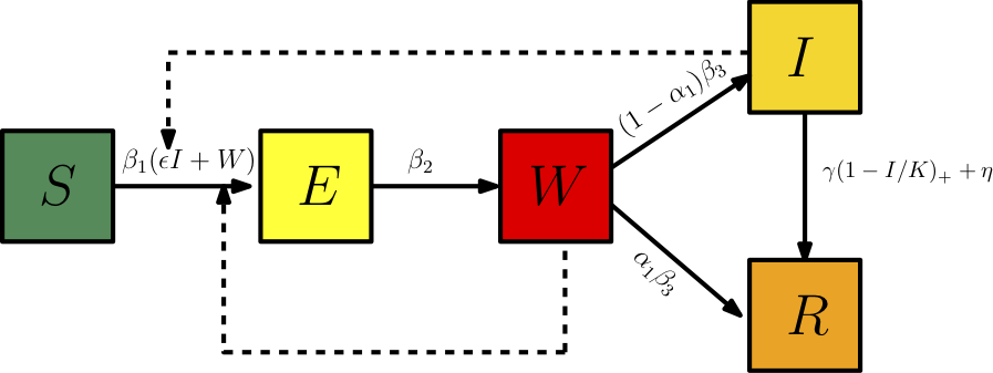
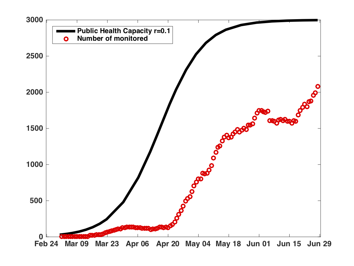
The term represents the transmission of the disease within the health structures where can be interpreted as the probability that a susceptible individual is working in the health system. More precisely we set with the number of health care workers and the initial number of susceptible individuals. The quantity of is the average incubation period. We assume that the average waiting time for confirmation is days. After the waiting time, a fraction is monitored while the remaining fraction is removed due to death or recovered. The removal rate of the confirmed cases is described by in order to take into account the saturation effect of the public health structures. The term which is a decreasing function of describes the efficiency of the health structures. The maximal efficiency is while the minimal efficiency is reached when the number of confirmed cases becomes greater than the carrying capacity . In our modeling procedure, we have introduced a time-dependent carrying capacity which is motivated by the fact that in Senegal, the carrying capacity of the health structures was gradually increased in response to the increase in the number of infected individuals. The dynamics of the increase in the number of beds remains unknown because only announcements have been made. We chose a logistic equation to mimic the growth of the public health capacity to its saturation. Indeed, from the onset of the epidemic, the authorities announced a carrying capacity of 30 which gradually increased according to the number of cases. The maximum capacity of the structures remains unknown but in view of the announcements made, we assume that it is approximately 3000. The growth rate of is chosen such that it increases from on 02 March to approximately on 10 June and that the number of hospitalized individuals is below the effective carrying capacity. There are other possibilities of choosing the growth rate but the value appears to give the best fit to the data. The figure below describes the evolution of with respect to time and the evolution of the number of hospitalized individuals.
The evolution of the public health capacity and number of monitored are illustrated in Figure 2.
More precisely the dynamic of the carrying capacity is given by:
| (2.4) |
with
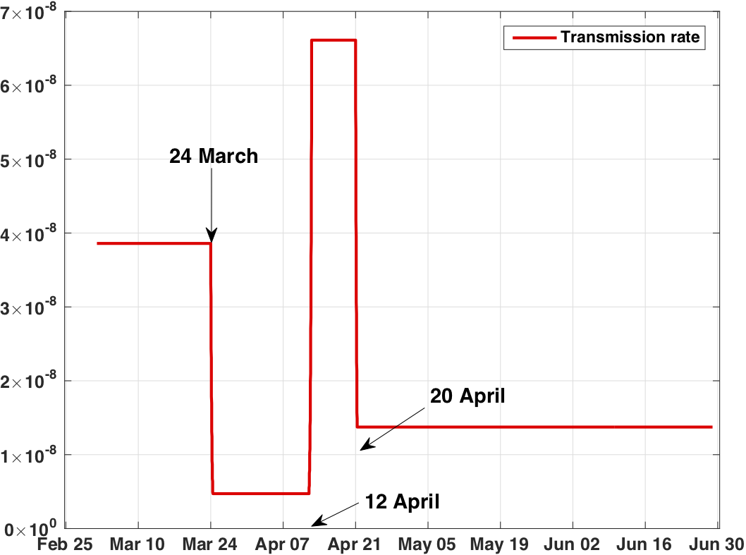
The parameter will serve to explore different scenarios in which the efforts of increasing health capacities are aborted. In model (2.1)-(2.4), we use a time-dependent transmission rate to take into account the various events that have impacted the spread of disease. Indeed several government actions such as partial lockdown, social distancing, interurban traffic ban, border closure have impacted the progression of the disease. The time-dependent transmission rate has the following form
| (2.5) |
where the parameters are estimated by using the data on reported cases. More precisely we have
with March the date at which the first case was reported [13], March, April and April. We distinguish three phases. Phase takes place between the dates 02 March, the beginning of the epidemic, until the first government actions at date March. Phase 2 which begins at , the date on which decisions such as public closing, interurban traffic ban, border closure were taken, is ended at date April. The date corresponds to a sudden increase in the number of cases with a decline on approximately date April where Phase 3 began and cover the period of April to June the date at which we stop our study. The cause of the sudden increase in April remains unknown to us at this time. More accurate data would be needed in order to understand the advent of this phenomenon. However, we can follow the evolution of the dynamics of the epidemic using the time-dependent transmission rate. The parameter describes the intensity of the government actions or sudden events that impacted the transmission rate. We refer to [10] where such interpretation has been used to describes the government actions. The parameters , and allow us to measure the impact of each phase on the transmission rate . The values of the parameters , estimated in Section 3 are
| (2.6) |
and the estimated value of in Section 3 is
| (2.7) |
The figure below describes the transmission rate .
Next we summarize the descriptions of the remaining symbols in the table below.
| Symbol | Description | Method | |
|---|---|---|---|
| Onset of the epidemic | fixed | ||
| Number of susceptible at time | fixed | ||
| Number of exposed individuals at time | fitted | ||
| Number of wating individuals at time | fitted | ||
| Number of monitored infectious at time | fitted | ||
| Transmission rate | fitted | ||
| average latent period | fixed | ||
| Removal rate of the wating individuals | fixed | ||
| Fraction of wating individuals that become monitored | fitted | ||
| Rate at which monitored individuals are removed at hospital saturation | fixed | ||
| Maximal removal rate of the monitored individuals | fixed | ||
| Maximal hospital carrying capacity | fixed | ||
| Intrinsic growth rate of the hospital carrying capacity | fixed | ||
| Number of healthcare worker per susceptible individual | fixed |
The values of fixed parameters in Table 1 are given in the next table
3 Parameter estimates using the early phase
In this section, will use the approach developed in [9, 10, 11, 12] in order to estimate the parameters from the early phase of the epidemic. Let be the cumulative number of reported cases at time be defined by
| (3.1) |
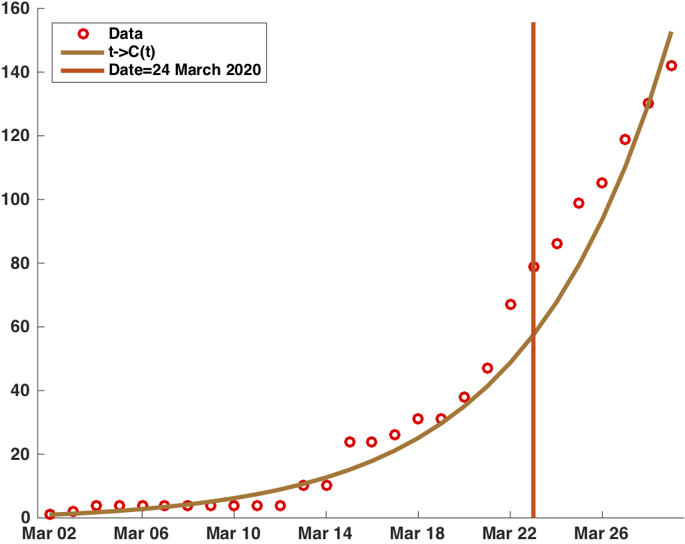
with Mars the date of the first reported cases in Senegal so that . The early phase of the epidemic corresponds to the period from the announcement of the first case on Mars to the first government actions at March . In this phase we assume that the number of infected individuals growth exponentially. Hence with such assumption, the cumulative number of cases has the following form
| (3.2) |
The Figure 4 below shows the comparison between the and the data from March until March that allows us to estimate the parameters and to
| (3.3) |
Assuming that is approximately equal to in the short time interval and that for each
and
it follows that we have the following approximation for a short time period
| (3.4) |
Furthermore differentiating (3.1) and (3.2) with respect to we obtain
that is
| (3.5) |
Solving the second and the third equation of (3.4) we get:
| (3.6) |
Plugging (3.5) and (3.6) into the first equation of (3.4), it follows that
| (3.7) |
Therefore using (3.3) together with (3.5)-(3.7) and the values of the parameters of Table 1 we obtain
| (3.8) |
and
| (3.9) |
In order to obtain the values of the parameters , that appear in the transmission rate we perform a curve fitting by using the data from March until June . The estimated values are listed below
4 The effective reproduction number
The effective reproduction number, , is the expected number of secondary cases produced by one typical infection joining a healthy population during its infectious period while the time-dependent effective reproduction number is the instantaneous transmissibility of the disease at time . The time-dependent effective reproduction number allows to follow the evolution of the epidemic as the time evolves in particular how is far above or far below .
In order to obtain we note that is the number of new infections per unit of time generated by one infectious individual. Thus assuming approximately constant during , it follows that the term
is the average number of new infections generated by one infectious individual (W) during its period of infectiousness . Moreover one infectious individual (W) generates on average
infectious individual(s) (I). Those infectious (I) has a maximum mean infectiousness period so that they generate
new infections after times.
We finally define the time-dependent effective reproduction number as
| (4.1) |
The figure below gives the evolution of the effective reproduction number.
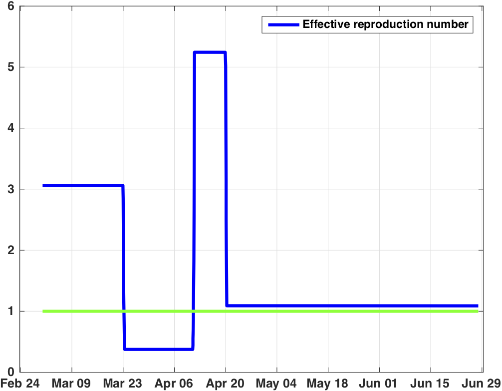
We observe that the effective reproduction number is larger than (approximately ) during the early phase of the epidemic that is from 02 March to 24 March and is smaller than during the second Phase. We can therefore observe that the first actions of the government had a positive effect on the spread of the epidemic because it tended to disappear if the effective measures would have been kept in the same trend. However, the sudden increase in cases on April 12th impacted the effective reproduction number to bring it to around 5. It goes down until it is close to but greater than 1 from April 20th. The cause of this increase is unknown to us but a better knowledge of the data may allow us to find an explanation.
5 Numerical simulations
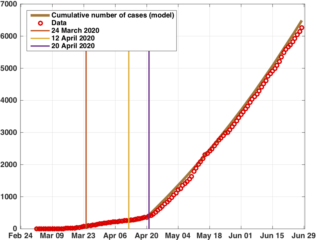
In this section we perform numerical simulations of the dynamics of the spread of the COVID-19 epidemic based on our proposed model (2.1)-(2.4). We consider the regions of Dakar, Thies and Diourbel which concentrate around 95% of the reported cases. To do so we assume that the initial number of susceptibles is the population of Dakar, Thies and Diourbel, that is to say [1]. The values of the parameters of the model are listed in Table 2. The time-dependent transmission rate is given in (2.5)-(2.7) while the estimated initial conditions in Section 3 are . In Figure 6 below we compare the cumulative number of cases defined in (3.1) with of the cumulative number of reported cases showing that our model agrees with the data.
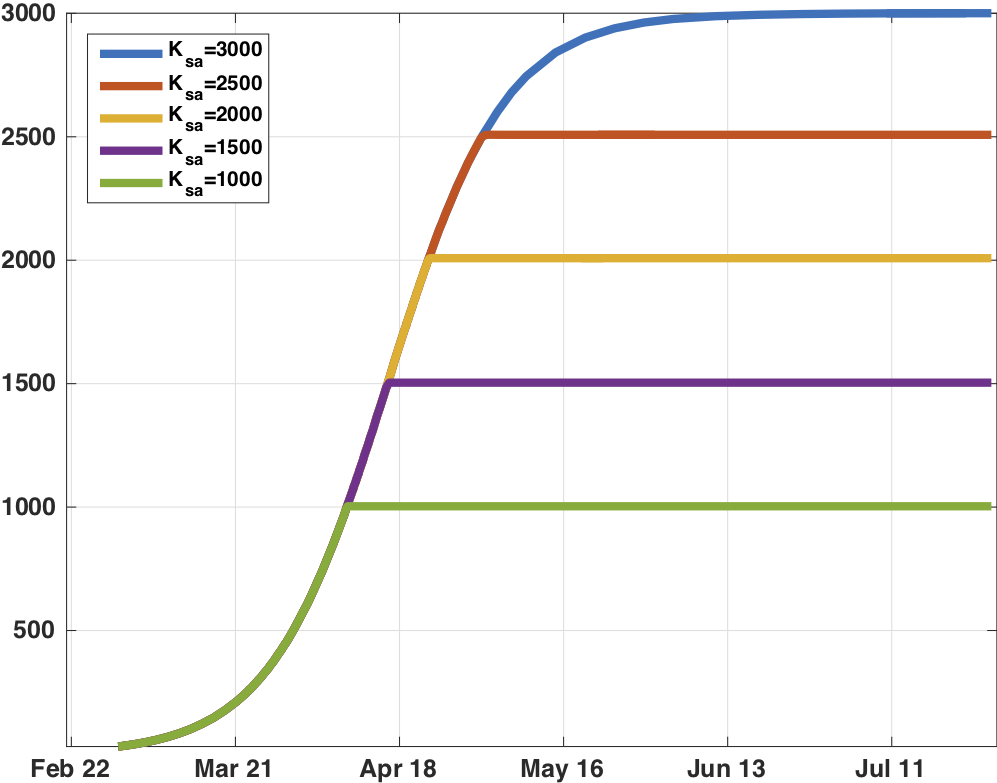
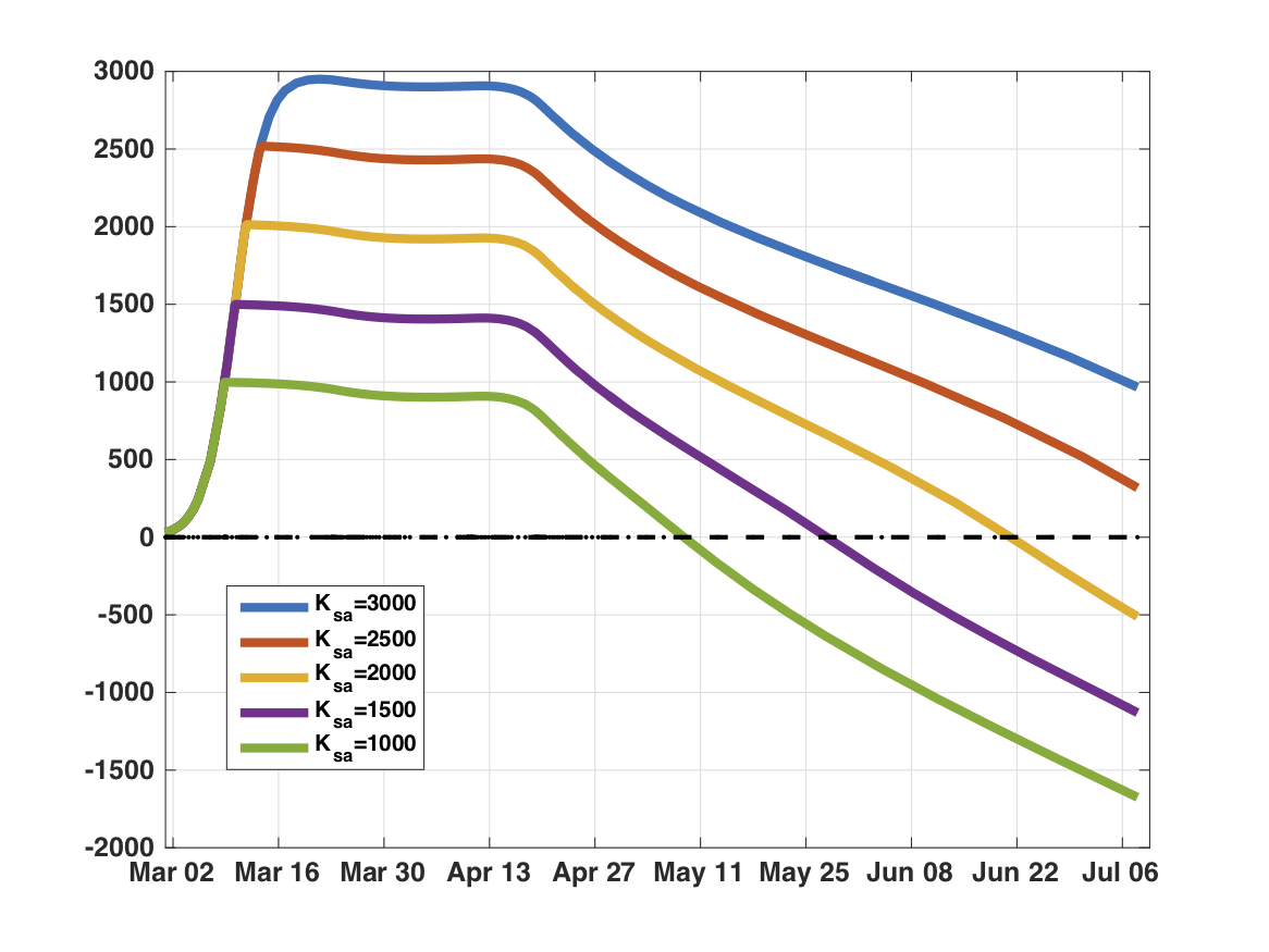
In order to illustrate the impact of the saturation of health structures on the number of monitored individuals, we consider several scenarios. Indeed, we consider the same evolution of the reception capacity with interruptions in growth at predefined values. More precisely we consider the following dynamic
| (5.1) |
where , the saturation level, is respectively , , , and and is illustrated by the following figure.
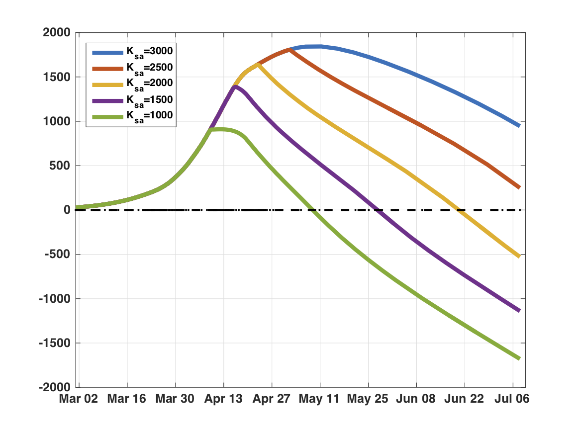
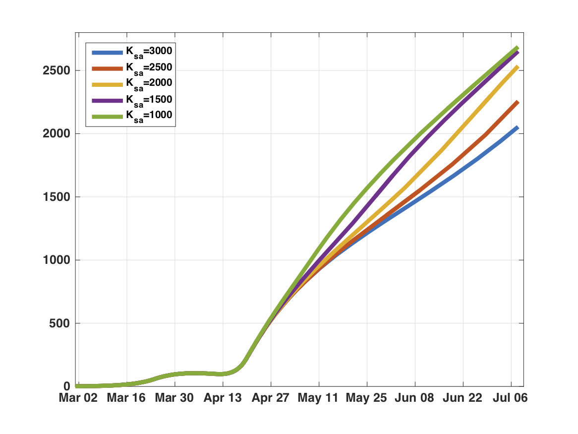
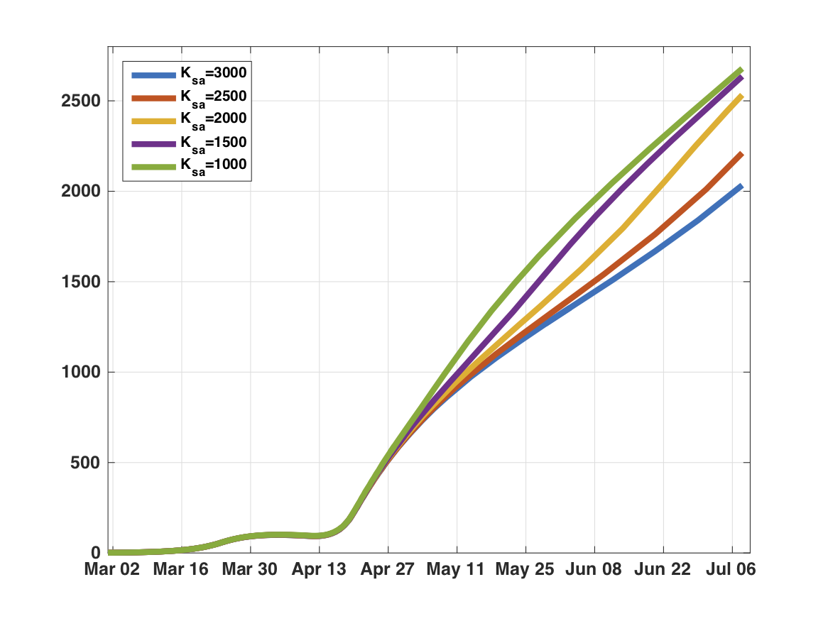
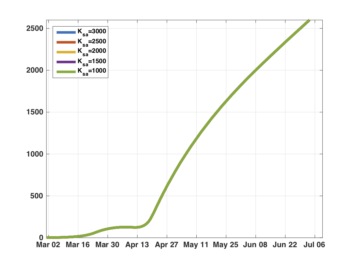
In Figure 8 we plot the corresponding number of monitored individuals that is when the dynamics of the carrying capacity is given by (5.1) with , , , and while the growth rate is fixed at . We see that the epidemic is under control, until 28 June only when and . This shows that the maximum value of the carrying capacity, , may impact significantly the efficiency of public health structures by slowing down the rate at which individuals are removed from the hospital. In Figure 9 we look at the influence of the growth rate on the number of monitored individuals. We see that increasing from to , does not impact significantly the number of monitored individuals and the dates at which overwhelming occurs. This is the case for all values of .
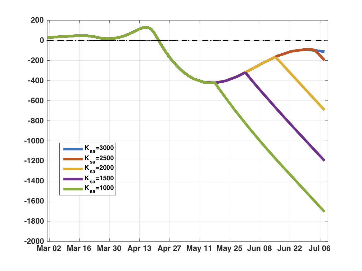
For , Figure 10, we see that the number of monitored individuals becomes larger than the maximum number of available resources at the early stage of the epidemic, around 20 April. We also observe that remains unchanged for different values of . Thus our model captures and validates the obvious fact that the faster you increase the number of beds, the better you can handle the hospitalized people. Figure 10 emphasizes more the sensibility of the growth rate which can also be seen/interpreted as the timing in anticipating overwhelming. Indeed we observe that for the maximal value of resources , stay larger than until 28 June for while for we see that the number monitored becomes larger than available resources from mid-April to the end of June.
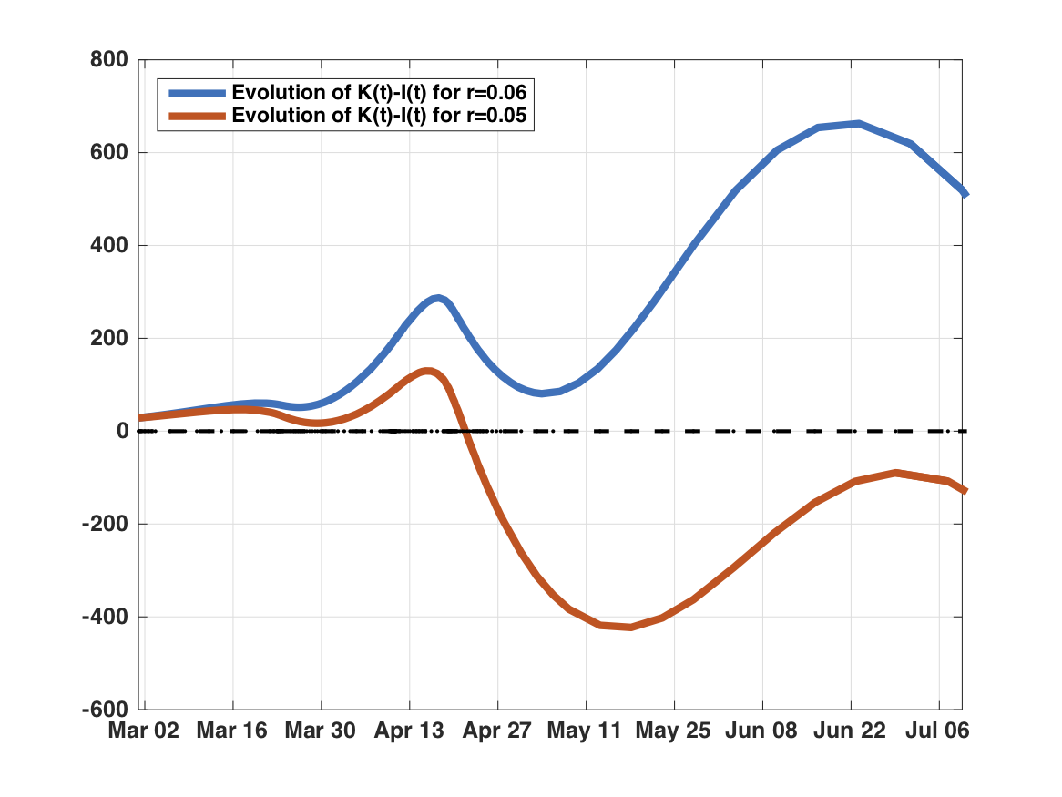
In view of our discussion, it would be important to have a condition that guarantees the unsaturation of health structures. It is contained in the following
Lemma 5.1.
Assume that . Assume in addition that is increasing and differentiable with respect to . If
| (5.2) |
for some then we have
Proof.
Define
Then, by assumption and by continuity there is such that for each . Define
Next, we show that . Assume by contradiction that . Then we have that is so that by (5.2)
This means that is locally strictly increasing from which contradict the definition of . ∎
Remark 5.2.
Let us note that condition (5.2) can be used in practice. Indeed is known and is the flux of new monitored individuals which is bounded above by the daily number of COVID-19 positive tests. Since is a controllable quantity, the condition (5.2) may serve to anticipate an overwhelming over time.
It is important to note that in the above Lemma, we do not require to have logistic growth. We only require to be an increasing function.
6 Machine learning for forecasting
In this section, we present a machine learning approach for the forecasting of the cumulative number of confirmed cases .
First, we collect the pandemic data from [13], from March 02, 2020, to October 22, 2020. Then, we perform a forecast with Prophet to predict the final size of coronavirus epidemy
The numerical tests are performed by using Python with the Panda library
[20], and were executed on a computer with the following characteristics: intel(R) Core-i7 CPU 2.60GHz, 24.0Gb of RAM, under the UNIX system.
6.1 Prophet model
Prophet [19, 22], is a procedure for forecasting time series data based on an additive model where non-linear trends are fit with yearly, weekly, and daily seasonality, plus holiday effects. It works best with time series that have strong seasonal effects and several seasons of historical data. Prophet is robust in dealing with missing data and shifts in the trend and typically handles well outliers. For the averaging method, the forecasts of all future values are equal to the average (or “mean”) of the historical data. If we let the historical data be denoted by , then we can write the forecasts as
The notation is a short-hand for the estimate of based on the data .
A forecasting interval gives an interval within which we expect to lie on, with a specified probability. For example, assuming that the forecast errors are normally distributed, a 95% forecasting interval for the -step forecast is
where is an estimate of the standard deviation of the -step forecast distribution.
6.1.1 Diagnostics
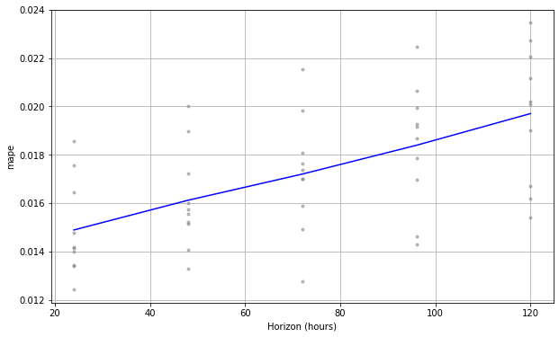
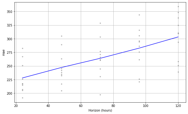
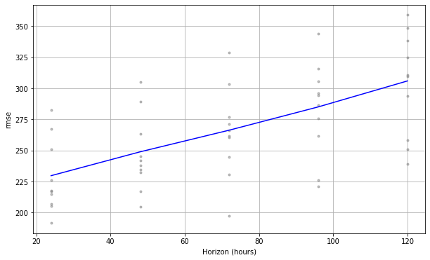
Here, we make some diagnostics by using the cross validation (see Table 3) and the performance metrics (see Table 4) using mse, rmse, mae and mape. The Figure 15 illustrate these cross validation metrics, making 10 forecasts with cutoffs between 2020-10-08, 00:00:00 and 2020-10-17, 00:00:00 (initial=’220 days’, period=’1 days’, horizon = ’5 days’).

| ds | cutoff | ||||
|---|---|---|---|---|---|
| 2020-10-09 | 15495.491181 | 15364.133271 | 15630.001589 | 15213 | 2020-10-08 |
| 2020-10-10 | 15549.266664 | 15412.256057 | 15684.595605 | 15244 | 2020-10-08 |
| 2020-10-11 | 15596.622824 | 15460.701411 | 15730.823401 | 15268 | 2020-10-08 |
| 2020-10-12 | 15635.801860 | 15501.234167 | 15775.220030 | 15292 | 2020-10-08 |
| 2020-10-13 | 15666.025418 | 15524.679008 | 15804.770389 | 15307 | 2020-10-08 |
| horizon | mse | rmse | mae | mape |
| 1 days | 52758.210719 | 229.691556 | 227.994396 | 0.014891 |
| 2 days | 61956.779147 | 248.911187 | 247.169729 | 0.016120 |
| 3 days | 70940.217291 | 266.346048 | 264.104073 | 0.017201 |
| 4 days | 81284.637112 | 285.104607 | 282.785870 | 0.018392 |
| 5 days | 93627.316861 | 305.985812 | 303.367943 | 0.019704 |
From Table 3, by comparing the values obtained on October 13, 2020 (column =15307) with the predicted one (column =15666.025418), we see that the error is 2.29%. The predicted value is always within the confidence interval. So, Prophet seems to give us good value.
6.1.2 Trend changepoints and forecasting
The rmse for Prophet Model is 53.358002. The Prophet forecasting of confirmed cases, with trend changepoints, is given by Figure 13, and the trends and weekly increase are given by Figure 14.
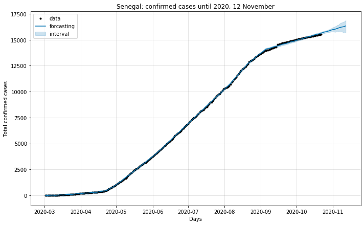
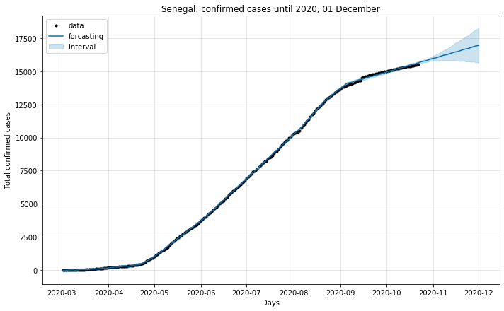
With Prophet, at November 12, 2020 we may obtain 16330 confirmed cases and 16950 confirmed cases at December 01, 2020 (see Tables 5 and 6, respectively). The forecastes of confirmed cases are illustrated in Figures 15a and 15b.

| ds | |||
|---|---|---|---|
| 2020-11-08 | 16213.793455 | 15776.476419 | 16625.216492 |
| 2020-11-09 | 16237.542798 | 15730.499926 | 16673.834380 |
| 2020-11-10 | 16254.670226 | 15734.183777 | 16750.503940 |
| 2020-11-11 | 16297.865380 | 15743.971264 | 16792.203760 |
| 2020-11-12 | 16335.788237 | 15755.096121 | 16875.197916 |

| ds | |||
|---|---|---|---|
| 2020-11-27 | 16841.363557 | 15724.240087 | 17997.233129 |
| 2020-11-28 | 16878.418793 | 15728.625383 | 18059.596350 |
| 2020-11-29 | 16911.177665 | 15665.479745 | 18162.293121 |
| 2020-11-30 | 16934.927009 | 15683.579005 | 18193.215306 |
| 2020-12-01 | 16952.054437 | 15654.901112 | 18268.706253 |
References
- [1] Agence Nationale de la Statistique et de la Démographie (ANSD), Senegal. Available online: https://www.ansd.sn (accessed on 26 September 2020).
- [2] B.M. Ndiaye, M.A.M.T. Balde, D. Seck, Visualization and machine learning for forecasting of COVID-19 in Senegal, arXiv:2008.03135 [q-bio.PE], 6 Aug 2020, https://arxiv.org/pdf/2008.03135.
- [3] M.A.M.T. Balde, C. Balde, B.M. Ndiaye, Impact studies of nationwide measures COVID-19 anti-pandemic: compartmental model and machine learning, arXiv:2005.08395 [q-bio.PE], 17 May 2020, https://arxiv.org/pdf/2005.08395.
- [4] M.A.M.T. Balde, Fitting SIR model to COVID-19 pandemic data and comparative forecasting with machine learning, medRxiv (2020). https://doi.org/10.1101/2020.04.26.20081042.
- [5] J.J. Cavallo, D.A. Donoho, H.P. Forman, Hospital Capacity and Operations in the Coronavirus Disease 2019 (COVID-19) Pandemic—Planning for the Nth Patient, JAMA Health Forum, Published online March 17, 2020. doi:10.1001/jamahealthforum.2020.0345.
- [6] M. Diaby, O. Diop, A. Konté, and A. Sène, A. COVID-19 Propagation Mathematical Modeling: The Case of Senegal. Preprints 2020, 2020060224 doi:10.20944/preprints202006.0224.v1.
- [7] R. Djidjou-Demasse, Y. Michalakis, M. Choisy, M. T. Sofonea, S. Alizon, Optimal COVID-19 epidemic control until vaccine deployment, medRxiv (2020). doi:https://doi.org/10.1101/2020.04.02.20049189.
- [8] IHME COVID-19 health service utilization forecasting team, C. J.L. Murray, Forecasting COVID-19 impact on hospital bed-days, ICU-days, ventilator-days and deaths by US state in the next 4 months, medRxiv (2020). doi:https://doi.org/10.1101/2020.03.27.20043752.
- [9] Z. Liu, P. Magal, O. Seydi, G. F. Webb, Understanding unreported cases in the 2019-nCov epidemic outbreak in Wuhan, China, and the importance of major health interventions, MPDI Biology (2020), 9, 50.
- [10] Z. Liu, P. Magal, O. Seydi, G. F. Webb, Predicting the cumulative number of cases for the COVID-19 in China from early data, Mathematical Biosciences and Engineering, 17(4), (2020), 3040-3051.
- [11] Z. Liu, P. Magal, O. Seydi, G. F. Webb, A COVID-19 epidemic model with latency period, Infectious Disease Modelling 5 (2020), 323-337.
- [12] Z. Liu, P. Magal, O. Seydi, G. F. Webb, A model to predict COVID-19 epidemics with applications to South Korea, Italia, and Spain, SIAM News, 53(4) (2020).
- [13] Ministre de la santé et de l’action sociale. Situation du Covid-19 au Sénégal. Available online: www.sante.gouv.sn/ (accessed on 26 September 2020).
- [14] S. M. Moghadas, et al., Projecting hospital utilization during the COVID-19 outbreaks in the United States, Proceedings of the National Academy of Sciences, 117(16), (2020), 9122-9126.
- [15] B.M. Ndiaye, L. Tendeng, D. Seck, Analysis of the COVID-19 pandemic by SIR model and machine learning technics for forecasting, arXiv:2004.01574 [q-bio.PE], 3 Apr 2020, https://arxiv.org/pdf/2004.01574.
- [16] B.M. Ndiaye, L. Tendeng, D. Seck, Comparative prediction of confirmed cases with COVID-19 pandemic by machine learning, deterministic and stochastic SIR models, arXiv:2004.13489 [q-bio.PE], 24 Apr 2020, https://arxiv.org/pdf/2004.13489.
- [17] V.M. Ndiaye, S.O. Sarr, B.M. Ndiaye, Impact of contamination factors on the COVID-19 evolution in Senegal, arXiv:2006.16326 [q-bio.PE], 29 Jun 2020, https://arxiv.org/pdf/2006.16326.
- [18] M. Samb, B.M. Ndiaye, Logistic growth model and modeling of factors for community case transmission, arXiv:2011.02766 [q-bio.PE], 5 Nov 2020, https://arxiv.org/pdf/2011.02766v1.
- [19] Prophet: Automatic Forecasting Procedure. Available online: https://facebook.github.io/prophet/docs/ or https://github.com/facebook/prophet (accessed on 26 September 2020).
- [20] Python Software Foundation. Python Language Reference, version 2.7. Available online: http://www.python.org (accessed on 26 September 2020).
- [21] Q. Richard, S. Alizon, M. Choisy, M. T. Sofonea, R. Djidjou-Demasse, Age-structured non-pharmaceutical interventions for optimal control of COVID-19 epidemic, medRxiv (2020). doi:https://doi.org/10.1101/2020.06.23.20138099.
- [22] S.J. Taylor, B. Letham, Forecasting at scale, PeerJ Preprints (2017) 5:e3190v2https://doi.org/10.7287/peerj.preprints.3190v2.
- [23] G. E. Weissman et al., Locally Informed Simulation to Predict Hospital Capacity Needs During the COVID-19 Pandemic, Annals of internal medicine, 173(1), (2020), 21-28.
- [24] Wikipedia, Template:COVID-19 pandemic data. Available online: https://en.wikipedia.org/wiki/Template:COVID-19_pandemic_data (accessed on 26 September 2020).
- [25] WHO Timeline–COVID-19. Available online: https://www.who.int/news-room/detail/27-04-2020-who-timeline---covid-19 (accessed on 26 September 2020).
- [26] World Health Organization. Pneumonia of Unknown Cause–China.Disease Outbreak News, 5 January 2020. Available online: https://www.who.int/csr/don/05-january-2020-pneumonia-of-unkown-cause-china/en/ (accessed on 26 September 2020).