Long-range phase order in two dimensions under shear flow

Abstract

We theoretically and numerically investigate a two-dimensional O(2) model where an order parameter is convected by shear flow. We show that a long-range phase order emerges in two dimensions as a result of anomalous suppression of phase fluctuations by the shear flow. Furthermore, we use the finite-size scaling theory to demonstrate that a phase transition to the long-range ordered state from the disordered state is second order. At a transition point far from equilibrium, the critical exponents turn out to be close to the mean-field value for equilibrium systems.

Introduction.— Nature exhibits various types of long-range order such as crystalline solids, liquid crystals, ferromagnets, and Bose–Einstein condensation. Whereas they are ubiquitous in the three-dimensional world, some types of long-range order associated with a continuous symmetry breaking are forbidden in two dimensions by the Mermin–Wagner theorem Mermin and Wagner (1966); Hohenberg (1967); Mermin (1968). The representative example of this theorem is that there is no long-range phase order in two dimensions.

Recently, the long-range phase order out of equilibrium has been attracted much attention. A stimulating example is the characteristic “flocking” behavior among living things such as birds and bacteria. According to extensive numerical simulations of a simple model proposed by Vicsek et al. Vicsek et al. (1995), the “flocking” behavior was identified with the spontaneous emergence of the phase order in self-propelled polar particle systems - it is often called the polar order Chaté (2020). A remarkable feature here is that it occurs even in two dimensions Toner and Tu (1995, 1998); Nishiguchi et al. (2017); Dadhichi et al. (2018); Tanida et al. (2020); Dadhichi et al. (2020), even though it is prohibited for equilibrium systems by the Mermin–Wagner theorem Tasaki . This phenomenon was also observed in the two-temperature conserved XY model Bassler and Rácz (1995); Reichl et al. (2010). It is now accepted that the long-range phase order can exist even in two dimensions for some non-equilibrium systems with short-range interactions.

The aim of this Letter is to clarify how the long-range phase order emerges in two dimensions under a small non-equilibrium perturbation to equilibrium systems. We study a two-dimensional O(2) model with short-range interaction. For equilibrium O(2) models, the dimension $d=2$ is marginal; specifically, the long-range phase order is broken by thermal fluctuations for $d\leq 2$, but is stable for $d>2$ Berezinskii (1971); Kosterlitz and Thouless (1973); Kosterlitz (1974); Koma and Tasaki (1995). Here, we impose infinitesimal shear flow on such a system and drive it into a non-equilibrium steady state. We then ask whether long-range phase order appears in the externally driven system. This Letter shows that the answer is yes and investigates its origin.

There is a long history of studying phase transitions driven by external non-equilibrium forces. Well-studied examples are related to the Ising universality class, such as critical fluids, binary mixtures and lattice gases Katz et al. (1984); van Beijeren and Schulman (1984); Wang et al. (1989); Leung (1991); Caracciolo et al. (2004); Marro and Dickman (2005). The phase transition under shear flow was one of the topic examined in this context Onuki and Kawasaki (1979); Onuki (1997, 2002); Corberi et al. (1999); Cirillo et al. (2005); Hucht (2009); Saracco and Gonnella (2009); Winter et al. (2010); Angst et al. (2012). As a seminal study, Onuki and Kawasaki performed the renormalization group analysis of the sheared critical fluids Onuki and Kawasaki (1979). Recently, some group studied the related systems by using Monte Carlo simulations Cirillo et al. (2005); Saracco and Gonnella (2009); Winter et al. (2010); Angst et al. (2012).

Regarding externally driven systems with continuous symmetry, the main focus has been on three-dimensional phenomena such as an isotropic-to-lamellar transition of block copolymer melts Cates and Milner (1989); Koppi et al. (1993); Fredrickson (1994); Zvelindovsky et al. (2000), an isotropic-to-nematic transition of liquid crystals Olmsted and Goldbart (1990, 1992); Grizzuti and Maffettone (2003); Lettinga and Dhont (2004); Hobbie and Fry (2006); Ripoll et al. (2008), an nematic-to-smectic transition of liquid crystals Gennes (1976); Bruinsma and Safinya (1991); Safinya et al. (1991), a crystallization of colloidal suspensions Butler and Harrowell (2002); Miyama and Sasa (2011), and a spinodal decomposition of a large-$N$ limit model Corberi et al. (2002, 2003). To our knowledge, the main question of this Letter has been never addressed before.

The key point of our study is to argue the stability of the long-range phase order in terms of the infrared divergence Goldenfeld (2018). For the equilibrium O(2) model, the correlation function of the phase fluctuation behaves as $|\bm{k}|^{-2}$ where $\bm{k}$ represents the wavenumber. This fluctuation causes the logarithmic divergence of the real-space correlation function in the limit of large system size, and breaks the ordered state. Therefore, if stable long-range phase order appears under the shear flow, this logarithmic divergence must be removed by the flow effects. In this Letter, we theoretically demonstrate that the shear flow anomalously suppresses the phase fluctuation from $k_{x}^{-2}$ to $|k_{x}|^{-2/3}$, where the $x$-direction is defined as parallel to the flow. This new phase fluctuation is small enough to remove the divergence. Furthermore, by performing finite-size scaling analysis, we numerically show that the phase transition to the ordered state from the disordered state is second order. We also discuss our simulation result in the context of the previous results obtained for the sheared Ising model.

Model.— Let $\bm{\varphi}(\bm{r},t)=(\varphi_{1}(\bm{r},t),\varphi_{2}(\bm{r},t))$ be a two-component real order parameter defined on a two-dimensional region $[0,L_{x}]\times[0,L_{y}]$. The order parameter is convected by the steady uniform shear flow with a velocity $\bm{v}(\bm{r})=(\dot{\gamma}y,0)$, where $\dot{\gamma}\geq 0$ without loss of generality. The dynamics is given by the time-dependent Ginzburg–Landau model:

$$\Big{[}\frac{\partial}{\partial t}+\bm{v}\cdot\nabla\Big{]}\varphi_{a} = -\Gamma\frac{\delta\Phi[\bm{\varphi}]}{\delta\varphi_{a}}+\eta_{a},$$ (1)

$$\langle\eta_{a}(t,\bm{r})\eta_{b}(t^{\prime},\bm{r}^{\prime})\rangle = 2\Gamma T\delta_{ab}\delta(t-t^{\prime})\delta(\bm{r}-\bm{r}^{\prime}),$$ (2)

where the Landau free energy $\Phi[\bm{\varphi}]$ is given by the standard $\varphi^{4}$ model

$$\Phi[\bm{\varphi}]=\int d^{2}\bm{r}\Big{[}\frac{\kappa}{2}\sum_{a=1}^{2}(\nabla\varphi_{a})^{2}+\frac{r}{2}|\bm{\varphi}|^{2}+\frac{u}{4}(|\bm{\varphi}|^{2})^{2}\Big{]}.$$ (3)

Here, $T$ is the temperature of the thermal bath and it is chosen independently of $r$.

The left-hand side of Eq. (1) represents the rate of change following the flow. We stress that the convection term does not break the rotational symmetry in the order-parameter space. Furthermore, we note that in equilibrium our model is reduced to “model A” in the classification of Hohenberg and Halperin Hohenberg and Halperin (1977); Mazenko (2008). Because the steady-state distribution of $\bm{\varphi}$ is given by the canonical ensemble, the system exhibits quasi-long-range order instead of long-range order Kosterlitz and Thouless (1973); Gupta and Baillie (1992).

Phase fluctuation in the low-temperature limit.— The state realized at $T=0$ is given by minimizing the Landau free energy $\Phi[\bm{\varphi}]$. For $r<0$, we have the ordered solution $\bm{\bar{\varphi}}=(\sqrt{-r/u},0)$, where we choose the direction of ordering as $\bm{n}=(1,0)$. In equilibrium, this ordered state is broken at finite temperature $T>0$. Here, we study how the shear flow suppresses the equilibrium fluctuations and stabilizes the ordered state in the low-temperature limit.

To analyze the fluctuations around $\bm{\bar{\varphi}}$, we transform the field variable as $\bm{\varphi}(\bm{r},t)=(\sqrt{-r/u}+A(\bm{r},t))\big{(}\cos\theta(\bm{r},t),\sin\theta(\bm{r},t)\big{)}$, where $A(\bm{r},t)$ is the amplitude fluctuation and $\theta(\bm{r},t)$ the phase fluctuation. The phase fluctuation corresponds to the gapless mode associated with O(2) symmetry breaking Goldstone (1961); Nambu and Jona-Lasinio (1961); Goldstone et al. (1962). Therefore, we study the phase fluctuation below. Because the thermal fluctuations become sufficiently small in the low-temperature limit, we can neglect the periodicity of $\theta(\bm{r},t)$ and describe its dynamics within the linear approximation as

$$\Big{[}\frac{\partial}{\partial t}-\dot{\gamma}k_{x}\frac{\partial}{\partial k_{y}}+\Gamma\kappa|\bm{k}|^{2}\Big{]}\tilde{\theta}(\bm{k},t)=\tilde{\eta}_{2}(\bm{k},t),$$ (4)

where $\tilde{\theta}(\bm{k},t)$ is the Fourier transform of $\theta(\bm{r},t)$. The equal-time correlation function $C_{\theta\theta}(\bm{k})$ in the steady state is defined by $\big{\langle}\tilde{\theta}(\bm{k},t)\tilde{\theta}(\bm{k}^{\prime},t)\big{\rangle}=C_{\theta\theta}(\bm{k})\delta(\bm{k}+\bm{k}^{\prime})$, where $\langle\cdots\rangle$ represents the average in the steady state. From Eq. (4), $C_{\theta\theta}(\bm{k})$ is formally solved as 

$$C_{\theta\theta}(\bm{k})=T\Gamma\int_{0}^{\infty}dse^{-\Gamma\kappa\big{(}s|\bm{k}|^{2}+\frac{1}{2}\dot{\gamma}s^{2}k_{x}k_{y}+\frac{1}{12}\dot{\gamma}^{2}s^{3}k_{x}^{2}\big{)}}.$$ (5)

For $\dot{\gamma}=0$, Eq. (5) is immediately integrated as $C_{\theta\theta}(\bm{k})=T|\bm{k}|^{-2}/\kappa$. In two dimensions, the $|\bm{k}|^{-2}$ mode leads to the logarithmic divergence of the real-space correlation function and destroys the long-range order.

For $\dot{\gamma}>0$, the asymptotic behavior of Eq. (5) for small $\bm{k}$ is calculated as

$$C_{\theta\theta}(\bm{k})\simeq\frac{T}{c_{0}(\sqrt{\kappa}\dot{\gamma}|k_{x}|/\Gamma)^{{\frac{2}{3}}}+\kappa|\bm{k}|^{2}},$$ (6)

where $c_{0}\simeq 2.04$. The shear flow stretches the fluctuations along the $x$-axis, which induces the anisotropic term $(\sqrt{\kappa}\dot{\gamma}|k_{x}|/\Gamma)^{{\frac{2}{3}}}$ in Eq. (6). Because the exponent $2/3$ of this term is smaller than $2$, the equilibrium fluctuations are suppressed so that the logarithmic divergence in two dimensions is removed. Therefore, the fluctuations under shear flow do not break the long-range phase order for sufficiently low temperatures.

We also observe the exponent $2/3$ beyond the linear regime. To this end, we numerically solve the full equation (1) and calculate the structure factor, defined by $\langle\bm{\varphi}(\bm{k})\cdot\bm{\varphi}(\bm{k}^{\prime})\rangle=S(\bm{k})\delta(\bm{k}+\bm{k}^{\prime})$. Figure 1 plots $S^{-1}(\bm{k})$ for $\Gamma=T=u=1.0$, $\kappa=0.5$, $\dot{\gamma}=0.1$ and $r=-3.01$, where we have the long-range ordered state as explained below. From this figure, we find that the $k_{x}$-dependence of $S^{-1}(k_{x},k_{y}=0)$ crosses over from $|k_{x}|^{-2/3}$ to $k_{x}^{-2}$. This behavior qualitatively agrees with the linearized model, Eq. (6).

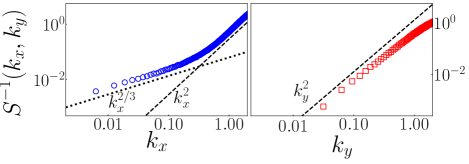
Figure 1: (Color online) Structure factor in ordered state. Left: $S^{-1}(k_{x},k_{y}=0)$ versus $k_{x}$. Right: $S^{-1}(k_{x}=0,k_{y})$ versus $k_{y}$.

We note that the length scale $l\equiv\sqrt{\kappa\Gamma/\dot{\gamma}}$ governs the crossover behavior. Because $l\to\infty$ in the equilibrium limit $\dot{\gamma}\to+0$, the order of the two limits $\bm{k}\to\bm{0}$ and $\dot{\gamma}\to+0$ cannot be exchanged. This observation leads to the result that the fractional mode $|k_{x}|^{-2/3}$ stabilizes the long-range order even when $\dot{\gamma}\to+0$.

Finite-size scaling analysis.— We carry out finite-size scaling analysis to show further evidences of long-range order in the presence of shear flow. Because the finite-size scaling theory in isotropic systems is modified by the anisotropy of shear flow Winter et al. (2010), we give an overview below of the finite-size scaling theory in the sheared system. Essentially the same analysis has been used for driven lattice gases Binder and Wang (1989); Wang et al. (1989); Leung (1991); Caracciolo et al. (2004).

The finite-size scaling theory is constructed on the basis of the scaling invariance at the second-order phase transition point. The scaling invariance is mathematically expressed by two relations. The first one is written using a free energy $F(\tau,h,L^{-1}_{x},L^{-1}_{y};\dot{\gamma})$ in the finite-size system, where $\tau=(r-r_{c})/r_{c}$ is the dimensionless distance from the transition point $r_{c}$, and $h$ is the external field coupled with $\hat{m}=|\int d^{2}\bm{r}\bm{\varphi}(\bm{r})|/L_{x}L_{y}$. Then, the scaling invariance of the free energy near the critical point is given by the scaling relation

$$F(\tau,h,L^{-1}_{x},L^{-1}_{y};\dot{\gamma})=F(b^{z_{\tau}}\tau,b^{z_{h}}h,b^{z_{x}}L^{-1}_{x},bL^{-1}_{y};\dot{\gamma})$$ (7)

for any $b>0$, where the three scaling dimensions $z_{\tau}$, $z_{h}$, and $z_{x}$ are introduced. The second relation is that any quantity $\langle A\rangle_{h=0}$ in the absence of an external field can be expressed in terms of the correlation lengths $\xi_{x}$ and $\xi_{y}$ as

$$\langle A\rangle_{h=0}(L^{-1}_{x},L^{-1}_{y},\tau;\dot{\gamma})=L_{x}^{w_{A}}\mathcal{A}\Big{(}\frac{\xi_{x}}{L_{x}},\frac{\xi_{y}}{L_{y}};\dot{\gamma}\Big{)},$$ (8)

where $w_{A}$ is a constant and $\mathcal{A}$ is a scaling function.

All the critical exponents are expressed by combinations of the three scaling dimensions $z_{\tau}$, $z_{h}$, and $z_{x}$ . For example, the critical exponents $\nu_{x}$ and $\nu_{y}$, characterizing the divergence of the correlation length (i.e. $\xi_{i}\sim|\tau|^{-\nu_{i}}$), are expressed as $\nu_{x}=z_{x}/z_{\tau}$ and $\nu_{y}=1/z_{\tau}$. The exponent $\beta$, characterizing the onset of magnetization slightly below the critical point (i.e. $\langle\hat{m}\rangle_{h=0}\sim|\tau|^{\beta}$), is given by $\beta=-\tilde{z}_{h}/z_{\tau}$, where we have introduced $\tilde{z}_{h}\equiv z_{h}-(1+z_{x})$.

We note that $z_{x}$ characterizes the anisotropy of the divergence of the correlation length because it is rewritten as $\nu_{x}/\nu_{y}$. Actually, the anisotropy of the shear flow makes $z_{x}\neq 1$. This can be immediately confirmed from the theoretical analysis of the linearized model by dropping the $\varphi^{4}$ term from Eq. (3). This model is well-defined for $r>0$ and exhibits a singular divergence as $r\to+0$. From a similar calculation as the phase fluctuations in the low-temperature limit, we obtain $\nu_{x}=3/2$ and $\nu_{y}=1/2$, and then $z_{x}$ is given by $z_{x}=\nu_{x}/\nu_{y}=3$. Thus, it is natural to introduce $z_{x}\neq 1$ in the presence of the shear flow.

Now, we show that the finite-size scaling theory works well for our model using numerical simulations. Below, we fix $\Gamma=T=u=1.0$ and $\kappa=0.5$, and treat $\dot{\gamma}$ and $r$ as control parameters. From Eqs. (7) and (8), we can derive the system-size dependence of the $n$-th moment of magnetization as

$$\big{\langle}\hat{m}^{n}\big{\rangle}_{h=0}(L^{-1}_{x},L^{-1}_{y},\tau;\dot{\gamma})=L_{y}^{\tilde{z}_{h}n}\mathcal{M}_{n}(L_{y}^{z_{\tau}}\tau,L_{y}^{z_{x}}L^{-1}_{x};\dot{\gamma}).$$ (9)

The Binder parameter, defined by $U\equiv\big{\langle}\hat{m}^{4}\big{\rangle}_{h=0}/\big{\langle}\hat{m}^{2}\big{\rangle}_{h=0}^{2}$, satisfies

$$U(L^{-1}_{x},L^{-1}_{y},{\tau};\dot{\gamma})=\mathcal{U}(L_{y}^{z_{\tau}}\tau,L_{y}^{z_{x}}L^{-1}_{x};\dot{\gamma}).$$ (10)

This equation means that all curves of the Binder parameter with different $L_{x}$ values intersect at a unique point when $L_{y}^{z_{x}}L^{-1}_{x}$ is fixed. In Fig. 2, we plot the numerical result for the Binder parameter $U$ for $\dot{\gamma}=5.0$. We have assumed $z_{x}=3$ with reference to the linearized model and chosen the system size as $L_{x}=125$, $216$, $343$, and $512$ under the condition $L_{y}=20L_{x}^{1/3}$. This figure shows the existence of the unique intersection point as expected.

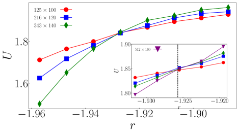
Figure 2: (Color online) Binder parameter $U$ as a function of $r$ for $\dot{\gamma}=5.0$. Inset: zoom of the intersection point. The error bars of the data are in the order of the point sizes.

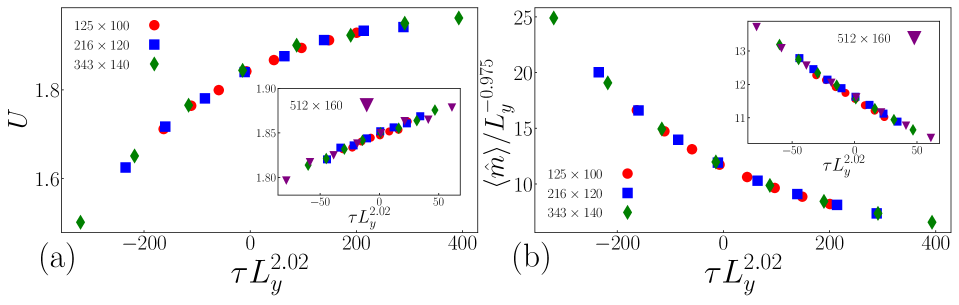
Figure 3: (Color online) Finite-size scaling plot for $\dot{\gamma}=5.0$. (a): $U$ versus $\tau L_{y}^{z_{\tau}}$. (b) $\big{\langle}\hat{m}\big{\rangle}_{h=0}/L^{\tilde{z}_{h}}_{y}$ versus $\tau L_{y}^{z_{\tau}}$. In both figures, the inset is an enlargement of $\tau=0$. $r_{c}$, $z_{\tau}$ and $\tilde{z}_{h}$ are fixed at the best-fit value. The error bars of the data are in the order of the point sizes.

According to the finite-size scaling relations Eqs. (9) and (10), the magnetization $\big{\langle}\hat{m}\big{\rangle}_{h=0}$ and the Binder parameter $U$ can be expanded as power series near the critical point:

$$\big{\langle}\hat{m}\big{\rangle}_{h=0} = L_{y}^{\tilde{z}_{h}}\sum_{n=0}^{N}C^{m}_{n}(L_{y}^{z_{x}}L^{-1}_{x})L_{y}^{z_{\tau}n}\tau^{n},$$ (11)

$$U = \sum_{n=0}^{N}C^{u}_{n}(L_{y}^{z_{x}}L^{-1}_{x})L_{y}^{z_{\tau}n}\tau^{n},$$ (12)

where $C^{m}_{n}$ and $C^{u}_{n}$ are expansion coefficients dependent on $L_{y}^{z_{x}}L^{-1}_{x}$. By fitting the simulation data to these expansions, we determine the critical point $r_{c}$ and the scaling exponent $(\tilde{z}_{h},z_{\tau})$. In particular, we use the data in the region $-1.930<r<-1.920$ and perform simultaneous fitting of the two quantities $\big{\langle}\hat{m}\big{\rangle}_{h=0}$ and $U$ to Eqs. (11) and (12) with $N=2$; we obtain $r_{c}=-1.9257\pm 0.0002$, $z_{\tau}=2.05\pm 0.11$, and $\tilde{z}_{h}=-0.983\pm 0.026$. The validity of these fittings is shown in Fig. 3, which is the scaled plot of the two quantities $\big{\langle}\hat{m}\big{\rangle}_{h=0}$ and $U$. The scaled data for the different system sizes overlap, verifying the finite-size scaling relations Eqs. (11) and (12). It is noteworthy that the existence of the universal curve provides an evidence of $z_{x}=3$. We can also perform the consistency check of $z_{x}=3$ from the observation of $\nu_{x}$ and $\nu_{y}$ by using the property that $z_{x}$ is related to the anisotropy of the divergence of the correlation length .

From the obtained values of $z_{\tau}$ and $\tilde{z}_{h}$, the critical exponent $\beta$ is calculated as $\beta=-\tilde{z}_{h}/z_{\tau}=0.480\pm 0.029$. This behavior is very similar to the result for the mean-field theory of the $\varphi^{4}$ model in equilibrium. It is consistent with the previous theoretical results for the sheared Ising model Onuki and Kawasaki (1979); Hucht (2009), where the mean-field character is recovered under a sufficiently large shear rate or in the large limit.

Phase diagram.—

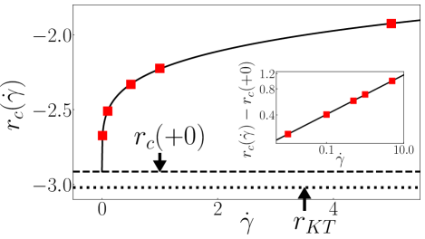
Figure 4: (Color online) Critical point $r_{c}$ as a function of $\dot{\gamma}$. The red points represent the numerical estimation and the black solid line Eq. (13) with the best-fit parameter. Inset: $r_{c}-r_{c}(+0)$ versus $\dot{\gamma}$ with a log-log plot.

We apply the above procedure to systems with smaller $\dot{\gamma}$ and show the phase diagram in Fig. 4, where the critical point $r_{c}$ is plotted as a function of $\dot{\gamma}$. For all $\dot{\gamma}$ values we have examined, the assumption $z_{x}=3$ is valid and the long-range phase order exists below $r_{c}$. We then ask where $r_{c}(\dot{\gamma})$ terminates as $\dot{\gamma}\to+0$. To answer this question, we assume that the critical point $r_{c}$ behaves as a function of $\dot{\gamma}$ in the form

$$r_{c}(\dot{\gamma})=D_{0}\dot{\gamma}^{w}+r_{c}(+0).$$ (13)

Note that for the sheared Ising model, this functional form is known to reproduce the behavior of the critical point for small $\dot{\gamma}$ Onuki (2002); Saracco and Gonnella (2009); Winter et al. (2010); Angst et al. (2012). By fitting the simulation data to Eq. (13), we obtain the best-fit parameters $r_{c}(+0)=-2.9139\pm 0.0151$, $D_{0}=0.685\pm 0.016$, and $w=0.228\pm 0.006$. The corresponding curve is drawn as the black solid one in Fig. 4. The good agreement between the numerical estimation and the best-fit curve confirms the validity of Eq. (13) for our model. This gives the evidence that the long-range phase order is stabilized even under the infinitesimal shear flow. The critical point at the infinitesimal shear rate $\dot{\gamma}\to+0$ is estimated as $r_{c}(+0)=-2.9139\pm 0.0151$.

Discussion.— We remember that our model exhibits the Kosterlitz–Thouless transition in equilibrium. The transition point is estimated to be $r_{KT}=-3.0204\pm 0.0087$ . Then, our results show that there exists a slight deviation between $r_{c}(+0)$ and $r_{KT}$. We here discuss two possible scenarios. The first one is that this deviation disappears by using the data at smaller $\dot{\gamma}$ for larger systems. Actually, for the two-dimensional Ising model Saracco and Gonnella (2009); Winter et al. (2010) and the three-dimensional critical fluid Onuki (2002), $r_{c}(\dot{\gamma})$ terminates at the equilibrium transition point as $\dot{\gamma}\to+0$. As the second scenario, this deviation may remains for larger systems because the long-wavelength fluctuations ($|k_{x}|<2\pi/l$) are drastically altered even when $\dot{\gamma}\to+0$ (See Fig. 1). Which scenario is correct is left for future study.

Another question for small $\dot{\gamma}$ is about the critical exponent $\beta$. Our simulation showed that for $\dot{\gamma}=0.5$, $\beta$ agrees well with the mean-field value as in the case of $\dot{\gamma}=5.0$. In contrast, for $\dot{\gamma}=0.01$, we obtained $z_{\tau}=2.03\pm 0.30$ and $\tilde{z}_{h}=-0.579\pm 0.02$, which corresponds to $\beta=0.285$ . Clearly, there is a large deviation between the observed result and mean-field theory. We do not judge whether this deviation comes from the finite-size effects or remains in the large system-size limit. On a related note, this problem also remains controversial for the sheared Ising model Hucht (2009); Saracco and Gonnella (2009); Winter et al. (2010); Angst et al. (2012). More careful analysis for smaller $\dot{\gamma}$ is necessary.

The phase mode induced by the shear flow, $S(k_{x},k_{y}=0)\sim|k_{x}|^{-2/3}$, and the long-range order are two sides of the same coin. The interesting point is that the exponent $2/3$ is numerically observed for all $\dot{\gamma}$ values we have examined, although it is derived without considering the nonlinear interaction of fluctuations. This observation suggests that nonlinear effects are irrelevant for the structure factor in the ordered state. The theoretical verification of this conjecture is left as a future work.

Finally, we discuss possible experiments associated with our result. The model in this Letter gives an ideal description of some experimental systems using liquid undercooled metals Reske et al. (1995); Albrecht et al. (1997) and magnetic fluids Nijmeijer and Weis (1995). The liquid undercooled metal is known to exhibit the liquid ferromagnet phase due to short-ranged exchange interactions in three dimensions Reske et al. (1995); Albrecht et al. (1997). We expect that the two-dimensional liquid ferromagnet phase can be observed by designing a two-dimensional system Nishiguchi et al. (2017).

Acknowledgements.— We thank M. Kobayashi for helpful comments on the numerical simulation, D. Nishiguchi for a critical reading of the manuscript, and M. Hongo for stimulating conversations. HN and SS are supported by KAKENHI (Nos. 17H01148, 19H05795, and 20K20425). YM is supported by the Zhejiang Provincial Natural Science Foundation Key Project (Grant No. LZ19A050001) and NSF of China (Grants No. 11975199 and 11674283).

S1 Linear analysis of fluctuations

We present the details of the linear analysis of fluctuations for the model Eqs. (1), (2), and (3). We first derive, in Sec. S1.1, the exact integral expression of correlation functions such as Eq. (5). Next, in Sec. S1.2, by using this expression, we perform the asymptotic analysis of fluctuations near the critical point. This result is applied to estimate the value of $z_{x}$ in the main text. Finally, in Sec. S1.3, we analyze linear fluctuations around the ordered solution. We also give the detail of derivation of Eq. (6).

S1.1 Formal solution of linearized model

The linearized model is obtained by dropping the non-linear term from Eqs. (1), (2), and (3) as

$$\frac{\partial\varphi_{a}}{\partial t}+\dot{\gamma}y\frac{\partial\varphi_{a}}{\partial x} = -\Gamma\Big{(}-\kappa\Delta+r\Big{)}\varphi_{a}+\eta_{a}.$$ (S1)

By the Fourier transform

$$\tilde{\varphi}_{a}(\bm{k})\equiv\int d^{2}\bm{r}\varphi_{a}(\bm{r})e^{i\bm{k}\cdot\bm{r}},$$ (S2)

Eq. (S1) is rewritten as

$$\frac{\partial\tilde{\varphi}_{a}}{\partial t}-\dot{\gamma}k_{x}\frac{\partial\tilde{\varphi}_{a}}{\partial k_{y}} = -\Gamma\Big{(}\kappa|\bm{k}|^{2}+r\Big{)}\tilde{\varphi}_{a}+\tilde{\eta}_{a}.$$ (S3)

In this subsection, we calculate $C_{\varphi\varphi}(\bm{k},t)$ defined by $\langle\tilde{\varphi}_{a}(\bm{k},t)\tilde{\varphi}_{b}(\bm{k}^{\prime},t)\rangle=C_{\varphi\varphi}(\bm{k},t)\delta_{ab}\delta(\bm{k}+\bm{k}^{\prime})$. Our argument is essentially the same as that by Onuki and Kawasaki Onuki and Kawasaki (1979).

We first derive the equation for $C_{\varphi\varphi}(\bm{k},t)$. Multiplying Eq. (S3) by $\tilde{\varphi}_{b}(\bm{k}^{\prime},t)$ yields

$$\tilde{\varphi}_{b}(\bm{k}^{\prime},t)\frac{\partial}{\partial t}\tilde{\varphi}_{a}(\bm{k},t)+\Big{(}-\dot{\gamma}k_{x}\frac{\partial}{\partial k_{y}}+\Gamma\big{(}\kappa|\bm{k}|^{2}+r\big{)}\Big{)}\tilde{\varphi}_{a}(\bm{k},t)\tilde{\varphi}_{b}(\bm{k}^{\prime},t)=\tilde{\eta}_{a}(\bm{k},t)\tilde{\varphi}_{b}(\bm{k}^{\prime},t).$$ (S4)

By taking the average over the noise, we have

$$\Big{\langle}\tilde{\varphi}_{b}(\bm{k}^{\prime},t)\frac{\partial}{\partial t}\tilde{\varphi}_{a}(\bm{k},t)\Big{\rangle}+\Big{(}-\dot{\gamma}k_{x}\frac{\partial}{\partial k_{y}}+\Gamma\big{(}\kappa|\bm{k}|^{2}+r\big{)}\Big{)}\Big{\langle}\tilde{\varphi}_{a}(\bm{k},t)\tilde{\varphi}_{b}(\bm{k}^{\prime},t)\Big{\rangle}=\Big{\langle}\tilde{\eta}_{a}(\bm{k},t)\tilde{\varphi}_{b}(\bm{k}^{\prime},t)\Big{\rangle}.$$ (S5)

Because $\big{\langle}\tilde{\eta}(\bm{k},t)\tilde{\varphi}_{a}(\bm{k}^{\prime},t)\big{\rangle}$ is defined by the Stratonovich convention, we have

$$\big{\langle}\tilde{\eta}_{a}(\bm{k},t)\tilde{\varphi}_{b}(\bm{k}^{\prime},t)\big{\rangle}=T\Gamma\delta_{ab}\delta(\bm{k}+\bm{k}^{\prime}),$$ (S6)

where $\delta(\bm{k})$ is the delta function with argument $\bm{k}$, and Eq. (S5) is rewritten as

$$\Big{\langle}\tilde{\varphi}_{b}(\bm{k}^{\prime},t)\frac{\partial}{\partial t}\tilde{\varphi}_{a}(\bm{k},t)\Big{\rangle}+\Big{(}-\dot{\gamma}k_{x}\frac{\partial}{\partial k_{y}}+\Gamma\big{(}\kappa|\bm{k}|^{2}+r\big{)}\Big{)}\Big{\langle}\tilde{\varphi}_{a}(\bm{k},t)\tilde{\varphi}_{b}(\bm{k}^{\prime},t)\Big{\rangle}=T\Gamma\delta_{ab}\delta(\bm{k}+\bm{k}^{\prime}).$$ (S7)

Here, by definition, the time derivative of $C_{\varphi\varphi}(\bm{k},t)$ satisfies the following equation:

$$\Big{\langle}\tilde{\varphi}_{a}(\bm{k},t)\frac{\partial\tilde{\varphi}_{b}(\bm{k}^{\prime},t)}{\partial t}\Big{\rangle}+\Big{\langle}\frac{\partial\tilde{\varphi}_{a}(\bm{k},t)}{\partial t}\tilde{\varphi}_{b}(\bm{k}^{\prime},t)\Big{\rangle}=\frac{\partial C_{\varphi\varphi}(\bm{k},t)}{\partial t}\delta_{ab}\delta(\bm{k}+\bm{k}^{\prime}).$$ (S8)

By substituting Eq. (S7) into Eq. (S8), we obtain

$$\frac{\partial C_{\varphi\varphi}(\bm{k},t)}{\partial t}=\Big{(}\dot{\gamma}k_{x}\frac{\partial}{\partial k_{y}}-2\Gamma\big{(}\kappa|\bm{k}|^{2}+r\big{)}\Big{)}C_{\varphi\varphi}(\bm{k},t)+2T\Gamma.$$ (S9)

This equation describes the time evolution of $C_{\varphi\varphi}(\bm{k},t)$. Because we are especially interested in the steady-state correlation, we set the time derivative of Eq. (S9) to zero and study the equation

$$\Big{(}-\frac{1}{2}\dot{\gamma}k_{x}\frac{\partial}{\partial k_{y}}+\Gamma\big{(}\kappa|\bm{k}|^{2}+r\big{)}\Big{)}C_{\varphi\varphi}(\bm{k})=T\Gamma,$$ (S10)

where $C_{\varphi\varphi}(\bm{k})$ is the steady state correlation defined by $C_{\varphi\varphi}(\bm{k})\equiv\lim_{t\to\infty}C_{\varphi\varphi}(\bm{k},t)$.

In equilibrium, Eq. (S10) takes the simple form

$$\Gamma\big{(}\kappa|\bm{k}|^{2}+r\big{)}C_{\varphi\varphi}(\bm{k})=T\Gamma,$$ (S11)

and we immediately find that $C_{\varphi\varphi}(\bm{k})$ is expressed as

$$C_{\varphi\varphi}(\bm{k})=\frac{T}{\kappa|\bm{k}|^{2}+r}.$$ (S12)

For $\dot{\gamma}\neq 0$, although the first term of Eq. (S10) is the differential operator, we can write $C_{\varphi\varphi}(\bm{k})$ as

$$C_{\varphi\varphi}(\bm{k})=\frac{\Gamma T}{-\frac{1}{2}\dot{\gamma}k_{x}\frac{\partial}{\partial k_{y}}+\Gamma\big{(}\kappa|\bm{k}|^{2}+r\big{)}}.$$ (S13)

The inverse operator of Eq. (S13) is expressed as

$$\frac{1}{-\frac{1}{2}\dot{\gamma}k_{x}\frac{\partial}{\partial k_{y}}+\Gamma\big{(}\kappa|\bm{k}|^{2}+r\big{)}}=\int_{0}^{\infty}dse^{-s\big{\{}-\frac{1}{2}\dot{\gamma}k_{x}\frac{\partial}{\partial k_{y}}+\Gamma(\kappa|\bm{k}|^{2}+r)\big{\}}}.$$ (S14)

Here, it is known that the exponential operator containing the first-order differential is decomposed as

$$e^{\lambda U(x)+\lambda\frac{\partial}{\partial x}}=e^{\int_{0}^{\lambda}d\lambda^{\prime}U(x+\lambda^{\prime})}e^{\lambda\frac{\partial}{\partial x}}.$$ (S15)

We will give a proof of this formula later. By applying this formula to Eq. (S14) and substituting it into Eq. (S13), we obtain

$$C_{\varphi\varphi}(\bm{k})=T\Gamma\int_{0}^{\infty}dse^{-\int_{0}^{s}d\lambda\Gamma(\kappa|\bm{\kappa}_{\lambda}|^{2}+r)}$$ (S16)

with

$$\bm{\kappa}_{\lambda}=(k_{x},k_{y}+\frac{1}{2}\dot{\gamma}\lambda k_{x}).$$ (S17)

The $\lambda$-integral in Eq. (S16) is straightforwardly calculated as

$$C_{\varphi\varphi}(\bm{k})=T\Gamma\int_{0}^{\infty}dse^{-\Gamma\big{\{}s(\kappa|\bm{k}|^{2}+r)+\frac{1}{2}\kappa\dot{\gamma}s^{2}k_{x}k_{y}+\frac{1}{12}\kappa\dot{\gamma}^{2}s^{3}k_{x}^{2}\big{\}}}.$$ (S18)

This is the desired expression for the correlation function under shear flow. This type of expression was firstly derived by Onuki and Kawasaki Onuki and Kawasaki (1979) and widely used in the analyses of fluctuations in the presence of shear flow Gennes (1976); Fredrickson (1986); Cates and Milner (1989); Corberi et al. (2002, 2003); Wada and Sasa (2003); Wada (2004); Otsuki and Hayakawa (2009).

Derivation of Eq. (S15)

We here give a proof of the formula Eq. (S15). We define two functions by

$$g(x,\lambda)\equiv e^{\lambda U(x)+\lambda\frac{\partial}{\partial x}}f(x),$$ (S19)

$$h(x,y)\equiv g(x,y-x)$$ (S20)

for any function $f(x)$. Noting

$$\frac{\partial g(x,\lambda)}{\partial\lambda}=U(x)g(x,\lambda)+\frac{\partial g(x,\lambda)}{\partial x},$$ (S21)

we calculate the $x$-differential of $h(x,y)$ as

$$\frac{\partial h(x,y)}{\partial x}=-U(x)h(x,y).$$ (S22)

Then, by integrating with respect to $x$, we obtain

$$h(x,y) = h(y,y)e^{-\int_{y}^{x}dsU(s)}$$ (S23)

$$= h(y,y)e^{\int_{0}^{y-x}dsU(y-s)}.$$

This leads to

$$g(x,\lambda) = h(x,x+\lambda)$$ (S24)

$$= h(x+\lambda,x+\lambda)e^{\int_{0}^{\lambda}dsU(x+\lambda-s)}$$

$$= g(x+\lambda,0)e^{\int_{0}^{\lambda}d\lambda^{\prime}U(x+\lambda^{\prime})}.$$

Because $e^{\lambda\frac{\partial}{\partial x}}$ is the translational operator, we have

$$g(x+\lambda,0)=f(x+\lambda)=e^{\lambda\frac{\partial}{\partial x}}f(x).$$ (S25)

By combining Eqs. (S24) and (S25), we obtain the desired identity

$$e^{\lambda U(x)+\lambda\frac{\partial}{\partial x}}f(x)=e^{\int_{0}^{\lambda}d\lambda^{\prime}U(x+\lambda^{\prime})}e^{\lambda\frac{\partial}{\partial x}}f(x).$$ (S26)

S1.2 Fluctuations near the critical point

The linearized model (S1) or (S3) is valid for $r>0$, and exhibits a singular behavior as $r\to+0$. This singular behavior is characterized by the divergence of the correlation length. As the simplest example, let us consider the case $k_{x}=0$. In this case, we immediately calculate the $s$-integral in (S18) for any $r$ and obtain

$$C_{\varphi\varphi}(k_{x}=0,k_{y})=\frac{T}{r+\kappa k_{y}^{2}}.$$ (S27)

Then, we find that the correlation length $\xi_{y}$ diverges as

$$\xi_{y}\sim r^{-1/2}$$ (S28)

as $r\to+0$. Except for the simple wavelength region, we cannot perform the $s$-integral in (S18). Then, we focus on the asymptotic behavior of $C_{\varphi\varphi}(\bm{k})$ in the long-wavelength region and argue how the correlation length diverges. Below, $r$ is assumed to be sufficiently small.

We study two limiting $\bm{k}$-regions:

$${\rm(i)}\ \ \frac{1}{12}\dot{\gamma}^{2}k_{x}^{2}\ll\Gamma^{2}\big{(}\kappa|\bm{k}|^{2}+r\big{)}^{3},$$ (S29)

$${\rm(ii)}\ \ \frac{1}{12}\dot{\gamma}^{2}k_{x}^{2}\gg\Gamma^{2}\big{(}\kappa|\bm{k}|^{2}+r\big{)}^{3}.$$ (S30)

The schematic image of each region is drawn in Fig. S1. Naively speaking, region (i) is located near $k_{x}=0$, and region (ii) corresponds to all other region.

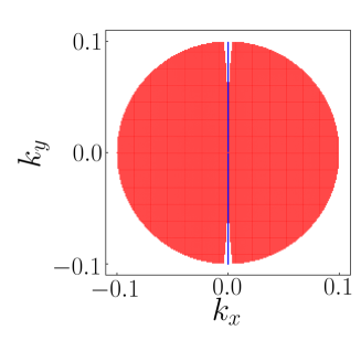
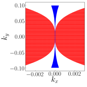
Figure S1: (Color online) Schematic image of two regions (i) and (ii) for $\dot{\gamma}=\Gamma=1.0$, $\kappa=0.5$ and $r=0$. The blue and red regions, respectively, represent region (i) and (ii). The right side is the zoom of $k_{x}=0$.

In region (i), the dominant contribution of the $s$-integral in Eq. (S18) comes from near

$$s=\frac{1}{\Gamma(\kappa|\bm{k}|^{2}+r)},$$ (S31)

where the integrand is approximated as

$$e^{-\Gamma\big{\{}s(\kappa|\bm{k}|^{2}+r)+\frac{1}{2}\kappa\dot{\gamma}s^{2}k_{x}k_{y}+\frac{1}{12}\kappa\dot{\gamma}^{2}s^{3}k_{x}^{2}\big{\}}}\approx e^{-\Gamma s(\kappa|\bm{k}|^{2}+r)}.$$ (S32)

Then, Eq. (S18) is approximately integrated as

$$C_{\varphi\varphi}(\bm{k}) \simeq T\Gamma\int_{0}^{\infty}dse^{-\Gamma s(\kappa|\bm{k}|^{2}+r)}$$ (S33)

$$= \frac{T}{\kappa|\bm{k}|^{2}+r}.$$

Similarly, in region (ii), because the dominant contribution of the $s$-integral of Eq. (S18) comes from near

$$s=\Big{(}\frac{12}{\Gamma\kappa\dot{\gamma}^{2}k_{x}^{2}}\Big{)}^{\frac{1}{3}},$$ (S34)

$C_{\varphi\varphi}(\bm{k})$ is approximated as

$$C_{\varphi\varphi}(\bm{k}) \simeq T\Gamma\int_{0}^{\infty}dse^{-\frac{1}{12}\Gamma\kappa\dot{\gamma}^{2}s^{3}k_{x}^{2}}$$ (S35)

$$= \frac{12^{\frac{1}{3}}\Gamma(\frac{4}{3})T\Gamma^{\frac{2}{3}}}{\kappa^{\frac{1}{3}}\dot{\gamma}^{\frac{2}{3}}|k_{x}|^{\frac{2}{3}}},$$

where $\Gamma(x)$ is the Gamma function.

We here notice that the behavior of Eqs. (S33) and (S35) is obtained from the limiting case of the following expression

$$C_{\varphi\varphi}(\bm{k})=\frac{T}{r+\kappa|\bm{k}|^{2}+c_{0}(\Gamma^{-1}\sqrt{\kappa}\dot{\gamma}|k_{x}|)^{{\frac{2}{3}}}},$$ (S36)

where $c_{0}=12^{\frac{1}{3}}\Gamma(\frac{4}{3})\simeq 2.04$. This expression describes well the behavior of $C_{\varphi\varphi}(\bm{k})$ in the colored regions of Fig. S1. From this expression, we find that the correlation length diverges as

$$\xi_{x}\sim r^{-3/2}\ \ {\rm and}\ \ \xi_{y}\sim r^{-1/2}.$$ (S37)

S1.3 Fluctuations around the ordered solution

Next, we argue linear fluctuations around the ordered solution. For this purpose, we return to the model Eqs. (1), (2), and (3) and consider the regime $r<0$. As explained in the main text, it is useful to decompose the field variable $\bm{\varphi}(\bm{r},t)$ into

$$\bm{\varphi}(\bm{r},t)=\Big{(}\sqrt{-\frac{r}{u}}+A(\bm{r},t)\Big{)}\big{(}\cos\theta(\bm{r},t),\sin\theta(\bm{r},t)\big{)}.$$ (S38)

$A(\bm{r},t)$ and $\theta(\bm{r},t)$, respectively, correspond to the amplitude fluctuation and the phase fluctuation around the state realized at $T=0$. By substituting Eq. (S38) into Eqs. (1), (2), and (3) and neglecting the non-linear terms, we obtain

$$\Big{[}\frac{\partial}{\partial t}-\dot{\gamma}k_{x}\frac{\partial}{\partial k_{y}}+\Gamma(\kappa|\bm{k}|^{2}+2|r|)\Big{]}\tilde{A}(\bm{k},t)=\tilde{\eta}_{1}(\bm{k},t),$$ (S39)

$$\Big{[}\frac{\partial}{\partial t}-\dot{\gamma}k_{x}\frac{\partial}{\partial k_{y}}+\Gamma\kappa|\bm{k}|^{2}\Big{]}\tilde{\theta}(\bm{k},t)=\tilde{\eta}_{2}(\bm{k},t).$$ (S40)

Since Eq. (S40) is equivalent to Eq. (S3) with $r=0$, we can repeat the previous argument in Secs. S1.1 and S1.2. The final expression is given by

$$C_{\theta\theta}(\bm{k})\simeq\frac{T}{c_{0}(\Gamma^{-1}\sqrt{\kappa}\dot{\gamma}k_{x})^{{\frac{2}{3}}}+\kappa|\bm{k}|^{2}}.$$ (S41)

This equation is Eq. (6) in the main text.

The amplitude correlation $C_{AA}(\bm{k})$, defined by $\langle\tilde{A}(\bm{k},t)\tilde{A}(\bm{k}^{\prime},t)\rangle=C_{AA}(\bm{k})\delta(\bm{k}+\bm{k}^{\prime})$, is also calculated as

$$C_{AA}(\bm{k})=T\Gamma\int_{0}^{\infty}dse^{-\Gamma\big{\{}s(\kappa|\bm{k}|^{2}+2|r|)+\frac{1}{2}\kappa\dot{\gamma}s^{2}k_{x}k_{y}+\frac{1}{12}\kappa\dot{\gamma}^{2}s^{3}k_{x}^{2}\big{\}}}.$$ (S42)

In the long-wavelength region, the main contribution of the $s$-integral arises from $s=1/(2\Gamma|r|)$. Because

$$2\Gamma s|r|\gg\Gamma s\kappa|\bm{k}|^{2},\ \frac{1}{2}\Gamma\kappa\dot{\gamma}s^{2}k_{x}k_{y},\ \frac{1}{12}\Gamma\kappa\dot{\gamma}^{2}s^{3}k_{x}^{2}$$ (S43)

holds near $s=1/(2\Gamma|r|)$, Eq. (S42) is expanded as

$$C_{AA}(\bm{k})=T\Gamma\int_{0}^{\infty}dse^{-2\Gamma s|r|}\Big{(}1-\Gamma s\kappa|\bm{k}|^{2}-\frac{\Gamma}{2}\kappa\dot{\gamma}s^{2}k_{x}k_{y}-\frac{\Gamma}{12}\kappa\dot{\gamma}^{2}s^{3}k_{x}^{2}+\cdots\Big{)}.$$ (S44)

Then, the $s$-integral is calculated as

$$C_{AA}(\bm{k})=\frac{T}{2|r|}-\frac{T\kappa}{4|r|^{2}}|\bm{k}|^{2}-\frac{\dot{\gamma}}{\Gamma}\frac{T\kappa}{8|r|^{3}}k_{x}k_{y}\cdots.$$ (S45)

Finally, to make it easier to see, we rewrite it in the Ornstein–Zernike form

$$C_{AA}(\bm{k})=\frac{T}{2|r|+\kappa|\bm{k}^{2}|+\dot{\gamma}\kappa k_{x}k_{y}/(2\Gamma|r|)+\cdots}.$$ (S46)

Eqs. (S41) and (S46) give all the behaviors of fluctuations in the ordered state. In the real space, Eq. (S41) yields the power-law decay of the fluctuation, whereas Eq. (S46) gives the exponential decay. This result reflects the gapless nature of the phase fluctuation. We also find that the fractional exponent is specific to the phase fluctuations. The shear flow makes the amplitude fluctuation anisotropic without affecting the exponent.

Physical interpretation of suppression due to shear flow

The shear flow induces stretching of fluctuations along the $x$-axis. This is the origin of anisotropy of the correlation function Eq. (S41). Here, let us physically estimate the decay rate originating from the stretching, which is denoted by $\lambda_{s}$. We fix the system size in the $y$-direction as $L_{y}$ and consider a fluctuation with $k_{x}$. Because the diffusion time in the $y$-direction is given by $L_{y}^{2}/\Gamma\kappa$, the stretching over the diffusion time is given by $\dot{\gamma}k_{x}L_{y}^{3}/(\Gamma\kappa)$. The decay rate $\lambda_{s}$ in the low temperature limit is then expressed as

$$\lambda_{s}=\frac{\Gamma\kappa}{L_{y}^{2}}f\left(\frac{\dot{\gamma}k_{x}L_{y}^{3}}{\Gamma\kappa}\right),$$ (S47)

where $f$ is a dimensionless function. Here, we reasonably assume that $\lambda_{s}$ is independent of $L_{y}$ in the limit $\dot{\gamma}k_{x}L_{y}^{3}/(\Gamma\kappa)\to 0$. Then, the decay rate becomes

$$\lambda_{s}\simeq\dot{\gamma}\left(k_{x}\sqrt{\frac{\Gamma\kappa}{\dot{\gamma}}}\right)^{2/3},$$ (S48)

which is so large that the fluctuation disappears faster than the diffusion process. As the result, the fluctuation of the order parameter along the $x$-axis is suppressed.

S2 Numerical implementation of uniform shear flow

We explain a numerical implementation of shear flow. The dynamics of the order parameter is given by Eqs. (1), (2), and (3), which are explicitly written as

$$\frac{\partial\varphi_{a}}{\partial t}+\dot{\gamma}y\frac{\partial\varphi_{a}}{\partial x} = -\Gamma\Big{(}-\kappa\Delta+r+u|\bm{\varphi}|^{2}\Big{)}\varphi_{a}+\eta_{a}.$$ (S49)

Numerically solving Eq. (S49) in the Cartecian coordinate system is difficult because the term $\dot{\gamma}y\frac{\partial\varphi_{a}}{\partial x}$ at $y=L_{y}$ becomes larger in proportion to $L_{y}$. This difficulty is removed by using a new coordinates system moving with velocity $-\bm{v}$, which was firstly proposed by Toh et al. Toh et al. (1991) and secondly by Onuki Onuki (1997). Here, we briefly review this method.

First, we introduce the new coordinate system $(\bm{r}^{\prime},t^{\prime})=(x^{\prime},y^{\prime},t^{\prime})$ defined by

$$x^{\prime}=x-\dot{\gamma}ty\ ,\ y^{\prime}=y\ ,\ t^{\prime}=t.$$ (S50)

The order parameter in this coordinate system is given by $\hat{\varphi}_{a}(\bm{r}^{\prime},t^{\prime})=\varphi_{a}(\bm{r},t)$. The dynamics of $\hat{\varphi}_{a}(\bm{r}^{\prime},t^{\prime})$ is then derived from Eq. (S49) as

$$\frac{\partial\hat{\varphi}_{a}}{\partial t^{\prime}} = -\Gamma\Big{(}-\kappa\Delta^{\prime}+r+u|\hat{\bm{\varphi}}|^{2}\Big{)}\hat{\varphi}_{a}+\hat{\eta}_{a}$$ (S51)

with

$$\Delta^{\prime}=\Big{(}\frac{\partial}{\partial x^{\prime}}\Big{)}^{2}+\Big{(}\frac{\partial}{\partial y^{\prime}}-\dot{\gamma}t\frac{\partial}{\partial x^{\prime}}\Big{)}^{2}.$$ (S52)

Eq. (S51) does not contain the term proportional to $y$, but instead contains the term proportional to $t$. For $0\leq t\leq 1/\dot{\gamma}$, this term is numerically stable because it remains $O(1)$. However, this term becomes so large for $t\gg 1/\dot{\gamma}$. In order to overcome this difficulty, we repeat the coordinate transformation at every $1/\dot{\gamma}$. This procedure is summarized as follows.

1. Transform $\varphi_{a}(\bm{r},t)$ into $\hat{\varphi}_{a}(\bm{r}^{\prime},t^{\prime})$ at $t=0$.

2. Solve Eq. (S51) until $t^{\prime}=1/\dot{\gamma}$ with the initial condition $\hat{\varphi}_{a}(\bm{r}^{\prime},t^{\prime}=0)$.

3. Transform $\hat{\varphi}_{a}(\bm{r}^{\prime},t^{\prime})$ into $\varphi_{a}(\bm{r},t)$ at $t^{\prime}=1/\dot{\gamma}$.

4. Reset $t^{\prime}$ from $1/\dot{\gamma}$ to $0$, and start again from procedure 1.

In the numerical simulations, Eq. (S51) is discretized with the time step $\delta t=0.01$ and space interval $\delta x=1.0$. The time integration is performed via the optimal stochastic Runge–Kutta scheme of order (2,2) in Ref. Debrabant and Rö$\beta$ler (2008). We impose the standard periodic boundary condition along the $x$-axis and the Lees-Edwards periodic boundary condition along the $y$-axis Lees and Edwards (1972).

S3 Details of finite-size scaling theory

As mentioned in the main text, the finite-size scaling theory is constructed on the two assumptions:

Assumption 1.

A free energy $F(\tau,h,L^{-1}_{x},L^{-1}_{y};\dot{\gamma})$ for the finite-size system satisfies the scaling relation near the critical point

$$F(\tau,h,L^{-1}_{x},L^{-1}_{y};\dot{\gamma})=F(b^{z_{\tau}}\tau,b^{z_{h}}h,b^{z_{x}}L^{-1}_{x},bL^{-1}_{y};\dot{\gamma}).$$ (S53)

Here, $\tau=(r-r_{c})/r_{c}$ is the dimensionless distance from the transition point $r_{c}$, and $h$ is the external field that gives

$$\langle\hat{m}\rangle = -\frac{1}{L_{x}L_{y}}\frac{\partial F}{\partial h},$$ (S54)

$$\chi = L_{x}L_{y}\big{(}\langle\hat{m}^{2}\rangle-\langle\hat{m}\rangle^{2}\big{)}=-\frac{1}{L_{x}L_{y}}\frac{\partial^{2}F}{\partial h^{2}}.$$ (S55)

Assumption 2.

Near the critical point, any quantity $\langle\hat{A}\rangle_{h=0}$ can be expressed in terms of two correlation lengths $\xi_{x}$ and $\xi_{y}$ as

$$\langle\hat{A}\rangle_{h=0}(L^{-1}_{x},L^{-1}_{y},\tau;\dot{\gamma})=L_{x}^{w_{A}}\mathcal{A}\Big{(}\frac{\xi_{x}}{L_{x}},\frac{\xi_{y}}{L_{y}};\dot{\gamma}\Big{)},$$ (S56)

where $w_{A}$ is a constant independent of $\dot{\gamma}$, and $\mathcal{A}$ is a scaling function.

Below, we summarize the important results derived from these assumptions.

S3.1 System-size dependence of the various quantities

The system-size dependence of various quantities such as Eqs. (9) and (10) are calculated from Assumption 1. Differentiating Eq. (S53) with the scaling field $h$ and substituting $h=0$ lead to

$$\langle\hat{m}\rangle_{h=0}(\tau,L_{x}^{-1},L_{y}^{-1};\dot{\gamma})=b^{-(1+z_{x})+z_{h}}\langle\hat{m}\rangle_{h=0}(b^{z_{\tau}}\tau,b^{z_{x}}L_{x}^{-1},bL_{y}^{-1};\dot{\gamma}).$$ (S57)

Because $b$ can be arbitrarily chosen, especially by substituting $b=L_{y}$ into Eq. (S57), we obtain

$$\langle\hat{m}\rangle_{h=0}(\tau,L_{x}^{-1},L_{y}^{-1};\dot{\gamma})=L_{y}^{\tilde{z}_{h}}\langle\hat{m}\rangle_{h=0}(L_{y}^{z_{\tau}}\tau,L_{y}^{z_{x}}L_{x}^{-1},1;\dot{\gamma}),$$ (S58)

where we have introduced $\tilde{z}_{h}\equiv-(1+z_{x})+z_{h}$ for later convenience. In the similar way, we find that the $n$-th moment of magnetization satisfies

$$\langle\hat{m}^{n}\rangle_{h=0}(\tau,L_{x}^{-1},L_{y}^{-1};\dot{\gamma})=L_{y}^{\tilde{z}_{h}n}\langle\hat{m}^{n}\rangle_{h=0}(L_{y}^{z_{\tau}}\tau,L_{y}^{z_{x}}L_{x}^{-1},1;\dot{\gamma}).$$ (S59)

Combining Eq. (S59) with the Binder parameter defined by

$$U(\tau,L_{x}^{-1},L_{y}^{-1};\dot{\gamma})\equiv\frac{\langle\hat{m}^{4}\rangle_{h=0}}{\big{(}\langle\hat{m}^{2}\rangle_{h=0}\big{)}^{2}},$$ (S60)

we have the relation

$$U(\tau,L_{x}^{-1},L_{y}^{-1};\dot{\gamma})=\mathcal{U}(L_{y}^{z_{\tau}}\tau,L_{y}^{z_{x}}L_{x}^{-1};\dot{\gamma}),$$ (S61)

where $\mathcal{U}$ is a scaling function.

S3.2 Expression of the critical exponent

All the critical exponents are expressed by combining the scaling exponents $z_{\tau}$, $z_{h}$, and $z_{x}$. First, we consider the critical exponents $\nu_{x}$ and $\nu_{y}$ that characterize the divergence of the correlation length at the critical point:

$$\xi_{x}\sim|\tau|^{-\nu_{x}}\ {\rm and}\ \ \xi_{y}\sim|\tau|^{-\nu_{y}}.$$ (S62)

By setting $b=\tau^{-1/z_{\tau}}$ in Eq. (S53), we have

$$F(\tau,h,L_{x}^{-1},L_{y}^{-1};\dot{\gamma})=F(1,\tau^{-z_{h}/z_{\tau}}h,\tau^{-z_{x}/z_{\tau}}L_{x}^{-1},\tau^{-1/z_{\tau}}L_{y}^{-1};\dot{\gamma}).$$ (S63)

Then, by applying Assumption 2 to the right-hand side of Eq. (S63), the free energy is expressed as

$$F(1,h=0,\tau^{-z_{x}/z_{\tau}}L_{x}^{-1},\tau^{-1/z_{\tau}}L_{y}^{-1};\dot{\gamma})=L_{x}^{\omega_{f}}\mathcal{F}\Big{(}\frac{\xi_{x}}{L_{x}},\frac{\xi_{y}}{L_{y}};\dot{\gamma}\Big{)},$$ (S64)

where $\mathcal{F}$ is a scaling function. From the comparison of both sides of this equation, we find that $\omega_{f}$ is equal to $0$, and $\xi_{x}$ and $\xi_{y}$ are related with $\tau$ as

$$\xi_{x}\sim\tau^{-z_{x}/z_{\tau}}\ {\rm and}\ \ \xi_{y}\sim\tau^{-1/z_{\tau}}.$$ (S65)

Accordingly, the critical exponents $\nu_{x}$ and $\nu_{y}$ turn out to be written as

$$\nu_{x}=\frac{z_{x}}{z_{\tau}}\ {\rm and}\ \ \nu_{y}=\frac{1}{z_{\tau}}.$$ (S66)

Next, we consider the critical exponent $\beta$ that characterizes the onset of the magnetization slightly below the critical point:

$$m\sim|\tau|^{\beta}.$$ (S67)

In order to express $\beta$ with $(z_{\tau},z_{h},z_{x})$, we return to Eq. (S57). Substituting $b=|\tau|^{-1/z_{\tau}}$ into Eq. (S57), we have

$$\langle\hat{m}\rangle_{h=0}(\tau,L_{x}^{-1},L_{y}^{-1};\dot{\gamma})=|\tau|^{-\tilde{z}_{h}/z_{\tau}}\langle\hat{m}\rangle_{h=0}(1,|\tau|^{-z_{x}/z_{\tau}}L_{x}^{-1},|\tau|^{-1/z_{\tau}}L_{y}^{-1};\dot{\gamma}).$$ (S68)

Furthermore, by using Eq. (S65), Eq. (S68) is rewritten as

$$\langle\hat{m}\rangle_{h=0}(\tau,L_{x}^{-1},L_{y}^{-1};\dot{\gamma})=|\tau|^{-\tilde{z}_{h}/z_{\tau}}\mathcal{M}\Big{(}\frac{\xi_{x}}{L_{x}},\frac{\xi_{y}}{L_{y}};\dot{\gamma}\Big{)},$$ (S69)

where $\mathcal{M}$ is an appropriate scaling function. Then, the onset of magnetization in the infinite system is given by

$$\langle\hat{m}\rangle_{h=0}(\tau,L_{x}^{-1}\to 0,L_{y}^{-1}\to 0;\dot{\gamma})\sim|\tau|^{-\tilde{z}_{h}/z_{\tau}},$$ (S70)

which leads to

$$\beta=-\frac{\tilde{z}_{h}}{z_{\tau}}.$$ (S71)

Finally, we consider the critical exponent $\gamma$ that characterizes the singularity of the susceptibility at the critical point:

$$\chi\sim|\tau|^{-\gamma}.$$ (S72)

We start with the second-order derivative of Eq. (S53). By noting that it is related to $\chi$ through Eq. (S55), we have

$$\chi(\tau,h=0,L_{x}^{-1},L_{y}^{-1};\dot{\gamma})=b^{2\tilde{z}_{h}+z_{x}+1}\chi(b^{z_{\tau}}\tau,h=0,b^{z_{Lx}}L_{x}^{-1},bL_{y}^{-1}).$$ (S73)

By setting $b=|\tau|^{-1/z_{\tau}}$ and using Eq. (S65), Eq. (S73) is rewritten as

$$\chi(\tau,h=0,L_{x}^{-1},L_{y}^{-1};\dot{\gamma})=|\tau|^{-(2\tilde{z}_{h}+z_{x}+1)/z_{\tau}}\mathcal{X}\Big{(}\frac{\xi_{x}}{L_{x}},\frac{\xi_{y}}{L_{y}};\dot{\gamma}\Big{)},$$ (S74)

where $\mathcal{X}$ is a scaling function. Accordingly, $\gamma$ is given by

$$\gamma=\frac{2\tilde{z}_{h}+z_{x}+1}{z_{\tau}}.$$ (S75)

It is worthwhile to note that there are only three independent critical exponents because all the critical exponents are expressed by combination of three scaling exponents $z_{\tau}$, $z_{h}$, and $z_{x}$. In other words, the four critical exponents $\nu_{x}$, $\nu_{y}$, $\beta$, and $\gamma$ are not independent. Actually, from Eqs. (S66), (S71) and (S75), we derive the hyperscaling relation

$$2\beta+\gamma=\nu_{x}+\nu_{y}.$$ (S76)

It is well known that this hyperscaling relation holds in anisotropic systems Binder and Wang (1989); Wang (1996); Albano and Saracco (2002); Winter et al. (2010); Hucht and Angst (2012).

S4 Supplemental simulation results

We provide the supplemental simulation results for the completeness of this work. In all simulations, we take the ensemble average over $32$ noise realizations and the time average over $10^{6}$ different times at $t=100i\delta t$.

S4.1 Finite-size scaling analysis for $\dot{\gamma}=0.01$ and $\dot{\gamma}=0.5$

We present the simulation data of the Binder parameter $U$ for $\dot{\gamma}=0.01$ and $\dot{\gamma}=0.5$ in Fig. S2. We use different system sizes as $(L_{x},L_{y})=(125,100),(216,120),{\rm and}\ (343,140)$, which satisfy $L_{y}=20L_{x}^{1/3}$ (i.e. $z_{x}$ is fixed at $3$). These figures indicate the existence of the unique intersection point as for the case $\dot{\gamma}=5.0$ in the main text.

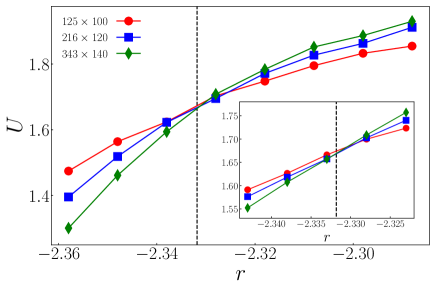
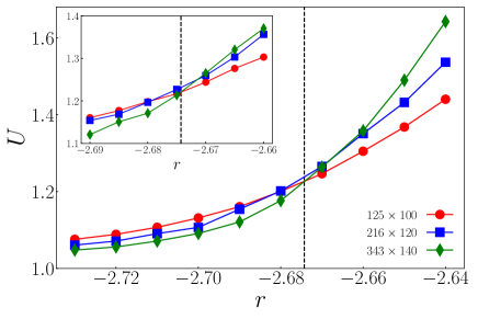
Figure S2: (Color online) Same as Fig. 1, but with $\dot{\gamma}=0.5$ (left) and $\dot{\gamma}=0.01$ (right). The error bars are in the order of the point size.

The critical exponents are estimated by simultaneously fitting the magnetization $\langle\hat{m}\rangle$ and the Binder parameter $U$ to Eqs. (11) and (12). The result is summarized in Tab. S1. Furthermore, we test another estimation method as a consistency check; See the next subsection for details. We list the result in Tab. S1.

	Fitting			At criticality
$\dot{\gamma}$	$\tilde{z}_{h}$	$z_{\tau}$	$\beta$	$\tilde{z}_{h}$	$z_{\tau}$	$\beta$
$5.0$	$-0.980\pm 0.026$	$2.05\pm 0.11$	$0.480\pm 0.029$	$-0.990\pm 0.007$	$1.98\pm 0.01$	$0.500\pm 0.004$
$0.5$	$-0.989\pm 0.028$	$1.83\pm 0.13$	$0.540\pm 0.041$	$-0.941\pm 0.004$	$1.85\pm 0.13$	$0.509\pm 0.036$
$0.01$	$-0.579\pm 0.020$	$2.03\pm 0.20$	$0.285\pm 0.030$	$-0.566\pm 0.004$	$2.14\pm 0.12$	$0.264\pm 0.015$

Table S1: Scaling exponents estimated from the numerical simulation. “Fitting” means the value obtained by fitting the simulation data of $\langle\hat{m}\rangle_{h=0}$ and $U$ to Eqs. (11) and (12). “At criticality” means the one obtained from the data of magnetization at the critical point by using the method explained in Sec. S4.2.

These two estimations are consistent with each other, revealing the validity of our estimation method. We find that the critical exponent $\beta$ for $\dot{\gamma}=5.0$ and $0.5$ is accurately characterized by the mean-field theory. However, for $\dot{\gamma}=0.01$, there is relatively large deviation between the estimation result and the mean-field theory. To make it more clear, we plot the scaled magnetization data in Fig. S3. $\tilde{z}_{h}$ and $z_{\tau}$ are fixed at the mean-field value, $\tilde{z}_{h}=-1$ and $z_{\tau}=2$. For $\dot{\gamma}=0.5$, we find that the scaled data for the different system size are superimposed on a single curve. It means that the finite-size scaling relation Eq. (11) holds with $\tilde{z}_{h}=-1$ and $z_{\tau}=2$. In contrast, for $\dot{\gamma}=0.01$ the scaled data do not overlap as expected. Therefore, the mean-field theory may not be applicable to the case with small shear rate.

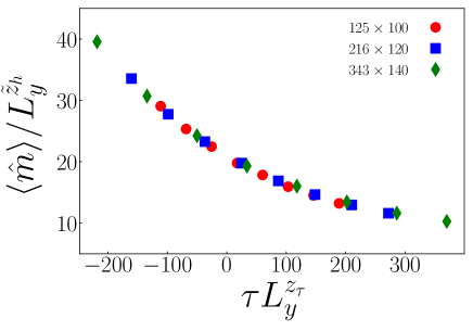
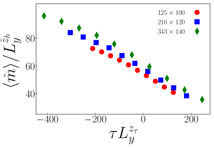
Figure S3: (Color online) The finite-size scaling plot of magnetization. Left: $\dot{\gamma}=0.5$, Right $\dot{\gamma}=0.01$. $\tilde{z}_{h}$ and $z_{\tau}$ are fixed at the mean-field value, $\tilde{z}_{h}=-1$ and $z_{\tau}=2$. The error bars are in the order of the point size.

S4.2 Data at the critical point

As a consistency check, we conduct another estimation method that uses the data at the critical point. Here, we explain the method and the result.

According to the finite-size scaling relation Eq. (11), the magnetization behaves as

$$\langle\hat{m}\rangle_{h=0}=L_{y}^{\tilde{z}_{h}}\mathcal{M}_{1}(\tau=0,L_{y}^{z_{x}}L_{x}^{-1};\dot{\gamma}),$$ (S77)

$$\frac{d\langle\hat{m}\rangle_{h=0}}{d\tau}=L_{y}^{\tilde{z}_{h}+z_{\tau}}\mathcal{M}^{\prime}_{1}(\tau=0,L_{y}^{z_{x}}L_{x}^{-1};\dot{\gamma})$$ (S78)

right at the critical point. Therefore, when the system size increases with $L_{y}^{z_{x}}L_{x}^{-1}$ fixed, the simulation data for $\langle\hat{m}\rangle_{h=0}$ and $d\langle\hat{m}\rangle_{h=0}/d\tau$ are fitted by the simple relations

$$\langle\hat{m}\rangle_{h=0}=aL_{y}^{\tilde{z}_{h}},$$ (S79)

$$\frac{d\langle\hat{m}\rangle_{h=0}}{d\tau}=bL_{y}^{\tilde{z}_{h}+z_{\tau}}.$$ (S80)

Furthermore, from the similar argument, we have the relation for the Binder parameter at the critical point:

$$\frac{dU}{d\tau}=cL_{y}^{z_{\tau}}.$$ (S81)

In Fig. S4, we plot them for $\dot{\gamma}=5.0$, $0.5$, and $0.01$ with a log-log plot. From these figures, we find that all the data can be well described by (S79), (S80), and (S81) as expected from the finite-size scaling theory.

Once we confirm the ansatz of the finite scaling theory, the exponent $\tilde{z}_{h}$ is estimated from the slope of $\langle\hat{m}\rangle_{h=0}$, and the exponent $z_{\tau}$ is estimated from the slope of $d\langle\hat{m}\rangle_{h=0}/d\tau$ or that of $dU/d\tau$. The two estimations of $z_{\tau}$ are in good agreement with each other. We especially choose the exponents obtained from the magnetization and summarize them in Tab. S1. As explained above, the exponents obtained from the data at criticality are consistent with that obtained by fitting the data over a wide region to Eqs. (11) and (12). This result increases the validity of our analysis.

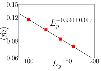
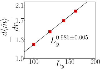
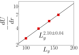
(a) $r=-1.9260$ ($r_{c}=-1.9257$), $\dot{\gamma}=5.0$

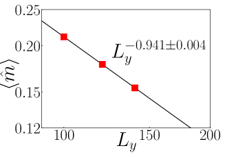
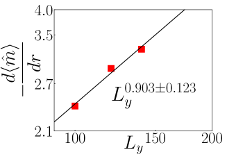
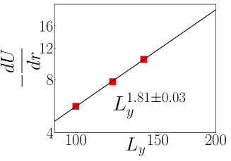
(b) $r=-2.3325$ ($r_{c}=-2.3318$), $\dot{\gamma}=0.5$

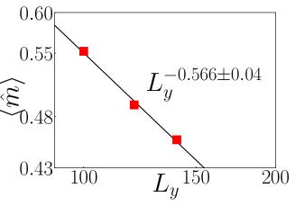
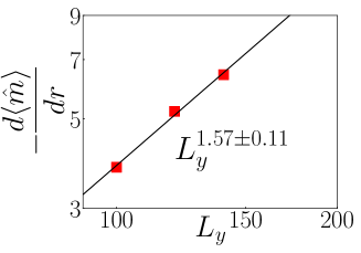
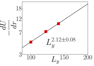
(c) $r=-2.6750$ ($r_{c}=-2.6743$) $\dot{\gamma}=0.01$

Figure S4: (Color online) a log-log plot of the simulation data at the critical point. Left: $\langle\hat{m}\rangle$ versus $L_{y}$. Center: $d\langle\hat{m}\rangle_{h=0}/dr$ versus $L_{y}$. Right: $dU/dr$ versus $L_{y}$.

S4.3 Structure factor slightly above critical point

We numerically calculate the structure factor slightly above the critical point and test whether the value of $z_{x}$ is equal to $3$. In Fig. S5, we show the structure factor $S(\bm{k})$ for $\dot{\gamma}=5.0$ and $r=-1.9255$ ($r_{c}=-1.9257\pm 0.0002$). By using the fact that the structure factor $S(\bm{k})$ behaves as

$$S(\bm{k})=\frac{1}{C_{\tau}\tau^{\omega_{\tau}}+C_{x}k_{x}^{\omega_{x}}+C_{y}k_{y}^{\omega_{y}}}$$ (S82)

slightly above the critical point, we fit the simulation data in $0.0<k_{x}\ {\rm or}\ k_{y}<0.33$ and obtain $\omega_{x}=0.663\pm 0.005$ and $\omega_{y}=1.98\pm 0.01$. Since $\nu_{x}$ and $\nu_{y}$ are written as $\nu_{i}=\omega_{\tau}/\omega_{i}$, $z_{x}$ is calculated as $z_{x}=\nu_{x}/\nu_{y}=\omega_{y}/\omega_{x}=2.99\pm 0.03$. The value $z_{x}=2.99$ is extremely close to $z_{x}=3$. Thus, we again confirm the validity of $z_{x}=3$. We also note that $\omega_{x}=0.663$ and $\omega_{y}=1.98$ are extremely close to that of linearized model, $\omega_{x}=2/3$ and $\omega_{y}=2$ (See Sec. S1.2).

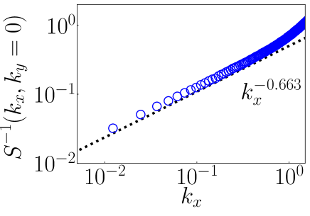
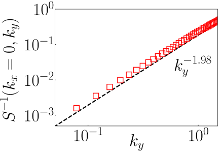
Figure S5: (Color online) Structure factor for $\dot{\gamma}=5.0$. $r$ is chosen as $r=-1.9255$, which is slightly above the critical point ($r_{c}=-1.9257\pm 0.0002$). Left: $S^{-1}(k_{x},k_{y}=0)$ versus $k_{x}$. Right: $S^{-1}(k_{x}=0,k_{y})$ versus $k_{y}$.

The similar calculation is performed for $\dot{\gamma}=0.5$ and $0.01$. Here, we note that the $k_{x}$-dependence of $S^{-1}(k_{x},k_{y}=0)$ crosses over from $k_{x}^{-2/3}$ to $k_{x}^{-2}$ at the length scale $l=\sqrt{\kappa\Gamma/\dot{\gamma}}$. This property is the same as the phase fluctuations explained in the main text. Because the length scale $l$ becomes larger as $\dot{\gamma}$ smaller, it is difficult to estimate the correct value of $\omega_{x}$ from the fitting of $S^{-1}(k_{x},k_{y}=0)$. Then, instead of estimating $\omega_{x}$ and $\omega_{y}$ from the fitting, we compare the simulation data and the straight line with the theoretical values $\omega_{x}=2/3$ and $\omega_{y}=2$. The result is shown in Fig. S6 and the good agreement is found between them, revealing that the structure factor is kept in the linearized form even for small $\dot{\gamma}$.

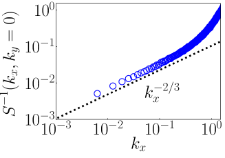
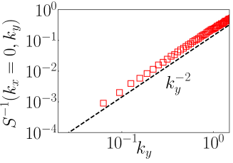
(a) $\dot{\gamma}=0.5$, $r=-2.3280$ ($r_{c}=-2.3318$)

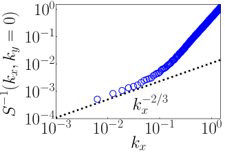
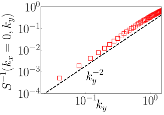
(b) $\dot{\gamma}=0.01$, $r=-2.6700$ ($r_{c}=-2.6743$)

Figure S6: (Color online) Same as Fig. S5, but with (a) $\dot{\gamma}=0.5$ and (b) $\dot{\gamma}=0.01$.

S4.4 Comparison with the previous studies

To summarize our numerical result, (i) the value of the critical exponent $\beta$ is extremely close to the mean-field value for the large shear rate, (ii) it deviates from the mean-field theory when the shear rate becomes small, and (iii) $k_{x}^{-2/3}$ mode (i.e. $\omega_{x}=2/3$) is observed for all the shear rates we have examined.

Here, we compare our result with the ones previously obtained for the sheared Ising model. The pioneer theoretical analysis was carried out for the three-dimensional model H (in the classification of Hohenberg and Halperin) by Onuki and Kawasaki Onuki and Kawasaki (1979). They applied the renormalization group method to the sheared system and showed that the critical exponent $\beta$ is given by the mean-field theory at sufficiently large shear rates. Apart from three-dimensional system, Hucht Hucht (2009) proposed the model that can be solved exactly in the limit of large shear rate and demonstrated that in this limit, $\beta$ is equal to the mean-field value even in the two-dimensional system. Some groups attempted to numerically verify this theoretical prediction Chan and Lin (1990); Winter et al. (2010); Saracco and Gonnella (2009). However, to our knowledge, there was no computational study that observes the mean-field behavior of $\beta$. For example, Chan and Lin reported $\beta=0.38\pm 0.05$ Chan and Lin (1990), Winter et al. $\beta\approx 0.37$ Winter et al. (2010), and Saracco and Gonnella $\beta=0.39\pm 0.01$ (for the largest shear rate) Saracco and Gonnella (2009). Therefore, our study is the first to observe $\beta$ extremely close to the mean-field value for finite shear rate.

The behavior of $\beta$ for small shear rate is still a controversial problem. Our result indicates that it deviates from the mean-field value. However, we do not judge whether this deviation comes from the finite-size effects or remains in the large system-size limit.

S5 Kosterlitz–Thouless transition point in equilibrium

We use the non-equilibrium relaxation method for determining the Kosterlitz–Thouless transition point $r_{KT}$ in equilibrium. It is the method that estimates the position of the critical point from the dynamical properties around the critical point. We below summarize the concrete procedure. See Ref. Ozeki et al. (2003); Ozeki and Ito (2007) for details of non-equilibrium relaxation method.

Let us consider the relaxation process of the magnetization $\langle\hat{m}_{a}\rangle(t)$ from the all-aligned state $\varphi_{1}(\bm{r})=1$ and $\varphi_{2}(\bm{r})=0$, where $\hat{m}_{a}$ is defined by

$$\hat{m}_{a}=\frac{1}{L_{x}L_{y}}\int d^{2}\bm{r}\varphi_{a}(\bm{r}).$$ (S83)

For the disordered state (i.e. $r>r_{KT}$), the magnetization $\langle\hat{m}_{a}\rangle(t)$ exhibits the exponential decay:

$$\langle\hat{m}_{x}\rangle(t)\sim\exp\Big{(}-\frac{t}{\tau_{rel}(r)}\Big{)},$$ (S84)

where $\tau_{rel}(r)$ is the relaxation time. The theoretical calculation predicts that the relaxation time $\tau_{rel}(r)$ diverges as $r\to r_{KT}+0$ in the form

$$\tau_{rel}(r)=B\exp\Big{(}\frac{A}{\sqrt{r-r_{KT}}}\Big{)}.$$ (S85)

Based on this property, we can estimate $r_{KT}$ from observing the divergence of relaxation time.

In order to calculate the relaxation time $\tau_{rel}(r)$ in the numerical simulation, we use the dynamical scaling relation that holds near the critical point:

$$\langle\hat{m}_{x}\rangle(t)=\tau_{rel}(r)^{\lambda}\tilde{m}\Big{(}\frac{t}{\tau_{rel}(r)}\Big{)},$$ (S86)

where $\lambda$ is the dynamical exponent. Because $\lambda$ is a universal constant, we assume that $\lambda$ is given by the value, 0.068, obtained in the previous study Ozeki et al. (2003). We present the numerical calculation result of $\langle\hat{m}_{x}\rangle(t)$ and its scaling plot in Fig. S7. The system size is chosen as $L_{x}=L_{y}=512$, and we take an ensemble average over $120$ noise realizations. While $\tau_{rel}(r)$ hardly depends on the system size far from the transition point $r_{KT}$, a larger system size is required to exactly measure $\tau_{rel}(r)$ very near the transition point $r_{KT}$. To depict the scaling plot, we choose the magnetization curve with $r=-2.75$ as the reference curve, specifically, $\tau_{rel}(r=-2.75)$ is fixed at $1.0$, and fit the magnetization curves with $r=-2.895,-2.89,-2.885,-2.88,-2.875,-2.87,-2.86,-2.85,-2.84,-2.83,-2.82,-2.81$ to the reference curve. The best-fit parameter $\tau_{rel}$ is depicted in Fig. S8 as a function of $r$. It is well fitted by Eq. (S85) with $A=5.6190\pm 0.4300$, $\log B=-10.820\pm 0.6868$ and $r_{KT}=-3.0204\pm 0.0087$. Accordingly, the Kosterlitz–Thouless transition point is estimated as $r_{KT}=-3.0204\pm 0.0087$.

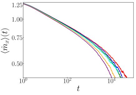
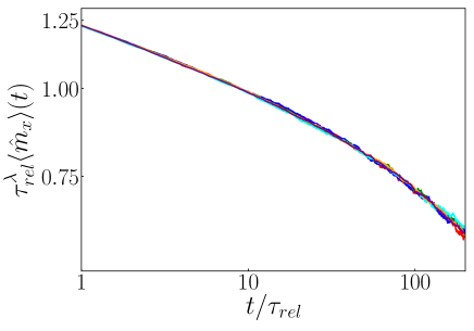
Figure S7: (Color online) Left: relaxation of magnetization from the all-aligned state for $r=-2.895,-2.89,-2.885,-2.88,-2.87,-2.86$ with a log-log plot. Right: $\tau_{rel}^{\lambda}\langle\hat{m}_{x}\rangle(t)$ versus $t/\tau_{rel}$ calculated from the left figure. Each curve is shifted by $\lambda=0.068$ and $\tau_{rel}=158.0,110.0,84.0,69.0,37.0,25.0$.

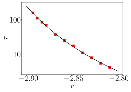
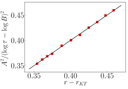
Figure S8: (Color online) Relaxation time $\tau_{rel}$ as a function of $r$. Left: $\tau_{rel}$ versus $r$. Right: $A^{2}/(\log\tau_{rel}-\log B)^{2}$ versus $r-r_{KT}$. The black solid curve represents Eq. (S85) with $A=5.6190$, $\log B=-10.820$ and $r_{KT}=-3.0204$.

Furthermore, we measure the helicity modulus $\Upsilon$ in equilibrium state Weber and Minnhagen (1988), which is defined as follows Fisher et al. (1973); Ohta and Jasnow (1979). Let us consider the twisted periodic boundary condition along $x$ direction

$$\bm{\varphi}(x+L,y,t)=R(\Delta)\bm{\varphi}(x,y,t),$$ (S87)

where $R(\Delta)$ is the rotation matrix

$$R(\Delta)=\begin{pmatrix}\cos\Delta&-\sin\Delta\\ \sin\Delta&\cos\Delta\end{pmatrix}.$$ (S88)

The free energy depends on the twisted angle $\Delta$. We write it as $F(T,\Delta,L)$, where $T$ is the temperature and $L$ is the system size $L_{x}=L_{y}$. The free energy $F(T,\Delta,L)$ is expanded in the form

$$F(T,\Delta,L)=F(T,0,L)+\frac{\partial F(T,\Delta,L)}{\partial\Delta}\Big{|}_{\Delta=0}\Delta+\frac{1}{2}\frac{\partial^{2}F(T,\Delta,L)}{\partial\Delta^{2}}\Big{|}_{\Delta=0}\Delta^{2}+\cdots,$$ (S89)

where $F(T,0,L)$ is the free energy under the standard periodic boundary condition. Because the system is invariant under $\Delta\to-\Delta$, we have

$$\frac{\partial F(T,\Delta,L)}{\partial\Delta}\Big{|}_{\Delta=0}=0.$$ (S90)

Furthermore, $F(T,\Delta,L)\geq F(T,0,L)$ holds because the global minimum of free energy corresponds to the non-twisted state. We thus obtain

$$\frac{\partial^{2}F(T,\Delta,L)}{\partial\Delta^{2}}\Big{|}_{\Delta=0}\geq 0.$$ (S91)

Based on these properties, the helicity modulus $\Upsilon$ is defined as

$$\Upsilon(L)=\frac{\partial^{2}F(T,\Delta,L)}{\partial\Delta^{2}}\Big{|}_{\Delta=0}.$$ (S92)

We here introduce $\Upsilon_{\infty}\equiv\lim_{L\to\infty}\Upsilon(L)$. Intensive studies revealed that $\Upsilon_{\infty}$ jumps at the Kosterlitz–Thouless transition point $r_{KT}$ from zero (in disordered state) to $2T/\pi$ (in quasi-long-range ordered state) Weber and Minnhagen (1988); Schultka and Manousakis (1994); Olsson (1995), and that the finite-size corrections are given by

$$\Upsilon(L)=\frac{2T}{\pi}\Big{(}1+\frac{1}{2}\frac{1}{\log L+{\rm const}}\Big{)},$$ (S93)

which was derived by Weber and Minnhagen Weber and Minnhagen (1988). Note that higher-order corrections were discussed in Ref. Hasenbusch (2005).

We test Eq. (S93) near $r=-3.0204$ and confirm the validity of the transition point obtained by the non-equilibrium relaxation method. Fig. S9 presents the helicity modulus calculated in the numerical simulations. The system size is chosen as $L=32,64,128,256$. We take an average over $10^{6}$ different times at $t=100i\delta t$ for $8$ noise realizations. We will later explain the microscopic expression used to calculate the helicity modulus.

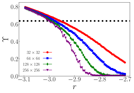
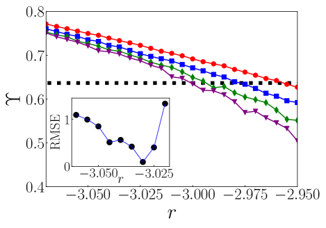
Figure S9: (Color online) Plot of helicity modulus for four different system sizes. Left: $\Upsilon$ versus $r$. Right: zoom around $r=-3.00$. Inset: root mean square error (RMSE) of fit to Eq. (S94) at each $r$. The minimum point gives the Kosterlitz–Thouless transition point.

In the left side of Fig. S9, we observe the onset of the helicity modulus from zero to the finite value. As shown in Eq. (S93), the helicity modulus at $r=r_{KT}$ approaches $2T/\pi$ in the limit $L\to\infty$, which is depicted by the black dotted line. Because the helicity modulus for $L=256$ takes a value close to $2T/\pi$ at $r=3.0$, we plot the zoom of this region in the right side of Fig. S9.

Then, we fit the simulation data at each $r$ to Eq. (S93) by using the least squares method. For this purpose, we rewrite Eq. (S93) into

$$\Big{(}\Upsilon(L)\frac{\pi}{2T}-1\Big{)}^{-1}=2\big{(}\log L+{\rm const}\big{)},$$ (S94)

and const is treated as a free parameter. The root mean square error (RMSE) of fit to Eq. (S94) is presented in the inset of the right side of Fig. S9. It takes a minimum at $r=-3.03$, which means that the Kosterlitz–Thouless transition point $r_{KT}$ is located near $r=-3.03$. We show the simulation data (red square) and the best-fit curve (black solid) at $r=-3.03$ in Fig. S10. To make it easier to see, it is organized in the form of Eq. (S94). From this figure, we confirm the validity of our fitting result.

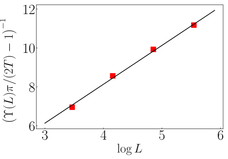
Figure S10: (Color online) $\Upsilon$ versus $L$ at $r=-3.03$.

The calculation result using the helicity modulus is in reasonable agreement with that by the non-equilibrium measurement method. This consistency justifies the non-equilibrium measurement method and we conclude that $r_{KT}=-3.0204\pm 0.0087$.

Microscopic expression of helicity modulus

To calculate the helicity modulus in numerical simulations, we derive a microscopic expression of helicity modulus. We start with the spatially-discretized Landau free energy:

$$\Phi[\bm{\varphi}]=(\delta x)(\delta y)\sum_{i_{x},i_{y}}\Big{\{}\frac{\kappa}{2}\sum_{a=1}^{2}\Big{(}\frac{\varphi_{a}^{i_{x}+1,i_{y}}-\varphi_{a}^{i_{x},i_{y}}}{\delta x}\Big{)}^{2}+\frac{\kappa}{2}\sum_{a=1}^{2}\Big{(}\frac{\varphi_{a}^{i_{x},i_{y}+1}-\varphi_{a}^{i_{x},i_{y}}}{\delta y}\Big{)}^{2}+\frac{r}{2}|\bm{\varphi}^{i_{x},i_{y}}|^{2}+\frac{u}{4}\big{(}|\bm{\varphi}^{i_{x},i_{y}}|^{2}\big{)}^{2}\Big{\}},$$ (S95)

where $\delta x$ and $\delta y$ are the space interval. This Landau free energy yields Eq. (3) in the continuum limit.

Instead of considering the system under the twisted periodic boundary condition Eq. (S87), we introduce the twisted Landau free energy

$$\Phi[\bm{\varphi};\Delta]=(\delta x)(\delta y)\sum_{i_{x},i_{y}} \Big{\{}\frac{\kappa}{2}\sum_{a=1}^{2}\Big{(}\frac{\psi_{a}^{i_{x}+1,i_{y}}(\Delta)-\psi_{a}^{i_{x},i_{y}}(\Delta)}{\delta x}\Big{)}^{2}+\frac{\kappa}{2}\sum_{a=1}^{2}\Big{(}\frac{\psi_{a}^{i_{x},i_{y}+1}(\Delta)-\psi_{a}^{i_{x},i_{y}}(\Delta)}{\delta y}\Big{)}^{2}$$ (S96)

$$+ \frac{r}{2}|\bm{\psi}^{i_{x},i_{y}}(\Delta)|^{2}+\frac{u}{4}\big{(}|\bm{\psi}^{i_{x},i_{y}}(\Delta)|^{2}\big{)}^{2}\Big{\}}$$

with

$$\bm{\psi}^{i_{x},i_{y}}(\Delta)=R\Big{(}\frac{\Delta}{L}i_{x}\delta x\Big{)}\bm{\varphi}^{i_{x},i_{y}},$$ (S97)

and study this system under the standard periodic boundary condition. These two systems are equivalent to each other with respect to thermodynamic properties.

The free energy is given by

$$F(T,\Delta,L)=-\frac{1}{T}\log\int\Big{(}\prod_{i_{x},i_{y}}d^{2}\bm{\varphi}^{i_{x},i_{y}}\Big{)}e^{-\Phi[\bm{\varphi};\Delta]/T}.$$ (S98)

By substituting Eq. (S98) into the definition of the helicity modulus $\Upsilon$, Eq. (S92), we obtain the microscopic expression of the helicity modulus:

$$\Upsilon = -\frac{\kappa}{T}\Big{(}\frac{\delta x}{L}\Big{)}^{2}(\delta y)^{2}\Big{\{}\Big{\langle}\Big{(}\sum_{i_{x},i_{y}}\Big{[}\varphi_{1}^{i_{x},i_{y}}\varphi_{2}^{i_{x}+1,i_{y}}-\varphi_{2}^{i_{x},i_{y}}\varphi_{1}^{i_{x}+1,i_{y}}\Big{]}\Big{)}^{2}\Big{\rangle}-\Big{\langle}\sum_{i_{x},i_{y}}\Big{[}\varphi_{1}^{i_{x},i_{y}}\varphi_{2}^{i_{x}+1,i_{y}}-\varphi_{2}^{i_{x},i_{y}}\varphi_{1}^{i_{x}+1,i_{y}}\Big{]}\Big{\rangle}^{2}\Big{\}}$$ (S99)

$$+ \Big{(}\frac{\delta x}{L}\Big{)}^{2}(\delta y)\Big{\langle}\sum_{i_{x},i_{y}}\Big{[}\varphi_{1}^{i_{x},i_{y}}\varphi_{1}^{i_{x}+1,i_{y}}+\varphi_{2}^{i_{x},i_{y}}\varphi_{2}^{i_{x}+1,i_{y}}\Big{]}\Big{\rangle}.$$

The numerical results in the previous subsection were obtained by using this expression.