Automated Model Compression by Jointly Applied Pruning and Quantization

Abstract

Although deep neural networks (DNNs) achieve excellent performance in real-world computer vision tasks, network compression may be necessary to adapt DNNs into edge devices such as mobile phones. In the traditional deep compression framework, iteratively performing network pruning and quantization can reduce the model size and computation cost to meet the deployment requirements. However, such a step-wise application of pruning and quantization may lead to suboptimal solutions and unnecessary time consumption. In this paper, we tackle this issue by integrating network pruning and quantization as a unified joint compression problem, and then use AutoML to automatically solve it. We find the pruning process can be regarded as the channel-wise quantization with 0 bit. Thus, the separate two-step pruning and quantization can be simplified as the one-step quantization with mixed precision. This unification not only simplifies the compression pipeline but also avoids the compression divergence. To implement this idea, we propose the Automated model compression by Jointly applied Pruning and Quantization (AJPQ). AJPQ is designed with a hierarchical architecture: the layer controller controls the layer sparsity and the channel controller decides the bitwidth for each kernel. Following the same importance criterion, the layer controller and the channel controller collaboratively decide the compression strategy. With the help of reinforcement learning, our one-step compression is automatically achieved. Compared with the state-of-the-art automated compression methods, our method obtains a better accuracy while reducing the storage considerably. For fixed precision quantization, AJPQ can reduce more than $5\times$ model size and $2\times$ computation with a slight performance increase for Skynet in the remote sensing object detection. When mixed precision is allowed, AJPQ can reduce $5\times$ model size with only ${1.06\%}$ top-5 accuracy decline for MobileNet in the classification task.

Introduction

Although deep neural networks (DNNs) achieve excellent performance in real-world computer vision tasks, network compression may be necessary to adapt DNNs into edge devices such as mobile phones and surveillance camera (Zou et al. 2019). To obtain a balance between the model’s performance and reduction, different approaches of model compression are proposed such as knowledge distillation, network pruning and binary convolutional network (Hinton, Vinyals, and Dean 2015; Han et al. 2015; Rastegari et al. 2016), etc.

Either network pruning or network quantization can achieve model compression by reducing the size or bitwidth of weights. However, those compression techniques sometimes can be heavy-duty of human work requiring a tedious parameter adjusting process. Although some criterions (Li et al. 2017; Han et al. 2015) can help to identify redundant connections during pruning, it may involve manual work to decide proper layer sparsity. Likewise, when mixed precision (Elthakeb et al. 2018) is introduced to fully leverage advantages of the cutting-edge hardware, the appropriate combination of each layer’s or kernel’s bitwidth needs to be manually explored. To address this issue, the AutoML technique is introduced to perform automated compression (He et al. 2018; Manessi et al. 2018; Wang et al. 2019; Gao et al. 2019). In these methods, the deep compression framework proposed by Han, Mao, and Dally (2016) contains a three stage pipeline: pruning, quantization and Huffman coding to reduce the storage step by step. To further improve the performance for each step, they utilize the AutoML(Automated Machine Learning) to perform automated pruning (He et al. 2018) and automated quantization (Wang et al. 2019), respectively.

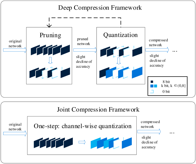
Figure 1: The deep compression (Han, Mao, and Dally 2016) and our joint compression. The deep compression framework applies network pruning and quantization step by step, which means network quantization only starts when pruning finish. Based on compression requirements, our joint compression framework can spontaneously switch among different compression techniques for different layers.

Figure 1 illustrates the framework of the deep compression. In the pruning phase, deep compression takes the original network as input, and then removes the unnecessary connections, outputting a pruned model. In the quantization phase, deep compression takes the pruned network as input, and then produces a nearly lossless compressed model represented by the integer weights. In each phase, the optimal compression can be achieved because the AutoML technique can search the most available compression strategy according to hardware constraint. However, in the view of the whole compression, this simple combination of pruning and quantization is suboptimal. The pruning and quantization should interact with each other to achieve the global optimal balance between the performance holding and computation reduction, rather than their own optimum. What’s more, because two optimization problems need solving, this step-wise design is time consuming.

To tackle this issue, we incorporate the pruning and quantization into a joint compression framework, and then use AutoML to jointly search the globally optimal compression strategy. Specifically, we find the pruning process can be regarded as the channel-wise quantization with 0 bit. Thus, the separate two-step pruning and quantization can be simplified as the one-step quantization with mixed precision. Thanks to this simplification, our framework has the potential to provide a better compression solution than the deep compression framework. A challenge for our framework is how to perform the channel-wise quantization with mixed precision from 0 to $N$ bits. Because each channel has many candidate bits, the searching space is large. For this reason, the current automated quantization methods usually perform mixed precision across different layers (Wang et al. 2019; Elthakeb et al. 2018) (layer number is much less than channel number). In this paper, we design a novel hierarchical architecture: the layer controller controls the layer sparsity and the channel controller decides the bitwidth for each channel. Following the same importance criterion, the layer controller and channel controller collaboratively decide a quantization plan for the whole network. In this way, we solve the inefficiency problem.

Technically speaking, we propose Automated Model Compression by Jointly applied Pruning and Quantization (AJPQ) as shown in Figure 2. Inspired by layer sparsity control in AMC (He et al. 2018), AJPQ’s layer controller can automatically search the optimal preserved ratio in continuous space for each layer by DDPG(Deep Deterministic Policy Gradient) (Silver et al. 2014). With reduction achieved by removing trivial channels, the channel controller only needs to decide the non zero bitwidth for the rest of the channels, whose number is reduced. By using size constraint as the upper bound and applying weight importance to compute the lower bound, greedy searching is capable of quickly generating a quantization plan for each layer. For this plan, the environment (hardware) will respond with the state information and reward to the agent to help correct the quantization plan in the next iteration.

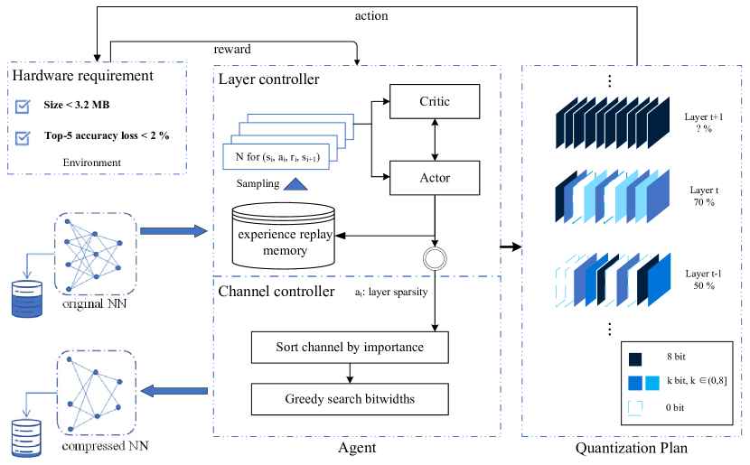
Figure 2: Overview of the Automated Model Compression by Jointly applied Pruning and Quantization (AJPQ) engine. For specific compression requirements and a model, AJPQ searches the quantization plan layer by layer. At each layer, the layer controller decides the layer sparsity, and then the kernel controller determines the bit -width for preserved channels. After searching the quantization plan for specific episodes, AJPQ outputs a compressed model by the quantization plan with the highest reward.

In summary, our contributions can be concluded in the three aspects:

• A joint compression framework is proposed to accelerate the searching for a globally optimal compression strategy while retaining the performance of the compressed model.

• We propose a new viewpoint that pruning process can be regarded as the channel-wise quantization with 0 bit, and furthermore, gives a hierarchical architecture to efficiently and automatically solve the channel-wise quantization with mixed precision.

• We evaluate AJPQ approach with the state-of-the-art automated compression tools AMC (He et al. 2018) and HAQ (Wang et al. 2019) on MobileNet (Howard et al. 2017) and Skynet. A better performance with less time consumption is achieved. What’s more, AJPQ can reduce more than $5\times$ model size and $2\times$ computation while achieving the performance with $4.5\%$ improvement for Skynet in the remote sensing object detection.

The following sections are orginzed as follow: previous work in network compression is summarized in Related Work; detailed design of AJPQ is presented in Methodology; effectiveness of AJPQ for the classification and detection is presented in Experimental Results; conclusion and further improvement is in Conclusion.

Related Work

As network pruning can be defined as a channel selection problem followed by a specific criterion, extensive works focus on evaluating the redundancy or importance of channels. For example, the weight values of connections are initially used to evaluate the importance of connections in a trained model (Li et al. 2017; Han et al. 2015; He et al. 2019; Zhuang et al. 2018; Ye et al. 2018). In contrast to directly utilizing trained weights, He et al. (2019) represent the common information by geometric median among filters as an attempt to overcome the ”small norm deviation” and ”large minimum norm” problems brought by the norm-based criterion (Li et al. 2017). Anwar, Hwang, and Sung (2017) identify the trivial and redundant connection by a genetic algorithm to adapt to the different pruning particle. Although these criteria are efficient in computation and application, defining preserve ratio or sparsity for each layer is manual work.

To get rid of the tedious process of parameter adjustment, (Zhuang et al. 2018; Ye et al. 2018; Liu et al. 2019; Luo, Wu, and Lin 2017; Zhu and Gupta 2018; Gao et al. 2019) train a pruned network from the scratch. For example, Zhuang et al. (2018) augment the meaning of channel importance with the discriminative power. Ye et al. (2018) form the channel selection as an optimization problem and solve it by ISTA(Iterative Shrinkage-Thresholding Algorithm) in batch normalization applied DNNs. Inspired by NAS (Zoph and Le 2017), (Liu et al. 2019) keeps the model with the best performance from a set of random generated pruned models.

As the pruning process can be defined as a Markov decision process (Bertsekas 1995), techniques in AutoML(Automated Machine Learning) domain are applied to efficiently search the compression plan in a layer-by-layer manner (Elthakeb et al. 2018; He et al. 2018; Wang et al. 2019; Ashok et al. 2018). To support deep quantization which allows mixed precision in network representation, HAQ and ReLeQ (Wang et al. 2019; Elthakeb et al. 2018) are proposed while ReLeQ (Elthakeb et al. 2018) requires a fine-tuning stage beside the reinforcement learning searching loop. Those reinforcement learning approaches enable more controls during pruning or quantization related schedule process.

After deep compression framework (Han, Mao, and Dally 2016), plenty of works are inspired (Manessi et al. 2018; He et al. 2018; Chen, Emer, and Sze 2017; Wen et al. 2016; Zhu and Gupta 2018). For example, (Manessi et al. 2018), (He et al. 2018) and (Zhu and Gupta 2018) aim to automatically prune connections. While Manessi et al. (2018) improve the threshold-based channel selection in (Han, Mao, and Dally 2016). (Zhu and Gupta 2018) and (He et al. 2018) schedule preserve ratio for each layer by a sparsity function and RL agent respectively. To achieve a considerable reduction in convolutional layers of the pruning process in deep compression, (Wen et al. 2016) proposes to learn the structured sparsity. Utilizing the deep compression framework, (Chen, Emer, and Sze 2017) deploys an energy-efficient model for real-world application.

There are also explorations to achieve one-step compression without following the deep compression framework such as NAS(Neural architecture search) (Zoph and Le 2017) and binary convolutional network (Rastegari et al. 2016). Considering the high computations resource requirements, NAS may not be an economical solution for general usage. The binary convolutional network may be the answer, but it cannot replace all existing useful DNNs so far.

Overall, AJPQ automatically achieves the pruning and quantization in the one-step compression, which is different from the above works.

Figure 3: Roles for layer and channel controller in our method. Guided by the same importance criterion at each layer, the agent generates a quantization plan to deliver positive reward with respect to the performance and compression. The quantization plan is generated by the layer controller and the channel controller together: the layer controller decides channels with zero bit-width; the controller decides non-zero bit-width for the preserved channels.

Methodology

Following the joint compression framework, the AJPQ is proposed for searching the quantization plan. The layer-wise searching for a proper quantization plan can be formulated as a dynamic programming problem. Considering a DNN model with $n$ quantizable layers and the channel number for each layer is represented by $I^{l},l=1,...,n$, thus $\mathcal{I}=\{I_{1},...,I_{n}\}$, our goal is to balance the performance and storage by assigning each channel with the proper bitwith. Let us denote that $s_{l}$ is an environment state, $P^{l}$ is a channel-wise quantization plan, $r_{l}$ is the reward of the generated channel-wise quantization plan.We assume that $r_{0},r_{1},...,r_{n-1}$ are independent. Thus, the quantization state changes as follows:

$$s_{l+1}=f(s_{l},P^{l},r_{l})$$ (1)

For the $l$-th layer, the problem space is $(bit_{max}+1)^{I_{l}}$ with allowed the bitwidth in [0, $bit_{max}$], where the $bit_{max}$ is the maximal allowed bitwidth and is set as 8 in default. Because $(bit_{max}+1)^{I_{l}}$ is very large, the amount of the possible permutations of $P^{l}$ is massive. The previous work has shown that eliminating the redundant channels in a trained model is nearly lossless (He et al. 2019), thus, removing the trivial channels will make the problem space shrink. A widely used metric to measure the channel’s redundancy is the importance score $\{imp_{i}^{l}|i=1,...,I_{l}\}$, which is computed by the $L1$-norm of the corresponding kernel values in the $l$-th layer (Li et al. 2017). For the preserved channels, we narrow the searching space by the assumption that the more important a channel is, the longer bitwidth it should hold. Therefore, by using the identical importance score $imp_{i}^{l}$, the minimal bitwidth $minbit^{l}_{c}$ is computed for the $c$-th preserved channel. $minbit^{l}_{c}$ is used as the lower bound in the searching, and the upper bound is $bit_{max}$. So the problem space is shrunk to $\prod_{c=1}^{c_{nz}^{l}}(bit_{max}-minbit^{l}_{c}$, where $c_{nz}^{l}$ is the number of nonzero bitwith channels. With the approaching goal and a narrowed searching space, the non-zero mixed bitwidths $\mathcal{B}=\{b_{1},...,b_{c_{nz}^{l}}\}$ for the preserved channels should be solved by a greedy algorithm without dramatic performance decline. In this way, this dynamic programming problem is efficiently optimized.

Specifically, the layer controller in our method identifies the redundancy, and predicts the layer sparsity by DDPG (Silver et al. 2014). The channel controller performs channel selection and decides the different bitwidths for the nontrivial channels by a greedy algorithm.

Algorithm 1 Produce quantization plan for the whole network

Input : $\mathcal{N}$, $\mathcal{N}_{size}$, $n$, $\mathcal{I}$, $\mathcal{N^{\prime}}_{size}$, each layer’s size $S$, total searching episodes $e$, required model compression ratio $sc$, upper bound of the bitwidth $bit_{max}$;

1:  Initialize $s_{0}$ represented by Equation (2) and the current searching episodes $e_{cur}=0$

2:  while $e_{cur}<e$ do

3:     $l=0$, $P=\{bit_{max}\}$

4:     Initialize the critic network $\mu$, the actor network $\theta$, exploration noise $\sigma=0.9$, each quantizable layer size $S=\{S^{l}|l=1,...,n\}$ by original model $\mathcal{N}$

5:     while $l<n$ do

6:        $a_{l}=TN(\mu(s_{l}|\theta_{l}^{\mu}),\sigma^{2},0,1))$

7:        Compute the number of nonzero bit channels $c_{nz}^{l}=min(I^{l},max(1,\lceil I^{l}\times a_{l}\rceil))$

8:        Compute $imp^{l}_{i}=\left|\sum_{i=1}^{i=I^{l+1}}(F^{l}_{i})\right|$ by the value of the according filters $F^{l}_{i}$

9:        Sort $imp_{i}^{l}$ in the descending order

10:        Compute index of the preserved channels $I_{nz}^{l}$ = $top_{c_{nz}^{l}}\{imp_{i}^{l}|,i=1,...,I_{l}\}$

11:        For $i\notin I_{nz}^{l}$, $P^{l}_{i}=0,minbit^{l}_{i}=0$

12:        For $i\in I_{nz}^{l}$, $P^{l}_{i}=bit_{max}$, $minbit^{l}_{i}=bit_{max}\times\frac{imp^{l}_{i}}{\max\limits_{c}(imp^{l}_{c})}$

13:        Update $S^{l}$, $\mathcal{N}_{size}$ by quantization plan $P^{l}$

14:        if $l$ == $n-1$ then

15:           while $\mathcal{N^{\prime}}_{size}>sc\times\mathcal{N}_{size}$ do

16:              $l^{\prime}=\max\limits_{i\in{1,...,n}}(S^{i})$

17:              $c^{\prime}=\min\limits_{j\in I_{nz}^{l}}(imp_{j}^{l})$

18:              if $P^{l^{\prime}}_{c^{\prime}}>minbit^{l^{\prime}}_{c^{\prime}}$ then

19:                 $P^{l^{\prime}}_{c^{\prime}}=P^{l^{\prime}}_{c^{\prime}}-1$

20:              end if

21:              Update $S^{l}$, $\mathcal{N}_{size}$ by quantization plan $P^{l}$

22:           end while

23:        end if

24:        Update reward $r_{l}$ by Equation (3) and $S_{l}$

25:        $l$ = $l$ + 1

26:     end while

27:     Update layer controller with $a_{l}$, $s_{l}$ by DDPG (Silver et al. 2014)

28:     $e_{cur}$ = $e_{cur}$ + 1

29:  end while

Layer Controller

Reinforcement learning is deployed for identifying layer sparsity $a_{l}$, which means the ratio between the number of nonzero bit channels and the total amount of original channels. As we define that $a_{l}\in(0,1]$, the DDPG algorithm is used to solve the continuous action space of $a_{l}$.

State Space: The state space $\mathcal{M}=\{s_{l}|l=1,...,n\}$ is a finite set consisting of all quantizable layers for the model to be compressed. The state $s_{l}$ is characterized by the following features:

$$\begin{split}(idx,t,c_{o}^{l},c_{i}^{l},w,h,stride,k,reducedFLOPs,\\ restFLOPs,reducedSize,restSize,a_{l-1})\end{split}$$ (2)

where for a quantizable layer, $idx$ is the index, $t$ is the type of layer (fully connected layer or convolutional layer). $c_{o}^{l}$ is the number of output channels and $c_{i}^{l}$ is the number of input channels. $w$, $h$ are width and height for each input feature map. $stride$, $k$ are the value of the stride and kernel size which will be 0 and 1 for fully connected layer, respectively. $reducedFLOPs$ and $restFLOPs$ are the numbers of the reduced and the rest FLOPs for the current quantization plan; $reducedSize$ and $restSize$ are the amounts of the reduced and the rest storage for the current quantization plan. The state is normalized at each update because it is friendly for actor and critic network (Ashok et al. 2018). As agent explores in a layer-by-layer manner, such features are required to seek a proper quantization plan.

Reward: The reward is used to evaluate the captured trade-off by comparing the performance and the model size between the compressed model $\mathcal{N^{\prime}}$ and the original model $\mathcal{N}$. For $\mathcal{N}$ on classification task, the top-5 accuracy is $\mathcal{N}_{acc}$; for $\mathcal{N}$ on detection task, the average precision(AP) with IoU(intersection over union)=0.3 is $\mathcal{N}_{AP}$. $\mathcal{N}_{size}$ is the original model size. Our goal is compressing model $\mathcal{N}$ within the $s\times\mathcal{N}_{size}$, where $s$ is decided by the hardware constraints and $s\in(0,1]$. The reward $r$ is derived by:

$$r=\left\{\begin{matrix}-10.0&,\mathcal{N^{\prime}}_{size}>s\times\mathcal{N}_{size}\\ 0.1\times(\mathcal{N}^{\prime}_{acc}-\mathcal{N}_{acc})&,\mathcal{N^{\prime}}_{size}\leq s\times\mathcal{N}_{size}\\ \mathcal{N}^{\prime}_{AP}-\mathcal{N}_{AP}&,\mathcal{N^{\prime}}_{size}\leq s\times\mathcal{N}_{size}\end{matrix}\right.$$ (3)

Methods	Accuracy	Accuracy	Compressed	FLOPs	Searching
	(top-1)	(top-5)	ratio (bit)	ratio	episodes
AMC+Fixed	66.214($\downarrow$5.426)	85.330($\downarrow$4.14)	0.2484	0.8005	500
AJPQ (Fixed)	67.020($\downarrow$4.62)	87.110($\downarrow$2.36)	0.214	0.817	500
AMC+HAQ (layer-wise)	66.690($\downarrow$4.95)	85.2($\downarrow$4.27)	0.207	0.8005	900
AJPQ (layer-wise)	66.280($\downarrow$5.36)	87.00($\downarrow$2.47)	0.195	0.808	500
AJPQ (channel-wise)	69.480($\downarrow$2.16)	88.410($\downarrow$1.06)	0.189	0.922	100

Table 1: The accuracy, compressed ratio, and FLOPs ratio achieved by AMC (He et al. 2018), HAQ (Wang et al. 2019), and our method on MobileNet.

Channel Controller

The channel controller is responsible for deciding the permutation of the bit-widths for the preserved channels. As shown in Algorithm 1, the number of preserved channels $c_{nz}^{l}$ is identified by layer sparsity $a_{l}$ at $l$-th layer. Then based on $c_{nz}^{l}$ and channels’ importance $imp^{l}$, index of preserved channels $I_{nz}^{l}$ is identified. For greedy searching a quantization plan, the lower bound is represented by the minimal bit-width $minbit$, and the upper bound is the maximal allowed bitwidth $bit_{max}$. When the compressed model size is larger than the size constraint, the channel controller first selects a layer and then declines the bit-width from the trivial channels. The channel controller is also compatible with the layer-wise quantization and the fixed precision quantization. Either the layer-wise quantization or the fixed precision is a special case of the channel-wise quantization. What’s more, two layer selection rules are implemented in the AJPQ. The ”large layer first” rule selects the layer with the largest layer size from all quantizable layers, the “deep layer first rule” adjusts the quantization plan from the deepest quantizable layer.

Joint Decision

As stated before, each layer’s quantization plan is a joint decision made by the layer controller and the channel controller. A hierarchical structure is designed to fulfill this target as shown in Figure 3. An identical importance criterion guides the process of eliminating the redundancy and preserving channels. After the layer controller deciding a layer sparsity, the channel controller acts like a regulator: retaining the preserved channels with a high bit-width when the layer sparsity is too high to maintain the performance and reducing some preserved channels’ bitwidth when the layer sparsity is too low to perform necessary compression. In this way, the elements associated with the trimmed channels’ are set to 0 bit, while the other elements are retained in the proper bitwidth. Our method is concluded in Algorithm1.

Experimental Results

Experiment Setting

Data set and Model: For classification, 20,000 images of ImageNet(Deng et al. 2009) is used for state initialization and performance recovery; while 10,000 images of it is used for the validation. For detection, a remote sensing data-set containing bay area, coastline and ocean with 5702 images is used; While 1900 for validation and 3801 for state initialization and performance recovery. In the following experiments, we compare our method with the baselines on MobileNet(Howard et al. 2017) for classification and Skynet(Zhang et al. 2020) for detection. Skynet is a new hardware-efficient DNN specialized in object detection and tracking in aerial images. It only contains 6 depth-wise separable convolution(Howard et al. 2017) blocks for feature extraction.
Metrics: Top-1 and top-5 accuracy are used to estimate the performance of the compressed model in the classification task; AP (Average Precision) is used to evaluate the performance of the compressed model in the detection task. For the compressed model $\mathcal{N^{\prime}}$ with the computation $\mathcal{N^{\prime}}_{c}$ and model size $\mathcal{N^{\prime}}_{s}$, the original model $\mathcal{N}$ with the computation $\mathcal{N}_{c}$ and model size $\mathcal{N}_{s}$, the compressed ratio is: $r_{comp}\,=\,\frac{\mathcal{N^{\prime}}_{s}}{\mathcal{N}_{s}}$ and the FLOPs ratio is: $r_{FLOPs}\,=\,\frac{\mathcal{N^{\prime}}_{c}}{\mathcal{N}_{c}}$. The searching episode represents the time consumption for each method.
Implementation Details For AJPQ, the maximal sparsity ratio $a_{max}$ for all quantizable layers is set to 1.0. The minimal sparsity ratio $a_{min}$ is set to 0.7 for the fully connected layers and 0.6 for convolutional layers. The original MobileNet and Skynet uses 32-bit floats, and the compressed models uses 8-bit integers. The batch size is set to 60 in the validation.

Baselines

Here, different pruning and quantization methods are deployed into the deep compression framework to form the baselines in our experiments.
AMC+Fixed: The AMC (He et al. 2018) is used as the pruning component in the deep compression framework. Fixed precision is achieved by the k-means (Macqueen 1967). The bit-width of the compressed model is 8.
AMC+HAQ: To support the quantization with mixed precision, the HAQ (Wang et al. 2019) is used as the quantization component in the deep compression framework. The HAQ can perform the mixed precision across different layers, and will automatically find the available bit-width for each layer. In this way, AMC+HAQ accomplish the quantization with mixed precision.

Methods	AP	Compressed	FLOPs	Searching
		ratio (bit)	ratio	episodes
AMC+Fixed	0.682($\downarrow$ 0.021)	0.242	0.959	150
AJPQ (Fixed)	0.703($\uparrow$0.001)	0.197	0.744	150
AMC+HAQ (layer-wise)	0.728($\uparrow$0.025)	0.195	0.959	450
AJPQ (layer-wise)	0.731($\uparrow$0.028)	0.188	0.931	150
AJPQ (channel-wise)	0.747($\uparrow$0.045)	0.1973	1.000	300

Table 2: The accuracy, compressed ratio, and FLOPs ratio achieved by AMC (He et al. 2018), HAQ (Wang et al. 2019), and our method on SkyNet.

Results and Analysis

Channel-wise Deep Quantization: As shown in Table 1, AJPQ (channel-wise) achieves the highest size reduction 0.189 and the best model performance (88.41% versus the top-5 accuracy) among all the methods with only 100 searching episodes. The slight decline in performance demonstrates that the importance criterion can guide channel-wise quantization to attain a proper trade-off among different compression techniques. After thorough exploration, the AJPQ achieves a noticeable detection performance increase by 0.045 only with quantization in Table 2. To maintain performance, the AJPQ wisely chooses the compression technique rather than simply combining the pruning and quantization.

Fixed precision: As illustrated in Table 1, AJPQ (Fixed) retains a 1.67% higher top-5 accuracy with a nearly 0.03 larger size reduction than the AMC+Fixed approach. Under the same time consumption, the AJPQ (Fixed) captures a better trade-off than the AMC+Fixed approach. This result illustrates that the deep compression framework may be trapped into sub-optimal results by making compression decisions with local knowledge. In Table 2, AMC+Fixed also achieves little size reduction on the model required a short decision trajectory. The incompleteness of the state setting for the AMC may explain the performance decline and the similar value of the compression ratio of AMC+Fixed. Because the AMC using FLOPs(floating-point operations per second) reduction as an approximation of size reduction, it can not perform control of compression as precise as the AJPQ and end in local optimal strategy. Meanwhile, the AJPQ achieves 0.744 FLOPs reduction with 0.001 performance increase on SkyNet.

Layer-wise Deep Quantization: As demonstrated in Table 1, our AJPQ (layer-wise) achieves a 1.8% higher top-5 accuracy with a 0.012 larger size reduction than the AMC+HAQ. Taking advantage of the one-step compression, AJPQ saves nearly half of the time consumption caused by the serial compression process shown in Figure 1. For SkyNet, although the HAQ achieves performance increase by the necessary exploration for 300 searching episodes, the best result of AMC+HAQ is not the optimal compression strategy. Based on global decisions, the AJPQ reduces more storage and computation than AMC+HAQ with 0.188 compressed ratio and 0.931 FLOPs ratio. In AJPQ, we implement different layer selection rules to adjust the quantization plan: the ”large layer first” in ours and the ”deep layer first” rule in the HAQ. With a 0.09 higher top-1 accuracy and a 0.004 larger size reduction, our layer selection rule is more efficient than the HAQ’s as shown in Table 3.

Methods	Accuracy	Accuracy	Compressed	FLOP	Searching
	(top-1)	(top-5)	ratio (bit)	ratio	episodes
AJPQ (Deep layer first)	66.190	87.00	0.199	0.808	500
AJPQ (Large layer first)	66.280	87.00	0.195	0.808	500

Table 3: Performance achieved by AJPQ under different layer selection strategies.

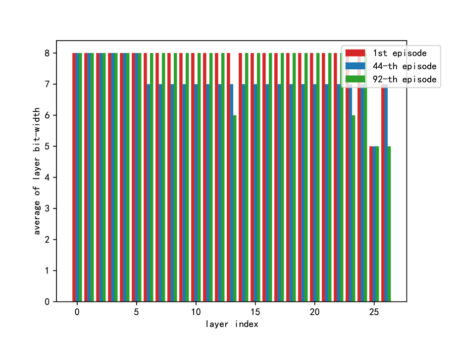
Figure 4: Quantization Plan Changes of MobileNet During Searching Under Compression Ratio = 0.2

Quantization Plan Changes During Searching: To demonstrate how AJPQ performs to some specific compression requirements, we set the compression ratio to 0.2, and performance decline should less or equal with 0 for the classification task and detection task. As shown in Figure 4, a few layers perform quantization at the beginning. To meet the compression requirement, AJPQ tends to decrease bit-width to store weights for each layer. The best quantization plan performs more quantization in the last two layers than the other layers before. Because the fully connected(FC) layers in MobileNet contains more parameters than convolution layers. As shown in Figure 5, AJPQ tends to preserve channels rather than simply pruning. Compression is less performed on the last few layers than the former layers during the searching. Because Skynet uses the final convolution layer as the detector, the last few layers may be responsible for delivering the extracted features.

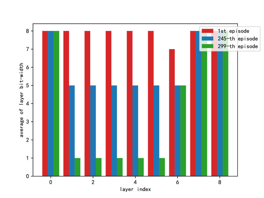
Figure 5: Quantization Plan Changes of SkyNet During Searching Under Compression Ratio = 0.2

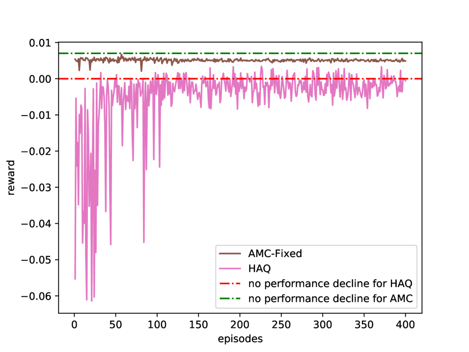
Figure 6: Rewards During Searching of AMC and HAQ Under Compression Ratio=0.2

Effectiveness evaluation of reward functions: The reward function is defined as $reward=acc(\mathcal{N}^{\prime})\times 0.01$ in AMC and $reward=(acc(\mathcal{N}^{\prime})-acc(\mathcal{N}))\times 0.1$ in HAQ , where $acc(\mathcal{N}^{\prime})$ is the performance of the compressed model and $acc(\mathcal{N})$ is the performance of the original model. The performance of those reward functions is shown in Figure 6. During the search, the AMC’s rewards are hovering below the target reward. Meanwhile, the HAQ’s rewards endure great fluctuation during the first 100 episodes. The AMC reward function gives all compression plans positive feed-backs without any discrimination. Thus, it can not efficiently explore. Meanwhile, HAQ’s reward function can distinguish the strategies that can maintain performance. However, the exploration noise of the reinforcement learning agent is not the answer to the occurrences of the vibration. The small multiplier in the HAQ’s reward function may weaken the punishment effect of negative reward. Our reward function can filter the unqualified searching strategies. As shown in Figure 7, the quantization plans violating the size reduction requirement are punished with a negative reward. Thus,the further explorations can focus on retaining performance.

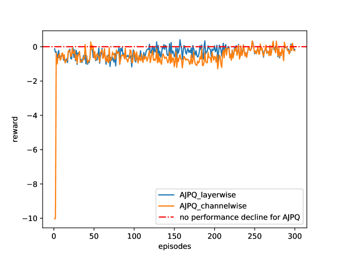
Figure 7: Rewards During Searching of AJPQ Under Compression Ratio=0.2

Conclusion

In this paper, we proposed AJPQ (Automated Model Compression by Jointly Applied Pruning and Quantization), which proved that collaborating quantization and pruning could obtain a better trade-off between the performance holding and computation reduction. After providing a new viewpoint of pruning and quantization, we proposed a hierarchical manner to perform the quantization with mixed precision. A variety of experiments demonstrated the effectiveness of the proposed joint compression. In the future, the improvement in compression plan scheduling may be achieved by hierarchical reinforcement learning (hyun Jung, won Kim, and Kim 2019).

References

- Anwar, Hwang, and Sung (2017) Anwar, S.; Hwang, K.; and Sung, W. 2017. Structured Pruning of Deep Convolutional Neural Networks. ACM Journal on Emerging Technologies in Computing Systems 13(3): 32.
- Ashok et al. (2018) Ashok, A.; Rhinehart, N.; Beainy, F.; and Kitani, K. M. 2018. N2N learning: Network to Network Compression via Policy Gradient Reinforcement Learning. In ICLR 2018 : International Conference on Learning Representations 2018.
- Bertsekas (1995) Bertsekas, D. P. 1995. Dynamic Programming and Optimal Control .
- Chen, Emer, and Sze (2017) Chen, Y.-H.; Emer, J.; and Sze, V. 2017. Eyeriss: A Spatial Architecture for Energy-Efficient Dataflow for Convolutional Neural Networks. IEEE Micro 1–1.
- Deng et al. (2009) Deng, J.; Dong, W.; Socher, R.; Li, L.-J.; Li, K.; and Fei-Fei, L. 2009. Imagenet: A large-scale hierarchical image database. In 2009 IEEE conference on computer vision and pattern recognition, 248–255. Ieee.
- Elthakeb et al. (2018) Elthakeb, A. T.; Pilligundla, P.; Mireshghallah, F.; Yazdanbakhsh, A.; Gao, S.; and Esmaeilzadeh, H. 2018. ReLeQ: An Automatic Reinforcement Learning Approach for Deep Quantization of Neural Networks. arXiv preprint arXiv:1811.01704 .
- Gao et al. (2019) Gao, X.; Zhao, Y.; Łukasz Dudziak; Mullins, R.; and zhong Xu, C. 2019. Dynamic Channel Pruning: Feature Boosting and Suppression. In ICLR 2019 : 7th International Conference on Learning Representations.
- Han, Mao, and Dally (2016) Han, S.; Mao, H.; and Dally, W. J. 2016. Deep Compression: Compressing Deep Neural Networks with Pruning, Trained Quantization and Huffman Coding. In ICLR 2016 : International Conference on Learning Representations 2016.
- Han et al. (2015) Han, S.; Pool, J.; Tran, J.; and Dally, W. J. 2015. Learning both weights and connections for efficient neural networks. In NIPS’15 Proceedings of the 28th International Conference on Neural Information Processing Systems - Volume 1, 1135–1143.
- He et al. (2018) He, Y.; Lin, J.; Liu, Z.; Wang, H.; Li, L.-J.; and Han, S. 2018. AMC: AutoML for Model Compression and Acceleration on Mobile Devices. In Proceedings of the European Conference on Computer Vision (ECCV), 815–832.
- He et al. (2019) He, Y.; Liu, P.; Wang, Z.; Hu, Z.; and Yang, Y. 2019. Filter Pruning via Geometric Median for Deep Convolutional Neural Networks Acceleration. In 2019 IEEE/CVF Conference on Computer Vision and Pattern Recognition (CVPR), 4340–4349.
- Hinton, Vinyals, and Dean (2015) Hinton, G. E.; Vinyals, O.; and Dean, J. 2015. Distilling the Knowledge in a Neural Network. arXiv preprint arXiv:1503.02531 .
- Howard et al. (2017) Howard, A. G.; Zhu, M.; Chen, B.; Kalenichenko, D.; Wang, W.; Weyand, T.; Andreetto, M.; and Adam, H. 2017. MobileNets: Efficient Convolutional Neural Networks for Mobile Vision Applications. arXiv preprint arXiv:1704.04861 .
- hyun Jung, won Kim, and Kim (2019) hyun Jung, T.; won Kim, S.; and Kim, K. 2019. N-DQN: Study on the Implementation and Research of Hierarchical Parallel Reinforcement Learning Model. The Journal of Korean Institute of Communications and Information Sciences 44(10): 1961–1974.
- Li et al. (2017) Li, H.; Kadav, A.; Durdanovic, I.; Samet, H.; and Graf, H. P. 2017. Pruning Filters for Efficient ConvNets. In ICLR 2017 : International Conference on Learning Representations 2017.
- Liu et al. (2019) Liu, Z.; Mu, H.; Zhang, X.; Guo, Z.; Yang, X.; Cheng, K.-T.; and Sun, J. 2019. MetaPruning: Meta Learning for Automatic Neural Network Channel Pruning. In 2019 IEEE/CVF International Conference on Computer Vision (ICCV), 3295–3304.
- Luo, Wu, and Lin (2017) Luo, J.-H.; Wu, J.; and Lin, W. 2017. ThiNet: A Filter Level Pruning Method for Deep Neural Network Compression. In 2017 IEEE International Conference on Computer Vision (ICCV), 5068–5076.
- Macqueen (1967) Macqueen, J. B. 1967. Some methods for classification and analysis of multivariate observations. Proceedings of the Fifth Berkeley Symposium on Mathematical Statistics and Probability, Volume 1: Statistics 1: 281–297.
- Manessi et al. (2018) Manessi, F.; Rozza, A.; Bianco, S.; Napoletano, P.; and Schettini, R. 2018. Automated Pruning for Deep Neural Network Compression. In 2018 24th International Conference on Pattern Recognition (ICPR), 657–664.
- Rastegari et al. (2016) Rastegari, M.; Ordonez, V.; Redmon, J.; and Farhadi, A. 2016. XNOR-Net: ImageNet Classification Using Binary Convolutional Neural Networks. In European Conference on Computer Vision, 525–542.
- Silver et al. (2014) Silver, D.; Lever, G.; Heess, N.; Degris, T.; Wierstra, D.; and Riedmiller, M. 2014. Deterministic Policy Gradient Algorithms. In Proceedings of The 31st International Conference on Machine Learning, 387–395.
- Wang et al. (2019) Wang, K.; Liu, Z.; Lin, Y.; Lin, J.; and Han, S. 2019. HAQ: Hardware-Aware Automated Quantization With Mixed Precision. In 2019 IEEE/CVF Conference on Computer Vision and Pattern Recognition (CVPR), 8612–8620.
- Wen et al. (2016) Wen, W.; Wu, C.; Wang, Y.; Chen, Y.; and Li, H. 2016. Learning Structured Sparsity in Deep Neural Networks. In Proceedings of the 30th International Conference on Neural Information Processing Systems, 2074–2082.
- Ye et al. (2018) Ye, J.; Lu, X.; Lin, Z.; and Wang, J. Z. 2018. Rethinking the Smaller-Norm-Less-Informative Assumption in Channel Pruning of Convolution Layers. In ICLR 2018 : International Conference on Learning Representations 2018.
- Zhang et al. (2020) Zhang, X.; Lu, H.; Hao, C.; Li, J.; Cheng, B.; Li, Y.; Rupnow, K.; Xiong, J.; Huang, T.; Shi, H.; Hwu, W.-m.; and Chen, D. 2020. SkyNet: a hardware-efficient method for object detection and tracking on embedded systems. In Conference on Machine Learning and Systems (MLSys).
- Zhu and Gupta (2018) Zhu, M. H.; and Gupta, S. 2018. To Prune, or Not to Prune: Exploring the Efficacy of Pruning for Model Compression. In ICLR 2018 : International Conference on Learning Representations 2018.
- Zhuang et al. (2018) Zhuang, Z.; Tan, M.; Zhuang, B.; Liu, J.; Guo, Y.; Wu, Q.; Huang, J.; and Zhu, J. 2018. Discrimination-aware Channel Pruning for Deep Neural Networks. In NIPS 2018: The 32nd Annual Conference on Neural Information Processing Systems, 883–894.
- Zoph and Le (2017) Zoph, B.; and Le, Q. 2017. Neural Architecture Search with Reinforcement Learning. In ICLR 2017 : International Conference on Learning Representations 2017.
- Zou et al. (2019) Zou, Z.; Shi, Z.; Guo, Y.; and Ye, J. 2019. Object Detection in 20 Years: A Survey. arXiv preprint arXiv:1905.05055 .