Theoretical survey of unconventional quantum annealing methods applied to a difficult trial problem

Abstract

We consider a range of unconventional modifications to Quantum Annealing (QA), applied to an artificial trial problem with continuously tunable difficulty. In this problem, inspired by ”transverse field chaos” in larger systems, classical and quantum methods are steered toward a false local minimum. To go from this local minimum to the global minimum, all N spins must flip, making this problem exponentially difficult to solve. We numerically study this problem by using a variety of new methods from the literature: inhomogeneous driving, adding transverse couplers, and other types of coherent oscillations in the transverse field terms (collectively known as RFQA). We show that all of these methods improve the scaling of the time to solution (relative to the standard uniform sweep evolution) in at least some regimes. Comparison of these methods could help identify promising paths towards a demonstrable quantum speedup over classical algorithms in solving some realistic problems with near-term quantum annealing hardware.

I Introduction

Quantum Annealing (QA) Finnila ; Kadowaki ; Das ; Johnson2011 ; Somma2012 ; Albash2016 is a promising method to solve optimization problems with noisy quantum hardware, with applications in machine learning, artificial intelligence Boixo2014 ; Gili ; Neukart ; Venturelli_2018 ; King2018 ; Venturelli2019 , and many other topics. The time-dependent Hamiltonian of QA is engineered to encode the solutions of classical optimization problems in its ground state. By initializing the system in the ground state of a trivial driver Hamiltonian and evolving the system sufficiently slowly, QA can find the ground state of the target (classical) problem Hamiltonian. However, it is notoriously difficult to predict the performance of QA for realistic problems. Conclusive proof of a quantum speedup over classical methods for real problems remains elusive, with the possible exception of a frustrated magnet systems king2019scaling , where an empirical scaling advantage over classical path-integral Quantum Monte Carlo (QMC) algorithms was shown. To help address this challenge, in this paper we theoretically survey a range of promising extensions to QA applied to a difficult trial problem, and identify a number of potential routes to a quantum speedup.

In the setup for QA, the total Hamiltonian in the standard uniform sweep evolution is a combination of a driving Hamiltonian $H_{0}$ and problem Hamiltonian $H_{p}$,

$$H(t)=(1-s(t))H_{0}+s(t)H_{p}$$ (1)

with the ground state of $H_{0}$ being easy to prepare. $H_{0}$ and $H_{p}$ do not commute and the time-dependent annealing parameter $s(t)$ controls the time evolution of the system. The standard uniform sweep starts from $s(0)=0$ and ends with $s(t_{f})=1$. Different functional choices for $s(t)$ may vary the efficiency of finding the ground state, such as a ‘reverse annealing schedule’ James . It’s intuitive to see that slowing down the annealing process in the vicinity of minimum gap can help increase the success probability, and this tuning is required to recover the quantum speedup in the QA formulation of Grover’s search problem Roland . However, the instantaneous minimum gap value and location is not knowable in most realistic problems, and such fine tuning is often frustrated by noise, so we will study the simplest form, a linear schedule, $s(t)$: $s(t)=\frac{t}{t_{f}}$ throughout this paper.

In QA, the ground state of a problem Hamiltonian, $H_{p}$, encodes the optimization problem solution. Experimentally realistic formulations of quantum annealing are typically arranged to solve quadratic unconstrained binary optimization (QUBO) problems, where the problem Hamiltonian is given by the Ising model,

$$H_{\mathrm{ising}}=\sum_{<i,j>}J_{ij}\sigma_{i}^{z}\sigma_{j}^{z}+\sum_{i=1}^{N}h_{i}\sigma_{i}^{z}$$ (2)

the ground state of which can be encoded as the solution space of some NP-hard problems Lucas , and given enough additional qubits, any NP complete problem can be expressed in this form. To find the ground state of the problem Hamiltonian, we first prepare the system in the ground state of $H_{0}$, which is chosen as a uniform transverse field Hamiltonian,

$$H_{0}=-\sum_{i=1}^{N}\sigma_{i}^{x}.$$ (3)

The initial ground state is a uniform superposition state in the computational basis. The quantum adiabatic theorem states that as long as the annealing evolution is slow enough, the system remains in the instantaneous eigenstate of the time-dependent Hamiltonian at all times. This theorem also provides a widely used criterion that, with the linear annealing schedule, the total adiabatic evolution time $t_{f}$ to find the ground state with high probability has an inverse minimum gap squared dependence,

$$t_{f}\propto\frac{W}{\Delta_{min}^{2}}.$$ (4)

Here, $\Delta_{min}$ is the minimum energy gap, $W$ scales as the total energy change of the final ground state $\ket{0}$ over the entire evolution: $W\sim\bra{0}H_{0}\ket{0}-\bra{0}H_{p}\ket{0}$. Note that this result is a worst case scaling estimate of the time to solution, and a variety of diabatic effects can substantially increase performance–we will encounter a number of examples of this later in this work.

In cases where the system undergoes a first order transition jorg2010energy , $\Delta_{min}$ typically decreases exponentially with the system size $N$, and the corresponding evolution time $t_{f}$ (and thus, time to solution) grows exponentially. For hard optimization problems which suffer from such phase transitions, many new schemes have been proposed to accelerate QA, such as the use of non-stoquastic Hamiltonians farhi2002quantum ; Seki ; Elizabeth ; Seki_2015 ; nishimori2017exponential ; Hormozi , inhomogeneous driving of the transverse field Susa2018a ; susa2018quantum , and oscillatory transverse fields (RFQA) Kapit2017 . We study a range of examples drawn from these works.

To investigate a number of new methods from the literature, we make our own artificially difficult problem Hamiltonian, partially inspired by previous studies of “spike problems” farhi2002quantum ; kong2015performance , rather than studying QUBO problems directly as was done in Elizabeth . In this problem, which we call the Asymmetric Magnetization Problem (AMP), local searches and QA steer the system toward a false minimum. This ‘wrong way steering’ makes finding the true ground state exponentially difficult. The difficulty exponent associated with the AMP can be continuously tuned for further investigation of the performance of these alternative QA methods with problem hardness. Further, the energy landscape depends only on total magnetization $m$, making it easier to study analytically. We do not consider noise in this paper, as none of the methods we consider require fine tuning. We expect these methods to be resilient to noise described by the empirical noise model for superconducting flux qubits. There is strong theoretical evidence for this resiliency in the case of RFQA Kapit2017 , and both theoretical and experimental evidence for inhomogeneous driving Berry2009 ; Susa2018a ; susa2018quantum ; adame2020 .

The rest of the paper is organized as follows. In Section II, we introduce our trial problem; in Section III, we provide an analytical prediction of its minimum gap. Section IV discusses the performance of the standard uniform sweep applied to this problem, against which we benchmark all other methods. We then introduce inhomogenous driving, transverse couplers and RFQA, comparing their behavior with the standard uniform sweep routine in Sections V and Section VI separately. The final section summarizes our results and provides comments on the performance of these methods.

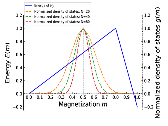
Figure 1: Density of states distribution and energy of the problem Hamiltonian in the AMP model. The x axis is the total magnetization $m$, the y axis represents both the energy spectrum of the problem Hamiltonian(left) and the density of states distribution(right). The dashed lines are the density of states for system sizes of N=10, 11, 12. The distributions become narrower with increasing system size. The solid blue line is the energy landscape of $H_{p}$. In our model, the distribution follows a Gaussian distribution, centered at $m=0.5$. Comparing the distribution of density of states with the energy spectrum of the problem Hamiltonian, we see the peaks of the density of states are distributed behind the global maximum. The asymmetry of the $H_{p}$ results in an exponentially difficult problem.

II Asymmetric Magnetization Problem

While conventional Ising Hamiltonians can encode nearly any combinatorial optimization problem, we choose an artificial toy problem model to better study a variety of new methods to find its solution. This is in part because extracting exponential difficulty scaling is notoriously difficult and unreliable in random structured problems, at least when $N$ is small enough for exact classical simulation. Our artificial problem, the “AMP”, has the problem Hamiltonian defined as function of total magnetization $m$,

$$H_{p}=f(m);\;\;m=\frac{1}{2N}\sum_{i=1}^{N}(1+\sigma_{i}^{z})$$ (5)

where N is the system size, $\sigma_{i}^{z}$ is the Pauli matrix with discrete eigenvalues $\pm 1$, $f(m)$ is designed to have two competing ground states at $m=0$ and $m=1$ with all spins down and all spins up. The form of $f(m)$ is controlled by two free parameters, $A$ and $x_{p}$:

$$f(x)=\begin{cases}\frac{x}{x_{p}}&\text{if $x<x_{p}$}\\ 1-(1+A)\frac{x-x_{p}}{1-x_{p}}&\text{if $x\geq x_{p}$}\\ \end{cases}$$ (6)

Here, $f(1)$ is the true ground state, and $f(0)$ is the false minimum. $x_{p}$ defines the location of the global maximum, and $A$ defines the energy difference of the two competing states: $f(0)-f(1)=A$. By adjusting these two parameters, we can continuously tune the difficulty of the problem.

The difficulty of finding the global minimum in our model is strongly related to the distribution of the density of states. The density of states follows a Gaussian distribution as shown in FIG. 1, with the most probable initial state centered at $m=0.5$ where half of the spins are flipped from the true ground state, and a global maximum is distributed at $m=x_{p}>0.5$. We see the system has a large tendency to get stuck in the local minimum, since the possible initial state is settled behind the global maximum. The wrong way guidance is the generic failure mechanism for classical and quantum optimization algorithms Albash2 , as if local guidance from a random initial state tends to point toward the true solution of a problem it can be solved trivially. But if local guidance points toward false minima, then the problem can quickly become hard, and in more realistic problems at large $N$ there are often exponentially many local minima. Multiqubit tunneling between well-separated minima–exactly the process we simulate here–has been identified as a critical bottleneck in many realistic problems  knysh2016 .

In the AMP problem, we set the global maximum at $m=x_{p}$ where $x_{p}>0.5$, with two competing ground states at each end. From the density of states distribution in FIG. 1, we can tell the system has a large tendency to be steered toward the false minimum. In classical algorithms such as simulated annealing, the system will easily get stuck in the false minimum since the possible initial state is mostly distributed around $m=0.5$. The possibility of finding the global minimum is large if the initial instantaneous state of $H_{p}$ happens to be guessed beyond the global maximum at a position that $m>x_{p}$, but if the initial state is located at any $m<x_{p}$, the possibility of climbing the hill is exponentially small. Cost functions similar to the AMP model have been studied in farhi2002quantum ; kong2015performance , and classical simulated annealing was shown to be inefficient for solving such problems. We will show that the AMP problem is also exponentially difficult to solve with quantum annealing, and we focus on how various modifications to QA compare with a homogeneous transverse field and uniform sweep (the “default” quantum annealing method) in solving the AMP problem.

When applying QA to the AMP problem, performance is bottlenecked by an exponentially small gap at a first-order transition jorg2010energy ; Bibes2010 ; Laumann . As shown in FIG. 4, the magnetization is entropically steered toward 0 as the system evolves, and all $N$ spins must simultaneously flip to reach the true ground state. The difficulty scaling of the problem model can be tuned by $A$ and $x_{p}$; smaller $A$ corresponds to a smaller energy gap between the two competing ground states, which intuitively increases the difficulty level of the problem. Similarly, larger $x_{p}$ moves the peak further away from the center of the density of states, and the system then has larger tendency to be steered to the false local minimum, which also increases problem difficulty. We make an ensemble of problem models with different $A$ and $x_{p}$ so that we can investigate the relationship between the performance of different methods with the difficulty of the problem models. We make modifications to the traditional QA method and evaluate their performance by numerically calculating the time to solution, and show that the AMP problem is exponentially difficult to solve with quantum algorithms, but modifications to the traditional QA method can lead to substantial improvements in the scaling of the time to solution. The exponential scaling coefficients for each method are listed in Table I.

Although this toy model is just a simplified artificial problem without a realistic implementation, as described above, it captures the basic bottleneck of most classical and quantum optimization problems. So any method which accelerates finding a solution in the AMP is likely broadly applicable to more realistic cases.

III Analytical prediction of the minimum gap

The minimum gap $\Delta_{min}$ determines the worst case difficulty of a problem, so analytically predicting it can help us to better assess the behavior of quantum annealing algorithm. To compute it, we use a modified form of the “forward approximation” $N$th order perturbation theory employed in pietracaprina2016forward ; baldwinlaumann2016 ; baldwinlaumann2017 ; scardicchio2017perturbation ; baldwin2018quantum . In this approximation, the minimum gap is predicted to be

$$\Delta_{min}=N!\frac{\prod_{i=1}^{N}\kappa_{i}}{\prod_{n=1}^{N-1}U_{n}}$$ (7)

where $\kappa_{i}$ is the transverse field strength on each site $i$ (evaluated at the critical point $\kappa_{c}$), and $U_{n}^{-1}$ is the average of the inverse of the energy difference to flip $n$ spins from either ground state

$$\frac{1}{U_{n}}=\Bigg{\langle}\frac{1}{\epsilon_{n}+\delta_{\epsilon_{n}}-\epsilon_{0}-\delta_{\epsilon_{0}}}\bigg{\rangle}.$$ (8)

Here, the $\epsilon$ terms are the classical energies defined in the problem Hamiltonian and the $\delta$ terms are their perturbative corrections from the transverse field, which act to increase the excitation energies in this case. Including these corrections in the energy denominators (which is effectively a resummation scheme) is vital to obtaining relatively accurate predictions; explicitly, for the AMP

$$U_{n} \simeq n\left(\frac{1}{x_{p}}+2\kappa_{c}^{2}x_{p}\right),\;\;\;\left\{n\leq x_{p}N\right\},$$

$$\simeq \left(N-n\right)\left(\frac{1+A}{1-x_{p}}+2\kappa_{c}^{2}\frac{1-x_{p}}{1+A}\right)\;\;\;\left\{n>x_{p}N\right\}.$$

From this expression, it is straightforward to predict the minimum gap in our problem. As shown in FIG. 2, the exponential fitting of numerical $\Delta_{min}$ as a function of $N$ for descending difficulty problem sets are: $2^{-0.4-1.12N}$, $2^{-0.79-0.74N}$, $2^{-1.35-0.52N}$, $2^{-2.04-0.31N}$. FIG. 3 indicates that the scaling of our theoretical prediction matches well with the numerical result by multiplying by a factor of $2\pi/N$. Eq.(7) appears to overestimate the true gap by a factor of $\sim N/2\pi$; the reason for this is unclear. Some level of disagreement is expected, however, particularly in the easiest difficulty parameter set. If the coefficient of the problem Hamiltonian is 1, the phase transition for those parameters occurs at $\kappa_{c}\simeq 1.73$. At such a large value of $\kappa_{c}$ the ratio of $\kappa$ to the single spin excitation energy approaches unity and thus a perturbative expansion in it may break down.

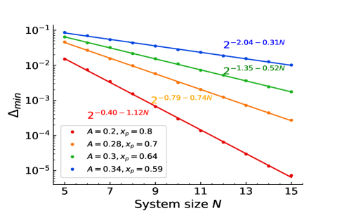
Figure 2: Numerical values of the minimum gap for four parameter sets, with the system size $N$ ranging from 5 to 12 spins. The points are data of numerically estimated minimum gap energies, least squares fits of the minimum gap are red, orange, green and blue solid lines. The minimum gaps in the four problem sets all decrease exponentially with increasing system size.

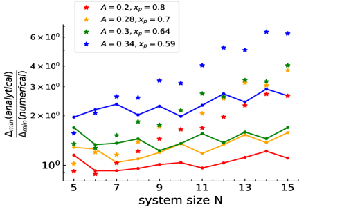
Figure 3: Ratio of analytical and numerical values of minimum gap in four problem sets, system size $N$ ranging from 5 to 12. The analytical values of $\Delta_{min}$ are from the modified forward approximation (Eqs.(7 – III)). Star marker represents the ratio of analytical and numerical values of minimum gap, dot-line represents the ratio of analytical and numerical values with a correction term $2\pi/N$. The corrected analytical predictions in the four sets match well with the numerical values.

IV Standard uniform sweep routine

We first investigate the performance of the standard uniform sweep method, for system sizes $N$ ranging from 5 to 18 spins. In this method, the driving Hamiltonian is a homogeneous transverse field: $H_{0}=-\sum_{i=1}^{N}\sigma_{i}^{x}$. The total Hamiltonian is a combination of the drive Hamiltonian and problem Hamiltonian $H_{p}$

$$H(s)=-(1-s)\frac{1}{N}\sum_{i=1}^{N}\sigma_{i}^{x}+sH_{p}.$$ (10)

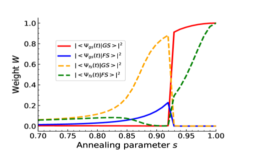
Figure 4: The instantaneous overlap of the ground and first excited states with the true and false ground states of the classical problem as a function of the annealing parameter $s$, with system size $N=8$, and the problem Hamiltonian is defined with parameters: $A=0.2,x_{p}=0.8$. The x axis is the annealing parameter $s$ in a small range from 0.7 to 1, the y axis denotes the probability of getting a specific state. The red and blue solid lines are the overlap of the instantaneous ground state with the true and false ground state of $H_{p}$, the orange and green dashed lines are the overlap of the instantaneous first excited state with the true and false ground state of $H_{p}$. The comparison shows that the system is steered toward the false minimum first and all N spins have to flip to reach the true ground state.

The initial ground state of the system is the ground state of $H_{0}$, which is a uniform superposition of states corresponding to all possible assignments of bit values with equal weights. As the system evolves, the Hamiltonian linearly interpolates between the transverse field Hamiltonian and the problem Hamiltonian, i.e. starting as $H_{0}$ and ending in $H_{p}$. As long as the system stays in the instantaneous ground state, the system will be steered toward the false minimum first, but at some critical $s_{c}$ the true and false ground states cross and all $N$ spins must flip, as shown in FIG. 4 with red and blue solid lines. For this problem, there is only one avoided crossing in the standard uniform sweep method (though we find multiple crossings when inhomogenous driving is employed). Since the gap at the phase transition point is exponentially small in $N$, unless the evolution is performed extremely slowly, the avoided crossing will be diabatically missed and the probability of finding the true ground state will be suppressed, while the probability of finding the false ground state dominates, as shown in FIG. 4 with orange and green dashed lines.

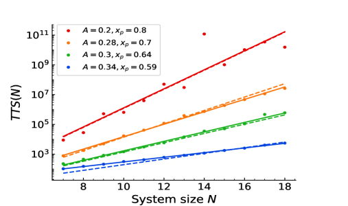
Figure 5: Time to solution to find the true ground state in four problem model sets using the standard uniform sweep method, computed from the final success probability for a runtime polynomially increasing with $N$. The difficulty level of the four models is arranged in descending order: $\{A=0.2,x_{p}=0.8\}$; $\{A=0.28,x_{p}=0.7\}$; $\{A=0.3,x_{p}=0.64\}$; $\{A=0.34,x_{p}=0.59\}$. Dots are data with the standard uniform sweep method, solid lines are best-fit curves of the numerical data and dashed lines are the inverse of the square of the numerically estimated minimum gap from FIG. 2. The time to solution closely tracks the average minimum gap squared as expected. In all cases, the $N$-spin tunneling bottleneck in this problem leads to an exponentially increasing time to solution.

We evaluate the performance of the standard uniform sweep algorithm by computing the time to solution($TTS$) over a range of system sizes. The $TTS$ measures the time needed to find the ground state with $99\%$ success probability Albash2

$$TTS\propto t_{f}\frac{\ln(1-0.99)}{\ln(1-p(t_{f}))},$$ (11)

where $p(t_{f})$ is the success probability in a single-trial with runtime $t_{f}$; for small $p(t_{f})$, $TTS\propto t_{f}/p(t_{f})$. As mentioned in the introduction, the evolution time needed to find the ground state increases as $\Delta_{min}^{-2}$. To explore the performance of the standard uniform sweep method under different problem models, we choose four sets of parameters: $\{A=0.2,x_{p}=0.8\}$; $\{A=0.28,x_{p}=0.7\}$; $\{A=0.3,x_{p}=0.64\}$; $\{A=0.34,x_{p}=0.59\}$ forming an ensemble of problem models with descending difficulty level. These parameters are chosen to approximately set $\Delta_{min}\propto\left\{2^{-N},2^{-3N/4},2^{-N/2},2^{-N/4}\right\}$, respectively. As mentioned previously, increasing $A$ or decreasing $x_{p}$ toward $1/2$ both decrease the difficulty exponent, and moving either parameter in the opposite direction makes the problem harder.

As expected by an exponentially closing gap, the time needed to find the solution exponentially increases with system size. This is confirmed in FIG. 5, where the corresponding time to solution exponentially increases with the system size in all problem sets, and the difficulties of the four sets are well separated from each other. With the minimum gap and performance of the standard uniform sweep method rigorously understood, we now apply other methods from the literature to compare their performance with it and investigate their abilities of providing a quantum speedup.

Problem set	$1/\Delta_{min}^{2}$	$S$	$I$	$C_{F,A,M}$	$M$	$CM$	$SyncM$	$SyncMC$	$D$
$A$=0.2,$x_{p}$=0.8	2.25	2.12	0.79	1.77, 2.09, 2.50	1.48	1.31	1.28	0.86	1.56
$A$=0.28,$x_{p}$=0.7	1.48	1.39	0.70	1.25, 1.23, 1.67	0.89	0.86	0.84	0.64	1.05
$A$=0.3,$x_{p}$=0.64	1.04	1.06	0.69	0.87, 0.77, 1.12	0.62	0.62	0.64	0.62	0.50
$A$=0.34,$x_{p}$=0.59	0.61	0.52	0.69	0.48, 0.44, 0.54	0.45	0.45	0.45	0.51	0.40

Table 1: Summary of scaling exponents for each method. Fitting the time to solution $TTS(N)$ of each method to $2^{\beta+\gamma N}$, the table lists the exponential scaling coefficient “$\gamma$” value for each method. “$S$” represents the standard uniform sweep method, “$I$” represents the Inhomogeneous driving method, “$C_{F,A,M}$” represents the transverse couplers method, in which “F,A,M” corresponds to ferromagnetic, anti-ferromagnetic, mixed couplers, respectively. “$M$” represents the RFQA-M method, “$CM$”, RFQA-M with couplers method, “$SyncM$”, synchronized RFQA-M method, “$SyncMC$”, synchronized RFQA-M with couplers method, and “$D$” represents the RQFA-D method.

V summary of results

Before we proceed to the detailed investigation of alternative QA methods, we compile a summary in TABLE.1, that lists the exponential fitting results of $TTS$ for each method. We fit $TTS(N)$ to $2^{\beta+\gamma N}$ and extract the “$\gamma$” value to determine the difficulty scaling for each method. We find that in the harder problem sets where ${x_{p}=0.8,A=0.2}$ and ${x_{p}=0.7,A=0.28}$, synchronized RFQA-M (with transverse couplers) and Inhomogeneous driving show the best performance, but in the relatively easier problem sets where ${x_{p}=0.64,A=0.3}$ and ${x_{p}=0.59,A=0.34}$, the RFQA-D method shows the best scaling advantage. The details are illustrated and discussed in the following sections; we include this table as a central reference point for the results of all of our studies.

VI Modified Adiabatic annealing strategies: inhomogenous driving and transverse couplers

A wide range of modifications to quantum annealing have shown significant promise in theoretical studies Seki ; Elizabeth ; Hormozi ; SelsE3909 ; vinci2017non ; Marshall2018 ; susa2018quantum ; Gra ; Hauke_2020 . In this section, we begin applying methods from the literature to our AMP model and assess their performance by computing the $TTS$ as in Eq. 11. We begin by considering inhomogeneous driving method and transverse couplers. Inhomogeneous driving and the ferromagnetic transverse couplers belong to the class of stoquastic Hamiltonians, while the anti-ferromagnetic couplers and mixed-sign couplers have non-stoquastic Hamiltonians. A stoquastic Hamiltonian has real and non-positive off-diagonal matrix elements in the computational basis Sergey , and can often (but not always  Evgeny ) be efficiently simulated by sign-problem-free quantum Monte Carlo (QMC). Non-stoquastic Hamiltonians, on the other hand, suffer from a sign problem and thus cannot be efficiently simulated in QMC in general, though some particular non-stoquastic Hamiltonians can be simulated in QMC by clever schemes to avoid the sign problem Ohzeki2017 . Amenability (or not) to QMC is a critical issue in QA, as in recent studies, QMC displays comparable exponential scaling to the physical incoherent tunneling rate in quantum annealers Denchev ; Isakov ; Jiang ; Evgeny ; Mazzola . It’s thus intuitive to infer that the efficiency of QMC and quantum annealers are similar in solving many problems, making it difficult to realize a genuine quantum speedup. Non-stoquastic Hamiltonians do not suffer from this issue, and have demonstrated significant benefits in some theoretical work Seki ; Seki_2015 ; Nishimori ; susa2017relation ; Hormozi .

VI.1 Inhomogeneous driving

In inhomogeneous driving, the transverse fields are ramped down at different rates from one site to the next, as first described in Susa2018a ; susa2018quantum . In the original proposal  Susa2018a , the magnitude of the transverse field applied to the $N$ spins is turned off sequentially with a set of time-dependent amplitudes $\Gamma_{i}(s)$. In that work, the inhomogeneous driving transverse field circumvents the first-order quantum phase transition and provides an exponential quantum speedup in a p-body interacting mean-field-type model. A more careful analysis susa2018quantum which included noise and disorder found the exponential speedup to be somewhat fragile, but showed that a consistent polynomial speedup persisted given these more realistic assumptions. Further, there is experimental evidence that inhomogenous driving is effective in real hardware  adame2020 .

Inspired by the performance improvements offered by inhomogeneous driving of the transverse field Hamiltonian, we apply it to the four AMP problem sets as follows

$$\begin{split}&H(t)=-\frac{1}{N}\sum_{i=1}^{N}\Gamma_{i}(s)\sigma_{i}^{x}+sH_{p},\\ &\Gamma_{i}(s)=\begin{cases}1&\text{if $s<s_{i}$}\\ N(1-s^{r})+(1-i)&\text{if $s_{i}\leq s\leq s_{i-1}$}\\ 0&\text{if $s_{i-1}<s$}\\ \end{cases}\end{split}$$ (12)

Interestingly, the measurement of $TTS$ in FIG. 6 shows that the inhomogeneous driving method has a difficulty scaling which is very weakly dependent on the control parameters $A$ and $x_{p}$, with the $TTS$ scaling virtually identically in each case. It consequently outperforms the standard uniform sweep method for the harder problem regimes, but actually shows worse performance for the easiest parameter sets. While we cannot predict its performance analytically in this case (the perturbation theory we use to calculate $\Delta_{min}$ is not well defined for some of the transverse fields set equal to strictly zero), a clue to the origin of this behavior is found in a numerical analysis of the level structure, as we now describe.

In FIG. 7 we show the energy difference of the higher order excited states with the ground state in the hardest problem class with $N=10$. In contrast to a uniform sweep, we find two avoided crossings in the annealing process, a generic feature of inhomogenous driving in this system that we observed for other parameter sets as well (data not shown). The presence of two crossings is likely what is responsible for the performance boost observed in the harder problems, and why it seems to have the same scaling for different parameters. A similar phenomenon is observed in the glued trees problem somma2012quantum , where constructive interference of diabatically missing two avoided crossings leads to an exponential speedup. However, unlike the glued trees problem, there is no clear separation between the two competing ground states and the higher excited states in the AMP model. It is clear from FIG. 7 that there also exists an overlap region of the higher order excited states with the first excited state. As $A$ and $x_{p}$ are varied to make the difficulty scaling decrease, the two avoided crossings move closer together, and the distance from higher levels also shrinks and becomes exponentially small. Consequently, this effect does not result in an exponential speedup here, and shows worse performance than a uniform sweep in the easiest cases.

Figure 6: Time to find the true ground state in four problem model sets using the inhomogeneous driving method, computed from the final success probability for a runtime polynomially increasing with $N$. Dots are data with the inhomogeneous driving method, cross points are data with the standard uniform sweep method, dashed lines are best-fit curves of the inhomogeneous driving method, solid lines are best-fit curves of the standard uniform sweep method for comparison purpose. The inhomogeneous driving method helps in the harder cases but in the easier cases it is less efficient than the standard uniform sweep.

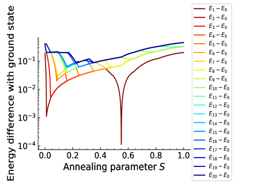
Figure 7: Energy difference of the higher order excited states with the ground state. This is the hardest problem where $\{A=0.2,x_{p}=0.8\}$, $N=10$. We simulated the energy differences up to 20th excited state.

VI.2 Transverse couplers

Adding two-body transverse coupling to QA Seki ; Seki_2015 ; susa2017relation ; Hormozi is often considered to be a promising route to a quantum speedup. For instance, Hormozi et al Hormozi , constructed a stoquastic Hamiltonian by inserting ferromagnetically coupled term $H_{I}^{F}$ to the traditional Ising model, and a non-stoquastic Hamiltonian by inserting antiferromagnetically coupled term $H_{I}^{A}$ or mixed coupled term $H_{I}^{M}$ as follows

$$H_{I}^{F}=-\sum_{i<j=1}^{N}\sigma_{i}^{x}\sigma_{j}^{x}$$ (13)

$$H_{I}^{A}=+\sum_{i<j=1}^{N}\sigma_{i}^{x}\sigma_{j}^{x}$$

$$H_{I}^{M}=\sum_{i<j=1}^{N}r_{ij}\sigma_{i}^{x}\sigma_{j}^{x}$$

$r_{ij}$ is randomly chosen from $\{-1,1\}$ to include both ferromagnetic and antiferromagnetic cases. In that work, they found that both stoquastic and non-stoquastic Hamiltonians showed an advantage over a uniform transverse field for a class of long-range Ising spin glass problems, with the non-stoquastic methods generally showing better performance. This motivated us to investigate the same method in our AMP model. We add transverse couplers into our model and choose a path of the formfarhi ; Hormozi

$$H(s)=(1-s)\frac{1}{N}H_{0}+s(1-s)\frac{1}{N}H_{I}+sH_{p}.$$ (14)

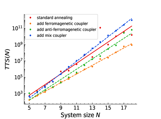
Figure 8: Time to find the true ground state in the hardest problem set:$\{A=0.2,x_{p}=0.8\}$ using the transverse coupler methods, computed from the final success probability for a run-time polynomially increasing with $N$. Data for adding a ferromagnetic coupler, an anti-ferromagnetic coupler, and mixed couplers are given by orange, green, blue dots, respectively. Red dots are data of the standard uniform sweep method for comparison purpose. The solid red line is the best-fit curve of the standard uniform sweep method for comparison. Other dashed lines are best-fit curves for the transverse couplers methods. Adding ferromagnetic and anti-ferromagnetic couplers to the conventional standard uniform sweep routine show obvious quantum speed up, although adding the mixed couplers reduces the advantage to some extent.

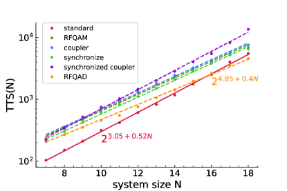
(a)

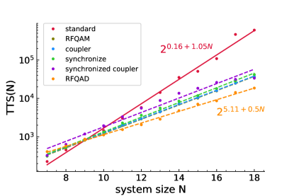
(b)

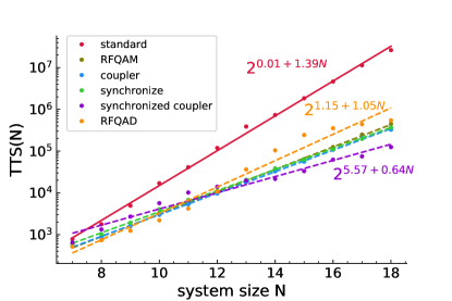
(c)

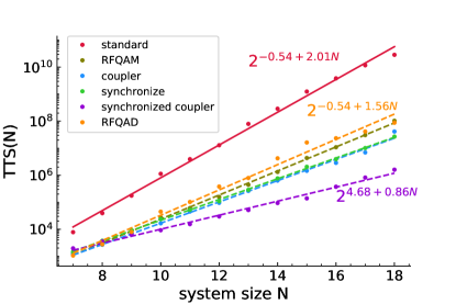
(d)

Figure 9: Time to find the true ground state in four problem model sets using the RFQA method, computed from the final success probability for a run-time polynomially increasing with $N$. Dots are data with RFQA methods, the solid red line is the best-fit curve of the standard uniform sweep method for comparison purpose. Other dashed lines are best-fit curves of the RFQA methods. RFQA methods show obvious scaling advantages over the standard quantum annealing, with generally greater relative improvements in the harder problem cases.

We apply the transverse coupler Hamiltonian to our four problem sets, plotting the results for the hardest scaling choice as an example in FIG. 8. It is straightforward to see that adding ferromagnetic or anti-ferromagnetic coupler has a clear scaling advantage over a standard uniform sweep, but mixed couplers actually lead to decreased performance. The quantum speedup from coupler terms is probably because the couplers can flip two spins simultaneously, so the tunneling process from one configuration to the other can occur at lower order than with a uniform transverse field (where it occurs at Nth order in this model). The ferromagnetic coupler increases the minimum gap and thus provides a quantum speedup over the standard uniform sweep method, the same effect is observed inHormozi . The antiferromagnetic couplers actually decreased the minimum gap but still show a scaling advantage, so the reason for the increased performance from the antiferromagnetic ones remains elusive. The behavior of the transverse coupler methods in other three problems sets are shown in TABLE I.

VII Reverse annealing and cold baths

Reverse annealing perdomo2011study ; chancellor2017modernizing ; ohkuwa2018reverse ; king2018observation , where the system is initialized in a local classical minimum and the transverse field is ramped up and down to search for other minima, unfortunately provides no benefit for the AMP. Reverse annealing was shown in ohkuwa2018reverse to provide benefit for the p-spin ferromagnet problem, if one is able to guess an initial state sufficiently close to the true ground state. However, in the AMP there are only two minima to choose from, separated by $N$ spin flips. The only sensible choice (without dramatically modifying $H_{P}$) is thus to initialize the system in the false minimum. We simulated the reverse annealing protocol (data not shown) by initializing the system in the false minimum, ramping the transverse field up to a finite value guessed randomly from an $O(1)$ range enclosing the phase transition point, evolving from that point for $O\left(N^{2}\right)$ time, then ramping it back down to zero. With sufficient averaging over the location of the pause point (which is not knowable precisely in real problems), we found a time to solution which scaled nearly identically to the standard uniform sweep method for all parameters studied. Thus, we found no benefit in applying reverse annealing to this problem.

The influence of a cold bath on this system is more subtle. It is well known keck2017dissipation ; smelyanskiy2017quantum ; venuti2017relaxation ; arceci2018optimal ; marshall2019power ; kadowaki2019experimental ; suzuki2019quantum ; roberts2019noise that coupling a quantum spin glass to a cold bath can improve the process of finding its low energy states. So let us consider coupling the AMP to a low temperature bath during annealing. Importantly, we here assume that $T$ is small compared to the single qubit excitation energy, but it may still be large compared to the (exponentially small) minimum gap. How much can such a bath improve the time to solution?

Unfortunately, numerical simulation of such a system is prohibitively expensive jaschke2019thermalization given the complexity of the Lindblad operators used to represent the finite temperature bath. We can however estimate the relaxation rate from the bath by appealing to the MSCALE conjecture Kapit2017 . This conjecture states that, for few-body operators, the scaling (with problem size $N$) of matrix elements of these operators between competing ground states of quantum spin glasses near a phase transition is the same as the scaling of the minimum gap itself. This conjecture is true by inspection for the AMP, since the gap can be computed accurately using the modified forward approximation in Sec. III. If we assume that each spin couples to a cold bath independently, then the rate of mixing near the phase transition scales as $N\Gamma_{B}^{2}/W$ , where $\Gamma_{B}\propto\Delta_{\rm min}$ is the matrix element from a local spin operator and $W$ is the energy range swept over. This produces a factor of $N$ enhancement relative to the closed system, but does not change the scaling exponent as the other methods do. The cold bath may however improve performance in a real system by relaxing few-body excitations back toward the ground state, correcting “errors” induced by other channels.

VIII RFQA

Stoquastic or not, the previous sections all explored “DC” schemes involving slow variations of transverse field and coupler terms. In this section, we consider an AC alternative, called RFQA Kapit2017 . In RFQA, the traditional transverse field driver Hamiltonian is modified by independently oscillating either the magnitude (RFQA-M) or direction (RFQA-D) of each transverse field term (M and D refer to magnitude and direction, respectively). As we will describe shortly, the qualitative explanation for a quantum speedup in RFQA is an exponential proliferation of weak many-spin processes, leading to accelerated mixing near first order quantum phase transitions. The total Hamiltonian in RFQA is given by

$$H(t)=(1-s)H_{M/D}(t)+sH_{p},$$ (15)

where the driving fields in RFQA-M and RFQA-D are defined as follows

$$\begin{split}&H_{M}(t)=-\kappa\sum_{i=1}^{N}(1+\bar{\alpha_{i}}\sin(2\pi f_{i}t))\sigma_{i}^{x},\\ &H_{D}(t)=-\kappa\sum_{i=1}^{N}[\cos(\bar{\alpha_{i}}\sin(2\pi f_{i}t))\sigma_{i}^{x}+\\ &\ \ \ \ \ \ \ \ \ \ \ \ \sin(\bar{\alpha_{i}}\sin(2\pi f_{i}t))\sigma_{i}^{y}].\end{split}$$ (16)

Here, $\bar{\alpha_{i}}$ is the amplitude of each oscillation, the frequencies $f_{i}$ of the field are randomly chosen between $f_{min}$ and $f_{max}$, and $\kappa$ is the magnitude of the transverse field. To avoid uncontrolled heating, both $f_{min}$ and $f_{max}$ have inverse polynomial scaling in N. To estimate the performance of RFQA, we average the success probability $p(t_{f})$ over hundreds of random choices of the $\{f_{i}\}$ when computing time to solution. The RFQA methods all rely on finite frequency dynamics that are not captured by QMC, making them promising candidates for producing a quantum speedup. The two methods are straightforward to implement in flux qubit hardware, by applying oscillating magnetic fields as described in Kapit2017 .

As described in the original work, the qualitative speedup mechanism from RFQA is complex and arises from an exponential proliferation of weak multi-photon transitions. As the system nears a phase transition point, whenever the energy of the two ground states crosses a combination of $m$ oscillating frequencies there is an $m$th order driving process that (very weakly) mixes the two states. In general, the Rabi frequency of such a process decreases exponentially in $m$, but there are $2^{m}\binom{N}{m}$ such terms and the combination of all of them dramatically accelerates the phase transition. If the $m$th order resonance is smaller than the base tunneling rate $\Omega_{0}=\Delta_{min}/2$ by a factor $\Lambda^{m}$, then the total transition rate is expected to scale approximately as

$$\Gamma_{T} = \frac{\sum_{i=1}^{N}|\Omega_{i}|^{2}}{W}\simeq\frac{\Omega_{0}^{2}}{W}\sum_{l=1}^{N}\Lambda^{2l}{N\choose l}2^{l}$$

$$\simeq \frac{\Omega_{0}^{2}}{W}\left(1+2\Lambda^{2}\right)^{N}.$$

Predicting $\Lambda$ is a subtle challenge and something we will leave for future work; we restrict our study of RFQA to purely numerical simulations here.

VIII.1 RFQA-M

In RFQA-M the magnitudes of the transverse field terms coherently oscillate with time as the global amplitude is ramped down toward 0, so that an individual transverse field term $\kappa$ is replaced with $\kappa\left(1+\bar{\alpha}\sin 2\pi f_{i}t\right)$. In our simulations we used $\bar{\alpha}=0.9$, and magnitude of frequencies $f_{i}$ is randomly chosen between $\{\frac{0.01}{N^{1.5}},\frac{0.02}{N{1.5}}\}$; the signs of the $f_{i}$ are also randomly chosen. This is superficially similar to inhomogenous driving, but the coherent oscillations lead to non-monotonic changes of $\kappa_{i}$ with time and very different scaling as a result. We also considered a few additional variations of RFQA-M. In one set of simulations, we explored a partially synchronized RFQA-M method, in which $N$ spins are broken into $k$ groups, instead of generating different random frequencies for each site, the transverse fields in each group are all oscillated in phase with the same frequencies. In this work, we only divided the $N$ spins into two groups, but other arrangements are possible. We also explored adding ferromagnetic/antiferromagnetic couplers to the RFQA-M method, where all transverse couplers and fields are independently oscillated in magnitude. The total Hamiltonian in this method is defined as follows

$$H(s) =(1-s)H_{M/D}+sH_{p}$$ (18)

$$+(1-s)\kappa_{r}\sum_{<i,j>}\sin(2\pi r_{ij}t)\sigma_{i}^{x}\sigma_{j}^{x}$$

where $\kappa_{r}$ is the magnitude of the coupler terms, $r_{ij}$ are the oscillating frequencies of the coupler, randomly chosen between $\{r_{min},r_{max}\}$. The magnitude $r$ is defined to polynomially decrease with $N$, and the frequencies $r_{ij}$ are also inverse polynomial in $N$. Finally, we looked at partially synchronized RFQA-M with transverse couplers, where the transverse couplers are also synchronized into groups.

We compare the $TTS$ of the various implementations of RFQA-M with the standard uniform sweep method in FIG. 9. The results show that RFQA-M and its adaptions can provide quantum speed up over the standard uniform sweep routine, with a scaling advantage which is particularly obvious in harder problem sets.

VIII.2 RFQA-D

In RFQA-D the direction of each transverse field term oscillates in time, tipping back and forth in the $x-y$ plane. This can be engineered through oscillating $z$ biases (which can be shown to be equivalent to a tipping transverse field through a time-dependent unitary transformation) and has the elegant property that the instantaneous spectrum of the system is preserved in the evolution, so the oscillations have no “steering” effect whatsoever (unlike RFQA-M, where changing transverse field magnitudes can change the relative energies of competing ground states, in addition to any AC effects). Any performance advantage from RFQA thus comes directly from the proliferation of weak transitions described above.

As shown in FIG. 9, we see that RFQA-D does provide an obvious quantum speed up over a uniform sweep. In all studied cases, RFQA-D reduced the exponent for $TTS(N)$ relative to the standard uniform sweep, and for the two easier difficulty regimes, it outperformed all other studied methods. We expect that these results will carry over to the larger class of optimization problems that experience wrong-way steering towards false minima.

IX Conclusion

In this work, we defined a simple toy model– the asymmetric magnetization problem– with two competing ground states separated by a global peak, and used it to benchmark a variety of modifications to quantum annealing in the literature. The problem is exponentially difficult to solve due to its exponentially closing gap, and the entropic steering toward a false minimum responsible for its difficulty is a generic bottleneck mechanism for a huge array of optimization problem classes. Thus, methods to accelerate finding the solution in it should prove beneficial in much broader contexts.

We studied an ensemble of problem model sets with descending difficulty: $\{A=0.2,x_{p}=0.8\};\{A=0.28,x_{p}=0.7\};\{A=0.3,x_{p}=0.64\};\{A=0.34,x_{p}=0.59\}$, and assessed a variety of new quantum methods by evaluating the scaling of the time to solution ($TTS$). To have a straightforward view of the performance of each method, we fit their $TTS$ to exponential functions and extracted the exponential scaling value, summarized in TABLE I. The standard uniform sweep method shows inverse gap squared dependence as expected. In contrast, in the inhomogeneous driving approach, the $TTS$ has a nearly constant difficulty scaling of $2^{\sim 7N/10}$, roughly independent of the tuning parameters. It likely means that the problem is steered less toward the false minimum in this case than it is for uniform driving, but that is not enough to avoid a first order transition and the resulting lack of guidance becomes counterproductive when the problem is easier.

While the problem we studied is homogeneous (in that energy is a function of total magnetization only), we don’t expect disorder to significantly change the results for the standard uniform sweep, couplers and RFQA. If we modeled disorder as a simple random $Z$ term with magnitude  $1/N$ for each spin (recall that the problem energy is $O\left(1\right)$) added to $H_{p}$, it would change the relative energies of the ground states by $1/\sqrt{N}$ for the energy scale we have chosen. This will move the transition point $s_{c}$ around from one instance to the next, but by an amount that vanishes as $N\rightarrow\infty$. Given that our modified forward approximation calculation predicts $\Delta_{min}$ fairly accurately, examination of those equations shows that this change should not effect the scaling exponent at large $N$. However, it might effect inhomogeneous driving more significantly, as has been seen in other problems somma2012quantum ; Susa2018a ; susa2018quantum ; crosson2020 .

For the transverse coupler method, both ferromagnetic or anti-ferromagnetic coupler terms can provide obvious improvements, but adding a mixture of ferromagnetic and anti-ferromagnetic coupler terms proved counterproductive. We expect that the speedup from the coupler terms arises from creating more tunneling paths between the two competing ground states, since each coupler flips two spins simultaneously. Interestingly, we saw very similar scaling benefits for both ferromagnetic (stoquastic) and anti-ferromagnetic (non-stoquastic) coupler methods; there is no obvious connection between non-stoquasticity and increased performance in this problem.

Among the RFQA methods, synchronized RFQA-M with the added couplers provided the greatest quantum speedup in the two hardest problem sets, while RFQA-D showed the best scaling in the easier problem instances. The speedup mechanism for both couplers and RFQA methods is due to an amplification of the tunneling rate and has nothing to do with local energetic guidance.

We conclude that although we did not achieve an exponential speedup for this problem, all of the methods can provide a quantum speedup over the standard uniform sweep routine: inhomogeneous driving provides a significant boost in harder problem sets; transverse couplers added to the standard uniform sweep routine create more tunneling paths between two competing ground states and help decrease the time needed to find the solution; and the introduction of oscillating fields in the RFQA methods can help to stimulate multi-tone transitions, providing more possibilities for the two competing ground states to mix. Given that all three of inhomogeneous driving, RFQA-M and RFQA-D only require modification to the control circuitry and not the qubit hardware itself, we see them as the most promising and cost-effective routes to a near-term benefit. It would be worthy to continue to study these methods on realistic problems at larger scales, and it requires minimal changes to existing hardware to verify their potential in experiment.

References

- [1] A.B. Finnila, M.A. Gomez, C. Sebenik, C. Stenson, and J.D. Doll. Quantum annealing: A new method for minimizing multidimensional functions. Chemical Physics Letters, 219(5):343 – 348, 1994.
- [2] Tadashi Kadowaki and Hidetoshi Nishimori. Quantum annealing in the transverse ising model. Phys. Rev. E, 58:5355–5363, Nov 1998.
- [3] Arnab Das and Bikas K. Chakrabarti. Colloquium: Quantum annealing and analog quantum computation. Rev. Mod. Phys., 80:1061–1081, Sep 2008.
- [4] M. W. Johnson, M. H. S. Amin, S. Gildert, T. Lanting, F. Hamze, N. Dickson, R. Harris, A. J. Berkley, J. Johansson, P. Bunyk, E. M. Chapple, C. Enderud, J. P. Hilton, K. Karimi, E. Ladizinsky, N. Ladizinsky, T. Oh, I. Perminov, C. Rich, M. C. Thom, E. Tolkacheva, C. J. S. Truncik, S. Uchaikin, J. Wang, B. Wilson, and G. Rose. Quantum annealing with manufactured spins. Nature, 473(7346):194–198, May 2011.
- [5] Rolando D. Somma, Daniel Nagaj, and Mária Kieferová. Quantum speedup by quantum annealing. Phys. Rev. Lett., 109:050501, Jul 2012.
- [6] Tameem Albash and Daniel A. Lidar. Adiabatic quantum computation. Rev. Mod. Phys., 90:015002, Jan 2018.
- [7] Sergio Boixo, Troels F Rønnow, Sergei V Isakov, Zhihui Wang, David Wecker, Daniel A Lidar, John M Martinis, and Matthias Troyer. Evidence for quantum annealing with more than one hundred qubits. Nature Physics, 10(3):218–224, 2014.
- [8] G. Rosenberg, P. Haghnegahdar, P. Goddard, P. Carr, K. Wu, and M. L. de Prado. Solving the optimal trading trajectory problem using a quantum annealer. IEEE Journal of Selected Topics in Signal Processing, 10(6):1053–1060, 2016.
- [9] Florian Neukart, Gabriele Compostella, Christian Seidel, David von Dollen, Sheir Yarkoni, and Bob Parney. Traffic flow optimization using a quantum annealer. Frontiers in ICT, 4:29, 2017.
- [10] Davide Venturelli, Minh Do, Eleanor Rieffel, and Jeremy Frank. Compiling quantum circuits to realistic hardware architectures using temporal planners. Quantum Science and Technology, 3(2):025004, feb 2018.
- [11] Andrew D King, Juan Carrasquilla, Jack Raymond, Isil Ozfidan, Evgeny Andriyash, Andrew Berkley, Mauricio Reis, Trevor Lanting, Richard Harris, Fabio Altomare, Kelly Boothby, Paul I Bunyk, Colin Enderud, Alexandre Fréchette, Emile Hoskinson, Nicolas Ladizinsky, Travis Oh, Gabriel Poulin-Lamarre, Christopher Rich, Yuki Sato, Anatoly Yu. Smirnov, Loren J Swenson, Mark H Volkmann, Jed Whittaker, Jason Yao, Eric Ladizinsky, Mark W Johnson, Jeremy Hilton, and Mohammad H Amin. Observation of topological phenomena in a programmable lattice of 1,800 qubits. Nature, 560(7719):456–460, 2018.
- [12] Davide Venturelli and Alexei Kondratyev. Reverse quantum annealing approach to portfolio optimization problems. Quantum Machine Intelligence, 1(1):17–30, 2019.
- [13] Andrew D. King, Jack Raymond, Trevor Lanting, Sergei V. Isakov, Masoud Mohseni, Gabriel Poulin-Lamarre, Sara Ejtemaee, William Bernoudy, Isil Ozfidan, Anatoly Yu. Smirnov, Mauricio Reis, Fabio Altomare, Michael Babcock, Catia Baron, Andrew J. Berkley, Kelly Boothby, Paul I. Bunyk, Holly Christiani, Colin Enderud, Bram Evert, Richard Harris, Emile Hoskinson, Shuiyuan Huang, Kais Jooya, Ali Khodabandelou, Nicolas Ladizinsky, Ryan Li, P. Aaron Lott, Allison J. R. MacDonald, Danica Marsden, Gaelen Marsden, Teresa Medina, Reza Molavi, Richard Neufeld, Mana Norouzpour, Travis Oh, Igor Pavlov, Ilya Perminov, Thomas Prescott, Chris Rich, Yuki Sato, Benjamin Sheldan, George Sterling, Loren J. Swenson, Nicholas Tsai, Mark H. Volkmann, Jed D. Whittaker, Warren Wilkinson, Jason Yao, Hartmut Neven, Jeremy P. Hilton, Eric Ladizinsky, Mark W. Johnson, and Mohammad H. Amin. Scaling advantage in quantum simulation of geometrically frustrated magnets, 2019.
- [14] James King, Masoud Mohseni, William Bernoudy, Alexandre Fréchette, Hossein Sadeghi, Sergei V. Isakov, Hartmut Neven, and Mohammad H. Amin. Quantum-assisted genetic algorithm, 2019.
- [15] Jérémie Roland and Nicolas J. Cerf. Quantum search by local adiabatic evolution. Phys. Rev. A, 65:042308, Mar 2002.
- [16] Andrew Lucas. Ising formulations of many np problems. Frontiers in Physics, 2:5, 2014.
- [17] Thomas Jörg, Florent Krzakala, Jorge Kurchan, Anthony C Maggs, and Justine Pujos. Energy gaps in quantum first-order mean-field–like transitions: The problems that quantum annealing cannot solve. EPL (Europhysics Letters), 89(4):40004, 2010.
- [18] Edward Farhi, Jeffrey Goldstone, and Sam Gutmann. Quantum adiabatic evolution algorithms versus simulated annealing, 2002.
- [19] Yuya Seki and Hidetoshi Nishimori. Quantum annealing with antiferromagnetic fluctuations. Phys. Rev. E, 85:051112, May 2012.
- [20] Elizabeth Crosson, Edward Farhi, Cedric Yen-Yu Lin, Han-Hsuan Lin, and Peter Shor. Different strategies for optimization using the quantum adiabatic algorithm, 2014.
- [21] Yuya Seki and Hidetoshi Nishimori. Quantum annealing with antiferromagnetic transverse interactions for the hopfield model. Journal of Physics A: Mathematical and Theoretical, 48(33):335301, jul 2015.
- [22] Hidetoshi Nishimori and Kabuki Takada. Exponential enhancement of the efficiency of quantum annealing by non-stoquastic hamiltonians. Frontiers in ICT, 4:2, 2017.
- [23] Layla Hormozi, Ethan W. Brown, Giuseppe Carleo, and Matthias Troyer. Nonstoquastic hamiltonians and quantum annealing of an ising spin glass. Phys. Rev. B, 95:184416, May 2017.
- [24] Yuki Susa, Yu Yamashiro, Masayuki Yamamoto, and Hidetoshi Nishimori. Exponential speedup of quantum annealing by inhomogeneous driving of the transverse field. Journal of the Physical Society of Japan, 87(2):023002, 2018.
- [25] Yuki Susa, Yu Yamashiro, Masayuki Yamamoto, Itay Hen, Daniel A Lidar, and Hidetoshi Nishimori. Quantum annealing of the p-spin model under inhomogeneous transverse field driving. Physical Review A, 98(4):042326, 2018.
- [26] Eliot Kapit and Vadim Oganesyan. Noise-tolerant quantum speedups in quantum annealing without fine tuning, 2017.
- [27] Linghang Kong and Elizabeth Crosson. The performance of the quantum adiabatic algorithm on spike hamiltonians, 2015.
- [28] M V Berry. Transitionless quantum driving. Journal of Physics A: Mathematical and Theoretical, 42(36):365303, aug 2009.
- [29] Juan Ignacio Adame and Peter McMahon. Inhomogeneous driving in quantum annealers can result in orders-of-magnitude improvements in performance. Quantum Science and Technology, 2020.
- [30] Tameem Albash and Daniel A. Lidar. Demonstration of a scaling advantage for a quantum annealer over simulated annealing. Phys. Rev. X, 8:031016, Jul 2018.
- [31] Sergey Knysh. Zero-temperature quantum annealing bottlenecks in the spin-glass phase. Nature communications, 7, 2016.
- [32] Jacek Dziarmaga. Dynamics of a quantum phase transition and relaxation to a steady state. Advances in Physics, 59(6):1063–1189, 2010.
- [33] C. R. Laumann, R. Moessner, A. Scardicchio, and S. L. Sondhi. Quantum adiabatic algorithm and scaling of gaps at first-order quantum phase transitions. Phys. Rev. Lett., 109:030502, Jul 2012.
- [34] Francesca Pietracaprina, Valentina Ros, and Antonello Scardicchio. Forward approximation as a mean-field approximation for the anderson and many-body localization transitions. Physical Review B, 93(5):054201, 2016.
- [35] CL Baldwin, CR Laumann, A Pal, and A Scardicchio. The many-body localized phase of the quantum random energy model. Physical Review B, 93(2):024202, 2016.
- [36] CL Baldwin, CR Laumann, A Pal, and A Scardicchio. Clustering of nonergodic eigenstates in quantum spin glasses. Physical Review Letters, 118(12):127201, 2017.
- [37] Antonello Scardicchio and Thimothée Thiery. Perturbation theory approaches to anderson and many-body localization: some lecture notes. arXiv preprint arXiv:1710.01234, 2017.
- [38] CL Baldwin and CR Laumann. Quantum algorithm for energy matching in hard optimization problems. Physical Review B, 97(22):224201, 2018.
- [39] Dries Sels and Anatoli Polkovnikov. Minimizing irreversible losses in quantum systems by local counterdiabatic driving. Proceedings of the National Academy of Sciences, 114(20):E3909–E3916, 2017.
- [40] Walter Vinci and Daniel A Lidar. Non-stoquastic hamiltonians in quantum annealing via geometric phases. npj Quantum Information, 3(1):1–6, 2017.
- [41] Jeffrey Marshall, Davide Venturelli, Itay Hen, and Eleanor G. Rieffel. Power of pausing: Advancing understanding of thermalization in experimental quantum annealers. Phys. Rev. Applied, 11:044083, Apr 2019.
- [42] Tobias Graß. Quantum annealing with longitudinal bias fields. Phys. Rev. Lett., 123:120501, Sep 2019.
- [43] Philipp Hauke, Helmut G Katzgraber, Wolfgang Lechner, Hidetoshi Nishimori, and William D Oliver. Perspectives of quantum annealing: methods and implementations. Reports on Progress in Physics, 83(5):054401, may 2020.
- [44] Sergey Bravyi, David P. DiVincenzo, Roberto I. Oliveira, and Barbara M. Terhal. The complexity of stoquastic local hamiltonian problems, 2006.
- [45] Evgeny Andriyash and Mohammad H. Amin. Can quantum monte carlo simulate quantum annealing?, 2017.
- [46] Masayuki Ohzeki. Quantum Monte Carlo simulation of a particular class of non-stoquastic Hamiltonians in quantum annealing. Scientific Reports, 7(1):41186, 2017.
- [47] Vasil S. Denchev, Sergio Boixo, Sergei V. Isakov, Nan Ding, Ryan Babbush, Vadim Smelyanskiy, John Martinis, and Hartmut Neven. What is the computational value of finite-range tunneling? Phys. Rev. X, 6:031015, Aug 2016.
- [48] Sergei V. Isakov, Guglielmo Mazzola, Vadim N. Smelyanskiy, Zhang Jiang, Sergio Boixo, Hartmut Neven, and Matthias Troyer. Understanding quantum tunneling through quantum monte carlo simulations. Phys. Rev. Lett., 117:180402, Oct 2016.
- [49] Zhang Jiang, Vadim N. Smelyanskiy, Sergei V. Isakov, Sergio Boixo, Guglielmo Mazzola, Matthias Troyer, and Hartmut Neven. Scaling analysis and instantons for thermally assisted tunneling and quantum monte carlo simulations. Phys. Rev. A, 95:012322, Jan 2017.
- [50] Guglielmo Mazzola, Vadim N. Smelyanskiy, and Matthias Troyer. Quantum monte carlo tunneling from quantum chemistry to quantum annealing. Phys. Rev. B, 96:134305, Oct 2017.
- [51] Hidetoshi Nishimori and Kabuki Takada. Exponential enhancement of the efficiency of quantum annealing by non-stoquastic hamiltonians. Frontiers in ICT, 4:2, 2017.
- [52] Yuki Susa, Johann F Jadebeck, and Hidetoshi Nishimori. Relation between quantum fluctuations and the performance enhancement of quantum annealing in a nonstoquastic hamiltonian. Physical Review A, 95(4):042321, 2017.
- [53] Rolando D Somma, Daniel Nagaj, and Mária Kieferová. Quantum speedup by quantum annealing. Physical review letters, 109(5):050501, 2012.
- [54] Edward Farhi, Jeffrey Goldstone, and Sam Gutmann. Quantum adiabatic evolution algorithms with different paths. arXiv preprint quant-ph/0208135, 2002.
- [55] Alejandro Perdomo-Ortiz, Salvador E Venegas-Andraca, and Alán Aspuru-Guzik. A study of heuristic guesses for adiabatic quantum computation. Quantum Information Processing, 10(1):33–52, 2011.
- [56] Nicholas Chancellor. Modernizing quantum annealing using local searches. New Journal of Physics, 19(2):023024, 2017.
- [57] Masaki Ohkuwa, Hidetoshi Nishimori, and Daniel A Lidar. Reverse annealing for the fully connected p-spin model. Physical Review A, 98(2):022314, 2018.
- [58] Andrew D King, Juan Carrasquilla, Jack Raymond, Isil Ozfidan, Evgeny Andriyash, Andrew Berkley, Mauricio Reis, Trevor Lanting, Richard Harris, Fabio Altomare, et al. Observation of topological phenomena in a programmable lattice of 1,800 qubits. Nature, 560(7719):456–460, 2018.
- [59] Maximilian Keck, Simone Montangero, Giuseppe E Santoro, Rosario Fazio, and Davide Rossini. Dissipation in adiabatic quantum computers: Lessons from an exactly solvable model. New Journal of Physics, 19(11):113029, 2017.
- [60] Vadim N Smelyanskiy, Davide Venturelli, Alejandro Perdomo-Ortiz, Sergey Knysh, and Mark I Dykman. Quantum annealing via environment-mediated quantum diffusion. Physical review letters, 118(6):066802, 2017.
- [61] Lorenzo Campos Venuti, Tameem Albash, Milad Marvian, Daniel Lidar, and Paolo Zanardi. Relaxation versus adiabatic quantum steady-state preparation. Physical Review A, 95(4):042302, 2017.
- [62] Luca Arceci, Simone Barbarino, Davide Rossini, and Giuseppe E Santoro. Optimal working point in dissipative quantum annealing. Physical Review B, 98(6):064307, 2018.
- [63] Jeffrey Marshall, Davide Venturelli, Itay Hen, and Eleanor G Rieffel. Power of pausing: Advancing understanding of thermalization in experimental quantum annealers. Physical Review Applied, 11(4):044083, 2019.
- [64] Tadashi Kadowaki and Masayuki Ohzeki. Experimental and theoretical study of thermodynamic effects in a quantum annealer. Journal of the Physical Society of Japan, 88(6):061008, 2019.
- [65] Sei Suzuki, Hiroki Oshiyama, and Naokazu Shibata. Quantum annealing of pure and random ising chains coupled to a bosonic environment. Journal of the Physical Society of Japan, 88(6):061003, 2019.
- [66] David Roberts, Lukasz Cincio, Avadh Saxena, Andre Petukhov, and Sergey Knysh. Noise amplification at spin-glass bottlenecks of quantum annealing: a solvable model. arXiv preprint arXiv:1909.00322, 2019.
- [67] Daniel Jaschke, Lincoln D Carr, and Inés de Vega. Thermalization in the quantum ising model—approximations, limits, and beyond. Quantum Science and Technology, 4(3):034002, 2019.
- [68] EJ Crosson and DA Lidar. Prospects for quantum enhancement with diabatic quantum annealing. arXiv preprint arXiv:2008.09913, 2020.