Recursive Regret Matching: A General Method for Solving Time-invariant Nonlinear Zero-sum Differential Games

Abstract

In this paper, a new method is proposed to compute the rolling Nash equilibrium of the time-invariant nonlinear two-person zero-sum differential games. The idea is to discretize the time to transform a differential game into a sequential game with several steps, and by introducing state-value function, transform the sequential game into a recursion consisting of several normal-form games, finally, each normal-form game is solved with action abstraction and regret matching. To improve the real-time property of the proposed method, the state-value function can be kept in memory. This method can deal with the situations that the saddle point exists or does not exist, and the analysises of the existence of the saddle point can be avoided. If the saddle point does not exist, the mixed optimal control pair can be obtained. At the end of this paper, some examples are taken to illustrate the validity of the proposed method.

Keywards: Differential game, State-value function, Regret matching, Nash equilibrium.

1 Introduction

For the past few years, zero-sum differential game theory has been extensively used in decision making problems. Numerous method, such as gradient-based method [1], method based on Hamilton-Jacobi equations [2] [3], dynamic programming [4] [5] and reinforcement learning [6] [7] are proposed to obtain some form of optimality, especially, the saddle point. In most researches, the existence of the saddle point is supposed before obtaining the saddle point [8] [9] [10] [11] [12]. Yet the reality is that the existing conditions of the saddle point are too harsh to satisfy. Therefore, many applications of the zero-sum differential games are limited to linear systems [13] [14] [15]. In addition, for a zero-sum differential game, the saddle point does not exist always means that the optimal solution (Nash equilibrium solution) of the game is a mixed solution [16]. And the mixed optimal solution is hardly obtained once the control schemes are determined. Therefore, how to obtain the pure or mixed optimal solution without the priori hypothesis of the existence of the saddle point is a significant research topic. This is the motive of our research.

regret matching [17] [18] is a numerical method to compute the Nash equilibrium strategy of a normal-form game. In regret matching framework, computers may use regrets of past game choices to inform future choices through self-simulated play. In every time of self-simulated play, each player selects an action at random with a distribution that is proportional to positive regrets which indicate the level of relative losses one has experienced for not having selected the action in the past [19] [20] [21]. Over time, the average over the strategies taken in all times of self-simulated play converges to a Nash equilibrium [18].

In this paper, Combining regret matching with state-value function, we propose a new numerical method called recursive regret matching for the zero-sum differential games with infinite time horizon. In short, at time $t$, the proposed method aims to compute the optimal control policies of both players for a finite time horizon in the future: $[t,t+T]$. After being discretized in time, with the aid of state-value function, the differential game is transformed as a recursion consisting of several normal-form games, each normal-form game is solved with action abstraction and regret matching. The state-value function can be stored in memory to improve the real-time property. In addition, this method is effective both for the situations that the saddle point exists or does not exist. For the former situation, the analysises of the existence of the saddle point are unnecessary. For the latter situation, the mixed optimal control policy can be obtained. Furthermore, the proposed method has a high real-time property, it can generate the optimal control input according the system state in short time. And compared to the existing researches, our method has fewer requirements for the form of the dynamic system.

The remainder of this paper is organized as follows. Section II presents a description of the problem. Section III gives the detailed steps of our method. Some numerical examples are given in Section IV. The results are summarized in Section V.

2 Problem Formulation

Consider the following two-person zero-sum differential game with infinite time horizon. The system is described by the following continuous-time nonlinear equation:

$$\dot{x}=f(x,a,b)$$ (1)

where $x\in\mathbb{R}^{n}$, $a\in\mathcal{A}\subset\mathbb{R}^{m_{1}}$ is the input for player I, $b\in\mathcal{B}\subset\mathbb{R}^{m_{2}}$ is the input for player II, $f(.,.,.)$ is a smooth function. Let $\mathscr{A}_{t_{0}}^{t_{1}}$ and $\mathscr{B}_{t_{0}}^{t_{1}}$ denote the set of functions from the interval $[t_{0},t_{1}]$ to $\mathcal{A}$ and $\mathcal{B}$ respectively. Then, given the initial state $x_{0}$ and the inputs $a(.)\in\mathscr{A}_{t_{0}}^{t_{1}}$ and $b(.)\in\mathscr{B}_{t_{0}}^{t_{1}}$, the evolution of system (1) is represented as $\phi_{t_{0}}^{t_{1}}(.,x_{0},a(.),b(.)):[t_{0},t_{1}]\to\mathbb{R}^{n}$ and $\phi_{t_{0}}^{t_{1}}(t_{0},x_{0},a(.),b(.))=x_{0}$. The performance index function over the time interval $[t_{0},t_{1}]$ is

$$J(x_{0},t_{0},t_{1},a(.),b(.))=\int_{t_{0}}^{t_{1}}l\left(\phi_{t_{0}}^{t_{1}}(t,x_{0},a(.),b(.)),a(t),b(t)\right)\ dt$$ (2)

where $l(.,.,.)$ is a smooth function, represents the running payoff. Suppose $a(.)$ is chosen to maximize the performance index $J(x_{0},0,\infty,a(.),b(.))$ while $b(.)$ is chosen to minimize it.

Due to the difficulties of computing the optimal control policies for an infinite time horizon, the rolling optimization is adopted in this paper [22]. Briefly, the basic idea is, at any time $t$, to design ”open-loop Nash equilibrium control inputs” within a moving time frame located at time $t$, regarding $x(t)$ as the initial condition of a state trajectory $\hat{\phi}_{0}^{T}(.,x(t),\hat{a}(.),\hat{b}(.))$, where $\hat{a}(.)\in\mathscr{A}_{0}^{T}$, $\hat{b}(.)\in\mathscr{B}_{0}^{T}$, $T$ is the predictive period. To distinguish them from the real variables, the hatted variables are defined as the variables in the moving time frame. The actual control inputs $a(t)$ and $b(t)$ are given by the initial value of the optimal control inputs $\hat{a}^{*}(.)$ and $\hat{b}^{*}(.)$. That is

$$a(t)=\hat{a}^{*}(\tau),b(t)=\hat{b}^{*}(\tau)\text{ when }\tau=0$$ (3)

Let the upper and lower state-value functions in the moving time frame with predictive period $T$ be defined as

$$\begin{split}\hat{V}_{T}^{u}(x_{0})=\min_{\hat{b}\in\mathscr{B}_{0}^{T}}\max_{\hat{a}\in\mathscr{A}_{0}^{T}}J(x_{0},0,T,\hat{a}(.),\hat{b}(.))\\ \hat{V}_{T}^{l}(x_{0})=\max_{\hat{a}\in\mathscr{A}_{0}^{T}}\min_{\hat{b}\in\mathscr{B}_{0}^{T}}J(x_{0},0,T,\hat{a}(.),\hat{b}(.))\end{split}$$ (4)

respectively. Obviously, $\hat{V}_{T}^{u}(x_{0})\geq\hat{V}_{T}^{l}(x_{0})$ [23] [24].

If $\hat{V}_{T}^{u}(x_{0})=\hat{V}_{T}^{l}(x_{0})$ holds for any $x_{0}\in\mathbb{R}^{n}$, we say that the saddle point exists and the corresponding optimal (Nash equilibrium) control pair is a deterministic solution denoted by $(\hat{a}^{*}(.),\hat{b}^{*}(.))$. That means under the optimal control policy, both players choose a single action with probability $1$ at any state and time.

If the saddle point does not exist, things will get complicated. The optimal control pair is no longer a deterministic solution but a mixed solution. That means under the optimal control pair, both players have at least two actions that are played with positive probability at some states and time. The goal of this paper is to find the optimal control pair in the moving time frame for the situations that the saddle point exists or does not exist.

3 Method Details

3.1 The upper and lower state-value functions

Firstly, we introduce the method to compute the upper and lower state-value functions. Due to the Markov property [25] [26],

$$\begin{split}\hat{V}_{T}^{u}(x_{0})&=\min_{b\in\mathscr{B}_{0}^{\tau}}\max_{a\in\mathscr{A}_{0}^{\tau}}\bigg{[}J(x_{0},0,\tau,a(.),b(.))+\min_{b^{\prime}\in\mathscr{B}_{\tau}^{T}}\max_{a^{\prime}\in\mathscr{A}_{\tau}^{T}}J(x_{0}^{\prime},\tau,T,a^{\prime}(.),b^{\prime}(.))\bigg{]}\\ &=\min_{b\in\mathscr{B}_{0}^{\tau}}\max_{a\in\mathscr{A}_{0}^{\tau}}\bigg{[}J(x_{0},0,\tau,a(.),b(.))+\hat{V}_{T-\tau}^{u}(x^{\prime}_{0})\bigg{]}\hat{V}_{T}^{l}(x_{0})\\ &=\max_{a\in\mathscr{A}_{0}^{\tau}}\min_{b\in\mathscr{B}_{0}^{\tau}}\bigg{[}J(x_{0},0,\tau,a(.),b(.))+\max_{a^{\prime}\in\mathscr{A}_{\tau}^{T}}\min_{b^{\prime}\in\mathscr{B}_{\tau}^{T}}J(x_{0}^{\prime},\tau,T,a^{\prime}(.),b^{\prime}(.))\bigg{]}\\ &=\max_{a\in\mathscr{A}_{0}^{\tau}}\min_{b\in\mathscr{B}_{0}^{\tau}}\bigg{[}J(x_{0},0,\tau,a(.),b(.))+\hat{V}_{T-\tau}^{l}(x^{\prime}_{0})\bigg{]}\end{split}$$ (5)

Here, $x_{0}^{\prime}=\phi_{0}^{\tau}(\tau,x_{0},a(.),b(.))$ and $0<\tau<T$. We discretize the time into $h$ intervals with size $\Delta t=\frac{T}{h}$. If $\Delta t$ is small enough, $a(.)$ and $b(.)$ can be regarded as a constant in interval $[k\Delta t,(k+1)\Delta t)$, and the system (1) can be converted into the discretized form:

$$x(t+\Delta t)=x(t)+f(x(t),a(t),b(t))\Delta t=F(x(t),a(t),b(t))$$

Then

$$\begin{split}&\hat{V}_{\Delta t}^{u}(x_{0})=\min_{b\in\mathcal{B}}\max_{a\in\mathcal{A}}l\left(x_{0},a,b\right)\Delta t\\ &\hat{V}_{k\Delta t}^{u}(x_{0})=\min_{b\in\mathcal{B}}\max_{a\in\mathcal{A}}\bigg{[}l\left(x_{0},a,b\right)\Delta t+\hat{V}_{(k-1)\Delta t}^{u}\left(F(x_{0},a,b)\right)\bigg{]}\\ &\hat{V}_{\Delta t}^{l}(x_{0})=\max_{a\in\mathcal{A}}\min_{b\in\mathcal{B}}l\left(x_{0},a,b\right)\Delta t\\ &\hat{V}_{k\Delta t}^{l}(x_{0})=\max_{a\in\mathcal{A}}\min_{b\in\mathcal{B}}\bigg{[}l\left(x_{0},a,b\right)\Delta t+\hat{V}_{(k-1)\Delta t}^{l}\left(F(x_{0},a,b)\right)\bigg{]}\\ \end{split}$$ (6)

Equation (7) reveals a recursive form of the upper and lower state-value functions. With the aid of interpolation, we can obtain the upper and lower state-value functions, $\hat{V}_{m\Delta t}^{u}(.)$ and $\hat{V}_{m\Delta t}^{l}(.)$ for $m=1,2,...$, via $m$-step recursion. see Algorithm 1 (For the sake of brevity, we assume that system (1) is two-dimensional, and denote the system state as $x=(\alpha,\beta)^{\mathrm{T}}$). In Algorithm 1, $\widehat{V}(.)$ is a linear interpolation function using array $\mathcal{V}$ (the interpolation method used in this paper is shown in Appendix), and $x^{\prime}=F(x,a,b)$. $\hat{V}_{T}^{u}(.)$ and $\hat{V}_{T}^{l}(.)$ can be obtained with input $m=h$.

Algorithm 1 Computation of upper and lower state-value functions

1:Input: Recursion number $m$;

2:Select a proper rectangular computational domain $\Omega=[\alpha_{l},\alpha_{u}]\times[\beta_{l},\beta_{u}]$ (In engineering practice, we can make a rough analysis about the system possible system states to determine the computational domain);

3:Discretize $\Omega$ into a $N_{\alpha}\times N_{\beta}$ Cartesian grid structure;

4:Let $\mathcal{V}$ and $\mathcal{V}^{\prime}$ be two $N_{\alpha}\times N_{\beta}$ arrays and initialize them to $\mathbf{0}$;

5:for $k\leftarrow 1,...,m$ do

6:     for $i_{\alpha}\leftarrow 0,...,N_{\alpha}-1$ do

7:         for $i_{\beta}\leftarrow 0,...,N_{\beta}-1$ do

8:              $x\leftarrow\displaystyle{\left(\alpha_{l}+\frac{\alpha_{u}-\alpha_{l}}{N_{\alpha}-1}i_{\alpha}\beta_{l}+\frac{\beta_{u}-\beta_{l}}{N_{\beta}-1}i_{\beta}\right)^{\mathrm{T}}}$;

9:              

$$\mathcal{V}^{\prime}[i_{\alpha}][i_{\beta}]\leftarrow\begin{cases}\displaystyle{\min_{b\in\mathcal{B}}\max_{a\in\mathcal{A}}\left[l\left(x,a,b\right)\Delta t+\widehat{V}\left(x^{\prime}\right)\right]},\ \ \ \ \text{for upper state-value function}\\ \displaystyle{\max_{a\in\mathcal{A}}\min_{b\in\mathcal{B}}\left[l\left(x,a,b\right)\Delta t+\widehat{V}\left(x^{\prime}\right)\right]},\ \ \ \ \text{for lower state-value function}\end{cases}$$

10:         end for

11:     end for

12:     Copy $\mathcal{V}^{\prime}$ to $\mathcal{V}$;

13:end for

14:Return $\widehat{V}(.)$;

3.2 Nash equilibrium state-value function

To take the situations that the saddle point dose not exist into consideration, we introduce some notaions:

• $\mathscr{D}_{\mathcal{A}}$ and $\mathscr{D}_{\mathcal{B}}$ represent the sets of probability distributions on $\mathcal{A}$ and $\mathcal{B}$ respectively.

• $\hat{A}(.,.):[0,T]\to\mathscr{D}_{\mathcal{A}}$ and $\hat{B}(.,.):[0,T]\to\mathscr{D}_{\mathcal{B}}$ represent the players’ mixed control inputs in the moving time frame. Specifically, $\hat{A}(t,.)$ and $\hat{B}(t,.)$ are the probability distributions of the actions taken by player I and II at time $t$. $\hat{A}(t,a)$ is the probability of player I choosing action $a$ at time $t$ and $\hat{B}(t,b)$ is the probability of player II choosing action $b$ at time $t$.

• In a normal-form game, the game can be expressed as a game matrix. In this paper, the Nash equilibrium strategy pair under a given game matrix $\mathcal{G}$ is represented as $\left(d_{1}^{\mathcal{G}*},d_{2}^{\mathcal{G}*}\right)$, where $d_{1}^{\mathcal{G}*}(a)$ is the probability of player I playing action $a$ and $d_{2}^{\mathcal{G}*}(b)$ is the probability of player II playing action $b$.

Then state-value function in the moving time frame under $\hat{A}(.,.)$ and $\hat{B}(.,.)$ can be expressed as

$$\begin{split}\hat{V}_{T}(x_{0},\hat{A}(.,.),\hat{B}(.,.))=\mathbb{E}\bigg{[}\int_{0}^{T}l(x(t),a(t),b(t))dt\bigg{|}a(t)\sim\hat{A}(t,.),b(t)\sim\hat{B}(t,.),x(0)=x_{0}\bigg{]}\end{split}$$ (7)

Squently, the Nash equilibrium control input distribution pair $\left(\hat{A}^{*}(.,.),\hat{B}^{*}(.,.)\right)$ satisfy [27] [28]

$$\begin{split}\hat{A}^{*}(.,.)=\arg\max_{\hat{A}}\hat{V}_{T}(x_{0},\hat{A}(.,.),\hat{B}^{*}(.,.))\\ \hat{B}^{*}(.,.)=\arg\min_{\hat{B}}\hat{V}_{T}(x_{0},\hat{A}^{*}(.,.),\hat{B}(.,.))\end{split}$$ (8)

And the the Nash equilibrium state-value function in the moving time frame under Nash equilibrium control inputs is defined as

$$\hat{V}_{T}^{*}(x_{0})=\hat{V}_{T}(x_{0},\hat{A}^{*}(.,.),\hat{B}^{*}(.,.))$$ (9)

Based on Equation (8), we introduce the method to compute the state-value function in the moving time frame under Nash equilibrium control inputs. In order to differentiate it from the upper and lower state-value functions, we introduce an operator $\mathscr{N}$ which act on a state-value function and return the Nash equilibrium state-value function. Mathematically, the Nash equilibrium state-value function is

$$\hat{V}_{T}^{*}(x_{0})=\mathop{\mathscr{N}}_{\hat{A},\hat{B}}\hat{V}_{T}(x_{0},\hat{A}(.,.),\hat{B}(.,.))$$ (10)

Similarly as Equation (5), for any $\tau\in(0,T)$, we have:

$$\begin{split}V_{T}^{*}(x_{0})=&\mathop{\mathscr{N}}_{\hat{A},\hat{B}}\mathbb{E}\bigg{\{}\bigg{[}\int_{0}^{\tau}l(x(t),a(t),b(t))\ dt\bigg{|}a(t)\sim\hat{A}(t,.),b(t)\sim\hat{A}(t,.),x(0)=x_{0}\bigg{]}+\\ &\mathop{\mathscr{N}}_{\hat{A}^{\prime},\hat{B}^{\prime}}\mathbb{E}\bigg{[}\int_{\tau}^{T}l(x(t),a^{\prime}(t),b^{\prime}(t))\ dt\bigg{|}a^{\prime}(t)\sim\hat{A}^{\prime}(t,.)b^{\prime}(t)\sim\hat{B}^{\prime}(t,.),x(\tau)\sim\mathcal{X}_{0}^{\tau}\left(x_{0},\hat{A},\hat{B},.\right)\bigg{]}\bigg{\}}\\ =&\mathop{\mathscr{N}}_{\hat{A},\hat{B}}\mathbb{E}\bigg{\{}\bigg{[}\int_{0}^{\tau}l(x(t),a(t),b(t))\ dt\bigg{|}a(t)\sim\hat{A}(t,.),b(t)\sim\hat{B}(t,.),x(0)=x_{0}\bigg{]}+\\ &\mathbb{E}\bigg{[}V_{T-\tau}^{*}(x(\tau))\bigg{|}x(\tau)\sim\mathcal{X}_{0}^{\tau}\left(x_{0},\hat{A},\hat{B},.\right)\bigg{]}\bigg{\}}\end{split}$$ (11)

where $\mathcal{X}_{0}^{\tau}\left(x_{0},\hat{A},\hat{B},.\right)$ is a probability distribution, and $\mathcal{X}_{0}^{\tau}\left(x_{0},\mathcal{S}_{0}^{\tau},\mathcal{T}_{0}^{\tau},x_{1}\right)$ is the probability of system state transition from $x_{0}$ to $x_{1}$ under control inputs $\hat{A}(.,.)$ and $\hat{B}(.,.)$ over time interval $[0,\tau]$.

Similarly as Equation (7), with a small enough $\Delta t$, the follows hold:

$$\begin{split}&\hat{V}_{\Delta t}^{*}(x_{0})=\mathop{\mathscr{N}}_{d_{1}\in\mathscr{D}_{\mathcal{A}},d_{2}\in\mathscr{D}_{\mathcal{B}}}\mathbb{E}\bigg{[}l\left(x_{0},a,b\right)\Delta t\bigg{|}a\sim d_{1},b\sim d_{2}\bigg{]}\\ &\hat{V}_{k\Delta t}^{*}(x_{0})=\mathop{\mathscr{N}}_{d_{1}\in\mathscr{D}_{\mathcal{A}},d_{2}\in\mathscr{D}_{\mathcal{B}}}\mathbb{E}\bigg{[}l\left(x_{0},a,b\right)\Delta t+\hat{V}_{(k-1)\Delta t}^{*}\left(F(x_{0},a,b)\right)\bigg{|}a\sim d_{1},b\sim d_{2}\bigg{]}\end{split}$$ (12)

See Fig.1 for the visual descriptions of Equation (13).

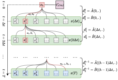
(a) Entire game tree

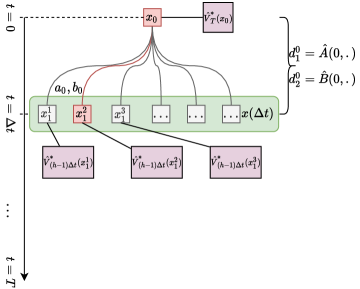
(b) Reduced game tree

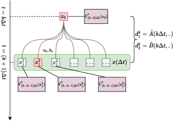
(c) Recursive form

Figure 1: (a) To compute $\hat{V}^{*}_{T}(x_{0})$, we need to traverse the entire game tree, then $\hat{V}^{*}_{T}(x_{0})=\mathscr{N}_{d_{1}^{0},...,d_{1}^{h-1},d_{2}^{0},...,d_{2}^{h-1}}\mathbb{E}\big{\{}[l(x_{0},a_{0},b_{0})+l(x(\Delta t),a_{1},b_{1})+...$ $+l(x((h-1)\Delta t),a_{h-1},b_{h-1})]\Delta t\big{|}a_{0}\sim d_{1}^{0},...,a_{h-1}\sim d_{1}^{h-1},b_{0}\sim d_{2}^{0},...,b_{h-1}\sim d_{2}^{h-1}\big{\}}$. (b) Given the state-value function $\hat{V}^{*}_{(h-1)\Delta t}(.)$, $\hat{V}^{*}_{T}(x_{0})=\mathscr{N}_{d_{1}^{0},d_{2}^{0}}\mathbb{E}[l(x_{0},a_{0},b_{0})\Delta t+\hat{V}^{*}_{(h-1)\Delta t}(x(\Delta t))|a_{0}\sim d_{1}^{0},b_{0}\sim d_{2}^{0}]$. (c) For any $k\in\{1,...,h\}$, we can obtain $\hat{V}^{*}_{(h-k)\Delta t}(.)$ via recursion: $\hat{V}^{*}_{(h-k)\Delta t}(x_{0})=\mathscr{N}_{d_{1}^{k},d_{2}^{k}}\mathbb{E}[l(x_{0},a_{k},b_{k})\Delta t+\hat{V}^{*}_{(h-k-1)\Delta t}(x(\Delta t))|a_{k}\sim d_{1}^{k},b_{k}\sim d_{2}^{k}]$.

According to Equation (13), for any $m=1,2,...$, $\hat{V}_{m\Delta t}^{*}(.)$ can be obtained by $m$-step recursion. There are infinite elements in set $\mathcal{A}$ and $\mathcal{B}$, thus, both players have infinite actions to be taken. However, traversing the entire $\mathcal{A}$ and $\mathcal{B}$ is impossible. Fortunately, many of those actions are very similar, we can just consider two sets of finite elements that distribute evenly in $\mathcal{A}$ and $\mathcal{B}$ instead of the entire ones. This is referred to as action abstraction [29] [30]. We represent the action abstractions of $\mathcal{A}$ and $\mathcal{B}$ as $\bar{\mathcal{A}}$ and $\bar{\mathcal{B}}$ respectively and denote the $i$th element in $\bar{\mathcal{A}}$ and $\bar{\mathcal{B}}$ as $\bar{\mathcal{A}}[i]$ and $\bar{\mathcal{B}}[i]$ respectively.

Given the state-value function $\hat{V}_{(k-1)\Delta t}^{*}(.)$ and the the action abstractions $\bar{\mathcal{A}}$ and $\bar{\mathcal{B}}$, the second equation in (13) can be translated into a normal-form game: Construct a $N_{a}\times N_{b}$ game matrix $\hat{\mathcal{G}}_{k}$ ($N_{a}$ and $N_{b}$ are the numbers of elements in $\bar{\mathcal{A}}$ and $\bar{\mathcal{B}}$), where each dimension has rows/columns corresponding to a single player’s actions [31]. By convention, the row player is player I and the column player is player II, and fill the entry in row $i$ column $j$ with

$$\hat{\mathcal{G}}_{k}[i][j]=l\left(x_{0},\bar{\mathcal{A}}[i],\bar{\mathcal{B}}[j]\right)\Delta t+\hat{V}_{(k-1)\Delta t}^{*}\left(F(x_{0},\bar{\mathcal{A}}[i],\bar{\mathcal{B}}[j])\right)$$ (13)

A part of the game matrix $\hat{\mathcal{G}}_{k}$ is shown in Fig. 2.

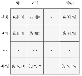
Figure 2: The game matrix $\hat{\mathcal{G}}_{k}$.

Then the regret matching can be adopted to compute the Nash equilibrium strategies, $d_{1}^{\hat{\mathcal{G}}_{k}*}\in\mathscr{D}_{\bar{\mathcal{A}}}$ and $d_{2}^{\hat{\mathcal{G}}_{k}*}\in\mathscr{D}_{\bar{\mathcal{B}}}$, for both players. Then, to compute $\hat{V}_{k\Delta t}^{*}(x_{0})$, sum over each action pair, the product of each player’s probability of playing their action in the action pair, times the value in the corresponding entry:

$$\hat{V}_{k\Delta t}^{*}(x_{0})=\sum_{i=1}^{N_{a}}\sum_{j=1}^{N_{b}}d_{1}^{\hat{\mathcal{G}}_{k}*}(\bar{\mathcal{A}}[i])d_{2}^{\hat{\mathcal{G}}_{k}*}(\bar{\mathcal{B}}[j])\hat{\mathcal{G}}_{k}[i][j]$$ (14)

Squently, making a little change on Algorithm 1, we can obtain an approximation of the Nash equilibrium state-value function $\hat{V}_{m\Delta t}^{*}(.)$ for $m=1,2,...$, see Algorithm 2 (with input $m=h$, we can obtain $\hat{V}_{T}^{*}(.)$).

Algorithm 2 Computation of Nash equilibrium state-value function

1:Input: Recursion number $m$;

2:Select a proper rectangular computational domain $\Omega=[\alpha_{l},\alpha_{u}]\times[\beta_{l},\beta_{u}]$;

3:Discretize $\Omega$ into a $N_{\alpha}\times N_{\beta}$ Cartesian grid structure;

4:Let $\mathcal{V}$ and $\mathcal{V}^{\prime}$ be two $N_{\alpha}\times N_{\beta}$ arrays and initialize them to $\mathbf{0}$;

5:for $k\leftarrow 1,...,m$ do

6:     for $i_{\alpha}\leftarrow 0,...,N_{\alpha}-1$ do

7:         for $i_{\beta}\leftarrow 0,...,N_{\beta}-1$ do

8:              $x\leftarrow\displaystyle{\left(\alpha_{l}+\frac{\alpha_{u}-\alpha_{l}}{N_{\alpha}-1}i_{\alpha}\beta_{l}+\frac{\beta_{u}-\beta_{l}}{N_{\beta}-1}i_{\beta}\right)^{\mathrm{T}}}$;

9:              Construct a $N_{a}\times N_{b}$ game matrix $\hat{\mathcal{G}}_{k}$;

10:              for $i\leftarrow 1,...,N_{a}$ do

11:                  for $j\leftarrow 1,...,N_{b}$ do

12:                       $a\leftarrow\bar{\mathcal{A}}[i]$;

13:                       $b\leftarrow\bar{\mathcal{B}}[j]$;

14:                       $x^{\prime}=F(x,a,b)$;

15:                       $\hat{\mathcal{G}}_{k}[i][j]\leftarrow l\left(x,a,b\right)\Delta t+\widehat{V}\left(x^{\prime}\right)$;

16:                  end for

17:              end for

18:              Use regret matching to compute $d_{1}^{\hat{\mathcal{G}}_{k}*}(.)$ and $d_{2}^{\hat{\mathcal{G}}_{k}*}(.)$;

19:              

$$\mathcal{V}^{\prime}[i_{\alpha}][i_{\beta}]\leftarrow\displaystyle{\sum_{i=1}^{N_{a}}\sum_{j=1}^{N_{b}}d_{1}^{\hat{\mathcal{G}}_{k}*}(\bar{\mathcal{A}}[i])d_{2}^{\hat{\mathcal{G}}_{k}*}(\bar{\mathcal{B}}[j])\hat{\mathcal{G}}_{k}[i][j]};$$

20:         end for

21:     end for

22:     Copy $\mathcal{V}^{\prime}$ to $\mathcal{V}$;

23:end for

24:Return $\widehat{V}(.)$;

3.3 Control policy

At time $t$, the actual optimal control inputs should be sampled from the initial distributions of $\hat{A}^{*}(.,.)$ and $\hat{B}^{*}(.,.)$, that is

$$\begin{split}a(t)\sim\hat{A}^{*}(0,.),b(t)\sim\hat{B}^{*}(0,.)\end{split}$$ (15)

where

$$\begin{split}(\hat{A}^{*}(.,.),\hat{B}^{*}(.,.))=\arg\mathop{\mathscr{N}}_{\hat{A},\hat{B}}\hat{V}_{T}(x(t),\hat{A}(.,.),\hat{B}(.,.))\end{split}$$ (16)

According to Equation (13), with a small enough $\Delta t$,

$$(\hat{A}^{*}(0,.),\hat{B}^{*}(0,.))=\arg\mathop{\mathscr{N}}_{d_{1}\in\mathscr{D}_{\mathcal{A}},d_{2}\in\mathscr{D}_{\mathcal{B}}}\mathbb{E}\bigg{[}l\left(x(t),a,b\right)\Delta t+\hat{V}_{(h-1)\Delta t}^{*}\left(F(x(t),a,b)\right)\bigg{|}a\sim d_{1},b\sim d_{2}\bigg{]}$$ (17)

holds. Therefore, given the state-value function $\hat{V}^{*}_{m\Delta t}(.)$ generated by Algorithm 2 with $m=h-1$, $\hat{A}^{*}(0,.)=d_{1}^{\mathcal{G}*}$ and $\hat{B}^{*}(0,.)=d_{2}^{\mathcal{G}*}$, where $\mathcal{G}$ is a game matrix, and

$$\mathcal{G}[i][j]=l\left(x(t),\bar{\mathcal{A}}[i],\bar{\mathcal{B}}[j]\right)\Delta t+\hat{V}^{*}_{(h-1)\Delta t}\left(F(x(t),\bar{\mathcal{A}}[i],\bar{\mathcal{B}}[j])\right)$$ (18)

In the question of on-line control, the state-value function $\hat{V}_{(h-1)\Delta t}(.)$ can be held in memory. Then construct a game matrix $\mathcal{G}$ and fill it using Equation (19). Finally, the Nash equilibrium strategy pair $(d_{1}^{\mathcal{G}*},d_{2}^{\mathcal{G}*})$ can be obtained via regret matching. Under the Nash equilibrium, no player can increase its own expected payoff (the performance index in the moving time frame for player I and the minus of it for player II) by changing only their own strategy, therefore, each player just needs to choose its own action according to its onw Nash equilibrium strategy and does not need to focus on the action taken by its opponent. Take player I as an example, its control block diagram is shown in Fig. 3.

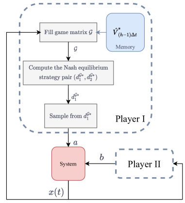
Figure 3: Control block diagram of player I.

4 Numerical Examples

The dynamics of the benchmark nonlinear plant can be expressed by

$$\dot{x}=\left[\begin{array}[]{c}\dot{\alpha}\\ \dot{\beta}\end{array}\right]=\left[\begin{array}[]{c}-(\alpha+\beta+a)^{3}\\ -(\beta-\alpha+b)^{3}\end{array}\right]=f(x,a,b)$$ (23)

where $a\in\mathcal{A}=[-1,1]$, $b\in\mathcal{B}=[-1,1]$.

4.1 Example 1

The running payoff function is expressed as:

$$l(x,a,b)=1+\alpha^{2}-\beta^{2}-a^{2}+b^{2}$$ (24)

The time step size is set as $\Delta t=0.02$. The computational domain is set as $\Omega=[-1,1]\times[-1,1]$. We discretize $\Omega$ into a $257\times 257$ Cartesian grid structure. And the action abstractions are

$$\bar{\mathcal{A}}=\bar{\mathcal{B}}=\left\{-1+0.05i|i=0,...,40\right\}$$ (25)

4.1.1 Computation of state-value functions

Given a $T$, the upper and lower state-value functions $V_{T}^{u}(.)$ and $V_{T}^{l}(.)$ can be approximated via Algorithm 1. And the Nash equilibrium state-value function $V_{T}^{*}(.)$ can be approximated via Algorithm 2. Fig. 4 shows $V_{T}^{u}(.)$, $V_{T}^{l}(.)$ and $V_{T}^{*}(.)$ under $T=1$ (in Algorithm 1 and Algorithm 2, input $m=50$). It can be seen that $V_{1}^{u}(.)=V_{1}^{l}(.)$, that means the saddle point exists. Therefore, as expected, $V_{1}^{u}(.)=V_{1}^{l}(.)=V_{1}^{*}(.)$. We show the optimal actual control inputs and game matrix at states $(0.5,0.5)^{\mathrm{T}}$ and $(0.3,0.8)^{\mathrm{T}}$ with $V_{1}^{*}(.)$ kept in memory, see Fig. 5. As expected, both players choose a single action with probability 1.

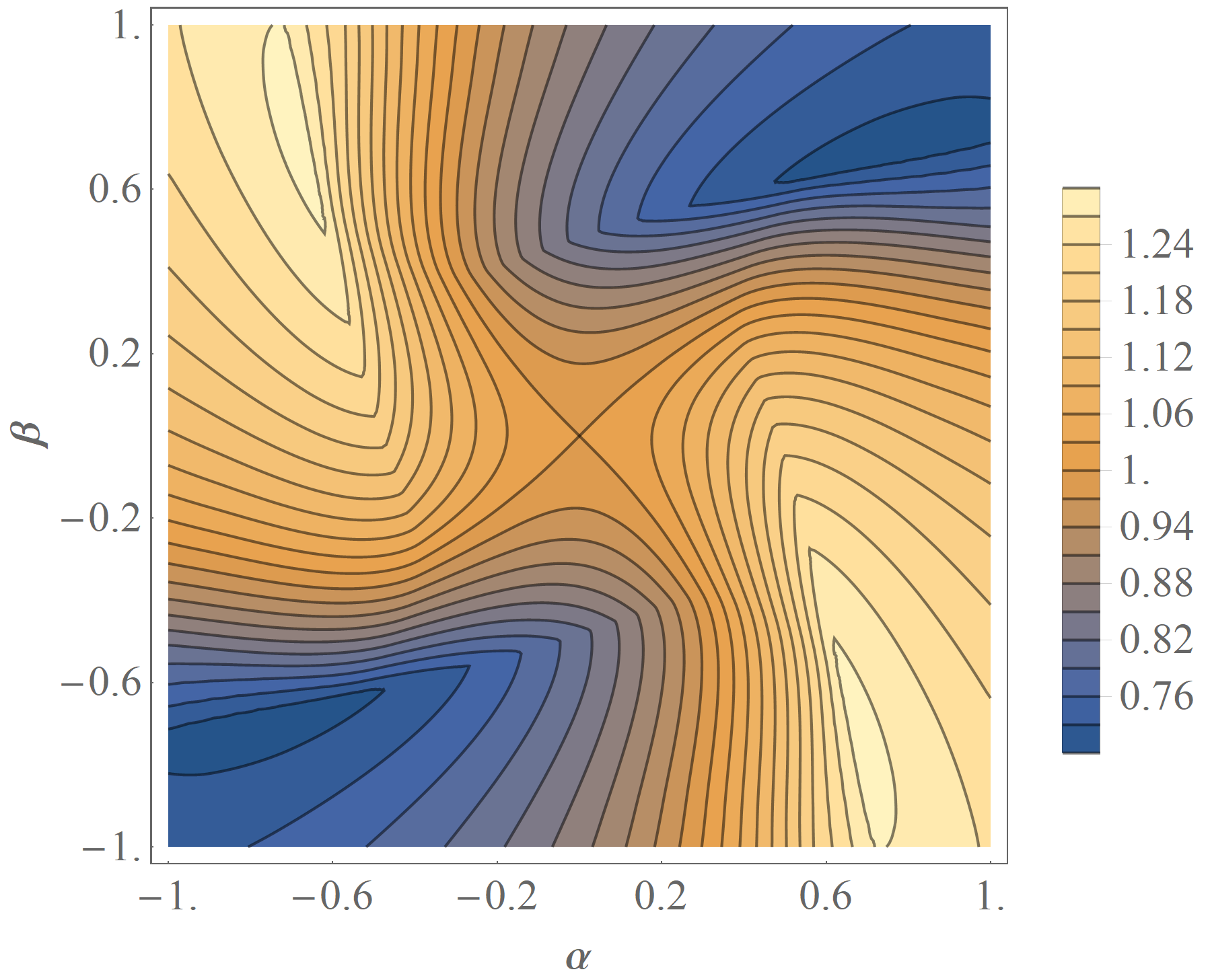
(a) $V^{u}_{1}(.)$

(b) $V^{l}_{1}(.)$

(c) $V^{*}_{1}(.)$

Figure 4: The upper, lower and Nash equilibrium state-value functions under $T=1$.

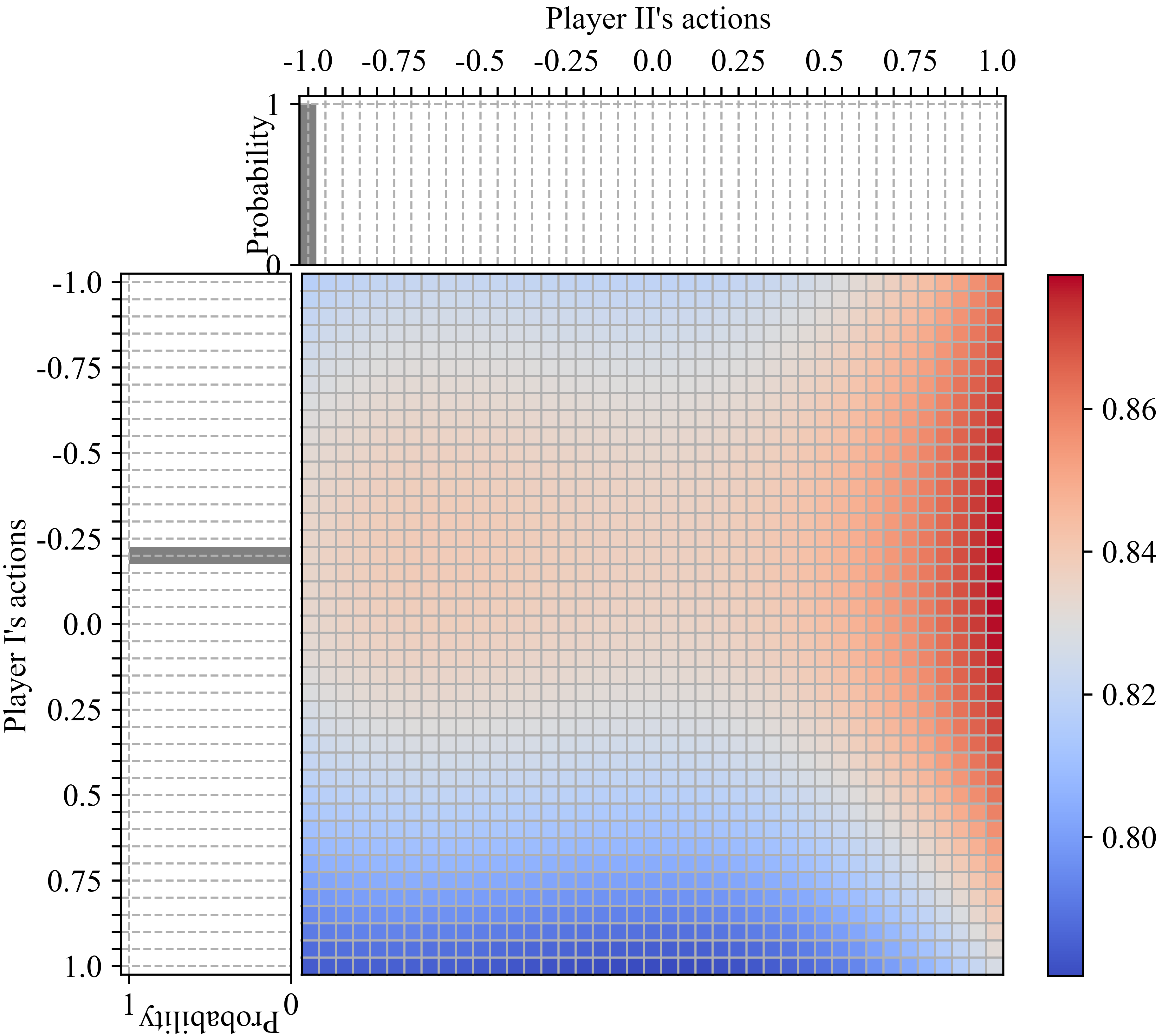
(a) Optimal actual control inputs and game matrix at state $(0.5,0.5)^{\mathrm{T}}$

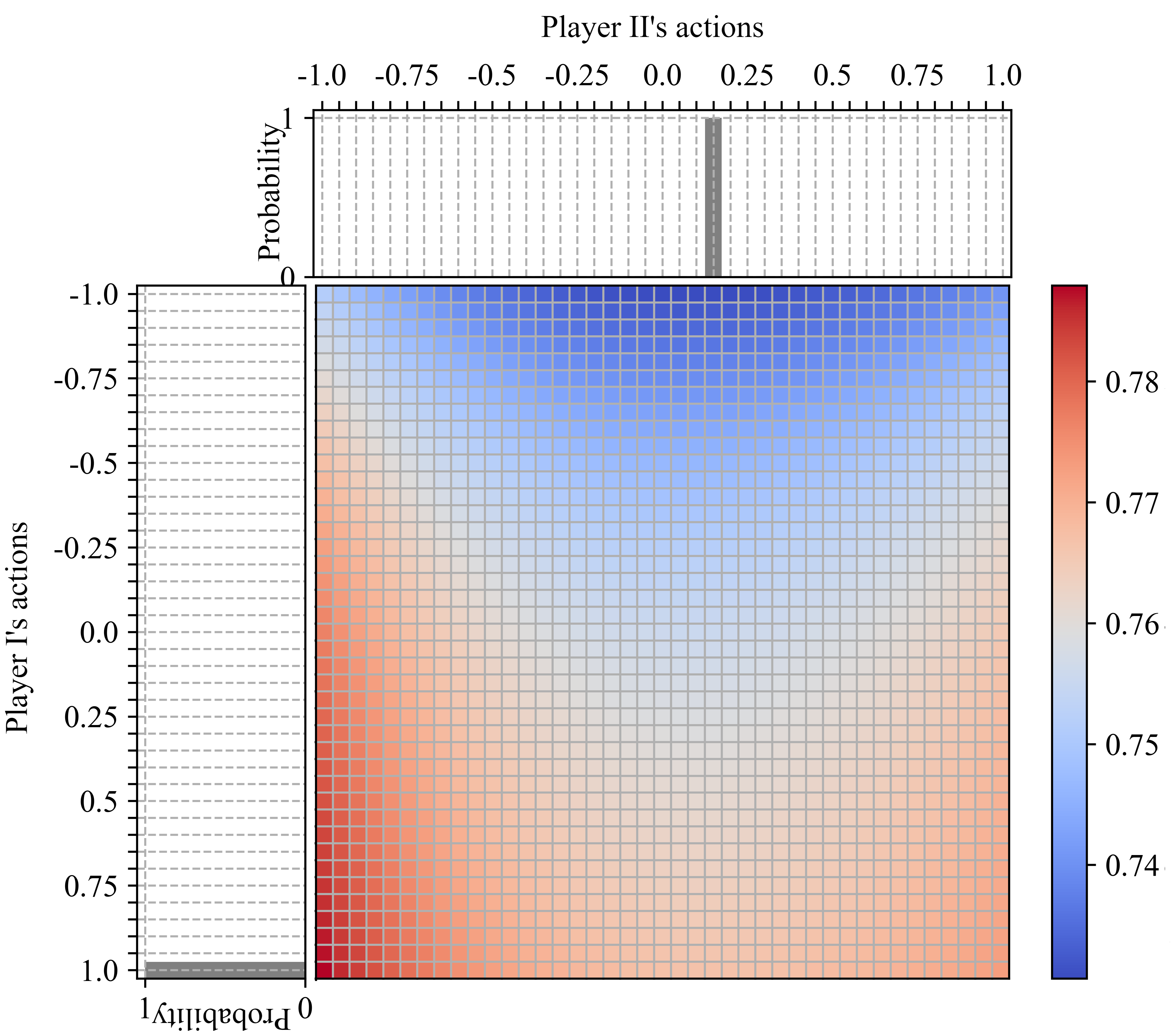
(b) Optimal actual control inputs and game matrix at state $(0.3,0.8)^{\mathrm{T}}$

Figure 5: (a) At state $(0.5,0.5)^{\mathrm{T}}$, player I chooses the single action $a=0.2$ with probability 1, player II chooses the single action $b=0$ with probability 1. (b) At state $(0.3,0.8)^{\mathrm{T}}$, player I chooses the single action $a=1$ with probability 1, player II chooses the single action $b=0.15$ with probability 1. The values in different entries of the game matrix are expressed as different colors.

4.1.2 Battle between different control policies

To demonstrate the effectiveness of our method, some battles between different control policies are simulated. These optional control policies include our method and the control policies with the existence hypothesis of saddle points. The later can be categorized into two types:

• The Min-max type: This type aims to find the optimal control input corresponding to the upper state-value function.

• The Max-min type: This type aims to find the optimal control input corresponding to the lower state-value function.

The rolling optimization with predictive period $T=1$ are adopted in all the control policies. When a player take our method, the state-value function $\hat{V}^{*}_{0.98}(.)$ computed by Algorithm 2 (input $m=49$) is kept in its memory. For each control policy pair, we take 100 simulations with random initial states and the average value of these simulations’ cumulative payoff is calculated. The duration of these simulations are set as 10. The process of a battle between two control policies is shown in Fig. 6.

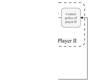
Figure 6: Block diagram of a battle.

The battle results are shown in Table 1. It can be seen that the values in different entries of Table 1 have no significant difference, this happened due to the existence of the saddle point, the control inputs generated by these three control policies are same.

Table 1: Battle results of Example 1.

		Player II’s control policy
		Min-max type	Max-min type	Our method
Player I’s control policy	Min-max type	10.03673	10.03351	10.03608
	Max-min type	10.0347	10.0284	10.0306
	Our method	10.0293	10.0325	10.0289

4.2 Example 2

In this example, the running payoff function is changed as

$$l(x,a,b)=1+10\sin(4ab)+\alpha^{2}-\beta^{2}$$ (26)

All other settings are the same as the ones in Example 1.

4.2.1 Computation of state-value functions

The upper and lower state-value functions under predictive period $T=1$s are shown in Fig. 7(a) and (b). It can be seen that $V_{1}^{u}(.)\neq V_{1}^{l}(.)$, that means the saddle point does not exist, we can only use Algorithm 2 to compute the Nash equilibrium state-value function, see Fig. 7(c). In order to visually display the mixed optimal actual control inputs, we show the optimal actual control inputs and game matrix at states $(0.2,-0.2)^{\mathrm{T}}$ and $(0.3,0.35)^{\mathrm{T}}$ with $V_{1}^{*}(.)$ kept in memory, see Fig. 8. Since the saddle point dose not exist, both players have many actions that are played with positive probability.

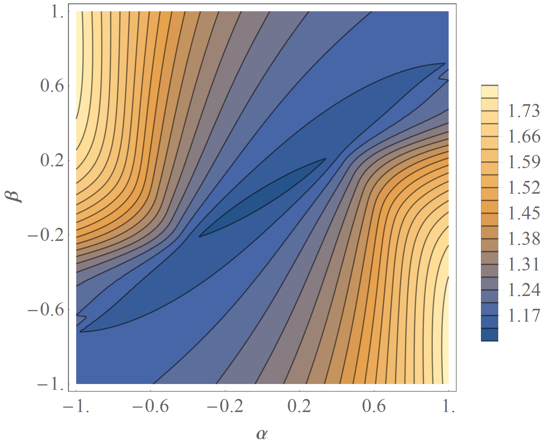
(a) $V^{u}_{1}(.)$

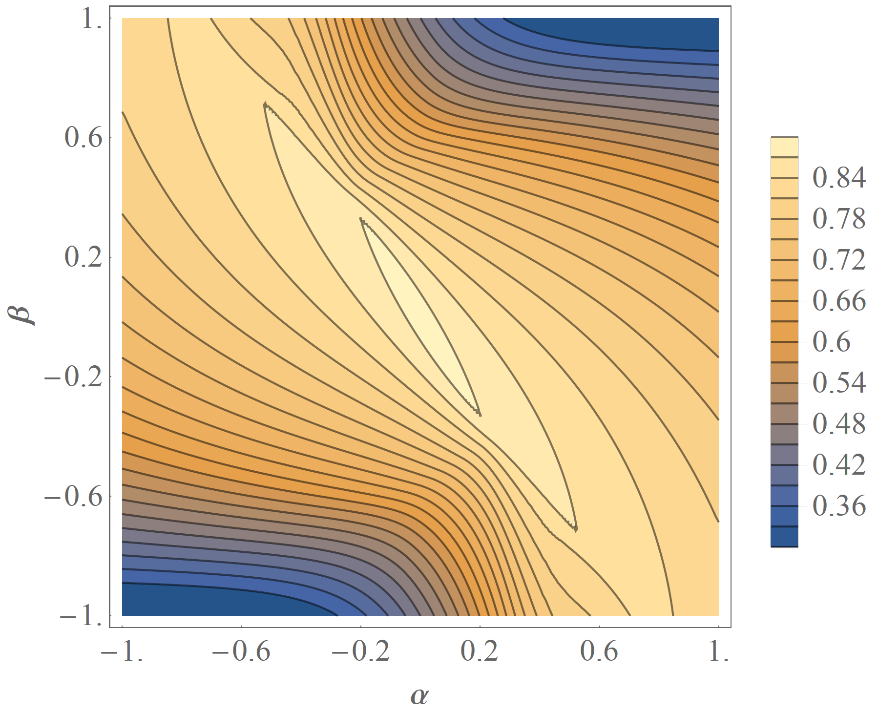
(b) $V^{l}_{1}(.)$

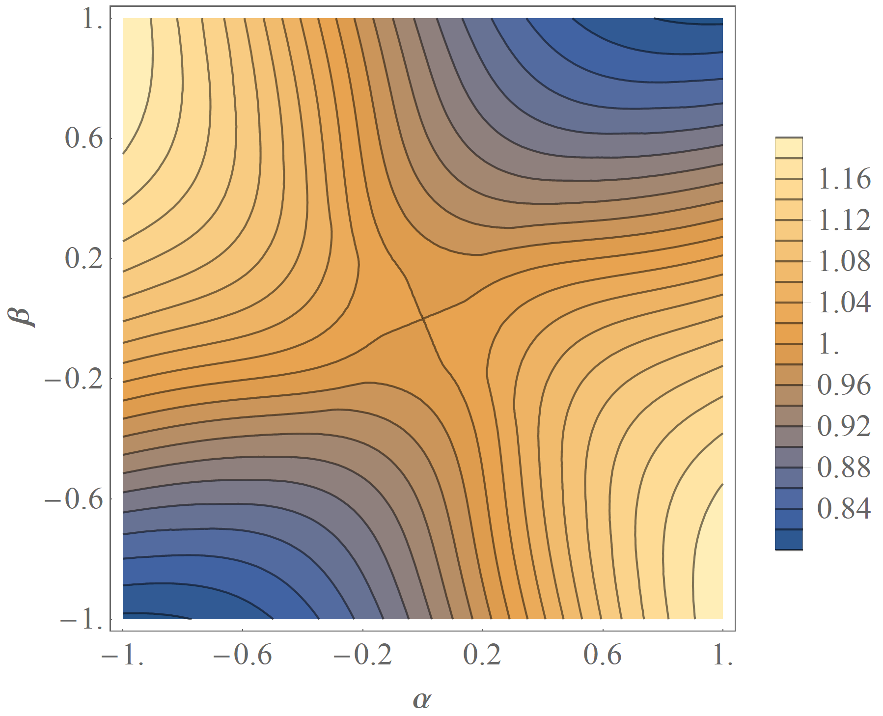
(c) $V^{*}_{1}(.)$

Figure 7: The upper, lower and Nash equilibrium state-value functions under $T=1$.

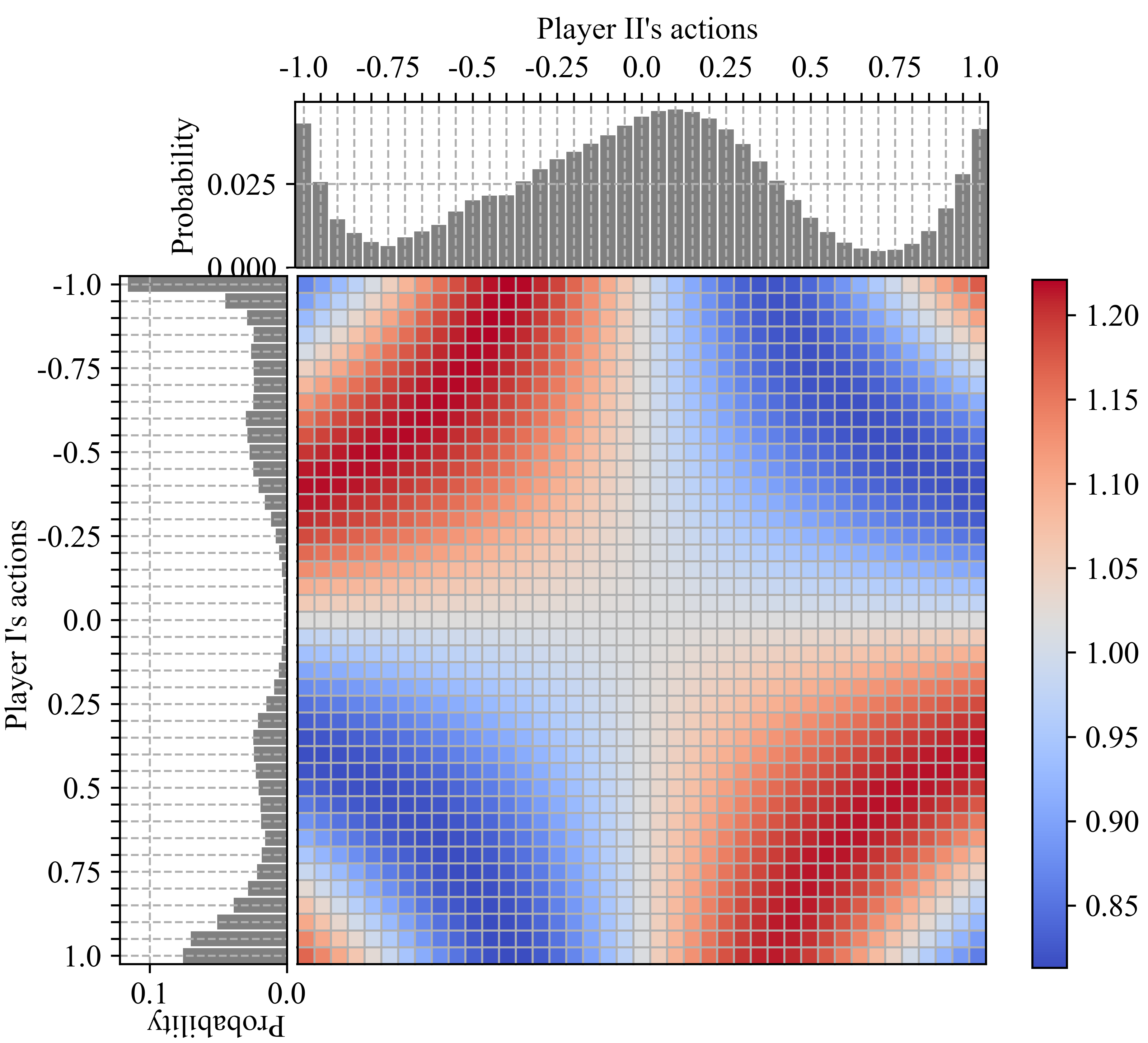
(a) Optimal actual control inputs and game matrix at state $(0.2,-0.2)^{\mathrm{T}}$

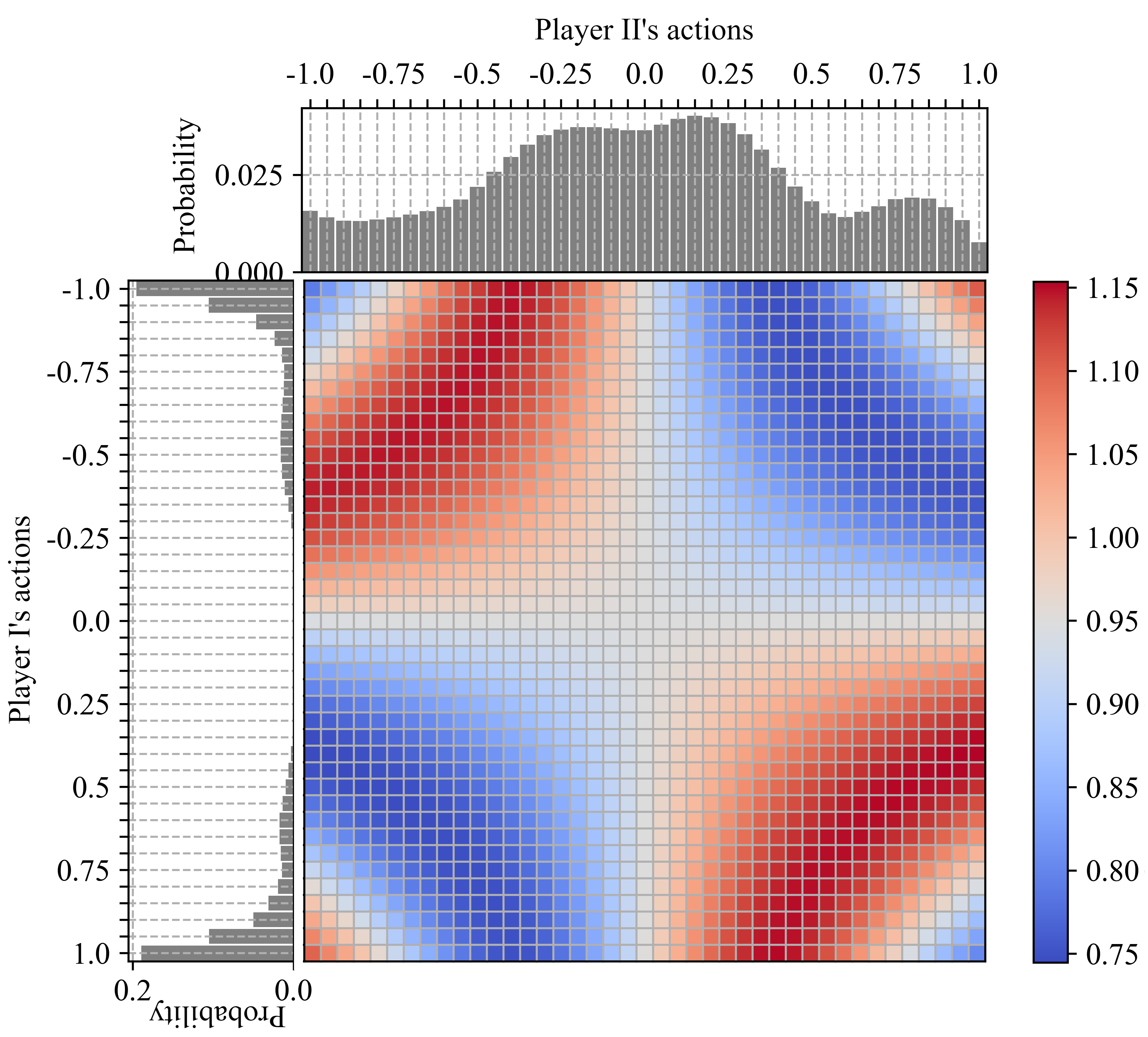
(b) Optimal actual control inputs and game matrix at state $(0.3,0.35)^{\mathrm{T}}$

Figure 8: At state $(0.2,-0.2)^{\mathrm{T}}$ and $(0.3,0.35)^{\mathrm{T}}$, both players have many actions that are played with positive probability. The values in different entries of the game matrix are expressed as different colors.

4.2.2 Battle between different strategies

In this example, we also simulate some battles between different control policies. The settings are the same as the ones in Example 1. The simulation results are shown in Table 2. Table 2 shows that, the values in different entries have significant difference. For player II, compared to other control policies, our method is a dominant control policy. That is, for player II, choosing our method always gives a better outcome than choosing other control policies, no matter what player I do. For player I, the best control policy is our method when player II chooses our method as its control policy.

Table 2: Battle results of Example 2.

		Player II’s control policy
		Min-max type	Max-min type	Our method
Player I’s control policy	Min-max type	16.7026	15.23	7.5577
	Max-min type	10.4195	11.5609	8.1819
	Our method	11.6277	11.7377	8.5097

5 Conclosions

In this paper, a method is developed to solve the rolling Nash equilibrium of zero-sum differential games. The first step is discretize time into several intervals with small size. Then, with the aid of state-value function, the differential game is translated into a recursion consisting of normal-form game, and based on the action abstraction and regret matching the Nash equilibrium of each normal-form game can be obtained. When use our method to deal with a on-line control problem, the state-value function can be stored in memory to improve the real-time property. This method is effective for both the situations that the saddle point exists or does not exist. The analysis of existence of the saddle point are avoided. For the situation that the saddle point exists, our method can give the pure control policy. For the situation that the saddle point does not exist, our method can give the probability distribution of the mixed control policy. In order to improve the accuracy and reduce the grid quantity, possible future developments will address a more advanced interpolation method instead of the linear interpolation described here.

Appendix

In this section, we introduce the linear interpolation applied in this paper. Let $x_{0}$ denote a system state, and $x_{1}$, $x_{2}$, $x_{3}$ are the three nearest grid points around $x_{0}$. These three grid points can constitute a right triangle cell. The coordinate of $x_{i}$ is denoted as $(\alpha_{i},\beta_{i})$. According to the nearest grid point of $x_{0}$, the interpolation can be divided into four cases, see Fig. 9. Let $V_{i}$ denote the state-value of point $x_{i}$ (the state-value of the grid points are stored in the two-dimensional array $\mathcal{V}$). The goal of interpolation is to estimate $V_{0}$.

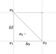
(a) The nearest grid point is located at the bottom left.

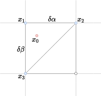
(b) The nearest grid point is located at the top left.

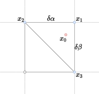
(c) The nearest grid point is located at the top right.

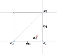
(d) The nearest grid point is located at the bottom right.

Figure 9: Interpolation of different cases.

The explanations of the symbols in Fig. 9 are as following:

$$\delta\alpha=\alpha_{2}-\alpha_{1},\delta\beta=\beta_{3}-\beta_{1}$$ (27)

Then

$$V_{0}=\frac{V_{2}-V_{1}}{\delta\alpha}(\alpha_{0}-\alpha_{1})+\frac{V_{3}-V_{1}}{\delta\beta}(\beta_{0}-\beta_{1})+V_{1}$$ (28)

References

- [1] Min-Jea Tahk, Hyeok Ryu, and Je-Gyum Kim. An iterative numerical method for a class of quantitative pursuit-evasion games.
- [2] Kyriakos Vamvoudakis and Frank Lewis. Multi-player non-zero-sum games: Online adaptive learning solution of coupled hamilton-jacobi equations. Automatica, 47:1556–1569, 08 2011.
- [3] Adriano Festa, R. Guglielmi, Cristopher Hermosilla, Athena Picarelli, Smita Sahu, Achille Sassi, and Francisco Silva. Hamilton-jacobi-bellman equations. Lecture Notes in Mathematics, 2180:127–261, 09 2017.
- [4] K. G. Vamvoudakis and F. L. Lewis. Online solution of nonlinear two-player zero-sum games using synchronous policy iteration. In 49th IEEE Conference on Decision and Control (CDC), pages 3040–3047, 2010.
- [5] D. Liu and Q. Wei. Finite-approximation-error-based optimal control approach for discrete-time nonlinear systems. IEEE Transactions on Cybernetics, 43(2):779–789, 2013.
- [6] Zhen Ni and Shuva Paul. A multistage game in smart grid security: A reinforcement learning solution. IEEE Transactions on Neural Networks and Learning Systems, PP:1–12, 01 2019.
- [7] M. I. Abouheaf, M. S. Mahmoud, and F. L. Lewis. Policy iteration solution for differential games with constrained control policies. In 2019 American Control Conference (ACC), pages 4301–4306, 2019.
- [8] Kyriakos Vamvoudakis and F.L. Lewis. Online solution of nonlinear two-player zero-sum games using synchronous policy iteration. volume 22, pages 3040–3047, 12 2010.
- [9] H. S. Chang, J. Hu, M. C. Fu, and S. I. Marcus. Adaptive adversarial multi-armed bandit approach to two-person zero-sum markov games. IEEE Transactions on Automatic Control, 55(2):463–468, 2010.
- [10] R. Jain and J. Watrous. Parallel approximation of non-interactive zero-sum quantum games. In 2009 24th Annual IEEE Conference on Computational Complexity, pages 243–253, 2009.
- [11] X. Zhong, H. He, D. Wang, and Z. Ni. Model-free adaptive control for unknown nonlinear zero-sum differential game. IEEE Transactions on Cybernetics, 48(5):1633–1646, 2018.
- [12] R. Song, J. Li, and F. L. Lewis. Robust optimal control for disturbed nonlinear zero-sum differential games based on single nn and least squares. IEEE Transactions on Systems, Man, and Cybernetics: Systems, pages 1–11, 2019.
- [13] J. Engwerda. Uniqueness conditions for the infinite-planning horizon open-loop linear quadratic differential game. In Proceedings of the 44th IEEE Conference on Decision and Control, pages 3507–3512, 2005.
- [14] Askar Rakhmanov, Gafurjan Ibragimov, and Massimiliano Ferrara. Linear pursuit differential game under phase constraint on the state of evader. Discrete Dynamics in Nature and Society, 2016:1–6, 01 2016.
- [15] M. Levy, T. Shima, and S. Gutman. Full-state autopilot-guidance design under a linear quadratic differential game formulation. Control Engineering Practice, 75(jun.):98–107, 2018.
- [16] Huaguang Zhang, Qinglai Wei, and Derong Liu. An iterative adaptive dynamic programming method for solving a class of nonlinear zero-sum differential games. Automatica, 47(1):207 – 214, 2011.
- [17] Martin Schmid, Neil Burch, Marc Lanctot, Matej Moravcik, Rudolf Kadlec, and Michael Bowling. Variance reduction in monte carlo counterfactual regret minimization (vr-mccfr) for extensive form games using baselines, 09 2018.
- [18] Sergiu Hart and Andreu Mas-Colell. A simple adaptive procedure leading to correlated equilibrium1. Econometrica, pages 1127–1150, 07 2000.
- [19] Todd W. Neller and Marc Lanctot. An introduction to counterfactual regret minimization, 2013.
- [20] Qi Tian and Jinhua Zhao. Regret minimization in decision making: Implications for choice modeling and policy design. 2018 Annual Meeting, August 5-7, Washington, D.C. 274016, Agricultural and Applied Economics Association, 2018.
- [21] V. Hakami and M. Dehghan. Learning stationary correlated equilibria in constrained general-sum stochastic games. IEEE Transactions on Cybernetics, 46(7):1640–1654, 2016.
- [22] Wen-Hua Chen, Donald Ballance, and Peter Gawthrop. Optimal control of nonlinear systems: A predictive control approach. Automatica, 39:633–641, 04 2003.
- [23] L. D. Berkovitz. Differential games of generalized pursuit and evasion. In 1985 24th IEEE Conference on Decision and Control, pages 1104–1105, 1985.
- [24] Tamer Basar and P. Bernhard. -optimal control and related minimax design problems : a dynamic game approach. Automatic Control IEEE Transactions on, 41(9):1397, 1991.
- [25] Tor Lattimore and Csaba Szepesvári. Markov Decision Processes, pages 452–483. 07 2020.
- [26] Marco Wiering and Martijn Otterlo. Reinforcement Learning: State-Of-The-Art, volume 12. 01 2012.
- [27] R. Myerson. Refinements of the nash equilibrium concept. Int J Game Theory, 7:73–80, 01 1978.
- [28] Luis von Ahn. Preliminaries of game theory. https://web.archive.org/web/20111018035629/http://scienceoftheweb.org/15-396/lectures_f11/lecture09.pdf.
- [29] Noam Brown and Tuomas Sandholm. Superhuman ai for heads-up no-limit poker: Libratus beats top professionals. Science, 359:eaao1733, 12 2017.
- [30] Noam Brown and Tuomas Sandholm. Safe and nested subgame solving for imperfect-information games. In Proceedings of the 31th International Conference on Neural Information Processing Systems, pages 689–699, 2017.
- [31] Eric Damme. A relation between perfect equilibria in extensive form games and proper equilibria in normal form games. International Journal of Game Theory, 13:1–13, 03 1984.