Anti-parallel links as boundaries of knotted ribbons
Abstract.
We consider a two component link which is the boundary of a knotted ribbon with knot type . If the two components of are assigned opposite (anti-parallel) orientations and is a special alternating knot, namely a knot with a reduced alternating knot diagram in which the crossings are all positive or all negative, we show that the braid index of is bounded below by , where is the minimum crossing number of . A long standing open conjecture states that the ropelength of any alternating knot is bounded below by its minimum crossing number multiplied by a positive constant. Using the above result, we are able to prove that this conjecture holds for the special alternating knots.
Key words and phrases:
knots, links, knotted ribbons, alternating knots and links, braid index, ropelength.2020 Mathematics Subject Classification:
Primary: 57K10, 57K31, 57K991. Introduction
A knotted ribbon with a given knot type is an embedding of the annulus into such that the centerline (axis) of the annulus is a knot of the given knot type . The boundary of a knotted ribbon with knot type is a two component link denoted by either or , depending on whether the two components are assigned parallel or anti-parallel orientations respectively. In [18] J. White proved the famous formula
| (1.1) |
where is the linking number of (a link invariant), is the twist of and is the writhe of the centerline (or the axis) of . Equation (1.1) has a very important application in DNA research since a knotted ribbon provided an ideal mathematics model for circular double stranded DNA in which the two sugar-phosphate backbones of the double helix are modeled by the boundary curves of the knotted ribbon [1]. Inspired by this work, in this paper we study another link invariant related to a link that is the boundary of a knotted ribbon, namely the braid index. The braid index of can be easily shown to be where is the braid index of , thus the case of interest to us is the braid index of .
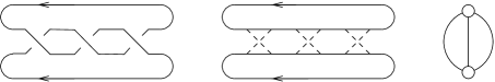
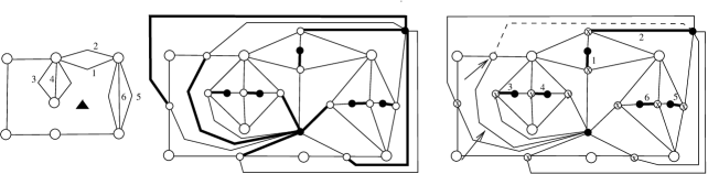
The main result of this paper is that if is an alternating knot with a reduced knot projection in which the crossings are either all positive or all negative (such an alternating knot is called a special alternating knot by Murasugi in [15]), then the braid index of is bounded below both by the minimum crossing number of and the absolute linking number of (multiplied by some positive constant). More specifically, let be an alternating knot with a reduced knot projection in which the crossings are either all positive or all negative, then admits a projection diagram as depicted in Figure 1, where the two components of are realized as and a parallel copy of (but with opposite orientations). A crossing in becomes a 4 crossing junction in . The additional full twists between these two components are determined by , where is the writhe of the diagram (namely the sum of the number of positive crossings minus the number of negative crossings in ). and indicate that the crossings in these full twists are positive or negative respectively. Let be the number crossings in and be the number of Seifert circles (to be discussed in the next section), then our main result can be formulated as the following theorem.

Theorem 1.1.
Let be a special alternating knot with a reduced alternating link diagram such that , then the braid index of , which is the same as that of with , is bounded below by where
Since grows linearly in terms of (after it passes some threshold), the braid index of is bounded below by plus a linear term of . This result has a significant implication concerning the ropelength problem of knots as explained below.
The ropelength of a link is defined (intuitively) as the minimum length of unit thickness ropes needed to tie the link. Let be an un-oriented link, be the minimum crossing number of and be the ropelength of . A fundamental question in geometric knot theory asks how is related to . In general the determination of the precise ropelength of a non-trivial link is a difficult problem and no known precise formula exists for even for the simplest nontrivial knot, namely the trefoil. However we have gained much knowledge about the asymptotic behavior of in terms of . For example, it is known that for some positive constants and for any [2, 3, 8], and for any power that is between and , there exist families of infinitely many links such that the ropelength of links from these families grows proportionally to [4, 5, 6, 9]. It has been conjectured that the ropelength of any alternating link is at least proportional to its crossing number. While this conjecture has been shown to be true for alternating links whose maximum braid indices are proportional to their crossing numbers, it is still wide open in general. Using the main result of this paper, we are able to prove that this conjecture holds for all special alternating knots regardless whether their braid indices are proportional to their crossing numbers.
We arrange the rest of the paper as follows. In the next section, we introduce the Seifert circle decomposition of oriented link diagrams and their corresponding Seifert graphs. Some graph theory terminology specific to this paper will also be introduced. In Section 3 we introduce the Murasugi-Przytycki reduction operation. Some important results regarding the HOMFLY-PT polynomial are given in Section 4 as the HOMFLY-PT polynomial is our main tool in estimating the braid index. Section 5 is devoted to the proof of Theorem 1.1 and contains the bulk of the technical details of this paper. In the last section we apply 1.1 to the ropelength problem of knots.
2. Seifert circle decomposition and Seifert graphs
2.1. Seifert circle decomposition
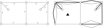
The Seifert circle decomposition of is the collection of disjoint topological circles (called Seifert circles or -circles for short) obtained after all crossings in are smoothed (as shown in Figure 2). Notice that since is positive and is alternating, it can be drawn in a way that no -circle can contain other -circles in its interior.
2.2. Trapped -circles
Consider three -circles , and as shown in Figure 3 where is bounded within the topological disk created by arcs of , and the two consecutive crossings as shown in the figure. We say that is trapped between and . Similarly, is also trapped between and . Since is a special knot diagram in our case, the interior of any -circle does not contain any other -circle. Thus we can always use flype moves to free any trapped -circles, hence we can assume that is free of trapped -circles from this point on. An immediate consequence of this is that if two -circles and share crossings, then as we travel along either or , we encounter all these crossings consecutively without running into crossings between them and other -circles.

2.3. Seifert graphs
We assume that our reader has the basic knowledge of graph theory and will only define the concepts that are specific to this paper. The common graph theory terminology used in this paper can be found in standard textbooks such as [17].
Definition 2.1.
Let be a reduced alternating diagram, then shrinking each -circle to a vertex and changing each crossing between two -circles to an edge connecting the two corresponding vertices, we obtain a (bipartite) plane graph. We denote this graph by and call it the Seifert graph of . See the right side of Figure 2 for an example.
If two -circles in share one and only one crossing between them, then this crossing is called a lone crossing. Two -circles in sharing a lone crossing corresponds to two vertices in connected by one and only one edge which we shall call a lone edge. Notice that a lone edge in cannot be a bridge, since otherwise it would correspond to a nugatory crossing of , but that is not possible since is reduced. Sometimes it is more convenient to use a different version of the Seifert graph of , denoted by . is similar to except that it is a simple graph with its edges weighted. An edge of weight in connecting two vertices and corresponds to the case when the same vertices and in are connected by edges. A lone edge in is an edge of weight one in . Since is a knot, cannot contain a bridge edge of even weight.
Definition 2.2.
A face of a plane graph is said to be non-separating if deleting the edges on its boundary does not disconnect the graph . The graph is said to be proper if every face of it is non-separating. is said to be proper if every face in is non-separating. See Figure 4 for an example.
Definition 2.3.
A set of edges in is said to be a maximal 2-cut set if it satisfies the following conditions: (i) contains only lone edges and ; (ii) deleting any two edges in disconnects and (iii) no other lone edges can be added to in order for (ii) to hold.
Remark 2.4.
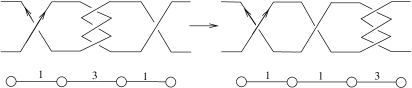
If contains a maximal 2-cut set , then we can perform flypes on so that in the resulting knot diagram , the lone crossings corresponding to the lone edges in occur in a consecutive manner. In other word, if is the new diagram, then the lone edges in form a path in such that the internal vertices of this path are all of degree 2. Thus from this point on we will assume that a maximal 2-cut set of , if it exists, consists of a path of lone edges whose internal vertices are all of degree 2. See Figure 5 for an illustration of a simple case.
Lemma 2.5.
Let be a special alternating knot diagram, then the following conditions are equivalent.
(i) is proper;
(ii) For any face of , there exists a spanning tree of such that no edges on are on the boundary of .
(iii) does not contain any maximal 2-cut set.
Proof.
(i) (ii) If is proper and is any face of , then deleting the edges on the boundary of does not disconnect the graph, which means we can construct a spanning tree of without using any edges on . (ii) (iii) If contains a maximal 2-cut set , then it is necessary that the lone edges in are all on the boundary of a face . Since deleting any two lone edges in will disconnect , this means that if we delete the edges on the boundary of , we will disconnect as well. Thus it is not possible for us to construct a spanning tree of without using edges on the boundary of , which contradicts the given condition. (iii) (i) Consider any face of . First consider the case that contains a cycle in which has length 2 and corresponds to an edge of weight at least 2 in . If is not a bridge edge of , then deleting the edges in obviously will not disconnect . If is a bridge edge of , then it is necessary that its weight is an odd integer that is at least 3 since is a reduced knot diagram. Therefore deleting the edges in will not disconnect either. If contains a cycle that is of length at least 4, then let us remove the edges of one at a time. If the edge removed is not a lone edge, then obviously this does not disconnect . If the edge is the first lone edge encountered, removing the edge will not disconnect either since the lone edge cannot be a bridge edge. Thus the only way becomes disconnected is when we encounter a second lone edge in . But this means that a maximal 2-cut set exists which contradicts the given condition. Since the boundary of consists of cycles, this proves that removing the boundary of will not disconnect . ∎
For any plane graph , its number of faces is given by , where and are the number of edges and vertices of respectively. In the case that , we have and , where and are the number of crossings and number of -circles in respectively.
3. The Murasugi-Przytycki reduction operation
Consider a link diagram with the property that none of its Seifert circles contains other Seifert circles in its interior. Here is more general, not necessarily a positive or negative alternating knot diagram. If has a lone crossing between two -circles and , then we can reroute the overpass at this crossing as shown in Figure 6.


The overpass to be rerouted is marked by a thick line in the top left diagram of Figure 6 and the rerouted pass is marked by the thick line in the top right diagram (the thick line is the over strand at each crossing). The effect of this rerouted strand to the Seifert circle decomposition is that and are combined into one -circle , and any -circle sharing crossings with becomes an -circle contained within this new -circle (we say that is swallowed by ), while any -circle sharing crossings with will now share the same crossings with instead. If we ignore the -circles swallowed by , then the effect of this operation on is that the vertices , corresponding to , , and any vertex corresponding to an -circle sharing crossings with , is contracted to the same vertex . The bottom of Figure 6 shows this effect on the Seifert graph of the diagram. Notice that in the above described operation, we can also use in the place of , which will lead to a different diagram and a different Seifert graph as it will contract the vertices connected with instead. This operation is known as the Murasugi-Przytycki reduction operation (we shall call it the MP operation for short) [16].
Definition 3.1.
For a given link diagram , we use and to denote the maximum number of MP operations that can be performed on positive and negative lone crossings respectively.
Remark 3.2.
If a lone crossing is positive (negative), then applying the MP operation to the diagram results in a new diagram with and (), since the overpass crosses an existing Seifert circle an even number of times in the re-routing process hence does not change the writhe of except that the lone positive (negative) crossing is eliminated. Thus in general, can be deformed via the MP operations to new diagrams and such that , and , .
4. The HOMFLY-PT polynomial
Let us recall that the HOMFLY-PT polynomial of an oriented link is defined using any diagram of the link with the following rules: (a) If and represent the same link, then ; (b) if is an unknot and (c) where , and are identical link diagrams except at one crossing as shown in Figure 7. For the sake of simplicity we shall use for .

For our purposes, we will actually be using the following two equivalent forms of the skein relation (c) above:
| (4.1) | |||||
| (4.2) |
For any Laurent polynomial of variables and , we will use and to denote the highest and lowest power of in . Furthermore, if we write as a polynomial of with polynomials of as its coefficients, then the highest power term in the coefficient polynomials of the and the terms are denoted by and respectively (these are monomials in the variable ). In the case that , we will abbreviate , , and by , , and respectively.
Example 4.1.
For example, if is the positive torus link with its two components assigned anti-parallel orientations, we have . Hence , , and .
Given an oriented link diagram , let be the writhe of and be the number of Seifert circles in . The following result is well known.
Proposition 4.2.
Corollary 4.3.
Let be any link diagram, then and .
Proof.
By Remark 3.2, is equivalent to with and , thus we have . Similarly, . ∎
In the rest of this paper, we will use to denote the number of crossings in the diagram . If is a positive diagram (meaning the crossings in are all positive), then . The following result is known, it can be proved using the two special link trivialization operations called Operations P and N in [10]. Note that it is applicable to any link diagram whose crossings are all positive, the link diagrams do not have to be alternating.
Proposition 4.4.
Let be a positive link diagram (that is, all crossings in are positive), then and .
We shall also need the following two well known equalities regarding the HOMFLY-PT polynomial.
Proposition 4.5.
[12] Let and be two links and let , be the connected sum and disjoint sum of and respectively, then
and
5. The proof of the main result
We divide the proof of the theorem into several subsections to make it easier for our reader to follow. Furthermore, we will only consider the case when the is a positive diagram. If is a negative diagram, we can consider its mirror image instead since the braid index does not change when we pass from a link to its mirror image. Our goal is to derive explicit formulas for and , from which we can then calculate and apply Proposition 4.2.
5.1. The Seifert graph of
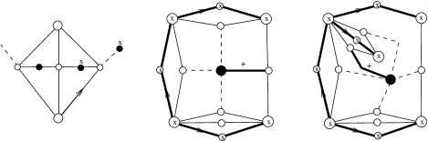
We shall take a systematic approach to obtain and to gain a good understanding of it. Let us choose a parallel copy of so that its strand is always on our right hand side as we travel on the strand of following its orientation. Figure 8 shows the details at a crossing of and the corresponding crossing junction in . The crossing is positive and must be between two distinct Seifert circles and as marked by dashed lines in the figure. Since and have different orientations, the two positive crossings are between strands from the same component while the negative crossings involve strands from different components. After smoothing the crossings, it is obvious that and remain -circles, with another -circle inserted between them and this new -circle shares a lone positive crossing both with and . Extending this to all other 4 crossing-junctions of , we see that in general all -circles with anti-clockwise orientation consist of strands of while all -circles with clockwise orientation consist of strands of . Furthermore, -circles of can be divided into three groups. The first group contains the original -circles from which we shall call large -circles. The second group contains the -circles created in the middle of each 4 crossing-junction of as shown in Figure 8. Each such -circle corresponds to a crossing of and shares lone crossings with two and only two large -circles. We shall call these -circles medium -circles). The third group contains the remaining -circles, which are obtained by deleting the negative crossings in and we shall call these small -circles. Let us call the vertices in corresponding to large, medium and small -circles large, medium and small vertices respectively. Notice that each medium -circle also shares lone negative crossings with exactly two small -circles.

Let us denote by the (positive) diagram that contains the large -circles and the medium -circles. and can be constructed from in the following way. First we insert a medium vertex to the middle of each edge of . This splits each edge of into two lone edges and the resulting graph is . Next we place a small vertex in each face of , and add a lone edge (corresponding to a lone negative crossing in ) connecting this vertex to each medium vertex on the boundary of this face. The result is . See Figure 9.
Remark 5.1.
We make the following observations. First, the length of any cycle in is a multiple of 4, while the length of any cycle in is a multiple of 8. has large vertices and medium vertices. The total number of small vertices of is the same as the total number of faces of (since a face of is also a face of ), which is Thus the total number of vertices in (which is the same as ) is Also, has edges and .
5.2. The determination of and .
In this subsection we prove the following result.
Lemma 5.2.
For any reduced alternating knot diagram whose crossings are all positive, we have and .
Proof.
Consider the class of positive alternating link diagrams that are formed in the following way. Each diagram in contains a set of -circles called large -circles, and a set of -circles called medium -circles satisfying the following conditions: (1) These -circles do not contain each other in their interiors; (2) Each medium -circle shares lone (positive) crossings with two and only two large -circles; (3) The diagram is reduced. Let be such a link diagram with being the number of large -circles in and being the number of medium -circles in (so and ). We claim that and . Since belongs to with , , the statement of the lemma is proved if we can prove this claim.
Use induction on . When , it is necessary that as well, so is the link diagram given in Example 4.1 with and , hence the statement of the claim holds.
Assume that the statement is true for . Consider the case when we have medium -circles. Consider a medium -circle that shares lone crossings and with two large -circles and .
Case 1. is the only medium -circle between its two neighboring large -circles. In this case (and also ) corresponds to a single edge in which cannot be a bridge edge. Apply (4.1) to . Observe that simplifies (by a Reidemeister II move) to a new diagram in with , . On the other hand, the smoothing of may result in some additional bridge edge pairs in other than . Let be the number of such edge pairs which correspond to nugatory pairs of crossings in . The removing of these nugatory crossings (including ) yields a link diagram that is sill in with , . By the induction hypothesis we now have
and
Thus since .
Case 2. is not the only medium -circle between its two neighboring large -circles. Say there are other medium -circles sharing crossings with and . Again we apply (4.1) to . In this case, simplifies to (after removing the nugatory crossing ) with , . On the other hand, simplifies to a diagram that is the connected sum of a diagram with copies of positive , and , . We have . Thus by the induction hypothesis and Proposition 4.5 we have
Thus .
Notice that in both cases comes from the term . Thus in the first case we have
and in the second case we also have
So the statement of the claim also holds and the lemma is proved. ∎
5.3. The determination of and .
In this subsection we prove the following lemma.
Lemma 5.3.
For any reduced alternating knot diagram whose crossings are all positive, we have and
Let us call an edge in a positive (negative) edge if the crossing in corresponding to it is positive (negative). Recall that positive edges are the ones connecting a large vertex and a medium vertex while all the negative edges are the ones connecting a medium vertex and a small vertex. Each medium vertex has two negative edges connected to it and these two edges connect to two distinct small vertices so they are uniquely associated with this medium vertex. This naturally divides the negative edges of , hence the negative crossings of , into pairs. As illustrated in Figure 8, it is necessary that the two strands at the negative crossings belong to different components. Mark the two components of by 1 and 2. For each pair of these negative crossings, the strand belonging to component 1 is the under strand at one and only one of the two crossings (as shown in Figure 8), and we will choose this crossing and place it in a crossing set . That is, contains negative crossings and at these crossings, the strands belonging to component 1 are always the under strands. Let be the set of negative edges in corresponding to the crossings in .
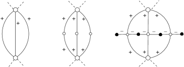
Furthermore, if we go around a small vertex in in any orientation, we encounter the edges from and not from alternately, see Figure 10 for an example. This can be observed by following the strand of a small -circle, since the crossings we encounter along this -circle are always negative, we either always arrive at the crossings on the overpass or always arrive at the crossings on the underpass (depending on the orientation we choose to travel), but the strands have to alternate between component 1 and component 2.
Consider an edge of that is on the boundary of a face in . If the lone edge connecting the small vertex of that is placed in and the medium vertex of that is on belongs to , we will say that is proper with respect to , otherwise we say that is improper with respect to . As we travers in any given orientation, we encounter proper and improper edges of with respect to alternately. We now construct a spanning tree of in the following way.
Step 1. Start with any face of , and choose any proper edge with respect to , and delete from the graph. This eliminates the face .
Step 2. Let be the face that shares with on its boundary, and choose a proper edge with respect to . Notice that it is necessary that . Delete from the graph and this eliminates the face .
Steps 3 to . We now continue this process. At each step, we choose a proper edge from the current face, which shares the proper edge chosen to be deleted from the previous edge on its boundary, to be deleted from the graph. Since there are faces, we can do this times and at the end we reach a spanning tree of . Notice that each corresponds to a unique negative edge not belonging to , see the right of Figure 10. Notice that on the right side of Figure 10, vertices marked by the same letter ( or ) are contracted to the same vertex due to the MP operations which are always performed in the direction from a medium vertex to a small vertex. The medium vertex pointed by the arrow is also contracted to the same vertex marked by .
Remark 5.4.
We observe first that MP operations can be performed on the crossings corresponding to the ’s, in the sequential order of , , …, , . The reason is that at each step brings with it a new medium vertex corresponding to a medium -circle that has not been affected by the previous MP operations, hence corresponds to a negative lone crossing and an MP operation can be performed on it using the direction from the medium -circle to the small -circle. Now consider the case when an edge is deleted (meaning its corresponding negative crossing is smoothed). Let be the edge that is paired with and let be the face of that contains , and use as the starting face to obtain the negative edges , . This time, as we perform the MP operations, the medium vertex that is connected to is shielded away from being swallowed by the combined vertices (due to the MP operations) since has been deleted. See the right side of Figure 10 for an illustration of this, where the edge marked by dashed line is deleted hence the vertex pointed by the arrow is not contracted by the MP operations. Therefore remains a lone edge after the MP operations discussed above are performed, and we can perform one more MP operation on the crossing corresponds to it. This means that if we smooth a negative crossing in , then we can perform MP operations on negative crossings, regardless whether some crossings in have been flipped or not, since the MP operations in the above discussion only used negative crossings not in .
We are now ready to prove Lemma 5.3.
Proof.
Choose any crossing in and apply skein relation (4.2) to it. We have . Notice that , . By Corollary 4.3 and Remark 5.4, we have
Thus the term will not make a contribution to the term. We now consider , which is obtained by flipping the crossing. We will choose another crossing from and repeat the above argument. Each time we can ignore the one obtained by smoothing the crossing. At the end, we arrive at a single term of the form where the diagram is obtained by flipping all crossings in . We observe that separates into two disjoint copies of (since component 1 now sits on top of component 2 at all crossings where they intersect), hence by Proposition 4.5. By Proposition 4.4, we have (keep in mind that ):
and
This proves that and ∎
5.4. The determination of and .
In this section we prove the following lemma.
Lemma 5.5.
If is a special alternating knot diagram with positive crossings, then and
Definition 5.6.
Let , where is the class of alternating knot diagrams defined in the proof of Lemma 5.2, such that the graph obtained from by removing the medium vertices is proper. Consider the link diagram corresponding to a Seifert graph obtained by placing a vertex (called a small vertex) in each face of , then adding an arbitrary number of edges between such a small vertex and the medium vertices on the boundary of the face that contains the small vertex. Each such edge corresponds to a negative crossing in the corresponding diagram. If a total of such edges are added, then the corresponding link diagram is denoted by .
Lemma 5.7.
Let be as defined in Definition 5.6. Let and be the numbers of large and medium vertices in , and be the number of faces in (which is the same as the number of small vertices in ), then and
Proof.
We use induction on . If , then is a disjoint union of and copies of trivial knots, hence the result follows from Proposition 4.5 and Lemma 5.2. Assume that this result is true for and consider the case . Choose any negative crossing in and apply (4.2) to it: with and (to which the induction hypothesis applies). There are two cases to consider.
Case 1: The negative crossing is not a lone crossing. In this case it is necessary that and simplifies (via a Reidemeister II move) to . Thus we have
with
On the other hand, we have
with
It follows that and .
Case 2. The negative crossing is a lone crossing, which corresponds to a (negative) lone edge connecting a small vertex and a medium vertex in . Again in this case the term yields the needed and , so it suffices to show that . Let be the face of containing and let be a spanning tree of that does not contain any edge on the boundary of . Since any edge in corresponds to two large vertices each connected to a common medium vertex by a (positive) lone edge, an MP operation can be performed using one of these lone crossings as shown in the left of Figure 11. The effect of this move is that and are swallowed by the newly created -circle. Since there are edges in , we can perform such operations. Furthermore, these operations do not affect the medium vertices on the boundary of , hence the flipped crossing remains a positive lone crossing, and one more MP operation can be performed. Thus we have . Notice that and . It follows from Corollary 4.3 that
∎
We are now ready to prove Lemma 5.5.
Proof.
If all maximal paths in are proper, then the statement of the lemma follows from Lemma 5.7 by substituting , and . Let us consider the case that contains maximal paths that are not proper. Remark 2.4, these maximal paths contain vertices that have degree 2 in . Furthermore, if there are multiple vertices with this property in a maximal path, they appear consecutively along the path, and the two end vertices of the path musth have degree more than 2 in . Let be the total number of degree 2 vertices in . Each such vertex is a large vertex of which has two lone edges connected to it. Of these two edges, we shall choose one that we encounter first by walking through the maximal path (it do not matter in which direction). Denote the set of these chosen edges by . We have . We now choose any crossing in and apply (4.1) to it: . We observe that smoothing a crossing in increases the number of MP operations in the diagram by one since the we have created a positive nugatory crossing which corresponds to an isolated medium -circle. That is, , , and . It follows that
Thus we shall ignore the term, and will continue the process with the term. That is, we start with diagram obtained by flipping the first crossing, and choose another crossing in , and apply (4.1) to it. Flipping the previously chosen crossings do not affect our ability to perform the MP operations based on any spanning tree of as described in Case 2 of the proof of Lemma 5.7, thus the same argument always applies to the diagram obtained by smoothing the crossing. At the end, we arrive at a term of the form , where is obtained by flipping every crossing in . Now observe that for each flipped crossing, a Reidemeister II move can be used to simplify the diagram: the result is that a large -circle and two medium -circles are combined into one medium -circle and the edges connecting to two medium -circles to small vertices are all connected to this newly created medium vertex. Thus, simplifies to a diagram as defined in Definition 5.6 with , and . By Lemma 5.7 we have
and
This shows that and . ∎
5.5. The determination of and .
We are now ready to derive explicit formulas for and as stated in the following lemma.
Lemma 5.8.
If , then and
with
On the other hand, if , then , and
with
Proof.
First consider the case . Use induction on . The case of has already been proved. Assume the lemma is true for some , consider the case . For , apply (4.1) to one of the positive crossings in the full positive twists: . Notice that deforms to the trivial knot, while simplifies to to which the induction hypothesis applies. Thus we have for any . On the other hand, if , then , with . If , then . We have and . Since , so . If , then we have hence with . This proves the case for .
For with , apply (4.2) to one of the negative crossings in the full negative twists: . Again deforms to the trivial knot, while for , simplifies to to which the induction hypothesis applies. Thus we have
for any . On the other hand, if , then
with
If , and , then
with . If , but , then , with since . Finally, if , then , with . ∎
Theorem 1.1 now follows from Lemma 5.8 easily. For example, if contains only positive crossings and , then we have
The case can be similarly obtained. If is a negative diagram, we can apply the above to the mirror image of first, then take the mirror image again. Passing to the mirror image does not change the number of crossings and the number of Seifert circles in the diagram, so the only change is the sign of .
6. Application to the ropelengths of knots
Let be an alternating link. We will call the largest braid index among all braid indices corresponding to different orientation assignments to the components of the maximum braid index of and denote it by . It has been shown recently that for some constant that is independent of (in fact ). Thus for a link , if is proportional to , then would be bounded below by a constant multiple of . For example, for the two component torus link , we have , hence . However, for a link with small maximum braid index, this result would be of little help to us. As a consequence of Theorem 1.1, we can prove the following theorem.
Theorem 6.1.
Let be a special alternating knot, then for some constant that is independent of .
Let us use a lattice realization of as a way to estimate . Let be a link and a realization of on the cubic lattice. The length of is denoted by and the minimum of over all lattice realization of is denoted by . The following result shows that bounds from below with serving as a bridge.
Proposition 6.2.
Proof.
Let be an arbitrary realization of in the cubic lattice and let be the length of it. The set is an embedding of the annulus into with and as its boundary curves. Denote by the oriented link formed by and such that they are assigned opposite orientations, then is equivalent to with where is the linking number of . By Theorem 1.1 we have . If we double the cubic lattice (so every edge is doubled and a new lattice point is inserted in the middle), then we obtain a realization of on the cubic lattice whose length is . By Proposition 6.2, we have . Since is arbitrary, this leads to . That is, , where is a constant which does not depend on . ∎
Remark 6.3.
Of course, the immediate question one may ask is, can Theorem 1.1 be generalized to alternating knots that are not special? We note that the proof of Theorem 1.1 relied on the nice structure of the Seifert circle decomposition of , hence that of . It is not clear to the author how to get around this, but the result in this paper is indeed very encouraging that the ropelength conjecture may hold in general for all alternating knots and links!
References
- [1] W. R. Bauer, F. H. C. Crick and J. H. White, Supercoiled DNA, Scientific American 243 (1) (Jul. 1980), 100–113.
- [2] G. Buck and J. Simon, Thickness and Crossing Number of Knots, Topology Appl. 91(3) (1999), 245–257.
- [3] G. Buck, Four-thirds Power Law for Knots and Links, Nature, 392 (1998), 238–239.
- [4] J. Cantarella, R. Kusner and J. Sullivan, Tight knot values deviate from linear relations, Nature, 392 (1998), 237–238.
- [5] Y. Diao, Braid Index Bounds Ropelength from Below, Journal of Knot Theory and its Ramifications, 29 (4) 2050019, 2020.
- [6] Y. Diao and C. Ernst, The Complexity of Lattice Knots, Topology and its Applications, 90 (1998), 1–9.
- [7] Y. Diao, C. Ernst and E. J. Jance Van Rensburg, Upper Bounds on Linking Number of Thick Links, J. Knot Theory Ramifications 11(2) (2002), 199–210.
- [8] Y. Diao, C. Ernst, A. Por and U. Ziegler, The Ropelengths of Knots Are Almost Linear in Terms of Their Crossing Numbers, Journal of Knot Theory and its Ramifications, 28 (14), 1950085, 2019. DOI: https://doi.org/10.1142/S0218216519500858.
- [9] Y. Diao, C. Ernst and M. Thistlethwaite, The Linear Growth in the Length of a Family of Thick Knots, J. Knot Theory Ramifications 12(5) (2003), 709–715.
- [10] Y. Diao, G. Hetyei and P. Liu The Braid Index Of Reduced Alternating Links, Math. Proc. Cambridge Philos. Soc., 168 (3) (2020), 415–434.
- [11] J. Franks and R. Williams Braids and The Jones Polynomial, Trans. Amer. Math. Soc., 303 (1987), 97–108.
- [12] P. Freyd, D. Yetter, J. Hoste, W. B. R. Lickorish, K. Millett and A. Ocneanu A New Polynomial Invariant of Knots and Links, Bulletin of the AMS, 12(2) (1985), 239–246.
- [13] P. Liu, Y. Diao and G. Hetyei The HOMFLY Polynomial of Links in Closed Braid Forms, Discrete Math., 342 (2019), 190–200.
- [14] H. Morton Seifert Circles and Knot Polynomials, Math. Proc. Cambridge Philos. Soc. 99 (1986), 107–109.
- [15] K. Murasugi On Alternating Knots, Osaka Math. J. 12 (1960), 277–303.
- [16] K. Murasugi and J. Przytycki An Index of a Graph with Applications to Knot Theory, Mem. Amer. Math. Soc. 106(508), 1993.
- [17] D. B. West, Introduction to Graph Theory, 2nd edition, Prentice Hall 2001.
- [18] J. White, Self-Linking and the Gauss Integral in Higher Dimensions, American Journal of Mathematics , Jul., 1969, 91 (3) (1969), 693–728.
- [19] S. Yamada The Minimal Number of Seifert Circles Equals The Braid Index of A Link, Invent. Math. 89 (1987), 347–356.