A Factor-Graph Approach for Optimization Problems
with Dynamics Constraints

Abstract

In this paper, we introduce dynamics factor graphs as a graphical framework to solve dynamics problems and kinodynamic motion planning problems with full consideration of whole-body dynamics and contacts. A factor graph representation of dynamics problems provides an insightful visualization of their mathematical structure and can be used in conjunction with sparse nonlinear optimizers to solve challenging, high-dimensional optimization problems in robotics. We can easily formulate kinodynamic motion planning as a trajectory optimization problem with factor graphs. We demonstrate the flexibility and descriptive power of dynamics factor graphs by applying them to control various dynamical systems, ranging from a simple cart pole to a 12-DoF quadrupedal robot.

I Introduction & Related Work

Rigid-body dynamics is a fundamental problem that is often involved in the study of robotics. Specifically, roboticists use inverse dynamics algorithms to compute motor torques in many control problems and forward dynamics algorithms in simulators. Researchers have proposed a variety of algorithms to solve the inverse dynamics problem, including RNEA [41, 19, 48]. Similarly, algorithms like the Composite-Rigid-Body Algorithm (CRBA) [60, 18], and the Articulated-Body Algorithm (ABA) [17] have been proposed to solve the forward dynamics problem. Rodriguez [52, 51] built a unified framework based on the concept of filtering and smoothing to solve both inverse and forward dynamics problems. Based on the work by Rodriguez et al. [53], Jain [30, 31, 32, 33] applied graph theory to dynamics problems, and analyzed various algorithms to solve dynamics problem in a unified formulation. Ascher et al. [1] unified the derivation of CRBA and ABA as two elimination methods used to solve forward dynamics. Various physics engines implement these algorithms, including RBDL [19], Bullet Physics [10], ODE [57], MuJoCo [59], DART [39], Pinocchio [8], etc. However, these dynamics algorithms are not intuitive to understand, and they usually act like black boxes in those physics engines. Hence, it is difficult to leverage these tools to solve various practical problems with dynamics involved, such as optimal control, kinodynamic motion planning, system modeling, state estimation, and simulation.

Developing a single mathematical representation that allows for optimization of controls for arbitrary dynamical systems is not trivial. Much prior work requires expert knowledge of a system’s dynamics to develop motion planning algorithms tailored to a particular system. In legged locomotion, various simplified dynamics models have been proposed to enable the control of legged robots. For instance, Kajita et al. [36] model a bipedal robot as a linear inverted pendulum, which enables control of the robot’s center of mass position along a plane. Blickhan et al. [6] further refine this dynamics model by adding a spring element, thereby enabling more sophisticated trotting and hopping gaits. Dai et al. [11] employs the centroidal dynamics model, which neglects the robot’s time-varying inertia matrix and uses Newton’s second law of translation and rotation to model the effect of contact forces on the robot’s linear and angular acceleration. Researchers studying the control of UAVs also utilize simplified dynamics models [61]. These simplified dynamics models are often exploited in trajectory optimization to optimize over motion plans [62, 63]. However, extending these trajectory optimization techniques to control other robotic systems requires significant effort and expert knowledge, as careful consideration of the robot’s dynamics is required to ensure that optimized trajectories are still valid for a new system. Posa et al.  [50] introduces a framework that allows for trajectory optimization of dynamical systems with contacts but only demonstrates its application to a single planar bipedal robot. Mordatch et al. [43] introduces Contact-Invariant Optimization, a behavior synthesis framework that leverages a simplified dynamics model to produce a wide variety of human behaviors for animated characters.

In this work, we introduce dynamics factor graphs (DFGs) as a framework for solving classical dynamics problems and advanced problems in control and motion planning. We leverage the descriptive power of DFGs to model a variety of systems, ranging from the nonlinear cart-pole to a 7-DoF Kuka Arm to a 12-DoF quadrupedal robot. We then incorporate DFGs into a trajectory optimization framework and use state-of-the-art sparse nonlinear optimizers to generate motion plans for various robots, all without requiring simplified dynamics models or expert knowledge of the robot’s dynamics a-priori. The main contributions are:

• A graphical representation of dynamics problems with factor graphs;

• Demonstration of solving a large variety of problems in robotics with factor graphs, including classical dynamics, dynamics with constraints and objectives, and kinodynamic motion planning;

• Demonstration of using a state-of-the-art sparse nonlinear optimizer based on GTSAM and a hinge loss formulation of inequality constraints to solve high-dimensional optimization problems in robotics.

II Review of Manipulator Dynamics

We briefly review the modern geometric view of robot dynamics and follow the exposition and notation from the recent text by Lynch and Park [42]. As convincingly argued in their introduction, this geometric view pioneered by Brockett [7] and Murray et al. [47] unlocks the powerful tools of modern differential geometry to reason about robot dynamics. It will also help below in describing the various dynamics algorithms in a concise graphical representation.

Closely following Section 8.3 in [42], applying this to the links of a serial manipulator and taking into account the constraints at the joints, we obtain four equations relating both link and joint quantities. In particular, the twist and acceleration $\mathcal{V}_{i}$ and $\mathcal{\dot{V}}_{i}$ for the $i$^th link are expressed in a body-fixed coordinate frame rigidly attached to the link. The wrench transmitted through joint $i$ is denoted as $\mathcal{F}_{i}$, and $\mathcal{G}_{i}$ is the link’s inertia matrix. Without loss of generality, below we assume all rotational joints, and we then have:

$$\mathcal{V}_{i}-[Ad_{T_{i,i-1}(\theta_{i})}]\mathcal{V}_{i-1}-\mathcal{A}_{i}\dot{\theta}_{i} =0$$ (1)

$$\mathcal{\dot{V}}_{i}-[Ad_{T_{i,i-1}(\theta_{i})}]\mathcal{\dot{V}}_{i-1}-\mathcal{A}_{i}\ddot{\theta}_{i}-[ad_{\mathcal{V}_{i}}]\mathcal{A}_{i}\dot{\theta}_{i} =0$$ (2)

$$Ad^{T}_{T_{i+1,i}(\theta_{i+1})}\mathcal{F}_{i+1}-\mathcal{F}_{i}+\mathcal{G}_{i}\dot{\mathcal{V}}_{i}-[ad_{\mathcal{V}_{i}}]^{T}\mathcal{G}_{i}\mathcal{V}_{i} =0$$ (3)

$$\mathcal{F}_{i}^{T}\mathcal{A}_{i}-\tau_{i} =0$$ (4)

where $\mathcal{A}_{i}$ is the screw axis for joint $i$ (expressed in link $i$), and $Ad_{T_{i,i-1}(\theta_{i})}$ is the adjoint transformation associated with the transform $T_{i,i-1}$ between the links (a function of $\theta_{i}$).

The four equations (1)-(4) express the dynamic constraints between link $i$ and link $i-1$ imposed by joint $i$: (1) describes the relationship between twist $\mathcal{V}_{i}$ and twist $\mathcal{V}_{i-1}$, where $\dot{\theta}_{i}$ is the angular velocity of joint $i$; (2) describes the constraint between acceleration $\mathcal{\dot{V}}_{i}$ and acceleration $\mathcal{\dot{V}}_{i+1}$, which involves components due to joint acceleration $\ddot{\theta}_{i}$ and the acceleration caused by rotation; (3) describes the balance between the wrench $\mathcal{F}_{i}$ through joint $i$ and the wrench $\mathcal{F}_{i+1}$ applied through joint $i+1$; (4) describes that the torque applied at joint i equals to the projection of wrench $\mathcal{F}_{i}$ on the screw axis $\mathcal{A}_{i}$ corresponding to joint $i$. Gravity is not considered above but can easily be accounted for using a ”trick” described by Lynch & Park [42] that adds an extra acceleration term to the base.

III A Factor Graph Approach

This paper proposes to represent optimal control problems involving dynamic constraints using a factor graph [37], a graphical model to describe the structure of sparse computational problems. A factor graph consists of factors and variables, where factors correspond to objectives, equality constraints, and inequality constraints involving the variables being optimized over. Variables are only connected to factors that they are involved in, and the resulting bipartite graph reveals the sparsity of the computation and enables the use of efficient optimization techniques. Factor graphs have been used in constraint satisfaction [55, 21, 12], AI [49, 56, 38, 22, 37], sparse linear algebra [23, 24, 29], information theory [58, 40], combinatorial optimization [4, 3, 5], and query theory [2, 25]. They have been successfully applied in other areas of robotics, such as SLAM [35, 34, 14, 20] and state estimation in legged robots [28, 64].

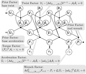
Figure 1: Dynamics factor graph for a RRR robot.

III-A Factor Graphs for Constrained Optimization

A constrained optimization problem may be written as

$$\min_{\boldsymbol{\chi}} f(\boldsymbol{\chi})$$ (5)

s.t. $$g_{i}(\boldsymbol{\chi})=0\,\text{ for }i=1,\dots,n$$

$$h_{j}(\boldsymbol{\chi})\leq 0\text{ for }j=1,\dots,m$$

where $g_{i}(\boldsymbol{x})$, $i=1,\dots,n$ and $h_{j}(\boldsymbol{x})$, $j=1,\dots,m$ are equality and inequality constraints, respectively and $f(\boldsymbol{x})$ is an objective function which we wish to optimize subject to the constraints. We convert the constrained problem into an unconstrained problem as follows:

$$\boldsymbol{\chi}^{*}= \min_{\boldsymbol{\chi}}\|r_{f}(\boldsymbol{\chi})\|^{2}_{\Sigma_{f}}+\sum_{i=1\dots\text{n}}\|r_{g,i}(\boldsymbol{\chi})\|^{2}_{\Sigma_{g,i}}$$ (6)

$$\qquad\qquad\qquad\,\,\,+\sum_{j=1\dots\text{m}}\|r_{h,j}(\boldsymbol{\chi})\|^{2}_{\Sigma_{\tilde{h},j}}$$

where $r_{f}(\boldsymbol{\chi})=\log{f(\boldsymbol{\chi})}$ is the log value of the objective function, $r_{g,i}(\boldsymbol{\chi})=\log{g_{i}(\boldsymbol{\chi})}$ are the log residual error functions associated with equality constraints, and $r_{h,j}(\boldsymbol{\chi})=\log{\tilde{h}_{j}(\boldsymbol{\chi})}=\log{\max(0,h_{j}(\boldsymbol{\chi}))}$ is the log of a hinge loss approximation of the residual error associated with the inequality constraints. The objective function $f(\boldsymbol{\chi})$, equality constraints $g_{i}(\boldsymbol{\chi})$, and inequality constraints $h_{j}(\boldsymbol{\chi})$ may all be represented as factors in a factor graph. Fig. 4 shows a schematic representation of a factor graph, where solid nodes correspond to objective functions or constraints.

III-B Dynamics Factor Graphs (DFGs)

We use a factor graph to represent the structure of the dynamics constraints (1)-(4) for a particular robot configuration. Fig. 1 illustrates this for a serial chain comprised of three revolute joints (RRR). Variables including twists $\mathcal{V}_{i}$, accelerations $\mathcal{\dot{V}}_{i}$, wrenches $\mathcal{F}_{i}$, joint angles $\theta_{i}$, joint velocities $\dot{\theta}_{i}$, joint accelerations $\ddot{\theta}_{i}$, and torques $\tau_{i}$ are constrained to satisfy the rigid-body dynamics equations (1)-(4). We can use the dynamics factor graph corresponding to all variables and constraints to model various dynamical systems, ranging from serial manipulators with fixed bases to legged robots with floating bases. We can also use them to solve classical dynamics problems (i.e., inverse and forward dynamics problems) and optimization problems in motion planning, as discussed in the sections below.

IV Solving Classical Dynamics Problems

This section demonstrates how to solve inverse and forward dynamics problems with DFGs and illustrate the classical dynamics algorithms within this framework.

IV-A Inverse Dynamics

(a) Simplified inverse DFG

(b) Eliminate all the $\tau$.

(c) Eliminate all the $\mathcal{F}$.

(d) Eliminate all the $\mathcal{\dot{V}}$.

Figure 2: Steps in elimination on the inverse DFG.

In inverse dynamics, we seek the joint torques $\tau_{i}$ to realize the desired joint accelerations $\ddot{\theta}_{i}$. We can construct a simplified, less cluttered, inverse dynamics graph by replacing all known variables with constants in the factors to which they are connected. Fig. 2(a) shows the DFG for a RRR robot, corresponding to the nine linear constraints of the 3R inverse dynamics problem. Solving the inverse dynamics problem is equivalent to solving this factor graph, and it can be done by back-substitution after performing elimination on the graph.

We illustrate the elimination process in the 3R case for a particular ordering in Fig. 2. The elimination is performed in the order $\tau_{3}\ \tau_{2}\ \tau_{1}$, $\mathcal{F}_{1}\ \mathcal{F}_{1}\ \mathcal{F}_{3}$, $\mathcal{\dot{V}}_{3}\ \mathcal{\dot{V}}_{3}\ \mathcal{\dot{V}}_{1}$. Fig. 2(b) shows the result of first eliminating the torques $\tau_{i}$, where the arrows show that the torques $\tau_{i}$ only depend on the corresponding wrenches $\mathcal{F}_{i}$. We then eliminate $\mathcal{F}_{1}$, which results in a dependence of $\mathcal{F}_{1}$ on $\mathcal{\dot{V}}_{1}$ and $\mathcal{F}_{2}$. After eliminating all the wrenches, we get the result as shown in Fig. 2(c). Finally, we eliminate the all the twist accelerations $\mathcal{\dot{V}}_{3}\ \mathcal{\dot{V}}_{3}\ \mathcal{\dot{V}}_{1}$, in that order. After completing all these elimination steps, the inverse dynamics factor graph in Fig. 2(a) is thereby converted to the directed acyclic graph (DAG) as shown in Fig. 2(d).

After elimination, back-substitution in reverse elimination order solves for the values of all intermediate quantities and the desired torques. For the example ordering in 2, back-substitution first computes the 6-dimensional accelerations $\mathcal{\dot{V}}_{i}$, then the link wrenches $\mathcal{F}_{i}$, and finally the scalar torques. This exactly matches the forward-backward path used by the recursive Newton-Euler algorithm (RNEA) [41].

IV-B Forward Dynamics

(a)

(b)

(c)

Figure 3: (a) Simplified forward DFG; (b) CRBA ordering DAG; (c) ABA ordering DAG.

In traditional expositions, the forward dynamics problem cannot be solved as neatly as the relatively easy inverse dynamics problem. In the forward case, we seek the joint accelerations $\ddot{\theta}$ when given $\theta$, $\dot{\theta}$, and $\tau$. Similar to the inverse dynamics factor graph, we can simplify the forward dynamics factor graph, as shown in Fig. 3(a).

In the same spirit as our work, Ascher et al. [1] shows that two of the most widely used forward dynamics algorithms, CRBA [18] and ABA [17], can be explained as two different elimination methods to solve the same linear system.

In our framework, CRBA and ABA can also be visualized as two different DAGs resulting from solving the forward dynamics factor graph with two different elimination orders shown in Fig. 3(b) and Fig. 3(c). CRBA first eliminates all the wrenches $\mathcal{F}_{i}$, then eliminates all the accelerations $\mathcal{\dot{V}}_{i}$, and eliminates all the angular accelerations $\ddot{\theta}_{i}$ last. In contrast, in ABA we alternate between eliminating the wrenches $\mathcal{F}_{i}$, accelerations $\mathcal{\dot{V}}_{i}$ and angular accelerations $\ddot{\theta}_{i}$ for $i\in n\dots 1$. We can view the resulting DAGs as graphical representations of CRBA and ABA, and for a given robot configuration, we can write a custom back-substitution program in reverse elimination order.

V Solving Constrained Dynamics Problems

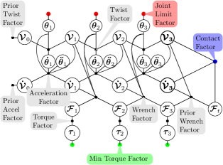
Figure 4: Constrained dynamics factor graph for a RRR robot.

This section briefly explains how to solve dynamics problems with joint limit constraints, contacts, task-dependent objectives, and redundancy resolution. The complexity of practical problems in robotics far surpasses that of the previous section’s classical problems. For instance, the system has to stay within its joint limits at any time instance to avoid damage. Redundancy issues often occur when the system is not fully constrained, for instance, solving inverse dynamics for a manipulator with kinematic loops or planning motion for tasks in which we constrain the external wrench acting on the end-effector in only one direction. Also, when there is contact involved in the motion, the dynamics problem becomes even more complicated. In motion planning or optimal control literature, joint limits and contacts are usually represented as constraints in the optimization problem, and the redundancy issue can be resolved by optimizing for a minimum torque objective.

Here, we propose to solve all these problems with DFGs by incorporating them as factors in the graph, as shown in Fig. 4. We then solve the constrained optimization dynamics problem with GTSAM [13, 14].

V-A Joint Limit Factors

Joint limits are formulated as the following inequality constraint for each joint angle $q_{i}$, $h_{\text{lim}}(q_{i})-\theta_{\text{lim, i}}\leq 0$, where $\theta_{\text{lim, i}}$ is the limit for the i^th joint. We incorporate this inequality in a hinge loss function:

$$\tilde{h}_{\text{lim}}(q_{i})=\left\{\begin{array}[]{ll}\alpha(\theta_{\text{lim, lower}}-q_{\text{i}}+\varepsilon)&{\text{if }\ q_{\text{i}}-\theta_{\text{lim, i}}\leq\varepsilon}\\ \alpha(q_{\text{i}}-\theta_{\text{lim, upper}}+\varepsilon)&{\text{if }\ \theta_{\text{lim, upper}}-q_{\text{i}}\leq\varepsilon}\\ 0&{\text{otherwise}}\end{array}\right.$$ (7)

where $\theta_{\text{lim, lower}}$ is the lower limit, $\theta_{\text{lim, upper}}$ is the upper limit, $\varepsilon$ is a constant threshold to prevent exceeding the limit, and $\alpha$ is a constant ratio which determines how fast the error grows as the value approaches the limit. If the value is within the threshold, then the cost is 0. Hence, the limit violations are prevented during the optimization. This technique is characteristic of interior point method [15].

V-B Minimum Torque Factor

Minimum torque objective is formulated as an equality constraint, and cost function can be expressed as $g_{\tau}(\tau_{i})=\tau_{i}$, where $\tau_{i}$ is the torque at joint $i$. The cost grows as the torque increases, and we can expect that the optimizer solves for a solution with minimum torque values.

V-C Contact Factor (Friction Cone)

A desirable property of legged locomotion controllers is to provide robustness against slipping motions. This property benefits the robot’s stability and improves locomotion efficiency. A common approach to avoid slipping motions is to constrain the contact forces at the end-effectors to lie within a friction cone [62, 26]. This inequality constraint prevents the lateral forces from dominating the resistive Coulomb friction forces, thereby preventing slipping. Consider the external wrench at the robot’s i^th end-effector $\mathcal{F}_{i}^{e}=[m_{i}^{e};f_{i}^{e}]\in\chi$. The contact factor enforces the following inequality constraint:

$$\|f_{i}^{e}-(f_{i}^{e}\cdot n_{i})n_{i}\|_{2}\leq\mu_{i}(f_{i}^{e}\cdot n_{i})$$

$\mu_{i}$ is the static friction coefficient at the i^th contact, and $b_{i}$ is the vector normal to the surface. This inequality constraint is enforced using a hinge loss function and incorporated as a factor connected to each end-effector in the DFG.

VI Motion Planning with Dynamics Factor Graph (DFGP)

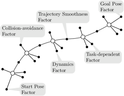
Figure 5: kinodynamic motion planning factor graph, where solid nodes indicate factors and hollow nodes correspond to the decision variables.

After solving the constrained dynamics problem, motion planning with the whole-body dynamics constraints becomes straightforward. A simple intuition is that we can view the constrained dynamics problem as a single time instance of the motion planning problem and incorporate the constrained dynamics factor graphs into a trajectory optimization problem in the style of GPMP2 [45], as shown in Fig. 5. To accomplish a real motion planning task, we need to add a few more factors to the graph. For instance, we use initial and goal pose factors to satisfy the demand of moving the end-effector from the initial pose to a goal pose, trajectory smoothness factors are applied to encourage smooth trajectories, and we add collision avoidance factors to ensure collision-free motion. Other task-dependent factors can be easily incorporated into a DFG as well. Due to the page limit, we only briefly describe the trajectory smoothness factor, which is only slightly different from the one outlined in GPMP2. For details on start and goal factors and collision avoidance factors, one can refer to GPMP2 [45].

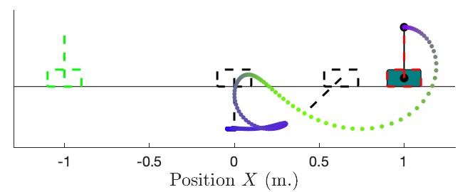
(a)

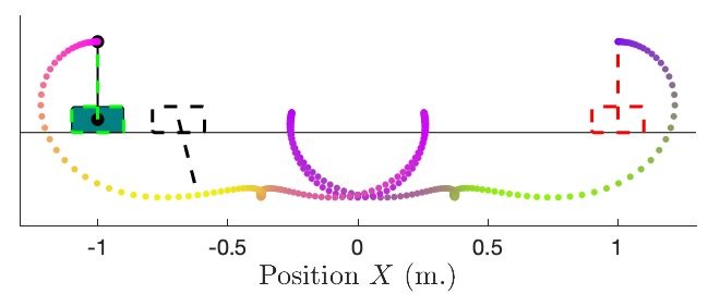
(b)

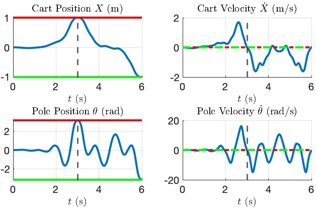
(c)

Figure 6: The DFGP was used optimize a trajectory for the cart-pole system that achieves two configurations in quick succession. (a) and (b) show the trajectory generated to reach the 1st and 2^nd configuration, respectively. (c) demonstrates that the optimized trajectory satisfies the constraints imposed for the 1st (t = 3s) and 2nd configuration (t = 6s), shown as red and green bars, respectively. (See supplemental videos)

VI-A Trajectory Smoothness Factor

Here we describe a method which we use to optimize smooth trajectories using DFGs and additional trajectory factors. We use a method similar to the one discussed in GPMP2, but with the assumption of a continuous-time configuration space trajectory with a constant acceleration instead of constant velocity, and add a Gaussian process (GP) smoothness prior with cost function, $g_{m}(x_{i-1},x_{i})=x_{i}-\Phi(t_{i},t_{i-1})x_{i-1}$ and covariance matrix

$$\Sigma=\begin{bmatrix}\frac{1}{2}\Delta t_{i}^{5}\mathbf{Q}_{C}&\frac{1}{8}\Delta t_{i}^{4}\mathbf{Q}_{C}&\frac{1}{6}\Delta t_{i}^{3}\mathbf{Q}_{C}\\ \frac{1}{8}\Delta t_{i}^{4}\mathbf{Q}_{C}&\frac{1}{3}\Delta t_{i}^{3}\mathbf{Q}_{C}&\frac{1}{2}\Delta t_{i}^{2}\mathbf{Q}_{C}\\ \frac{1}{6}\Delta t_{i}^{3}\mathbf{Q}_{C}&\frac{1}{2}\Delta t_{i}^{2}\mathbf{Q}_{C}&\Delta t_{i}\mathbf{Q}_{C}\end{bmatrix}$$ (8)

where $\mathbf{Q}_{C}$ is the power-spectral density matrix associated with the GP. We also define the state transition matrix

$$\Phi(t_{i},t_{i-1})=\begin{bmatrix}1&\Delta t_{i}&\frac{1}{2}(\Delta t_{i})^{2}\\ 0&1&\Delta t_{i}\\ 0&0&1\end{bmatrix}$$ (9)

associated with a constant acceleration assumption between times $t_{i-1}$ and $t_{i}$, and $\Delta t_{i}=t_{i}-t_{i-1}.$

VI-B Kinodynamic Motion Planning Factor Graph

A kinodynamic motion planning factor graph, as shown in Fig. 5, is designed to solve the kinodynamic motion planning problem[16], in which both constraints and objectives are represented as factors. In particular, we use constrained DFGs for each time instance, and connect them with trajectory smoothness factors (Section VI-A) to encourage smooth trajectories. In addition, the initial pose constraint, goal pose constraint, and obstacle avoidance objective are included to fulfill the task while avoiding collisions.

VII Experiments

We implemented DFGP using the GTSAM Factor Graph optimization library [13, 14], and ran simulations in V-REP [54] and PyBullet [10] for visualization.

VII-A Cart Pole

The cart-pole system is composed of an unactuated simple pendulum attached to a wheeled cart. A common task in optimal control is to balance the pendulum around its unstable equilibrium, using only horizontal forces on the cart. In this experiment, we tackle a more sophisticated control problem that involves driving the cart-pole system to multiple goal configurations in quick succession. We apply our DFGP algorithm to optimize for a single trajectory that enables the cart-pole system to achieve two goal configurations at prescribed times. We apply a zero-torque constraint on the unactuated pendulum. We also apply the trajectory smoothness factors discussed in section VI-A and the minimum torque objective discussed in section V-B. Two goal configurations are imposed as objectives in the trajectory factor graph:

$$f_{\mathrm{goal,}t=\eta s}(\chi)=\|\theta_{t=\eta s}-\theta_{t=\eta s}^{*}\|+\|p_{t=\eta s}-p_{t=\eta s}^{*}\|$$ (10)

Where $p$ and $\theta$ are the cart-pole’s horizontal position and pole angle, respectively. The first configuration requires that the cart-pole come to rest at $[p_{\mathrm{t=3s}}^{*},\theta_{\mathrm{t=3s}}^{*}]=[1m,\pi\mathrm{rad}]$. The second configuration requires that the cart-pole come to rest at $[p_{\mathrm{t=6s}}^{*},\theta_{\mathrm{t=6s}}^{*}]=[-1m,-\pi\mathrm{rad}]$. Figures 6(a) and 6(b) visualize the cart-pole’s execution of the optimized trajectory. Fig. 6(c) demonstrates that the DFGP trajectory satisfies both the position and velocity objectives for both configurations.

VII-B Kuka Arm

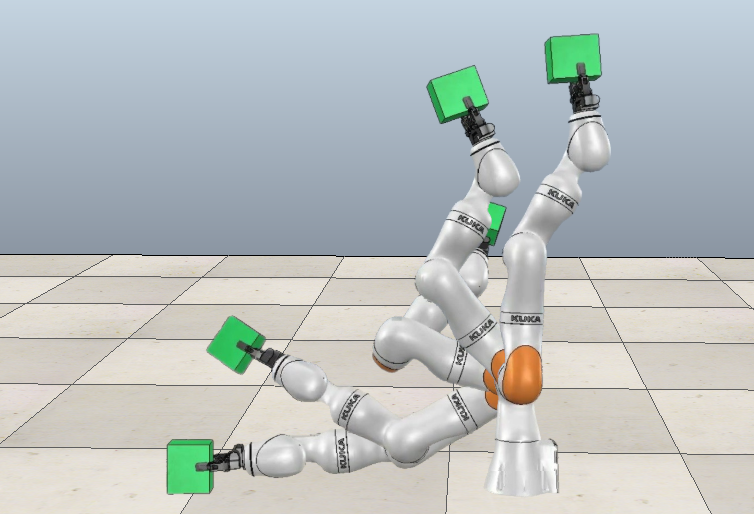
(a)

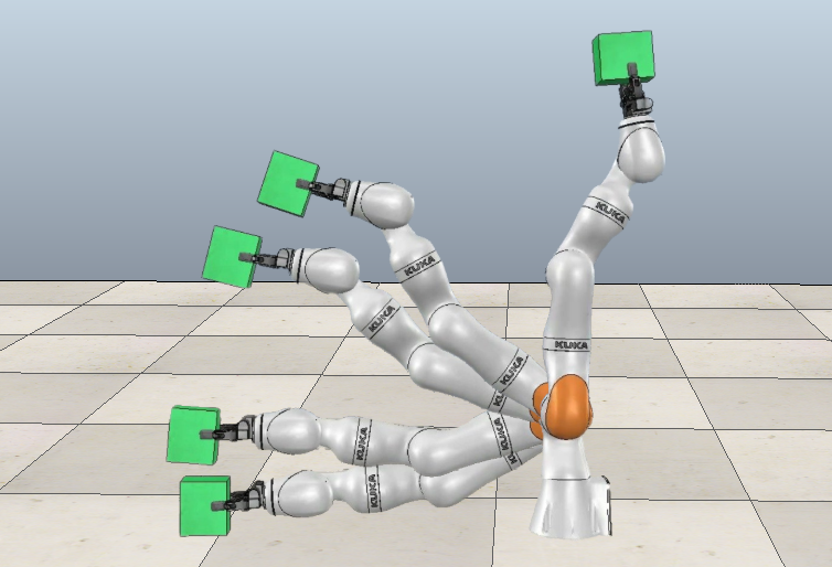
(b)

Figure 7: (a) DFGP solution with minimum torque constraint; (b) DFGP solution without minimum torque constraint (See supplemental videos). More details are described in Section VII-B

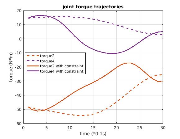
Figure 8: Torque trajectories of Kuka arm experiment. More details are described in Section VII-B.

The KUKA LBR iiwa [9] is a lightweight industry robot with seven actuated revolute joints. The task performed in this experiment is to move a block from the floor to its upright position. Fig. 7(a) and Fig. 7(b) show solutions obtained by DFGP with and without the minimum torque objective, respectively. In Fig. 7(a), we observe that the Kuka arm first moves towards the center to reduce the moment arm, and then pushes upwards so that it can bring the block to the goal location with less torque applied when compared to the solution shown in Fig. 7(b).

We plot the torque trajectories corresponding to the 2^nd and 4^th joints of the Kuka arm in Fig. 8 (the two joints with the highest energy consumption). The solid lines and dashed lines represent the torque trajectories optimized using DFGP with and without the minimum torque constraint. We observe that DFGP produces a more energy-efficient motion plan when we add the minimum torque factor to the graph.

VII-C Quadruped

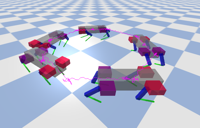
(a)

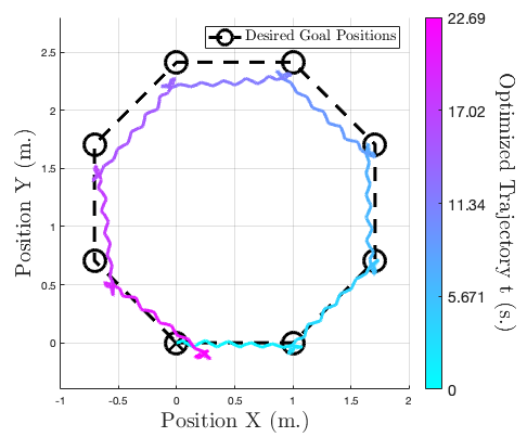
(b)

Figure 9: Trajectory for a quadrupedal robot optimized using DFGP and executed in an open loop manner. The dashed line represents the desired CoM trajectory for the given contact schedule. The gradated line represents the actual CoM trajectory when the optimized trajectory is executed in an open-loop fashion. Our method exhibits low error due to its consideration of the full dynamics and kinematics.(See supplemental videos)

Motion planning for legged robots is a challenging, high-dimensional optimization problem. The difficulty arises from the contacts, as the addition and removal of contacts with the environment leads to time-varying dynamics constraints. Here we use DFGP to optimize an open-loop trajectory for a 12-DoF quadrupedal robot. We task DFGP with optimizing a trajectory that guides the robot through six navigation waypoints. The waypoints are placed on the vertices of a hexagon with a side length of $1.6m$ (See Fig. 9(b)).

We define a kinodynamic motion planning factor graph and add additional inequality constraints and objectives. Specifically, we incorporate the contact factor defined in Section V-C to ensure that the legged robot does not slip. We also apply a minimum torque factor to encourage efficiency and joint limit factors to prevent violation of the robot’s joint limits. In this problem, we add a prior over the robot’s contact sequence and use GTSAM to optimize for a valid trajectory.

As shown in Fig. 9, the trajectory generated by our system is highly accurate, leading to little model error even when executed in an open-loop fashion. The high tracking accuracy can be explained by our DFG formulation, which models the whole-body dynamics and does not rely on simplified dynamics models.

VIII Discussion

We introduce dynamics factor graphs (DFGs) as a useful framework for solving various problems in robotics. Our approach treats rigid-body dynamics constraints as factors in a factor graph and optimizes the variables to achieve an objective subjects to dynamics constraints. We also demonstrated how to extend DFGs to support inequality constraints and objective functions. Finally, we introduced DFGP, a motion-planning algorithm that leverages DFGs and trajectory smoothness factors to optimize motion plans for arbitrary robotic systems.

In Section IV, we demonstrated the application of DFGs to classical dynamics problems, such as forward and inverse dynamics. We saw how our framework intuitively explains various well-known classical dynamics algorithms as DAGs resulting from the solving of the DFG with different elimination orders. We also showed how DFGP can be used to solve practical problems in control and trajectory optimization. We were able to optimize trajectories for three very different robotics systems using a single tool.

In future work, we hope to perform incremental kinodynamic motion planning in the style of GPMP2 [46] and STEAP [44], which successfully applied incremental inference in factor graphs [34, 14] to kinematic motion planning problems. Also, it would be exciting to use the factor-graph-based representation of dynamics to perform state estimation for dynamically balanced robots, in the spirit of Hartley et al. [28, 27] and Wisth et al. [64].

References

- [1] U. M. Ascher, P. K. Dinesh, and B. P. Cloutier. Forward dynamics, elimination methods, and formulation stiffness in robot simulation. The International Journal of Robotics Research, 16(6):749–758, 1997.
- [2] C. Beeri, R. Fagin, D. Maier, A. Mendelzon, J. Ullman, and M. Yannakakis. Properties of acyclic database schemes. In ACM Symp. on Theory of Computing (STOC), pages 355–362, New York, NY, USA, 1981. ACM Press.
- [3] U. Bertele and F. Brioschi. On the theory of the elimination process. J. Math. Anal. Appl., (1):48–57, July.
- [4] U. Bertele and F. Brioschi. Nonserial Dynamic Programming. Academic Press, 1972.
- [5] U. Bertele and F. Brioschi. On nonserial dynamic programming. J. Combinatorial Theory, 14:137–148, 1973.
- [6] R. Blickhan. The spring-mass model for running and hopping. J Biomech, 22(11-12):1217–1227, 1989.
- [7] W. Roger Brockett. Robotic manipulators and the product of exponentials formula. In Mathematical theory of networks and systems, pages 120–129. Springer, 1984.
- [8] J. Carpentier, G. Saurel, G. Buondonno, J. Mirabel, F. Lamiraux, O. Stasse, and N. Mansard. The Pinocchio C++ library – A fast and flexible implementation of rigid body dynamics algorithms and their analytical derivatives. In International Symposium on System Integration (SII), 2019.
- [9] KUKA Robotics Corporation. KUKA LBR iiwa, 2019.
- [10] Erwin Coumans and Yunfei Bai. Pybullet, a python module for physics simulation for games, robotics and machine learning. http://pybullet.org, 2016–2019.
- [11] H. Dai, A. Valenzuela, and R. Tedrake. Whole-body motion planning with centroidal dynamics and full kinematics. In 2014 IEEE-RAS International Conference on Humanoid Robots, pages 295–302, 2014.
- [12] R. Dechter and J. Pearl. Network-based heuristics for constraint-satisfaction problems. Artificial Intelligence, 34(1):1–38, December 1987.
- [13] F. Dellaert. Factor graphs and gtsam: A hands-on introduction. Technical report, Georgia Institute of Technology, 2012.
- [14] F. Dellaert and M. Kaess. Factor graphs for robot perception. Foundations and Trends in Robotics, 6(1-2):1–139, 2017.
- [15] I. Dikin. Iterative solution of problems of linear and quadratic programming. 174(4):747–748, 1967.
- [16] Bruce Donald, Patrick Xavier, John Canny, John Canny, John Reif, and John Reif. Kinodynamic motion planning. Journal of the ACM (JACM), 40(5):1048–1066, 1993.
- [17] R. Featherstone. The calculation of robot dynamics using articulated-body inertias. The International Journal of Robotics Research, 2(1):13–30, 1983.
- [18] R. Featherstone and D. E. Orin. Robot dynamics: equations and algorithms. In Proceedings 2000 ICRA. Millennium Conference. IEEE International Conference on Robotics and Automation. Symposia Proceedings (Cat. No. 00CH37065), volume 1, pages 826–834. IEEE, 2000.
- [19] M. L. Felis. RBDL: An efficient rigid-body dynamics library using recursive algorithms. Autonomous Robots, 41(2):495–511, 2017.
- [20] C. Forster, L. Carlone, F. Dellaert, and D. Scaramuzza. On-manifold preintegration for real-time visual-inertial odometry. IEEE Trans. Robotics, 2017.
- [21] Eugene C. Freuder. A sufficient condition for backtrack-free search. J. ACM, 29(1):24–32, 1982.
- [22] B.J. Frey, F.R. Kschischang, H.-A. Loeliger, and N. Wiberg. Factor graphs and algorithms. In Proc. 35th Allerton Conf. Communications, Control, and Computing, pages 666–680, September 1997.
- [23] A. George, J. Liu, and Ng E. Row-ordering schemes for sparse Givens transformations. I. Bipartite graph model. Linear Algebra Appl, 61:55–81, 1984.
- [24] J.R. Gilbert and E.G. Ng. Predicting structure in nonsymmetric sparse matrix factorizations. In J.A. George, J.R. Gilbert, and J.W-H. Liu, editors, Graph Theory and Sparse Matrix Computations, volume 56 of IMA Volumes in Mathematics and its Applications. Springer-Verlag, New York, 1993.
- [25] N. Goodman and O. Shmueli. Tree queries: a simple class of relational queries. ACM Trans. Database Syst., 7(4):653–677, 1982.
- [26] Ruben Grandia, Farbod Farshidian, René Ranftl, and Marco Hutter. Feedback mpc for torque-controlled legged robots, 2019.
- [27] R. Hartley, M. G. Jadidi, L. Gan, J. Huang, J. W. Grizzle, and R. M. Eustice. Hybrid contact preintegration for visual-inertial-contact state estimation using factor graphs. In 2018 IEEE/RSJ International Conference on Intelligent Robots and Systems (IROS), pages 3783–3790, Oct 2018.
- [28] R. Hartley, J. Mangelson, L. Gan, M. Ghaffari Jadidi, J. M. Walls, R. M. Eustice, and J. W. Grizzle. Legged robot state-estimation through combined forward kinematic and preintegrated contact factors. In 2018 IEEE International Conference on Robotics and Automation (ICRA), pages 4422–4429, May 2018.
- [29] P. Heggernes and P. Matstoms. Finding good column orderings for sparse QR factorization. In Second SIAM Conference on Sparse Matrices, 1996.
- [30] A. Jain. Unified formulation of dynamics for serial rigid multibody systems. Journal of Guidance, Control, and Dynamics, 14(3):531–542, 1991.
- [31] Abhinandan Jain. Graph theoretic foundations of multibody dynamics part i: analysis and algorithms. Multibody system dynamics, 26(3):307, 2011.
- [32] Abhinandan Jain. Graph theoretic foundations of multibody dynamics part ii: analysis and algorithms. Multibody system dynamics, 26(3):335, 2011.
- [33] Abhinandan Jain. Multibody graph transformations and analysis: part i: tree topology systems. Nonlinear dynamics, 67(4), 2012.
- [34] M. Kaess, H. Johannsson, R. Roberts, V. Ila, J. Leonard, and F. Dellaert. iSAM2: Incremental smoothing and mapping using the Bayes tree. Intl. J. of Robotics Research, 31:217–236, Feb 2012.
- [35] M. Kaess, A. Ranganathan, and F. Dellaert. iSAM: Incremental smoothing and mapping. IEEE Trans. Robotics, 24(6):1365–1378, Dec 2008.
- [36] Shuuji Kajita, Fumio Kanehiro, Kenji Kaneko, Kazuhito Yokoi, and Hirohisa Hirukawa. The 3d linear inverted pendulum model: A simple modeling for a biped walking pattern generation. volume 1, pages 239 – 246 vol.1, 02 2001.
- [37] F.R. Kschischang, B.J. Frey, and H-A. Loeliger. Factor graphs and the sum-product algorithm. IEEE Trans. Inform. Theory, 47(2), February 2001.
- [38] S. L. Lauritzen and D. J. Spiegelhalter. Local computations with probabilities on graphical structures and their application to expert systems. Journal of the Royal Statistical Society. Series B (Methodological), 50(2):157–224, 1988.
- [39] Jeongseok Lee, Michael X Grey, Sehoon Ha, Tobias Kunz, Sumit Jain, Yuting Ye, Siddhartha S Srinivasa, Mike Stilman, and C Karen Liu. Dart: Dynamic animation and robotics toolkit. Journal of Open Source Software, 3(22):500, 2018.
- [40] H.-A. Loeliger. An introduction to factor graphs. IEEE Signal Processing Magazine, pages 28–41, January 2004.
- [41] J. Y. S. Luh, M. W. Walker, and R. P. Paul. On-line computational scheme for mechanical manipulators. Journal of Dynamic Systems, Measurement, and Control, 102(2):69–76, 1980.
- [42] K. M Lynch and F. C Park. Modern Robotics. Cambridge University Press, 2017.
- [43] Igor Mordatch, Emanuel Todorov, and Zoran Popović. Discovery of complex behaviors through contact-invariant optimization. ACM Trans. Graph., 31(4), July 2012.
- [44] M. Mukadam, J. Dong, F. Dellaert, and B. Boots. Steap: simultaneous trajectory estimation and planning. Autonomous Robots, pages 1–20, 2018.
- [45] M. Mukadam, J. Dong, X. Yan, F. Dellaert, and B. Boots. Continuous-time gaussian process motion planning via probabilistic inference. The International Journal of Robotics Research, 37(11):1319–1340, 2018.
- [46] M. Mukadam, J. Dong, X. Yan, F. Dellaert, and B. Boots. Continuous-time gaussian process motion planning via probabilistic inference. Intl. J. of Robotics Research, 37(11):1319–1340, 2018.
- [47] R.M. Murray, Z. Li, and S. Sastry. A Mathematical Introduction to Robotic Manipulation. CRC Press, 1994.
- [48] D. E. Orin, R. McGhee, M. Vukobratovi, and G. Hartoch. Kinematic and kinetic analysis of open-chain linkages utilizing newton-euler methods. Mathematical Biosciences, 43(1-2):107–130, 1979.
- [49] J. Pearl. Probabilistic Reasoning in Intelligent Systems: Networks of Plausible Inference. Morgan Kaufmann, 1988.
- [50] Michael Posa and Russ Tedrake. Direct trajectory optimization of rigid body dynamical systems through contact. In Emilio Frazzoli, Tomas Lozano-Perez, Nicholas Roy, and Daniela Rus, editors, Algorithmic Foundations of Robotics X, pages 527–542, Berlin, Heidelberg, 2013. Springer Berlin Heidelberg.
- [51] G. Rodriguez. Recursive forward dynamics for two robot arms in a closed chain based on kalman filtering and bryson-frazier smoothing. In Proceedings of the International Symposium on Robot Manipulators on Recent trends in robotics: modeling, control and education, pages 85–93. Elsevier North-Holland, Inc., 1986.
- [52] G. Rodriguez. Kalman filtering, smoothing, and recursive robot arm forward and inverse dynamics. IEEE Journal on Robotics and Automation, 3(6):624–639, 1987.
- [53] G. Rodriguez, A. Jain, and K. Kreutz-Delgado. A spatial operator algebra for manipulator modeling and control. The International Journal of Robotics Research, 10(4):371–381, 1991.
- [54] E. Rohmer, S. P. N. Singh, and M. Freese. Coppeliasim (formerly v-rep): a versatile and scalable robot simulation framework. In Proc. of The International Conference on Intelligent Robots and Systems (IROS), 2013. www.coppeliarobotics.com.
- [55] R. Seidel. A new method for solving constraint satisfaction problems. In Intl. Joint Conf. on AI (IJCAI), pages 338–342, 1981.
- [56] P. P. Shenoy and G. Shafer. Propagating belief functions using local computations,. IEEE Expert, 1(3):43–52, Fall 1986.
- [57] Russell Smith et al. Open dynamics engine. 2005.
- [58] R. Tanner. A recursive approach to low complexity codes. IEEE Trans. Inform. Theory, 27(5):533–547, Spetember 1981.
- [59] Emanuel Todorov, Tom Erez, and Yuval Tassa. Mujoco: A physics engine for model-based control. In 2012 IEEE/RSJ International Conference on Intelligent Robots and Systems, pages 5026–5033. IEEE, 2012.
- [60] M. W. Walker and D. E. Orin. Efficient dynamic computer simulation of robotic mechanisms. Journal of Dynamic Systems, Measurement, and Control, 104(3):205–211, 1982.
- [61] P. Wang, Z. Man, Z. Cao, J. Zheng, and Y. Zhao. Dynamics modelling and linear control of quadcopter. In 2016 International Conference on Advanced Mechatronic Systems (ICAMechS), pages 498–503, 2016.
- [62] A. W Winkler, C D. Bellicoso, M. Hutter, and J. Buchli. Gait and trajectory optimization for legged systems through phase-based end-effector parameterization. IEEE Robotics and Automation Letters, 3(3):1560–1567, 2018.
- [63] Alexander W Winkler, Farbod Farshidian, Diego Pardo, Michael Neunert, and Jonas Buchli. Fast trajectory optimization for legged robots using vertex-based zmp constraints, 2017.
- [64] D. Wisth, M. Camurri, and M. Fallon. Robust legged robot state estimation using factor graph optimization. IEEE Robotics and Automation Letters, 4(4):4507–4514, Oct 2019.